Environment tensor as order parameter for
symmetry breaking and (symmetry-protected) topological orders

Abstract

Spontaneous symmetry breaking is well understood through the classical “Mexican Hat” picture, which describe many quantum phases of matter. Recently, several new classes of quantum phases of matter, such as topological orders and symmetry protected topological (SPT) orders, were discovered. In an attempt to address the transitions between all those phases of quantum matter under the same framework, we introduced an analogous yet very simple picture for phase transitions in the context of tensor-networks. Using a very simple iteration process, we found that both symmetry breaking and some topological phase transitions (for topological orders described by gauge theory and 1D SPT orders) could be marked by a sudden change in the symmetry structure of the so-called “environment matrix”. In this process, the environment matrix serves as an “order parameter” that captures patterns of entanglement in topological phases. The symmetry change in the environment matrix is very much like the symmetry breaking of conventional order parameters. We applied this method to both the transverse Ising model ($1D$ and $2D$ honeycomb), spin-1 model ($1D$), and the Toric Code model in a magnetic field ($2D$ honeycomb), and explored the corresponding symmetry structure changes in their environment matrices in details. With just a few variational parameters and a few minutes’ run time on a laptop, we could get the corresponding phase transition points within a few percent error compared with the Quantum Monte Carlo results.

I Introduction

In recent years, with the discoveries of quantum Hall statesvon Klitzing et al. (1980); Tsui et al. (1982) and topological insulators,Kane and Mele (2005); Bernevig and Zhang (2006); Moore and Balents (2007); Fu et al. (2007); Kitaev (2009); Ryu et al. (2009) the field of condensed matter physics is focusing more and more on topological phases of matter. Lots of progress has been made in the classification of topological orderWen (1989); Wen and Niu (1990); Wen (1990); Keski-Vakkuri and Wen (1993) in interacting bosonic/fermionic systems through tensor network representation of many-body wave function and the associated fixed-point tensors under wave function renormalization,Levin and Wen (2005); Chen et al. (2010a); Liu et al. ; Gu et al. which lead to tensor category theory of topological order.Levin and Wen (2005); Chen et al. (2010a); Kong and Wen (2014); Barkeshli et al. (2014) In the presence of symmetry, tensor network and group cohomologyChen et al. (2012); Kapustin (2014); Wen (2014a) also lead to a classification of symmetry protected topological (SPT) order.Gu and Wen (2009)

However, an important question is how to determine the topological order or SPT order carried by a generic wave function or a generic tensor network wave function.Wen (1990); Keski-Vakkuri and Wen (1993); Wen (2012); Zhang et al. (2012); Cincio and Vidal (2013); Zaletel et al. (2012); Tu et al. (2013); Chen et al. (2010a); Pollmann and Turner (2012); Hung and Wen (2013); Wen (2014b); Moradi and Wen (2014); He et al. (2014) The tensors in different generic tensor network can look similar, but represent different topological/SPT prders. This is because topological order is highly non-local. All its features, including ground-state degeneracy, braidings and statistics of the quasi-particles, topological entanglement entropy are global features. One can only see those features after performing the wave function renormalization. This makes traditional theory of using local “order parameters” to describe topological/SPT orders impossible.

Another difficulty to read topological/SPT orders from the local tensor is that although the existing matrix-product representation has reached great success in 1D, its higher-dimension extension is still a numerically formidable task, and many $2D$ tensor-network renormalization scheme face the infamous “corner double-line” problem,Gu et al. (2008); Gu and Wen (2009) which tensor-network renormalization quickly break down after a few iterations. Thus a computationally efficient tensor-network method to implement RG is badly desired. It was in view of this that we developed our “mean-field” approach based on the environment matrix.

This paper is structured as follows: In section II, we first introduce the concept of “environment matrix” and outline how this method is applied in $1D$, with the example of the transverse Ising model. In section III, we make some detailed emphasis on the symmetry structure of the environment matrix, which leads to a characterization of different phases. In section IV and V, we detail how to detect different phases without knowing the symmetry structure, which makes our method immediately applicable to existing $1D$ numerical methods in identifying different SPT phases. Finally in section VI and VII, we generalize this method to $2D$, and apply it to both the transverse Ising model and the Toric-Code model with a B-field on a honeycomb lattice.

II 1D environment tensor method

The environment tensor method has been widely applied in $1D$ systems through the study of Matrix-Product States (MPS). Vidal (2007a); Banuls et al. (2009) Consider the $1D$ transverse Ising model on an infinite lattice:

$$H=-J\sum_{<i,j>}\sigma_{i}^{z}\sigma_{j}^{z}-h\sum_{i}\sigma_{i}^{x}$$ (1)

where $\sigma$’s are the regular Pauli matrices. Recall that the wave function of a $1D$ system could always be written into a matrix-product form; in particular, if the system is translationally symmetric, then we have (in Figure 1):

$$\Ket{\Psi}=\sum_{\{m_{i}\}}\sum_{\{\alpha_{i}\}}\text{Tr}[\prod_{i}M_{\alpha_{i},\alpha_{i+1}}^{m_{i}}]\Ket{\{m_{i}\}}$$ (2)

where matrices $M$’s are independent of the site labels $i$ and are labeled by the physical degrees of freedoms $m_{i}$.

Figure 1: A matrix-product state. All the physical sites are represented by dots, and physical/internal degrees of freedom by vertical/horizontal lines.

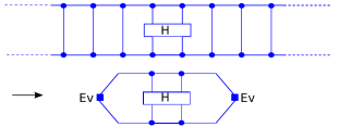
Figure 2: Approximate the energy through the environment matrix, $E$. Note that because the system is translation invariant, we only need to calculate H for two neighboring sites. In 1D, by assuming $M$ to be left-right symmetric, the environment matrices on the left and right will be the same.

In $1D$, the environment tensor method is essentially a variational calculation based on the above matrix-product state, with matrices $M$’s as variational parameters. We use the matrices $M$’s to obtain the average energy (see the top of Fig. 2). We minimize the the average energy to obtain $M$’s.

The calculation of average energy is actually a finite calculation. The key is to use “environment matrix” to capture the contributions from far-away sites. This is graphically shown in the bottom of Fig. 2. As can be seen, there are two environment matrices, one on each side of the $1D$ chain.

So in the actual environment tensor method, we use the matrices $M$’s to obtain the environment matrices $E$, and then use the matrices $M$’s and environment matrices $E$’s to obtain the average energy. We then minimize the average energy to obtain $M$’s (and $E$’s).

Figure 3: A self-consistent condition that environment matrix $E$ must satisfy, where $\lambda$ is a scaling factor. The part enclosed by the shaded area is the so-called double-tensor $T_{b\beta,a\alpha}$.

For fixed matrices $M$’s, the environment matrix could be obtained through iterations. As shown in Figure 3, starting from some random initial values $E_{0}$ that satisfies Tr$E_{0}^{\dagger}E_{0}=1$, we can update the environment matrix using a “double-tensor”, which is formed by two $M$ matrices with physical indices contracted. After applying the “double-tensor”, $E_{0}$ is changed to $\lambda_{1}E_{1}$ where $E_{1}$ satisfies Tr$E_{1}^{\dagger}E_{1}=1$ and $\lambda_{1}$ is a scaling factor. After iterating enough number of times, a final stable “environment matrix” $E_{\infty}=E$ and a final stable scaling factor $\lambda_{\infty}=\lambda$ would be reached. Note that this process, after viewing the environment as a vector and the double-tensor as an operator, is essentially equivalent to picking out the eigenvector with the largest absolute value of the eigenvalues of the double tensor. In this way, for each $M$, we can obtain the corresponding environment matrix $E$ through iterations, and by applying $E$ both on the left and on the right (see Figure 2), we can get the total energy. The variational calculation could then be carried out for different values of $h/J$, and a phase diagram could then be obtained.

More specifically, we require our matrix-product state to have a $\mathbb{Z}_{2}$ symmetry that corresponds to spin up-down flipping, for both the symmetry-breaking and the symmetric phases. So even in symmetry breaking phase, we choose the ground state to be, say, $(\ket{\uparrow\uparrow\dots}+\ket{\downarrow\downarrow\dots})$ when $h/J\to 0$. Note that this is different from traditional symmetry breaking description, where the ground state spontaneously picks one of the ferromagnetic states.

Recall that on-site symmetry of the ground state requires matrices $M$’s to transform in a special way w.r.t. symmetry:Perez-Garcia et al. (2008)

$$\sum_{m^{\prime}}{g_{mm^{\prime}}M^{m^{\prime}}}=e^{i\theta_{g}}U^{\dagger}_{g}M^{m}U_{g}$$ (3)

Here, $m$ is the spin index, matrix $g_{mm^{\prime}}$ represents the on-site symmetry and acts on the spin basis, $\theta$ is a phase factor (set to $0$ in this paper), $U_{g}$ is a unitary matrix acting on internal degrees of freedom, and forms a projective representation of the symmetry group $g$.Pollmann et al. (2010); Chen et al. (2011); Schuch et al. (2011)

For internal dimension $D$ (dimension of $M$) being 2, we can choose $U_{g}=\begin{pmatrix}1&0\\ 0&-1\end{pmatrix}$, then equation (3) reduces to

$$M^{\uparrow}=U^{\dagger}_{g}M^{\downarrow}U_{g},$$ (4)

and we thus have: $M^{\uparrow}=\begin{pmatrix}a&b\\ b&c\end{pmatrix}$ and $M^{\downarrow}=\begin{pmatrix}a&-b\\ -b&c\end{pmatrix}$. Here $M$’s are symmetric because of left-right symmetry, and $a,b,c$ are free variational parameters.

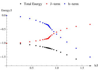
Figure 4: Energy as a function of h/J. The h- and J- terms are also individually plotted in the graph, so the phase transition could be easily spotted at h/J = 0.83. This result is obtained when internal dimension D=2, and we’ve chosen the grid so that sample points are denser close to the transition point.

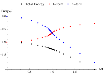
Figure 5: Energy plot when internal dimension increased to D=4. We can see the phase transition point occured around h/J = 0.97, a big improvement from Fig. 4.

With the above symmetry analysis in mind, numerical simulation could be run on our $1D$ Ising model. Following the previous discussion, for each $h/J\in[0,\infty]$ in equation (1), we minimize the energy by varying $M$’s satisfying equation (4). By plotting the two energy terms, a phase diagram is obtained (see Fig. 4). For internal dimension $D=2$, the phase transition occurred at $h/J=0.83$, with an error of $17\%$.

We could easily improve the result by increasing the internal dimension. For internal dimension $D=4$, we can choose $U_{g}$ in (4) to be $\begin{pmatrix}I&0\\ 0&-I\end{pmatrix}$, where $I$ is the $2\times 2$ Identity matrix. The most general symmetric $M$ satisfying (4) has $10$ variational parameters. Following the same variational procedure, we can get the energy plot shown in Fig. 5. The phase transition occurred at $h/J=0.97$, with a mere $3\%$ error.

Note that in both calculations, we used symmetric matrices $M$’s with all real parameters. The typical runtime on a laptop was just a few seconds in both cases.

III Symmetry structure of the environment matrix

From the above plot, we see that there is a phase transition at $h/J\approx 0.83$. To understand the phases on the two sides of the transition, let us choose another basis

$$\tilde{M}^{\uparrow}=WM^{\uparrow}W^{\dagger}=\frac{1}{2}\begin{pmatrix}a+c+2b&a-c\\ a-c&a+c-2b\end{pmatrix}$$

$$\tilde{M}^{\downarrow}=WM^{\downarrow}W^{\dagger}=\frac{1}{2}\begin{pmatrix}a+c-2b&a-c\\ a-c&a+c+2b\end{pmatrix}$$ (5)

where $W=2^{-1/2}\begin{pmatrix}1&1\\ 1&-1\end{pmatrix}$. In the new basis the meaning of the $\tilde{M}$’s is more clear.

When $b=0$, $\tilde{M}^{\uparrow}=\tilde{M}^{\downarrow}$, and the MPS is a pure product state $\otimes(|\uparrow\rangle+|\downarrow\rangle)$ that does not break the $Z_{2}$ symmetry. When $b\neq 0$ and $a=c$, the MPS is a symmetry breaking state of the form $|\Psi\rangle+U|\Psi\rangle$ where $U$ is $Z_{2}$ symmetry transformation. But when $b\neq 0$ and $a\neq c$, what is the nature of the MPS?

To answer such a question, we would like to study the symmetry structure of the environment matrix $E$. We find that, depends on which phase we are in, the symmetry structure of $E$ will be very different.

As we mentioned before, the environment matrix $E$ and the associated scaling factor $\lambda$ is calculated via the iteration (or the self consistent condition) in Fig. 3. In general, there can be many environment matrices $E$ that satisfy the self consistent condition. Here we choose those with largest absolute value of the scaling factor $\lambda$. If there are many environment matrices with the degenerate largest absolute value of the scaling factor, we then choose the environment matrices with minimal “entropy”

$$S=\sum_{i}-s_{i}\ln s_{i},$$ (6)

where $s_{i}$ is the singular values of $E$. This will give us a set of environment matrices $\{E\}$.

Next, we want to point out that environment matrix has only internal indices, so for $E$, the symmetry transformation (3) translates to:

$$E\to U^{\dagger}_{g}\cdot E\cdot U_{g}.$$ (7)

If the $M$’s are invariant under the symmetry transformation (3), then the set of environment matrices $\{E\}$ will be invariant under the above transformation (7).

If the action of transformation (7) is trivial on the set of environment matrices $\{E\}$, then the MPS does not have symmetry breaking. If the action is non-trivial (i.e. generate a permutation of the set $\{E\}$), then the MPS, in general, has a symmetry breaking; but this is not guaranteed.

Figure 6: The entanglement density matrix can be calculated from the environment matrix. (The correct entanglement density matrix should be calculated from the total the environment tensor $E^{0}\otimes E^{0}+E^{1}\otimes E^{1}$.)

The reason for the complication is that there are zero-measure possibilities that some internal bond degrees of freedom completely decouple from the physical degrees of freedom. To fix this problem, we may consider the entanglement density matrix $\rho_{m_{1}m_{2}\cdots,m_{1}^{\prime}m_{2}^{\prime}\cdots}$ defined in Fig. 6. We say two environment matrices are equivalent if they generate the same $\rho_{m_{1}m_{2}\cdots,m_{1}^{\prime}m_{2}^{\prime}\cdots}$. Let us use $\{E\}/\sim$ to denote the equivalent class of the environment matrices. Then if the action (7) is non-trivial on $\{E\}/\sim$, then the MPS has a symmetry breaking.

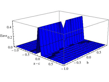
Figure 7: The off-diagonal term in environment matrix is plotted here as a function of $a-c$ and $b$. We can see the delta-function-like behavior when $a=c$. Note the dip at $a=c$ and $b=0$: this point corresponds to the four-fold degeneracy in the double-tensor, which is in the symmetric phase.

With the above general discussion, we now go to our numerical results for internal dimension $D=2$. For the symmetric phase, using the iteration method in Figure 3 and after energy minimization, we obtain a final $E=\begin{pmatrix}s&0\\ 0&t\end{pmatrix}$, which gives an invariant $E$ under eqn (7). As a result, the total environment tensor has a pure tensor product form

$$E^{tot}=E\otimes E,$$ (8)

For the symmetry-breaking phase, after minimizing entropy according to eqn. (6), depending on the initial values of $E$, the iteration method would give either $E^{g_{1}}=\begin{pmatrix}p&p\\ p&p\end{pmatrix}$ or $E^{g_{2}}=\begin{pmatrix}p&-p\\ -p&p\end{pmatrix}$, which transforms into each other under eqn (7). Both of these correspond to environment matrix of the fixed-point wavefunction, as explained later in this section. If we construct the total environment tensor

$$E^{tot}=E^{g_{1}}\otimes E^{g_{1}}+E^{g_{2}}\otimes E^{g_{2}},$$ (9)

then the $\mathbb{Z}_{2}$ symmetry is restored, but now the the total environment tensor does not have a pure tensor product form.

We are now in the position to answer the question raised at the begining of this section. We now know that symmetry-breaking phase is signatured by a non-zero off-diagonal term in the environment matrix. As shown in Fig. 7, if we plot this off-diagonal term as a function of $a-c$ and $b$ in $M$ (see eqn (III)), then we see that the system is only in symmetry breaking state when $a=c$ and $b\neq 0$. So when $b\neq 0$ and $a\neq c$, the state is in the symmetric phase.

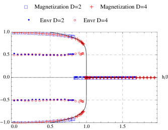
Figure 8: A plot of magnetization and the “fixed-point” order paramter as a function of $h/J$. When we increase the internal dimension, we get a more accurate phase transition point. In both cases, we get a first-order phase transition. When internal dimension $D=2$, order parameter is just the off-diagonal term of the environment matrix (represented by blue dots). When $D=4$, order parameter is the norm of the $2\times 2$ off-diagonal block in the environment matrix (represented by red circles). The black line curve is $\langle\sigma_{i}^{z}\rangle=\pm(2-2h)^{1/8}$.

Here we’ve also plotted the magnetization as a function of $h/J$ in Fig. 8. Note that in the graph, we get a first-order phase transition for both $D=2$ and $D=4$. This is because we required our matrices $M$’s in the MPS to have the $\mathbb{Z}_{2}$ symmetry (recall eqn. (III)). This symmetry requirement favors the symmetric phase, because symmetry-breaking phase requires $a=c$, so $M$ is block-diagonalized, reducing its effective internal dimension. Thus the phase transition point is shifted leftwards, leading to a first-order transition. As we increase the internal dimension, we expect the phase transition point to approach $h/J=1$ from the left.

In Fig. 8, we’ve also plotted the order parameter as a function of $h/J$. Note that these “order parameters” do not vary as we change $h/J$. This is because the environment matrix is obtained from enough iterations that it really corresponds to the fully renormalized wavefunction. The order parameter obtained from the environment matrix then corresponds actually to the order parameter at the fixed point, thus is always the same until hitting the phase transition point.

IV Detecting phases of MPS without knowing the transformation property of the matrices

In the above, we have assumed that the matrices in the MPS has the symmetry and studied how to use the symmetry breaking of the environment matrix to detect the spontaneous symmetry breaking in MPS. However, in many calculations, such as the density-matrix-renormalization-group (DMRG) calculation, the resulting matrices in the MPS do not have the symmetry in the symmetry breaking phase, and in general we do not even know how the matrices transform under the symmetry transformation (since we do not know how the internal indices should transform under the symmetry). In this section, we will discuss how to detect the spontaneous symmetry breaking in MPS, without knowing how the matrices in the MPS transforms under the symmetry transformation.

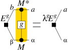
Figure 9: A self-consistent condition that environment matrix $E^{g}$ must satisfy, where $\lambda^{g}$ is a scaling factor. The part enclosed by the shaded area is the symmetry twisted double-tensor $T^{g}_{b\beta,a\alpha}$.

Assume we have already obtained the matrices in the MPS. We first calculate the environment matrix $E$ and the scaling factor $\lambda$ using Fig. 3. In general, the environment matrix $E$ is unique even in the symmetry breaking state, since the matrices in the MPS obtained from DMRG in general already break the symmetry. Next, we insert the symmetry transformation $g$ (see (3)) in the double-tensor to obtain a twisted double-tensor. The corresponding twisted environment matrix is denoted as $E^{g}$ and the twisted scaling factor as $\lambda^{g}$ (see Fig. 9).

If $|\lambda^{g}|<|\lambda|$, then the corresponding MPS have a spontaneous symmetry breaking. In fact, there is a more direct way to detect symmetry breaking. Let $P$ and $P^{g}$ be the matrices defined via the $n^{\text{th}}$ power of double-tensor (where $T$ and $T^{g}$ are viewed as matrices)

$$P_{ab,\alpha\beta}=T^{n}_{b\beta,a\alpha},\ \ \ \ \ P^{g}_{ab,\alpha\beta}=(T^{g})^{n}_{b\beta,a\alpha}.$$ (10)

If $P$ and $P^{g}$ have different singular values in large $n$ limit, then the corresponding MPS break the symmetry explicitly.

If $|\lambda^{g}|=|\lambda|$, then the two environment matrices $E^{g}$ and $E$ are related by the symmetry transformation (see (3))

$$E=E^{g}U_{g},\ \ \ \ \text{ or }\ \ \ \ E^{-1}E^{g}=U_{g}^{\dagger}.$$ (11)

In fact, we have

$$E=U_{g}^{\dagger}EU_{g}$$ (12)

If $U_{g}$ forms a projective representation of the symmetry group $G$, then the corresponding MPS does not break the symmetry and has a non-trivial SPT order protected by the on-site symmetry. If $U_{g}$ forms a 1D representation of the symmetry group $G$, then the corresponding MPS does not break the symmetry and has a non-trivial SPT order protected by translation symmetry (and the on-site symmetry).

Let us apply the above approach to a MPS state of spin-1 chian, where the matrix $M^{l}$, $l=x,y,z$ are given by the Pauli matrices: $M^{l}=\sigma^{l}$. The double-tensor is given by (see Fig. 3)

$$T_{b\beta,a\alpha}=\sigma^{x}_{ba}\sigma^{x}_{\beta\alpha}-\sigma^{y}_{ba}\sigma^{y}_{\beta\alpha}+\sigma^{z}_{ba}\sigma^{z}_{\beta\alpha}$$ (13)

The action of the double-tensor $T_{b\beta,a\alpha}$ on the environment matrix $E_{b\beta}\to T_{b\beta,a\alpha}E_{a\alpha}$ can be written in a matrix form

$$E\to\sum_{l}\sigma^{l}E\sigma^{l}.$$ (14)

We see that $E=2^{-1/2}\sigma^{0}$ (the 2-by-2 identity matrix) is the non-degenerate environment matrix with $\lambda=3$.

Now, let us show that the MPS has a $Z_{2}^{x}\times Z_{2}^{z}$ symmetry where $Z_{2}^{x}$ is generated by $R_{x}$ – the $180^{\circ}$ spin rotation in $S^{x}$-direction and $Z_{2}^{z}$ is generated by $R_{z}$ – the $180^{\circ}$ spin rotation in $S^{z}$-direction. Under the symmetry twists $R_{x}$ and $R_{z}$, the corresponding double-tensors are

$$T^{R_{x}}_{b\beta,a\alpha}=-\sigma^{x}_{ba}\sigma^{x}_{\beta\alpha}-\sigma^{y}_{ba}\sigma^{y}_{\beta\alpha}+\sigma^{z}_{ba}\sigma^{z}_{\beta\alpha}$$

$$T^{R_{z}}_{b\beta,a\alpha}=+\sigma^{x}_{ba}\sigma^{x}_{\beta\alpha}-\sigma^{y}_{ba}\sigma^{y}_{\beta\alpha}-\sigma^{z}_{ba}\sigma^{z}_{\beta\alpha}.$$ (15)

The corresponding twisted environment matrices are given by

$$E^{R_{x}}=2^{-1/2}\sigma^{x},\ \ \ \ E^{R_{z}}=2^{-1/2}\sigma^{z}.$$ (16)

with $\lambda^{R_{x}}=\lambda^{R_{z}}=-3$. We see that

$$U_{R_{x}}=\sigma^{x},\ \ \ \ U_{R_{z}}=\sigma^{z},$$ (17)

Since $|\lambda^{R_{x}}|=|\lambda^{R_{z}}|=|\lambda|$ and

$$E=U_{R_{x}}^{\dagger}EU_{R_{x}},\ \ \ \ E=U_{R_{z}}^{\dagger}EU_{R_{z}},$$ (18)

we found that the $Z_{2}^{x}\times Z_{2}^{z}$ symmetry is not broken. We also see that $U_{R_{x}},U_{R_{z}}$ generate a projective representation of $Z_{2}^{x}\times Z_{2}^{z}$. So the MPS is a SPT state protected by $Z_{2}^{x}\times Z_{2}^{z}$.

V A tensor network approach for 1D model

In this section, we are going to use an infinite time-evolving block decimation (iTEBD) approachVidal (2007b) to study 1D models, such as the transverse Ising model (1). We are going study symmetry breaking by testing if $|\lambda^{g}|=|\lambda|$ or $|\lambda^{g}|<|\lambda|$.

V.1 The iTEBD method

The iTEBD method is a tensor network version of the DMRG approach. The fundamental idea behind the iTEBD method is to use imaginary time evolution to get the ground state of a two-body Hamiltonian, and to use Singular Value Decomposition (SVD) to control the internal dimensions.

Figure 10: Applying imaginary time evolution in a layered structure.

Consider any $1D$ Hamiltonian with only nearest-neigbour interactions, we can always separate it into two parts, labeled by $H_{A}$ and $H_{B}$:

$$H =\sum_{i}H_{i,i+1}=\sum_{i\in odd}H_{i,i+1}+\sum_{i\in even}H_{i,i+1}$$

$$=H_{A}+H_{B}.$$ (19)

This way, either $H_{A}$ or $H_{B}$ would have no overlapping terms within itself. When the time step $\delta t$ is very tiny, we have:

$$e^{-\delta tH}\approx e^{-\delta tH_{A}}e^{-\delta tH_{B}}\equiv W.$$ (20)

We could then apply imaginary-time evolution layer by layer, as shown in Fig. 10. Now within each layer, time-evolution only operates on non-overlapping neighboring sites. Thus the entire problem reduces to a two-site problem.

Figure 11: Time-evolution on two sites. Step $1$: apply time-evolution operator. Step $2$: apply SVD and truncate the singular matrix to only contain $D$ largest singular values ($\bar{S}$ denotes the singular matrix after truncation). Step $3$: seperate the singular values into the two sites.

The two-site time-evolution is done through Singular Value Decomposition, see Fig. 11. We first apply the time-evolution operator (labeled by $W_{i,i+1}$) on two sites, resulting in a rank-$4$ tensor, $T_{m^{\prime}\alpha,k^{\prime}\gamma}$:

$$T_{m^{\prime}\alpha,k^{\prime}\gamma}=W_{m^{\prime}k^{\prime},mk}A^{m}_{\alpha\beta}B^{k}_{\beta\gamma}.$$ (21)

Then we do SVD to split the rank-$4$ tensor:

$$T_{m^{\prime}\alpha,k^{\prime}\gamma}=U_{m^{\prime}\alpha,\beta}S^{\prime}_{\beta\lambda}V_{k^{\prime}\gamma,\lambda}.$$ (22)

Note that after applying SVD, the internal dimension has grown on the inner link. We could get back our original internal dimension by keeping only the $D$ largest singular values of $S^{\prime}$. We’ll call the truncated matrix $\bar{S}$. Finally, we absorb diagnomal matrix $\bar{S}$ into the two on-site matrices, thus completing one step of evolution:

$$\bar{A}^{m^{\prime}}_{\alpha\beta}=U_{m^{\prime}\alpha,\beta}\sqrt{\bar{S}_{\beta}},\ \ \bar{B}^{k^{\prime}}_{\beta\gamma}=V_{k^{\prime}\beta,\gamma}\sqrt{\bar{S}_{\beta}}.$$ (23)

This completes one step in time evolution.

One improvement can be made on the above time-evolution step. Note that in the truncation process above, we implicitly assumed that all bond indices are equally important; however, we know that’s not the case. The “environment indices” $\alpha,\gamma$ do not contribute equally, and their weights could be naturally included by using the singular values $S_{\alpha},S_{\gamma}$ from the previous time-evolution step. (This is because in the previous step, $\alpha$ and $\gamma$ were inner link indices, and each index naturally carries a weight according to the previous step of SVD.)

Thus the improved time-evolution step works as follows: $1.$ First, we scale the “environment indices” using singular values $S_{\alpha}$ obtained from last step:

$$A^{m}_{\alpha\beta}\rightarrow\sqrt{S_{\alpha}}A^{m}_{\alpha\beta},\ \ B^{m}_{\beta\gamma}\rightarrow\sqrt{S_{\gamma}}A^{m}_{\beta\gamma}.$$ (24)

$2.$ Then apply the time-evolution step described before. $3.$ Lastly, we scale the “enviornment indices” back, by doing the following:

$$\bar{A}^{m}_{\alpha\beta}\rightarrow\sqrt{S^{-1}_{\alpha}}\bar{A}^{m}_{\alpha\beta},\ \ \bar{B}^{m}_{\beta\gamma}\rightarrow\sqrt{S^{-1}_{\gamma}}\bar{B}^{m}_{\beta\gamma}.$$ (25)

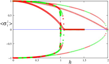
Figure 12: The three up-down symmetric curves describe the magnetization of transverse Ising model $\langle\sigma^{z}_{i}\rangle$ as a function of $h$ with $J=1$. The “+” points are for internal dimension $D=1$, “$+\hskip-7.20709pt\times$” for $D=2$, and filled-box for $D=10$. The other three curves describe $\frac{|\lambda|-|\lambda_{g}|}{|\lambda|}$. The “$\times$” points are for $D=1$, “$\square$” for $D=2$, and open-circle near (1,0) are for $D=10$. The line curve is $\langle\sigma^{z}_{i}\rangle=\pm(2-2h)^{1/8}$.

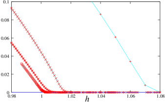
Figure 13: The difference of the scaling factors $\frac{|\lambda|-|\lambda_{g}|}{|\lambda|}$ of transverse Ising model as a function of $h$ with $J=1$. The “+” points are for $D=2$, “$\times$” for $D=4$, “$+\hskip-7.20709pt\times$” for $D=8$, and “$\square$” for $D=16$.

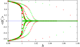
Figure 14: The magnetization of transverse Ising model $\langle\sigma^{z}_{i}\rangle$ as a function of $h$ with $J=1$. The “+” points are for $D=2$, “$\times$” for $D=4$, “$+\hskip-7.20709pt\times$” for $D=8$, “$\square$” for $D=16$, and “$\blacksquare$” for $D=32$. The line curve is $\langle\sigma^{z}_{i}\rangle=\pm(2-2h)^{1/8}$.

V.2 The iTEBD results for transverse Ising model

After applying the imaginary-time evolution steps described above, we will eventually obtain the tensor that describes the ground state wave function very well. The next issue is to identify the symmetry breaking order and/or SPT order in the ground state, using the method discussed before.

For the transverse Ising model, Fig. 12 describes the calculated $\frac{|\lambda|-|\lambda_{g}|}{|\lambda|}$ and the magnetization $\langle\sigma^{z}_{i}\rangle$, using the iTEBD approach with various $D$. Fig. 13 and Fig. 14 are the results near the transition point. The transition point is found to be $h_{c}\approx 1.08$ for $D=2$, $h_{c}\approx 1.0188$ for $D=4$, $h_{c}\approx 1.0101$ for $D=8$, $h_{c}\approx 1.0047$ for $D=16$, and $h_{c}\approx 1.0015$ for $D=32$. The exact transition point is at $h_{c}=1$. We see that “order parameter” $\frac{|\lambda|-|\lambda_{g}|}{|\lambda|}$ works very well, in identify symmetry breaking transitions.

V.3 The iTEBD calculation of 1D model with symmetry-breaking and/or SPT orders

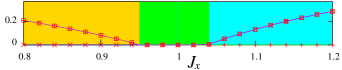
Figure 15: $\frac{|\lambda|-|\lambda_{g}|}{|\lambda|}$ for the spin-1 model as a function of $J_{x}$ with $J_{y}=J_{z}=1,J_{zz}=0.4$, calculated by the iTEBD method with $D=8$. The “+” points are for symmetry twist $g=R_{x}$, “$\times$” for $g=R_{y}$, and “$\square$” for $g=R_{z}$. When $\frac{|\lambda|-|\lambda_{g}|}{|\lambda|}=0$, the corresponding symmetry $g$ is not broken. We see that the phase near $J_{x}=1$ has the full symmetry. The phase for smaller $J_{x}$ has only the $R_{y}$ symmetry. The phase for larger $J_{x}$ has only the $R_{x}$ symmetry.

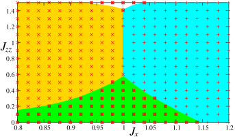
Figure 16: The phase diagram for the spin-1 model in $J_{x}$-$J_{zz}$ plane, with $J_{y}=J_{z}=1$, calculated by the iTEBD method with $D=8$. The points mark which $\frac{|\lambda|-|\lambda_{g}|}{|\lambda|}=0$. The “+” points are for symmetry twist $g=R_{x}$, “$\times$” for $g=R_{y}$, and “$\square$” for $g=R_{z}$. The green shaded area and the white area at the top have the full $R_{x},R_{y},R_{z}$ symmetry. The gold shaded area has only the $R_{y}$ symmetry, and the blue shaded area has only the $R_{x}$ symmetry.

In this section, we are going to use the iTEBD appraoch to study spin-1 model with $Z_{2}^{x}\times Z_{2}^{z}$ symmetry:

$$H=\sum_{i}[J_{x}S_{i}^{x}S_{i+1}^{x}+J_{y}S_{i}^{y}S_{i+1}^{y}+J_{z}S_{i}^{z}S_{i+1}^{z}+J_{zz}(S_{i}^{z})^{2}]$$ (26)

The $Z_{2}^{x}$ is generated by $180^{\circ}$ spin-rotation $R_{x}$ around the $S_{x}$ axis. The $Z_{2}^{z}$ is generated by $180^{\circ}$ spin-rotation $R_{z}$ around the $S_{z}$ axis. The $R_{x}R_{z}=R_{y}$ is the $180^{\circ}$ spin-rotation around the $S_{y}$ axis.

We choose $D=8$ and calculated the tensor $M^{m}_{\alpha\beta}$ for the ground state. To determine if $M^{m}_{\alpha\beta}$ describes a symmetry breaking state or not, it is not correct to directly test if $M^{m}_{\alpha\beta}$ has the symmetry or not. This is because even when $M^{m}_{\alpha\beta}$ is not invariant under any symmetry transformation of the form (3), $M^{m}_{\alpha\beta}$ can still describe a symmetric state.

So to determine symmetry of the ground state, we instead calculated the quantity $\frac{|\lambda|-|\lambda_{g}|}{|\lambda|}$ for symmetry twists $g=R_{x},R_{y},R_{z}$ (see Fig. 15). We determined the phase diagram by examine where and which $\frac{|\lambda|-|\lambda_{g}|}{|\lambda|}$ vanishes. The gold shaded area in Fig. 16 only has the $R_{x}$ symmetry, since only $\frac{|\lambda|-|\lambda_{R_{x}}|}{|\lambda|}=0$. The blue shaded area in Fig. 16 only has the $R_{y}$ symmetry since only $\frac{|\lambda|-|\lambda_{R_{y}}|}{|\lambda|}=0$. The green shaded area and the white area have $\frac{|\lambda|-|\lambda_{g}|}{|\lambda|}=0$ for $g=R_{x},R_{y},R_{z}$ and have the full $R_{x},R_{y},R_{z}$ symmetry. In fact the green area is a phase with a non-trivial SPT order (the Haldane phase).

VI Application to 2D model with symmetry breaking transition

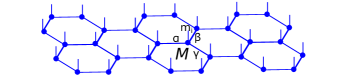
Figure 17: A tensor-network state. All the physical sites are represented by dots, physical degrees of freedom by vertical lines, and internal degrees of freedom by in-plane links.

Now we want to generalize the above simple picture to $2D$. Consider the transverse Ising model on an infinite honeycomb lattice, with spins living on vertices. The Hamiltonian remains the same as equation (1). Since the ground state of a gapped system in $2D$ could be faithfully described by a tensor-network state, Xiang et al. (2001); Legeza and Solyom (2004); Vidal et al. (2003); Srednicki (1993); Plenio et al. (2005) for a translation invariant system, we have (see Figure 17):

$$\Ket{\Psi}=\sum_{\{m_{i}\}}\sum_{\{\alpha,\beta,\gamma\}}\text{tTr}[\otimes_{i}M_{\alpha,\beta,\gamma}^{m_{i}}]\Ket{\{m_{i}\}}$$ (27)

where tensors $M$’s are again labeled by the physical degrees of freedoms $m_{i}$, and tTr (tensor trace) contracts over all internal degrees of freedom on connected links labeled by $\alpha,\beta$ and $\gamma$. Again, we want to do variational calculations with a simple picture involving the total environment tensor $E^{tot}$, which now consists of four environment matrices, see Figure 18.

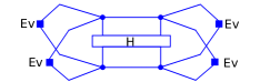
Figure 18: The average energy with total environment tensor $E^{tot}$ in $2D$. Here, $E^{tot}$ consists of four environment matrices, surrounding the two physical sites.

The key question now is how do we obtain a good environment matrix, as we did in $1D$ (recall Figure 3)? Here we introduce a simple yet powerful iteration process: assume we have a three-fold rotational symmetry for tensor $M$, then the iteration needs two input matrices, and gives out only one output, see Figure 19. As before, after enough numbers of iterations, we would reach a final stable “environment matrix”.

Figure 19: The self-consistent iteration process for environment in $2D$.

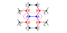
Figure 20: The iteration process on Bethe lattice. Note that this is a top-down view, and we have only shown one layer of tensor-network state. Starting from an environment surrouding $C$ tensor, we could iterate to get environment for $B$, and then to $A$. The circled region is the region of interest.

It might be surprising, at first sight, why such a naive iteration process would give a reliable environment matrix. The key however is to realize that this iteration actually gives an environment matrix for the infinite Bethe lattice, which is a very good first approximation for our honeycomb lattice (see Figure 20). As shown in the graph, the iteration process is actually equivalent to a self-consistent update for a large cluster of lattice points, and thus its legitimacy.

Just like in the $1D$ case, here we would also like to require our tensor-product state to have a $\mathbb{Z}_{2}$ symmetry corresponding to the spin up-down symmetry. Similar to the matrix-product state, on-site symmetry of the ground state also requires tensor $M$ in the tensor-network state to transform in a special way:

$$\sum_{m^{\prime}}{g_{mm^{\prime}}M_{\alpha,\beta,\gamma}^{m^{\prime}}}=e^{i\theta_{g}}\sum_{\alpha^{\prime},\beta^{\prime},\gamma^{\prime}}{M_{\alpha^{\prime},\beta^{\prime},\gamma^{\prime}}^{m}U_{g}^{\alpha\alpha^{\prime}}U_{g}^{\beta\beta^{\prime}}U_{g}^{\gamma\gamma^{\prime}}}.$$ (28)

This is just a tensor generalization of condition (3). As before, $m$ is the physical spin label, $g_{mm^{\prime}}$ represents the on-site symmetry and acts in the spin space, $U_{g}$ forms a projective representation of the symmetry group $g$, and is a unitary matrix acting on internal degrees of freedom labeled by $\alpha,\beta$ and $\gamma$.

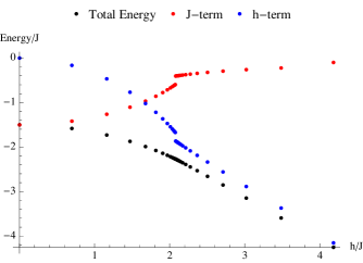
Figure 21: Energy as a function of h/J for the $2D$ transverse Ising model. As in the $1D$ case, h- and J- terms are individually plotted in the graph as well. We can see from the graph that our simulation shows a weak first-order phase transition, with phase transition point at $h/J=2.09$.

For internal dimension of $D=2$, we can choose $U_{g}=\begin{pmatrix}1&0\\ 0&-1\end{pmatrix}$. The most general symmetric tensor $M^{m_{i}}_{\alpha,\beta,\gamma}$ satisfying eqn. (28) has $4$ variational parameters and looks like the following:

$$M^{\uparrow,\alpha=1}_{\beta,\gamma} =\begin{pmatrix}a&b\\ b&c\end{pmatrix}\ \ M^{\uparrow,\alpha=2}_{\beta,\gamma}=\begin{pmatrix}b&c\\ c&d\end{pmatrix},$$

$$M^{\downarrow,\alpha=1}_{\beta,\gamma} =\begin{pmatrix}a&-b\\ -b&c\end{pmatrix}\ \ M^{\uparrow,\alpha=2}_{\beta,\gamma}=\begin{pmatrix}-b&c\\ c&-d\end{pmatrix}.$$ (29)

Here we again assume $M$’s to be symmetric, because of rotational symmetry.

With the above $M$ tensors, numerical simulation could again be run on the $2D$ Ising model. Following what we did in $1D$, we vary $h/J$ in equation (1) and minimize the energy for each value of $h/J$. By plotting the two energy terms, a phase diagram could also be obtained (see Fig. 21). For internal dimension $D=2$, the phase transition point occured at $h/J=2.09$, which was within $2\%$ error from Quantum Monte Carlo prediction of $h/J=2.13$.Blote and Deng (2002) The typical runtime on a laptop was just a few seconds. If we increase the internal dimension to $D=4$ and use a completely symmetric tensor with $10$ variational paramters, then we get a phase transition point at $h/J=2.12$, within $1\%$ error from the aforementioned Quantum Monte Carlo calculation. Here all variational parameters are real.

Following what we did in $D=1$, here we would also like to comment on the symmetry structure of the environment matrix $E$. Recall that $E$ is obtained through iterations (or self consistent condition) in Fig. 19, which picks out the $E$ with the largest absolute value of scaling factor $\lambda$. One important difference/simplification in $2D$ is that unlike in $1D$, in general, we do not have any degeneracies for $E$ through the iteration equation (Fig. 19), since the equation is non-linear. Thus in general $E$ obtained is unique, and we do not need eqn. (6) to fix the basis.

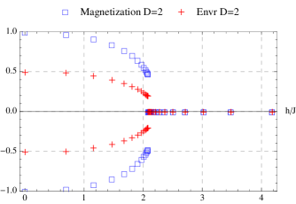
Figure 22: Magnetization and order parameter as a function of h/J for the $2D$ transverse Ising model. When $D=2$, the order parameter plotted (represented by red crosses) is ${p/(s+t)}$, which goes to zero in the symmetric phase.

With the above discussion, we can go into the symmetry structure for our environment matrix $E$ (See Fig. 22). For internal dimension being 2, using the iteration method mentioned above and after energy minimization, we have in the symmetric phase $E=\begin{pmatrix}s&0\\ 0&t\end{pmatrix}$, which gives an invariant $E$ under eqn. (7). As a result, the total environment tensor is just the direct-product of them:

$$E^{tot}=E\otimes E\otimes E\otimes E.$$ (30)

As for the symmetry breaking phase, depending on the initial values of E, we get either $E^{g_{1}}=\begin{pmatrix}\tilde{s}&p\\ p&\tilde{t}\end{pmatrix}$ or $E^{g_{2}}=\begin{pmatrix}\tilde{s}&-p\\ -p&\tilde{t}\end{pmatrix}$, which transforms into each other under eqn. (7). If we construct the total environment tensor

$$E^{tot}=\sum_{g}{E^{g}\otimes E^{g}\otimes E^{g}\otimes E^{g}},$$ (31)

then the $\mathbb{Z}_{2}$ symmetry is restored, but now again the total environment tensor does not have a pure tensor product form, as was the case in $1D$.

VII Application to 2D model with topological order

We now move on to the non-trivial example of Toric-Code model in a B-field, with spins living on links of an infinite $2D$ honeycomb lattice. The Hamiltonian is as follows:

$$H=-A\sum_{v}\prod_{i\in v}\sigma_{i}^{z}-B\sum_{p}\prod_{j\in p}\sigma_{j}^{x}-h\sum_{k}\sigma_{k}^{z}$$ (32)

where $\sigma$’s are the usual Pauli matrices. We will first consider the phase diagram by fixing $A\to\infty$ and varying $h/B$ between $[0,\infty]$. When $h/B=0$, we have the original Toric-Code model, whose ground state is an equal-weight superposition of all closed loops of down-spins (in the background of up-spins). When $h/B\to\infty$, we have the spin-polarized state where all spins are pointing up.

Later in this section, we will also consider the case when $h/B\to-\infty$ so the ground state is the fully packed loop state, which is an equal weight superposition of all loop configurations that are fully packed (every vertex has a loop passing through). The question of whether the fully packed loop state has topological order or not will then be explored.

Figure 23: Tensor-product state with spins living on links. Here physical sites are represented by dots.

As in the previous example, we now try to use a tensor-network state to represent the ground state of the above Hamiltonian. Here since all spins live on links of the lattice, we will need two tensors $T$ and $M$ to represent our variational ground state (see Figure 23):

$$\Ket{\Psi}=\sum_{\{m_{l}\}}\sum_{\{\alpha,\beta,\gamma,\delta,\eta\}}\text{tTr}[\otimes_{v}T_{\alpha,\beta,\gamma}\otimes_{l}M_{\delta,\eta}^{m_{l}}]\Ket{\{m_{l}\}}$$ (33)

where $v$ labels different vertices, $l$ labels different links, $\alpha,\beta,\gamma,\delta,\eta$ label internal degrees of freedom, $m_{l}$ label physical degrees of freedom of link $l$, and tTr contracts over all connected internal indices. Note that due to the $B$ term in the Hamiltonian 32, we will need to include an entire plaquette in our variational calculation, as shown in Figure 24.

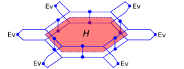
Figure 24: Variational energy for Toric-Code model in a B-field.

Now we start by introducing our tensor ansatz in the simple case of internal dimension $2$. In order to enforce the condition that $A\to\infty$ and the rotational symmetry of the system, we need the following tensors $T$ and $M$:

$$T_{\alpha,\beta,\gamma}= \begin{cases}1,&if\ \alpha=\beta=\gamma=0;\\ x,&else\ if\ \alpha+\beta+\gamma=0\ (\text{mod}\ 2);\\ 0,&\text{otherwise};\end{cases}$$

$$M_{\delta,\eta}^{\uparrow}= \begin{pmatrix}1&0\\ 0&0\end{pmatrix},\ \ M_{\delta,\eta}^{\downarrow}=\begin{pmatrix}0&0\\ 0&1\end{pmatrix}.$$ (34)

where spin-up and spin-down’s are labeled by arrows. Note that when $x=1$, it represents the regular Toric-Code ground stateGu et al. (2009), whereas when $x=0$, it represents the all-spins-up state.

Before going into our variational calculations, we first note that our model in equation (32) could be mapped into a transverse Ising model by introducing a new plaquette spin operator $\mu_{p}$, where spins live on the plaquettes and $p$ is the plaquette label.Trebst et al. (2007) By doing the following mapping: $\prod_{j\in p}\sigma_{j}^{x}\to\mu_{p}^{x}$, $\sigma_{i}^{z}\to\mu_{p}^{z}\mu_{p^{\prime}}^{z}$, and consider only the $A\to\infty$ sector, our Hamiltonian reduces to:

$$H=-B\sum_{p}\mu_{p}^{x}-h\sum_{<p,p^{\prime}>}\mu_{p}^{z}\mu_{p^{\prime}}^{z},$$ (35)

which is the familiar transverse Ising model. Note that this Ising model is now on a $2D$ triangular lattice.

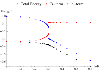
Figure 25: Energy as a function of h/B for the $2D$ Toric Code model in a magnetic field. Here we only plotted the region when $h/B>0$. We can see from the graph that our simulation shows a weak first-order phase transition, with phase transition point at $h/J=0.3$.

With the above tensor network ansatz, we could run our variational scheme on the Toric-Code model. Just like in the Ising model cases, we vary $h/B$ in eqn (32) (recall that we hold $A\to\infty$) and minimize the energy for each value of $h/B$. The environment tensor was calculated in the same way as before (See Fig. 19). The only difference here is that since the Hamiltonian (32) have a six-body interaction term, we have to include more sites into our mean-field calculation(See Figure 24). By plotting the two energy terms as a function of $h/B$, we get a phase diagram, which is plotted in Fig. 25. For internal dimension $D=2$, we got a phase transition point at $B/h=3.33$, with an error of $30\%$ to the Quantum Monte Carlo result of $B/h=4.768$.Blote and Deng (2002) This is not surprising as we only have one variational parameter. With internal dimension of $3$ and only two variational parameters, our result quickly improved to a phase transition point at $B/h=4.407$, with an error of less than $8\%$ to the Quantum Monte Carlo result. Note that the Quantum Monte Carlo value was obtained on the mapped equivalent model (see equation (35)) on a $2D$ triangular lattice.

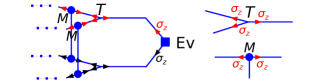
Figure 26: Internal $\mathbb{Z}_{2}$ symmetry of the tensors $T$ and $M$ for our Toric-Code model. Here $T$ has a $\sigma_{z}\otimes\sigma_{z}\otimes\sigma_{z}$ symmetry, and $M$ has a $\sigma_{z}\otimes\sigma_{z}$ symmetry, both of which square to identity. Note that this symmetry transformation could independently act on top and bottom layers of the tensor-network, thus the environment matrix transforms under a $\mathbb{Z}_{2}\times\mathbb{Z}_{2}$ group.

Now in order to understand the above result better and to further explore the case when $h/B<0$, we need to understand the symmetry structure of both our tensor-product state and the environment tensor obtained. Note here that although the ground state doesn’t have a physical $\mathbb{Z}_{2}$ symmetry, the tensor ansatz $T$ and $M$ (VII) still need to have an internal $\mathbb{Z}_{2}$ symmetry, namely the “necessary symmetry condition”Chen et al. (2010b) (See Figure 26):

$$T_{\alpha,\beta,\gamma} =\sum_{\alpha^{\prime},\beta^{\prime},\gamma^{\prime}}{T_{\alpha^{\prime},\beta^{\prime},\gamma^{\prime}}\sigma_{z}^{\alpha\alpha^{\prime}}\sigma_{z}^{\beta\beta^{\prime}}\sigma_{z}^{\gamma\gamma^{\prime}}}$$

$$M_{\delta,\eta}^{m_{l}} =\sum_{\delta^{\prime},\eta^{\prime}}{M_{\delta^{\prime},\eta^{\prime}}\sigma_{z}^{\delta\delta^{\prime}}\sigma_{z}^{\eta\eta^{\prime}}}.$$ (36)

Here, the internal symmetry is represented by $\sigma_{z}\otimes\sigma_{z}\otimes\sigma_{z}$ for tensor $T$, and $\sigma_{z}\otimes\sigma_{z}$ for tenor $M$, where $\sigma_{z}$ is the Pauli matrix. Since both symmetry actions square to identity, we refer to the above internal symmetry as a $\mathbb{Z}_{2}$ symmetry.

The physical reason for tensor ansatz to have the above “necessary symmetry condition” is that we want to make sure local variations of the tensors correspond to local perturbations of the Hamiltonian. Tensors that violates the above condition correspond to non-local perturbation in their Hamiltonian and thus can not be used to describe physical phase transitions Chen et al. (2010b).

It’s easy to check that tensors in equation (VII) have the above symmetry. We would then like to ask, with the $T$ and $M$ tensors satisfying eqn (VII), what is the symmetry structure of the environment matrix? Note that unlike the Ising model, here the internal symmetry of the two layers of our tensor-network can act independently, as shown in Figure 26. Thus the environment matrix no longer transforms under eqn (7), but transforms under a $\mathbb{Z}_{2}\times\mathbb{Z}_{2}$ group:

$$E\to U_{g}^{\dagger}\cdot E,\ \ or\ \ E\cdot U_{g},\ \ or\ \ U_{g}^{\dagger}\cdot E\cdot U_{g}.$$ (37)

As in the Ising model, we expect that in different phases, the environment matrices $E$’s are either invariant under the above transformation, or undergoes a permutation.

Our numerical result indeed shows the above feature. When internal dimension $D=2$, we use the tensor ansatz in eqn (VII) and iteration process (see Fig. 19) to get the environment matrix $E$. In the confined phase (including spin-polarized state), we obtain $E=\begin{pmatrix}1&0\\ 0&0\end{pmatrix}$, which is invariant under eqn. (37). As a result, the total environment tensor is just the direct product of them:

$$E^{tot}=E\otimes E\otimes E\otimes E\otimes E\otimes E.$$

In the deconfined phase (including string-net state), however, we have either $E^{g_{1}}=\begin{pmatrix}s&0\\ 0&t\end{pmatrix}$ or $E^{g_{2}}=\begin{pmatrix}s&0\\ 0&-t\end{pmatrix}$, which transforms into each other under eqn. (37). We could again construct a total environment tensor

$$E^{tot}=\sum_{g}{E^{g}\otimes E^{g}\otimes E^{g}\otimes E^{g}\otimes E^{g}\otimes E^{g}}$$

that respects the $\mathbb{Z}_{2}\times\mathbb{Z}_{2}$ symmetry, but it does not have a pure tensor product form, as was the case for Ising model.

In doing the above, we have really constructed a numerical way to detect topological orders. In the particular case above, $\mathbb{Z}_{2}$ topological order is signatured by a “symmetry breaking” in the environment matrix, which breaks the original $\mathbb{Z}_{2}\times\mathbb{Z}_{2}$ symmetry of $E$ (see eqn (37)) down to $\mathbb{Z}_{2}$ (see eqn (7)).

With this realization, a natural question to ask is: if we now consider negative magnetic field with $h/B\to-\infty$, will the fully packed loop state has $\mathbb{Z}_{2}$ topological order? To answer this question, let us first write down the ground state wave function of the fully packed loop state in tensor form:

$$T_{\alpha,\beta,\gamma}= \begin{cases}0,&if\ \alpha=\beta=\gamma=0;\\ 1,&else\ if\ \alpha+\beta+\gamma=0\ (\text{mod}\ 2);\\ 0,&\text{otherwise};\end{cases}$$

$$M_{\delta,\eta}^{\uparrow}= \begin{pmatrix}1&0\\ 0&0\end{pmatrix},\ \ M_{\delta,\eta}^{\downarrow}=\begin{pmatrix}0&0\\ 0&1\end{pmatrix}.$$ (38)

Note the difference between this and eqn (VII): here we require loops to cover each vertex, so $T_{0,0,0}=0$.

Now to see whether this state has $\mathbb{Z}_{2}$ topological order or not, all we need to do is to calculate its environment matrix through iteration (see Fig. 19). Depending on the initial condition, we obtain either $E^{g_{1}}=\begin{pmatrix}0.38&0\\ 0&0.62\end{pmatrix}$ or $E^{g_{2}}=\begin{pmatrix}0.38&0\\ 0&-0.62\end{pmatrix}$, which again transforms into each other under eqn (37). This means that we are still in the deconfined phase, and packed loop state has $\mathbb{Z}_{2}$ topological order.

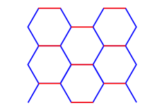
Figure 27: The above graph shows a “string crystal” state, where blue lines represent spin-downs forming vertical strings, and red lines represent spin-ups forming the background.

One may worry that the simple test above would fail to differentiate the “string crystal” state (see Fig. 27) where string configuration is stationary, from the fully packed loop state where the string configurations are fluctuating. This worry turns out to be unnecessary through careful study below.

Consider a “string crystal” state, with vertical strings formed by down-spins (shown in Fig. 27). We would like to study the symmetry structure of the environment matrix for this state. Note that unlike the previous tensor-network ansatz in eqn (VII) and (VII), here the tensors no longer have three-fold rotational symmetry.

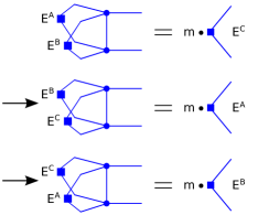
Figure 28: The self-consistent iteration process for environment matrix when the tensors do not have rotational symmetry. We introduce three different environment matrices, $E^{A}$, $E^{B}$ and $E^{C}$. One cycle of iteration consists of three steps: 1. Input $E^{A}$ and $E^{B}$ to update $E^{C}$; 2. Input $E^{B}$ and $E^{C}$ to update $E^{A}$; 3. Input $E^{C}$ and $E^{A}$ to update $E^{B}$. After iterating for enough number of steps, all three self-consistent equation will be simultaneously satisfied.

Figure 29: Expectation value of an operator with non-rotational-symmetric tensor networks. Note here that there are three different types of environment matrices.

Our method could be easily generalized to non-rotationally symmetric tensors by introducing a three-step iteration process, shown in Fig. 28. (Recall that this is different from the symmetric iteration process in Fig. 19.) In this three-step iteration process, we introduce three different environment matrices, which then iterate in a cyclic fashion. Now, any physical quantities could again be calculated by sandwiching the operator in between two layers of tensor network states, surrounded by three different types of environment matrices shown in Fig. 29, and all of our previous analysis follows. (Again compare this with Fig. 18, where there was only one type of environment matrix.)

With the above three-step iteration process, the environment matrix of our “string crystal” state could then be obtained as follows:

$$E^{A}=\begin{pmatrix}1&0\\ 0&0\end{pmatrix},\ \ E^{B}=E^{C}=\begin{pmatrix}0&0\\ 0&1\end{pmatrix}.$$ (39)

Note that the above $E^{B}$ and $E^{C}$ do not really break the $\mathbb{Z}_{2}\times\mathbb{Z}_{2}$ symmetry shown in eqn (37). This is because the iteration process for $E^{B}$ and $E^{C}$ are both linear, so an overall minus sign does not affect the iteration result. Thus $E^{B}$ and $E^{C}$ could only be determined up to a sign, which is a fictitious gauge degree of freedom and have no physical meaning. Thus $E^{B}\to-E^{B}$ does not correspond to breaking the $\mathbb{Z}_{2}\times\mathbb{Z}_{2}$ symmetry, and “string crystal” state indeed does not possess $\mathbb{Z}_{2}$ topological order.

VIII Conclusions

In this paper, we proposed a new signature for phase transitions between tensor-network states using the environment matrices. Different phases are distinctively labeled by different symmetry structures in the environment matrices. Thus through carefully studying different symmetry structures of the environment matrix, we could identify different phases and obtain the detailed phase boundaries for both symmetry-breaking transitions and topological phase transitions. This greatly helps us in identifying topological orders or SPT orders from a generic tensor-network state.

The environment matrix is obtained through a very simple iteration process using the tensor-network state, in both $1D$ and $2D$. This iteration process provides a self-consistent environment matrix that summarizes the contributions from far away sites, and is like a “mean-field” theory for tensor-networks. In the same line of thinking, the environment matrix serves like an “order parameter”. What’s special about this “mean-field” theory is that it’s suitable for studying long-range entangled states, and is thus suitable for tackling topological phase transitions.

In $1D$, we demonstrated that this new signature could be easily combined with existing numerical methods like DMRG or iTEBD to identify SPT phases. We first obtain the ground state in a matrix-product form by applying these $1D$ numerical methods. Then we calculate the environment matrix, either through direct iteration process or through a twisted iteration process (where the symmetry transformation $g$ is sandwiched in between the double tensor in the iteration process). By simply comparing the scaling factors in the two iteration process, we could identify which SPT phase we are in, thus providing an easy way to identify SPT orders directly from a matrix-product state.

In $2D$, the iteration process gives a very efficient way of calculating variational energies, which in turn leads to a simple numerical methods in obtaining gound state wave function by minimizing the energy. If we require the ground state tensors to have the proper on-site symmetry, iteration process could give us environment matrices that have drastically different symmetry structures, labeling different (topological) phases. Note that the on-site symmetry doesn’t have to be a physical symmetry— internal gauge symmetry is also valid.

The above numerical method is very general and could be easily applied to many interesting systems in higher dimension including $3D$ systems. This will open new doors in numerical study of higher dimensional systems.

This research is supported by NSF Grant No. DMR-1005541 and NSFC 11274192. XGW is also supported by the BMO Financial Group and the John Templeton Foundation Grant No. 39901. Research at Perimeter Institute is supported by the Government of Canada through Industry Canada and by the Province of Ontario through the Ministry of Research.

References

- von Klitzing et al. (1980) K. von Klitzing, G. Dorda, and M. Pepper, Phys. Rev. Lett. 45, 494 (1980).
- Tsui et al. (1982) D. C. Tsui, H. L. Stormer, and A. C. Gossard, Phys. Rev. Lett. 48, 1559 (1982).
- Kane and Mele (2005) C. L. Kane and E. J. Mele, Phys. Rev. Lett. 95, 146802 (2005), cond-mat/0506581 .
- Bernevig and Zhang (2006) B. A. Bernevig and S.-C. Zhang, Phys. Rev. Lett. 96, 106802 (2006), cond-mat/0504147 .
- Moore and Balents (2007) J. E. Moore and L. Balents, Phys. Rev. B 75, 121306 (2007), cond-mat/0607314 .
- Fu et al. (2007) L. Fu, C. L. Kane, and E. J. Mele, Phys. Rev. Lett. 98, 106803 (2007), cond-mat/0607699 .
- Kitaev (2009) A. Kitaev, in Advances in Theoretical Physics: Landau Memorial Conference, Chernogolovka, Russia, 2008, Vol. AIP Conf. Proc. No. 1134, edited by V. Lebedev and M. Feigel’man (AIP, Melville, NY, 2009) p. 22, arXiv:0901.2686 .
- Ryu et al. (2009) S. Ryu, A. Schnyder, A. Furusaki, and A. Ludwig, New J. Phys. 12, 065010 (2009), arXiv:0912.2157 .
- Wen (1989) X.-G. Wen, Phys. Rev. B 40, 7387 (1989).
- Wen and Niu (1990) X.-G. Wen and Q. Niu, Phys. Rev. B 41, 9377 (1990).
- Wen (1990) X.-G. Wen, Int. J. Mod. Phys. B 4, 239 (1990).
- Keski-Vakkuri and Wen (1993) E. Keski-Vakkuri and X.-G. Wen, Int. J. Mod. Phys. B 7, 4227 (1993).
- Levin and Wen (2005) M. A. Levin and X.-G. Wen, Phys. Rev. B 71, 045110 (2005).
- Chen et al. (2010a) X. Chen, Z.-C. Gu, and X.-G. Wen, Phys. Rev. B 82, 155138 (2010a).
- (15) F. Liu, Z. Wang, Y.-Z. You, and X.-G. Wen, arXiv:1303.0829 .
- (16) Z.-C. Gu, Z. Wang, and X.-G. Wen, arXiv:1010.1517 .
- Kong and Wen (2014) L. Kong and X.-G. Wen, (2014), arXiv:1405.5858 .
- Barkeshli et al. (2014) M. Barkeshli, P. Bonderson, M. Cheng, and Z. Wang, (2014), arXiv:1410.4540 .
- Chen et al. (2012) X. Chen, Z.-C. Gu, Z.-X. Liu, and X.-G. Wen, Science 338, 1604 (2012).
- Kapustin (2014) A. Kapustin, (2014), arXiv:1404.6659 .
- Wen (2014a) X.-G. Wen, (2014a), arXiv:1410.8477 .
- Gu and Wen (2009) Z.-C. Gu and X.-G. Wen, Phys. Rev. B 80, 155131 (2009).
- Wen (2012) X.-G. Wen, (2012), arXiv:1212.5121 .
- Zhang et al. (2012) Y. Zhang, T. Grover, A. Turner, M. Oshikawa, and A. Vishwanath, Phys. Rev. B 85, 235151 (2012), arXiv:1111.2342 .
- Cincio and Vidal (2013) L. Cincio and G. Vidal, Phys. Rev. Lett. 110, 067208 (2013), arXiv:1208.2623 .
- Zaletel et al. (2012) M. P. Zaletel, R. S. K. Mong, and F. Pollmann, (2012), arXiv:1211.3733 .
- Tu et al. (2013) H.-H. Tu, Y. Zhang, and X.-L. Qi, Phys. Rev. B 88, 195412 (2013), arXiv:1212.6951 .
- Pollmann and Turner (2012) F. Pollmann and A. M. Turner, Phys. Rev. B 86, 125441 (2012), arXiv:1204.0704 .
- Hung and Wen (2013) L.-Y. Hung and X.-G. Wen, (2013), arXiv:1311.5539 .
- Wen (2014b) X.-G. Wen, Phys. Rev. B 89, 035147 (2014b), arXiv:1301.7675 .
- Moradi and Wen (2014) H. Moradi and X.-G. Wen, (2014), arXiv:1401.0518 .
- He et al. (2014) H. He, H. Moradi, and X.-G. Wen, (2014), arXiv:1401.5557 .
- Gu et al. (2008) Z.-C. Gu, M. Levin, and X.-G. Wen, Phys. Rev. B 78, 205116 (2008).
- Vidal (2007a) G. Vidal, Phys. Rev. Lett. 98, 070201 (2007a).
- Banuls et al. (2009) M. C. Banuls, M. B. Hastings, F. Verstraete, and J. I. Cirac, Phys. Rev. Lett. 102, 240603 (2009).
- Perez-Garcia et al. (2008) D. Perez-Garcia, M. M. Wolf, M. Sanz, F. Verstraete, and J. I. Cirac, Phys. Rev. Lett. 100, 167202 (2008).
- Pollmann et al. (2010) F. Pollmann, E. Berg, A. M. Turner, and M. Oshikawa, Phys. Rev. B 81, 064439 (2010), arXiv:0910.1811 .
- Chen et al. (2011) X. Chen, Z.-C. Gu, and X.-G. Wen, Phys. Rev. B 83, 035107 (2011), arXiv:1008.3745 .
- Schuch et al. (2011) N. Schuch, D. Perez-Garcia, and I. Cirac, Phys. Rev. B 84, 165139 (2011), arXiv:1010.3732 .
- Vidal (2007b) G. Vidal, Phys. Rev. Lett. 98, 070201 (2007b), cond-mat/0605597 .
- Xiang et al. (2001) T. Xiang, J. Lou, and Z. Su, Phys. Rev. B 64, 104414 (2001).
- Legeza and Solyom (2004) O. Legeza and J. Solyom, Phys. Rev. B 70, 205118 (2004).
- Vidal et al. (2003) G. Vidal, J. I. Latorre, E. Rico, and A. Kitaev, Phys. Rev. Lett. 90, 227902 (2003).
- Srednicki (1993) M. Srednicki, Phys. Rev. Lett. 71, 666 (1993).
- Plenio et al. (2005) M. B. Plenio, J. Eisert, J. DreiBig, and M. Cramer, Phys. Rev. Lett. 94, 060503 (2005).
- Blote and Deng (2002) H. W. J. Blote and Y. Deng, Phys. Rev. E 66, 066110 (2002).
- Gu et al. (2009) Z.-C. Gu, M. Levin, B. Swingle, and X.-G. Wen, Phys. Rev. B 79, 085118 (2009).
- Trebst et al. (2007) S. Trebst, P. Werner, M. Troyer, K. Shtengel, and C. Nayak, Phys. Rev. Lett. 98, 070602 (2007).
- Chen et al. (2010b) X. Chen, B. Zeng, Z.-C. Gu, I. L. Chuang, and X.-G. Wen, Phys. Rev. B 82, 165119 (2010b).