Refining Existential Properties
in Separation Logic Analyses

Abstract

In separation logic program analyses, tractability is generally achieved by restricting invariants to a finite abstract domain. As this domain cannot vary, loss of information can cause failure even when verification is possible in the underlying logic. In this paper, we propose a CEGAR-like method for detecting spurious failures and avoiding them by refining the abstract domain. Our approach is geared towards discovering existential properties, e.g. “list contains value x”. To diagnose failures, we use abduction, a technique for inferring command preconditions. Our method works backwards from an error, identifying necessary information lost by abstraction, and refining the forward analysis to avoid the error. We define domains for several classes of existential properties, and show their effectiveness on case studies adapted from Redis, Azureus and FreeRTOS.

1 Introduction

Abstraction is often needed to automatically prove safety properties of programs, but finding the right abstraction can be difficult. Techniques based on CEGAR (CounterExample-Guided Abstraction Refinement) [11, 20] can automatically synthesise an abstraction that is sufficient for proving a given property. Particularly successful has been the application of CEGAR to predicate abstraction [15], enabling automated verification of a wide range of (primarily control-flow driven) safety properties [1, 8, 19].

Meanwhile, separation logic has emerged as a useful domain for verifying shape-based safety properties [2, 3, 7, 14, 26]. Its success stems from its ability to compositionally represent heap operations. The domain of separation logic formulae is infinite, so to ensure termination, program analyses abstract them by applying a function with a finite codomain [13]. Although this approach has proved effective in practice, it does not provide a means to recover from spurious errors caused by over-abstraction.

This paper proposes a method for automated tuning of abstractions in separation logic analyses. Instead of a single abstraction, our method works with families of abstractions parameterised by multisets, searching for a parameter that makes the analysis succeed. Expanding the multiset refines the abstraction, i.e. makes it more precise.

Our method uses a forward analysis that computes a fixpoint using the current parameterised abstraction, and a backward analysis that refines this abstraction by expanding the multiset parameter. To identify the cause of the error and propagate that information backwards along the counter-examples, we use abduction, a technique for calculating sufficient preconditions of program commands [7]. We use the difference in symbolic states generated during forward and backward analysis to select new elements to add to the multiset.

Our approach focuses on existential properties, where we need to track some elements of a data structure more precisely than the others. For example, we define the domain of “lists containing at least particular values” (where the multiset parameter specifies the values). In general, our approach works well for similar existential properties, e.g. “lists containing a particular subsequence”. Existential properties arise e.g. when verifying that key-value stores preserve values, or in structures that depend on sentinel nodes.

Our approach is complementary to standard separation logic shape analyses. It adds a new tool to the analysis toolbox, but it is not a general abstraction-refinement solution. In particular, universal properties such as “all list nodes contain a particular value” are not handled. This is a result of our analysis structure: when forward analysis fails, we look for portions of the symbolic state sufficient to avoid the fault, and seek to protect them from abstraction. This is intrinsically an existential process.

1.1 Related Work

As in Berdine et al. [4] we wish to automate the process of ‘tweaking’ shape abstractions. In [4], abstract counter-examples are passed to a SMT solver, which produces concrete counter-example traces. These traces determine so-called doomed states, conceptually the same as those singled out for refinement by our procedure. An advantage of our approach is that we use information from the failed proof to inform the abstraction refinement step, rather than exhaustively trying possible refinements as in [4]. This aside, the two approaches are largely complementary: [4] focuses on discovering shape refinements, while our work focuses on data properties.

Our approach operates lazily, but in contrast to lazy abstraction [19], we do not re-compute the abstract post operator each time we refine the abstraction. The intermediate formulae we compute during backward analysis can be seen as interpolants [22], but rather than taking these directly for refining the abstraction, we use them to select new parameters which have the effect of refining the abstraction. Such automatic discovery of parameters for parameterised domains is similar to Naik et al. [23], however, instead of analyzing concrete tests, we analyze abstract counter-examples.

Our notion of an abstraction function is similar to widening [12]. However, refining the abstraction with the least upper bound (as Gulavani and Rajamani [17]) would not converge due to the presence of recursive data structures. [9] gives a widening for shape domains, but this widening does not account for data, nor explicitly track existential properties. Refinement with an interpolated widen [16], while similar to ours, is also not applicable as we do not work in a complete lattice that is closed under Craig interpolation. Shape analyses such as TVLA [24] have been adapted for abstraction refinement  [5, 21], however, we believe these approaches could not automatically handle verification of existential properties such as those in §5.

The refinement process in our approach assumes a parameterised domain of symbolic heaps which can be refined by augmenting the multiset of parameters. Compared to predicate abstraction, where the abstract domain is constructed and refined automatically, in our approach we first have to hand-craft a parameterised domain. In part this reflects the intrinsic complexity of shape properties compared to properties verifiable by standard predicate abstraction.

Several authors have experimented with separation logic domains recording existential information about stored data, e.g. [25, 10]. Some of these domains could be formulated in our multiset-parametric approach, and vice versa. However, our work differs in that we focus on automating the process of refining the abstraction.

2 Intuitive Description of Our Approach

We now illustrate how over-abstraction can cause traditional separation-logic analyses to fail, and how our approach recovers from such failures. Our running example, given in Figure 1, is a simple instance of the pattern where a value is inserted into an pre-existing data-structure, the data-structure is further modified, and the program then assumes the continued presence of the inserted value. Our code first constructs a linked list of arbitrary length (we use ‘*’ for non-deterministic choice). It picks an arbitrary value for x, and creates a node storing this value. It extends the list with arbitrarily more nodes. Finally, it searches for the node storing x and faults if it is absent.

⬇ r = nil; while (*) { r = new Node(r,*); } x = *; r = new Node(r,x); while (*) { r = new Node(r,*); } t = r; res = 0; while(res==0 && t!=nil){ d = t->data; if (d==x) res = 1; t = t->next; } assert(res==1);

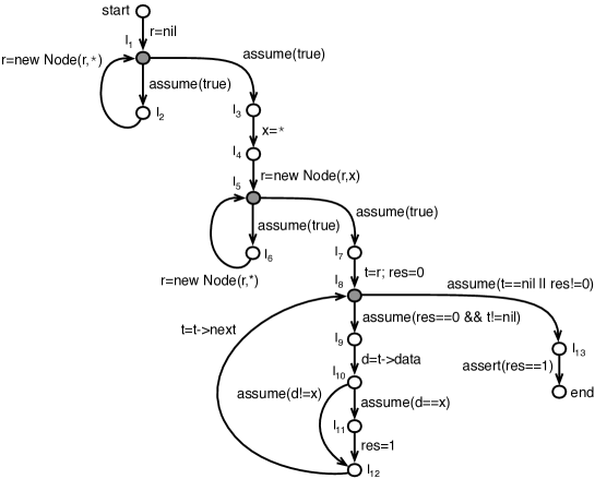
Figure 1: Left: running example. Right: associated control-flow graph. Nodes where abstraction occurs are shaded.

Suppose our abstract domain consists of the predicates $\mathsf{emp}$, representing the empty heap, $\mathsf{node}(x,y,d)$, representing a linked list node at address $x$ with next pointer $y$ and data contents $d$, and $\mathsf{list}(x,y)$, representing a non-empty list segment of unrestricted length starting at address $x$ and ending with a pointer to $y$. Nodes and list segments are related by the following recursive definition:

$$\vspace{-0.5em}\mathsf{list}(x,y)\quad\triangleq\quad\mathsf{node}(x,y,d^{\prime})\vee(\mathsf{node}(x,n^{\prime},d^{\prime})*\mathsf{list}(n^{\prime},y))$$

(Primed variables—$x^{\prime},y^{\prime}$, etc.—indicate logical variables that are existentially quantified). A traditional analysis, e.g. [13], starts with the pre-condition $\mathsf{emp}$ and propagates symbolic states over the control-flow graph (right of Fig. 1). Consider the execution of the program that adds a single node in the first while loop (node $l_{1}$) then adds $\tt x$ to the list, skips the second loop, and then searches for $\tt x$ (node $l_{8}$). Following the two list insertions (node $l_{5}$) we obtain symbolic state

$$\vspace{-0.5em}\mathsf{node}({\tt r},r^{\prime},{\tt x})\,\ast\,\mathsf{node}(r^{\prime},\mathsf{nil},d^{\prime})$$

As is typical, assume the analysis applies the following abstraction step:

$$\vspace{-0.5em}\mathsf{node}({\tt r},r^{\prime},{\tt x})\,\ast\,\mathsf{node}(r^{\prime},\mathsf{nil},d^{\prime})\;\;\leadsto\;\;\mathsf{list}({\tt r},\mathsf{nil})$$

That is, it forgets list length and data values once there are two nodes in the list. At the head of the third while-loop (node $l_{8}$) it unfolds $\mathsf{list}({\tt r},\mathsf{nil})$ back to the single-node case, yielding $\mathsf{node}({\tt r},\mathsf{nil},x^{\prime})$. Since this state is too weak to show that ${\tt x}=x^{\prime}$, the path where ${\tt res}$ is not set to $1$ appears feasible, and the analysis cannot prove assert(res==1).

Our solution.

The analysis has failed spuriously because it has abstracted away the existence of the node containing x. We cannot remove abstraction entirely, and we also cannot pick a tailored abstraction a priori, because the appropriate abstraction is sensitive to the target program and the required safety property. Instead, we work with a parameterised family of abstractions. Starting with the coarsest abstraction, we modify its parameters based on spurious failures, automatically tailoring the abstraction to the property we want to prove.

For our example, we augment the domain with a family of predicates $\mathsf{list}(\_,\_,{\{{\tt d}\}})$, representing a list where at least one node holds the value d (this domain is defined in §4). Upon failing to prove the program, our backwards analysis looks for extensions of symbolic states that would satisfy assert(res==1), and so avoid failure. Technically, this is achieved by posing successive abduction queries along the counter-example path. If an extension is found, then the difference between the formulae from forward and backward analysis identifies the cause of the spurious failure. In our example, the analysis infers that the failure was due to the abstraction of the node storing ${\tt x}$. We refine the abstraction so nodes containing ${\tt x}$ are rewritten to $\mathsf{list}(\_,\_,{\{{\tt x}\}})$, “remembering” the existence of x. This suffices to prove the program correct.

3 Analysis Structure

Symbolic heaps.

A symbolic heap $\Delta$ is a formula of the form $\Pi\,\wedge\,\Sigma$ where $\Pi$ (the pure part) and $\Sigma$ (the spatial part) are defined by:

$$\vspace{-0.5em}\Pi ::= \mathsf{true}\,\mid\mathsf{false}\,\mid\,e=e\,\mid\,e\neq e\,\mid\,p(\bar{e})\,\mid\,\Pi\,\wedge\,\Pi$$

$$\Sigma ::= \mathsf{emp}\,\mid\,s(\bar{e})\,\mid\,\Sigma\,\ast\,\Sigma$$

Here $e$ ranges over (heap-independent) expressions (built over program and logical variables), $p(\bar{e})$ over pure predicates and $s(\bar{e})$ over spatial predicates. Logical variables are (implicitly) existentially quantified; the set of all such variables in $\Delta$ is denoted by $\mathsf{EVars}(\Delta)$. $\Sigma_{1}*\Sigma_{2}$ holds if the state can be split into two parts with disjoint domains, one satisfying $\Sigma_{1}$ and the other $\Sigma_{2}$. A disjunctive symbolic heap is obtained by combining symbolic heaps (both the pure and spatial part) with disjunction. We identify a disjunctive heap with the set of its disjuncts, and also denote such heaps with $\Delta$. The set of all consistent symbolic (resp. disjunctive) heaps is denoted by $\mathsf{SH}{}$ (resp. $\mathcal{P}(\mathsf{SH}{}){}$).

Abstract domain.

Our abstract domain is the join-semilattice $(\mathcal{P}(\mathsf{SH}{})^{\top},\vdash,\sqcup,\top)$, where $\mathcal{P}(\mathsf{SH}{})^{\top}\triangleq\mathcal{P}(\mathsf{SH}{}){}\cup\{\top\}$, the partial order is given by the entailment relation $\vdash$, the join $\sqcup$ is disjunction, and the top element, $\top$, represents error.

We assume a sound theorem prover that can deal with entailments between symbolic heaps, frame inference, and abduction queries (square brackets denote the computed portion of the entailment):

• $\Delta_{1}\vdash\Delta_{2}\,\ast\,[\Delta_{F}]$ (frame inference): given $\Delta_{1}$ and $\Delta_{2}$, find the frame $\Delta_{F}$ such that $\Delta_{1}\vdash\Delta_{2}\,\ast\,\Delta_{F}$ holds;

• $\Delta_{1}\,\ast\,[\Delta_{A}]\vdash\Delta_{2}$ (abduction): given $\Delta_{1}$ and $\Delta_{2}$, find the ‘missing’ assumption $\Delta_{A}$ such that $\Delta_{1}\,\ast\,\Delta_{A}\vdash\Delta_{2}$ holds.

Specifications and programs.

We assume that each atomic command $c\in\mathsf{Cmd}{}$ is associated with a specification $\{P\}\,c\,\{Q\}$, consisting of a precondition $P$ and a postcondition $Q$ in $\mathsf{SH}{}$ (in fact, our case studies use specifications expressed by using points-to and (dis)equalities only). We define $\mathsf{assume}(e)\triangleq\{{\sf true}\}\,\{e\}$ and $\mathsf{assert}(e)\triangleq\{e\}\,\{e\}$. Specifications are interpreted using standard partial correctness: $\{P\}\,c\,\{Q\}$ holds iff when executing $c$ from a state satisfying $P$, $c$ does not fault, and if it terminates then the resulting state satisfies $Q$. As is standard in separation logic, we also assume specifications are tight: $c$ will not access any resources outside of the ones described in $P$.

We represent programs using a variant of intra-procedural control-flow graphs [19] over the set of atomic commands $\mathsf{Cmd}{}$. A CFG consists of a set of nodes $\mathsf{N}{}$ containing distinguished starting and ending nodes $\mathsf{start}{},\mathsf{end}{}\in\mathsf{N}{}$, and functions, $\mathsf{succ}\colon\mathsf{N}{}\to\mathcal{P}(\mathsf{N}{})$ and $\mathsf{cmd}\colon\mathsf{N}{}\times\mathsf{N}{}\rightharpoonup{}\mathsf{Cmd}{}$, representing node successors and edge labels. All nodes either have a single successor, or all outgoing edges are labelled with command $\mathsf{assume}(e)$ for the condition $e$ that must hold for that edge to be taken.

Forward and backward transfer.

We define the abstract forward semantics of each atomic command $c$ by a function $\llbracket c\rrbracket\colon\mathsf{SH}{}\to\mathcal{P}(\mathsf{SH}{})^{\top}$. The function $\llbracket c\rrbracket$, fusing together rearrangement (materialisation) and symbolic execution [24, 2, 13, 7], is defined using the frame rule, which allows any triple $\{P\}\,c\,\{Q\}$ to be extended by an arbitrary frame $\Delta_{F}$ that is not modified by $c$:

$$\llbracket c\rrbracket(\Delta)\quad\triangleq\quad\left\{\begin{array}[]{l@{\;\;\;}l}\top&\textrm{if }\nexists\Delta_{F}\ldotp\,\Delta\vdash P\,\ast\,\Delta_{F}\\[1.99997pt] \{Q\,\ast\,\Delta_{F}\mid\Delta\vdash P\,\ast\,\Delta_{F}\}&\textrm{otherwise.}\end{array}\right.$$

When there is no $\Delta_{F}$ such that $\Delta\vdash P\,\ast\,\Delta_{F}$, the current heap $\Delta$ does not satisfy the precondition $P$ of the command, and so execution may result in an error. We assume that the prover filters out inconsistent heaps. Lifting disjunctions to sets on the left-hand side is justified by the disjunction rule of Hoare logic. We lift $\llbracket c\rrbracket$ to a forward transfer function $\mathcal{P}(\mathsf{SH}{})^{\top}\to\mathcal{P}(\mathsf{SH}{})^{\top}$ by mapping $\top$ to $\top$ and a set of symbolic heaps to the join of their $\llbracket c\rrbracket$-images.

We use abduction to transfer symbolic heaps backwards: given a specification $\{P\}\,c\,\{Q\}$ and disjunctive symbolic heap $\Delta$, if $\Delta_{A}$ is such that $Q\,\ast\,\Delta_{A}\vdash\Delta$ then $\{P\,\ast\,\Delta_{A}\}\,c\,\{\Delta\}$, i.e., we can “push” $\Delta$ backwards over $c$ to obtain $P\,\ast\,\Delta_{A}$ as a pre-state. This gives rise to a backward transfer function $\llbracket c\rrbracket^{\leftarrow}\colon\mathcal{P}(\mathsf{SH}{}){}\to\mathcal{P}(\mathsf{SH}{}){}$ defined by:

$$\llbracket c\rrbracket^{\leftarrow}(\Delta)\quad\triangleq\quad\textit{choose}(\{P\,\ast\,\Delta_{A}\mid Q\,\ast\,\Delta_{A}\vdash\Delta\})$$

The heuristic function $\textit{choose}(-)$ selects a ‘good’ abduction solution (there can be many, e.g. a trivial one, $\mathsf{false}$). For some fragments best solutions are possible: e.g. the disjunctive points-to fragment with (dis)equalities [7], a variation of which we use in our backward analysis. Along $\mathsf{assume}$-edges we have $\llbracket\mathsf{assume}(e)\rrbracket^{\leftarrow}(\Delta)\,=\,\mathsf{wp}(\mathsf{assume}(e),\Delta)\,=\,\neg e\,\vee\,\Delta$.

3.1 Forward Analysis, Abstraction Function, and Parametricity

Forward analysis attempts to compute an inductive invariant $\mathsf{N}{}\to\mathcal{P}(\mathsf{SH}{})^{\top}$. It gradually weakens the strongest property by propagating symbolic heaps along CFG edges using the forward transfer, and joining the obtained $\llbracket c\rrbracket$-images at each CFG node. Since our abstract domain is infinite, and transfer functions are not necessarily monotone, forward propagation alone may not reach a fixpoint, or even converge towards one.

We call a pair $(\mathsf{SH}{},\mathsf{abs})$ an analysis. To ensure termination, propagated symbolic heaps are abstracted into a finite set, and the propagation process is made inflationary. Abstraction is realised by a function $\mathsf{abs}\colon\mathsf{SH}{}\to\mathsf{CSH}{}$ whose codomain is a finite subset $\mathsf{CSH}{}$ of $\mathsf{SH}{}$. At each step, $\mathsf{abs}$ replaces the propagated symbolic heap with a logically weaker one in $\mathsf{CSH}{}\cup\{\top\}$. We require $\mathsf{abs}$ to be inflationary, i.e., that it soundly over-approximates symbolic heaps with respect to $\vdash$. Making the propagation inflationary means that instead of computing the (least) fixed-point of the functional $\Phi\colon(\mathsf{N}{}\to\mathcal{P}(\mathsf{SH}{})^{\top})\to(\mathsf{N}{}\to\mathcal{P}(\mathsf{SH}{})^{\top})$, we compute the inflationary fixed-point of the functional $X\mapsto X\cup\Phi(X)$.

Definition 1 (analysis comparison)

Let $\mathsf{abs}\colon\mathsf{SH}{}\to\mathsf{CSH}{}$ and $\mathsf{abs}^{\prime}\colon\mathsf{SH}{}\to\mathsf{CSH}{}^{\prime}$ be abstraction functions. We say that $\mathsf{abs}^{\prime}$ refines $\mathsf{abs}$, written $\mathsf{abs}\preceq\mathsf{abs}^{\prime}$, if $\mathsf{CSH}{}\subseteq\mathsf{CSH}{}^{\prime}$ and for every $\Delta\in\mathsf{SH}{}$, $\mathsf{abs}^{\prime}(\Delta)\vdash\mathsf{abs}(\Delta)$. We say that $(\mathsf{SH}{},\mathsf{abs}^{\prime})$ is more precise than $(\mathsf{SH}{},\mathsf{abs})$ if $\mathsf{abs}\preceq\mathsf{abs}^{\prime}$.

In §3.2 and §4 we introduce families of analyses whose abstraction functions are parameterised by a multiset (such analyses are parametric in the sense of [23]). For any such family $(\mathsf{SH}{},\mathsf{abs}_{S})_{S\in{\mathcal{M}}}$, where ${\mathcal{M}}$ is some family of multisets and $\mathsf{abs}_{S}\colon\mathsf{SH}\to\mathsf{CSH}_{S}$, we require that if $S\subseteq S^{\prime}$ then $\mathsf{abs}_{S}\preceq\mathsf{abs}_{S^{\prime}}$.

3.2 Forward-Backward Abstraction Refinement Algorithm

We now define an intra-procedural version of our analysis formally (we believe it could be made inter-procedural without difficulty – see §6). Let $(\mathsf{SH}{},\mathsf{abs}_{S})_{S\in{\mathcal{M}}}$ be a family of analyses parameterised by a multiset. Our method for abstraction refinement starts with the analysis $(\mathsf{SH}{},\mathsf{abs}_{\emptyset})$, and iteratively refines the abstraction by adding terms to the multiset $S$. The goal is to eventually obtain $S$ such that using the analysis $(\mathsf{SH}{},\mathsf{abs}_{S})$ we can compute a sufficient inductive invariant.

Forward analysis.

1 $S:=\emptyset$;  $t_{0}:=(\mathsf{start}{},\mathsf{emp}{})$;  $k:=0$;  $E_{\mathcal{T}}=\emptyset$;  $\mathcal{T}=(\{t_{0}\},E_{\mathcal{T}},t_{0})$;

2 while $\mathsf{nodes\_at}_{\mathcal{T}}(k)\neq\emptyset$ do

3       foreach $t=(n,\Delta)\in\mathsf{nodes\_at}_{\mathcal{T}}(k)$ do

4             foreach $n^{\prime}\in\mathsf{succ}(n)$ do

5                   $\mathcal{D}^{\prime}:=\llbracket\mathsf{cmd}(n,n^{\prime})\rrbracket(\Delta)$;

6                   if $\mathcal{D}^{\prime}=\top$ then

7                         Add $(t,(n^{\prime},\top))$ to $E_{\mathcal{T}}$;

8                         $k,S:=\text{{{Refine(}}{\emph{$(n^{\prime},\top),S$}}{{)}}}$;

9                         Break to the outermost while-loop;

10                        

11                  else

12                         foreach $\Delta^{\prime}\in\mathcal{D}$ do

13                               $\Delta_{\sf abs}^{\prime}:=\mathsf{abs}_{S}(\Delta^{\prime})$;

14                               if $\Delta_{\sf abs}^{\prime}\not\sqsubseteq\mathsf{inv}_{\mathcal{T}}(n^{\prime})$ then

15                                     $\mathcal{T}_{\sf old}:=\mathcal{T}$;

16                                     Add $(t,(n^{\prime},\Delta_{\sf abs}^{\prime}))$ to $E_{\mathcal{T}}$;

17                                     $\mathsf{inv}_{\mathcal{T}}:=\mathsf{inv}_{\mathcal{T}_{\sf old}}[n^{\prime}\mapsto\mathsf{inv}_{\mathcal{T}_{\sf old}}(n^{\prime})\sqcup\Delta_{\sf abs}^{\prime}]$;

18                                    

19      $k:=k+1$;

20      

Algorithm 1 Forward analysis with abstraction refinement.

Algorithm 1 shows a forward analysis from §3.1 extended with abstraction refinement. The algorithm computes a fixpoint by constructing an abstract reachability tree (ART). An ART is a tree $\mathcal{T}=(T,E,t_{0})\in\mathsf{ART}{}$ where $T$ is the set of nodes, $E$ the set of edges and $t_{0}$ the root node. We write $E_{\mathcal{T}}$ to refer to the set of edges associated with a particular ART $\mathcal{T}$. Nodes in $T$ are of the form $(n,\Delta)\in\mathsf{N}{}\times\mathsf{SH}{}$ and represent the abstract states visited during the fixpoint computation. We use the following functions to deal with the ART: $\mathsf{parent}_{\mathcal{T}}\colon T\setminus\{t_{0}\}\to T$ returning the unique parent of a node, $\mathsf{depth}_{\mathcal{T}}\colon T\to\mathbb{N}_{0}$ returning the length of the path from $t_{0}$ to $t$, and $\mathsf{nodes\_at}_{\mathcal{T}}\colon\mathbb{N}_{0}\to\mathcal{P}(T)$ returning the set of all nodes at the given depth. For $\mathcal{T}=(T,E,t_{0})$ and $\mathcal{T^{\prime}}=(T^{\prime},E^{\prime},t_{0}^{\prime})$, we write $\mathcal{T}\subseteq\mathcal{T^{\prime}}$ to indicate that $\mathcal{T}$ is a subtree of $\mathcal{T^{\prime}}$, i.e., that $T\subseteq T^{\prime}$, and $E\subseteq E^{\prime}$, and $t_{0}=t_{0}^{\prime}$. We write $\mathsf{cmd}(n,n^{\prime})$ to represent the command labelling the edge between nodes $n$ and $n^{\prime}$ and $\mathsf{spec}(n,n^{\prime})$ for the corresponding specification.

The algorithm iteratively propagates $\llbracket\cdot\rrbracket$-images of previously-computed abstract states along CFG edges, applies abstraction if the result is consistent, and joins each newly computed state with the previously-computed states at the same node. We store the invariant computed at each step using a map $\mathsf{inv}{}\colon\mathsf{ART}{}\to(\mathsf{N}{}\to\mathcal{P}(\mathsf{SH}{})^{\top})$, reflecting the fact that the invariant at a control point can be recovered from the node labels of the ART. If we have $\mathsf{nodes\_at}(k)=\emptyset$ for the current depth $k$, then we have successfully computed an inductive invariant without reaching an error.

Suppose at some point the transfer function returns $\top$, i.e., the forward analysis fails to prove a property (e.g., a pure assertion or a memory safety pre-condition of a heap-manipulating command). This can happen due to either a true violation of the property, or a spurious error caused by losing too much information somewhere along the analysis. The algorithm then invokes Algorithm 2, Refine, to check for feasibility of the error and, if it is spurious, to refine the abstraction.

1 Refine($t^{\top}\colon T$, $S\colon{\mathcal{M}}$)$\colon N_{0}\times{\mathcal{M}}$

2 begin

3       $k:=\mathsf{depth}(t^{\top})-1$;

4       $t_{\sf curr}:=t^{\top};\;\;t_{\sf prev}:=\mathsf{parent}(t^{\top})$;

5       $\{P\}\,\_\,\{\_\}:=\mathsf{spec}(t_{\sf prev}.n,t_{\sf curr}.n)$;

6       Solve $\overline{t_{\sf prev}.\Delta}\,\ast\,[\Delta_{A}]\vdash P\,\ast\,\mathsf{true}$;

7       $\Delta_{\sf prev}^{\prime}:=\overline{t_{\sf prev}.\Delta}\,\ast\,\Delta_{A}$;

8       $\mathsf{path}_{\sf fwd}:=t_{\sf prev}.\Delta;\;\;\mathsf{path}_{\sf bwd}:=\Delta_{\sf prev}^{\prime}$;

9       while $k>0$ do

10             $t_{\sf curr}:=t_{\sf prev};\;\;t_{\sf prev}:=\mathsf{parent}(t_{\sf curr});\;\;\Delta_{\sf curr}^{\prime}:=\Delta_{\sf prev}^{\prime}$;

11             $\Delta_{\sf prev}^{\prime}:=\llbracket\mathsf{cmd}(t_{\sf prev}.n,t_{\sf curr}.n)\rrbracket^{\leftarrow}(\Delta_{\sf curr}^{\prime})$;

12             $\mathsf{path}_{\sf fwd}:=t_{\sf curr}.\Delta\cdot\mathsf{path}_{\sf fwd};\;\;\mathsf{path}_{\sf bwd}:=\Delta_{\sf curr}^{\prime}\cdot\mathsf{path}_{\sf bwd}$;

13             if $t_{\sf prev}.\Delta\vdash\Delta_{\sf prev}^{\prime}$ then

14                   $S:=S\cup\text{{{SelectSymbols(}}{\emph{$\mathsf{path}_{\sf fwd},\mathsf{path}_{\sf bwd}$}}{{)}}}$;

15                   Delete $t_{\sf curr}$-subtree of $\mathcal{T}$;

16                   return $k-1,S$;

17                  

18            $k:=k-1$;

19            

20      throw “error”;

21      

Algorithm 2 Backward analysis of counter-example by abduction.

Backward analysis.

Algorithm 2, Refine, operates by backward analysis of abstract counter-examples. Rather than using weakest preconditions as in CEGAR, Refine uses abduction to propagate formulae backwards along an abstract counter-example and check its feasibility. Once a point in the path is found where forward analysis agrees with the backward analysis, the mismatch between the symbolic heaps from forward and backward analyses is used to update the multiset $S$ that determines the abstraction.

$$\begin{array}[]{@{}c@{\;\;}c@{}}\begin{array}[]{@{}rl}t_{0}\colon&(\mathsf{start},\mathsf{emp})\\ t_{1}\colon&(l_{1},{\tt r}=\mathsf{nil})\\ t_{2}\colon&(l_{2},{\tt r}=\mathsf{nil})\\ t_{3}\colon&(l_{1},\mathsf{node}({\tt r},\mathsf{nil},\_))\\ t_{4}\colon&(l_{3},\mathsf{node}({\tt r},\mathsf{nil},\_))\\ t_{5}\colon&(l_{4},\mathsf{node}({\tt r},\mathsf{nil},\_))\\ t_{6}\colon&(l_{5},\mathsf{list}({\tt r},\mathsf{nil}))\\ t_{7}\colon&(l_{7},\mathsf{list}({\tt r},\mathsf{nil}))\\ \end{array}&\begin{array}[]{rl@{}}t_{8}\colon&(l_{8},\mathsf{list}({\tt r},\mathsf{nil})\,\wedge\,{\tt t}={\tt r}\,\wedge\,{\tt res}=0)\\ t_{9}\colon&(l_{9},\mathsf{list}({\tt r},\mathsf{nil})\,\wedge\,{\tt t}={\tt r}\,\wedge\,{\tt res}=0)\\ t_{10}\colon&(l_{10},\mathsf{node}({\tt r},\mathsf{nil},d^{\prime})\,\wedge\,{\tt t}={\tt r}\,\wedge\,{\tt res}=0\,\wedge\,{\tt d}=d^{\prime})\\ t_{11}\colon&(l_{12},\mathsf{node}({\tt r},\mathsf{nil},d^{\prime})\,\wedge\,{\tt t}={\tt r}\,\wedge\,{\tt res}=0\,\wedge\,{\tt d}=d^{\prime}\,\wedge\,{\tt d}\neq{\tt x})\\ t_{12}\colon&(l_{8},\mathsf{node}({\tt r},\mathsf{nil},d^{\prime})\,\wedge\,{\tt t}=\mathsf{nil}\,\wedge\,\hfill{\tt res}=0\,\wedge\,{\tt d}=d^{\prime}\,\wedge\,{\tt d}\neq{\tt x})\\ t_{13}\colon&(l_{13},\mathsf{node}({\tt r},\mathsf{nil},d^{\prime})\,\wedge\,{\tt t}=\mathsf{nil}\,\wedge\,{\tt res}=0)\\ t_{14}\colon&(\mathsf{end},\top)\\ \\ \end{array}\end{array}$$

Figure 2: Abstract counter-example for the running example (§2).

Definition 2

An abstract counter-example is a sequence $(n_{0},\Delta_{0})\ldots(n_{k},\Delta_{k})$ with:

• $n_{0}=\mathsf{start}{}$ and for all $0<i\leq k$, $n_{i}\in\mathsf{succ}(n_{i-1})$;

• $\Delta_{0}=\mathsf{emp}{}$, for all $0<i\leq k$, $\Delta_{i}\in\mathsf{abs}_{S}(\llbracket\mathsf{cmd}(n_{i-1},n_{i})\rrbracket(\Delta_{i-1}))$ and $\Delta_{k}=\top$.

Figure 2 shows the abstract counter-example for the error discussed in §2. This is the sequence of symbolic heaps computed by the analysis on its way to the error. This counter-example covers the case where the list contains just one node. The error results from over-abstraction, which has erased the information that this node contains the value 0 (this can be seen in the last non-error state, $t_{13}$).

Refine begins by finding a resource or pure assumption sufficient to avoid the terminal error in the counter-example. Let $(n_{0},\Delta_{0})\ldots(n_{k},\top)$ be an abstract counter-example with $\mathsf{cmd}(n_{k-1},n_{k})=\{P_{k}\}\,c_{k}\,\{Q_{k}\}$. Since $\llbracket c_{k}\rrbracket(\Delta_{k-1})=\top$, $\Delta_{k-1}$ misses some assumption required to satisfy $P_{k}$. To find this, Refine solves the following abduction query (line 2)—here $\overline{\Delta_{k-1}}$ is a rearrangement of $\Delta_{k-1}$, for example to expose particular memory cells:

$$\overline{\Delta_{k-1}}\,\ast\,[\Delta_{A}]\vdash P_{k}\,\ast\,\mathsf{true}.$$

The resulting symbolic heap $\Delta_{A}$ expresses resources or assumptions that, in combination with $\overline{\Delta_{k-1}}$, suffice to guarantee successful execution of $c_{k}$. If $\Delta_{A}$ is $\mathsf{false}$ then $\overline{\Delta_{k-1}}\,\ast\,[\Delta_{A}]$ is inconsistent; if this happens then the analysis will have to find a refinement under which $(n_{k-1},\Delta_{k-1})$ can be proved to be unreachable.

Letting $\Delta_{k-1}^{\prime}:=\overline{\Delta_{k-1}}\,\ast\,\Delta_{A}$, Refine computes a sufficient resource for the preceding state (line 2):

$$\Delta_{k-2}^{\prime}:=\llbracket\mathsf{cmd}(n_{k-2},n_{k-1})\rrbracket^{\leftarrow}(\Delta_{k-1}^{\prime}).$$

If $\Delta_{k-2}\vdash\Delta_{k-2}^{\prime}$ then in the step from $\Delta_{k-2}$ to $\Delta_{k-1}$ a loss of precision has happened, and we use the additional information in $\Delta_{k-1}^{\prime}$ to refine the abstraction (line 2). Otherwise, we continue pushing backwards, and generate $\Delta^{\prime}_{k-3}$, $\Delta^{\prime}_{k-4}$, etc.

Eventually, Refine either halts with $\Delta_{i}\vdash\Delta_{i}^{\prime}$ for some $i\geq 0$, or in the last step obtains $\Delta_{0}\not\vdash\Delta_{0}^{\prime}$. In the former case, Refine invokes the procedure SelectSymbols, passing it the forward and the backward sequence of symbolic heaps leading to the error (line 2). The symbols it generates are added to the multiset $S$, refining the abstraction. In the latter case, we did not find a point for refining the abstraction, so Refine reports a (still possibly spurious) error (line 2). Note that in this case the computed heap $\Delta_{0}^{\prime}$ is a sufficient pre-condition to avoid this particular abstract counter-example.

If Refine calls SelectSymbols to update the abstraction, it discards the current node and all its descendants from the ART (line 2). The ART below the refinement point will be recomputed in subsequent iterations using (possibly) stronger invariants.

Theorem 3.1 (Soundness)

If the algorithm terminates without throwing an error, the computed map $\mathsf{inv}_{\mathcal{T}}$ is an inductive invariant not containing $\top$.

Proof

Refinement in Alg. 1 is achieved by augmenting $S$ with new elements selected by SelectSymbols. Since $\mathsf{abs}_{S}\preceq\mathsf{abs}_{S^{\prime}}$ for $S\subseteq S^{\prime}$, this is immediately sound. ∎

Refinement heuristic.

SelectSymbols stands for some heuristic function which refines the abstraction. It takes two sequences, $\mathsf{path}_{\sf fwd}$ and $\mathsf{path}_{\sf bwd}$: the former is a path taken by the forward analysis from the $i$-th node of the counter-example to the error node (such that $\Delta_{i}\vdash\Delta_{i}^{\prime}$ in Alg. 2), while the latter is a path sufficient to avoid the error. SelectSymbols tries to identify symbols present in the error-avoiding path that have been lost in the forward, overly-abstracted path. Conceptually, SelectSymbols can be seen as a simpler analogue of the predicate discovery heuristics [1, 19] (it synthesizes only symbolic constants rather than predicates).

The heuristic in our implementation works by examining the syntactic structure of formulae $\Delta$ and $\Delta^{\prime}$ for which $\Delta\vdash\Delta^{\prime}$ has been established. The heuristic starts by identifying congruence classes of terms occurring in both formulae and building a tree of equalities between program variables in each congruence class. Our separation logic prover preserves the common syntactic parts of $\Delta$ and $\Delta^{\prime}$ by explicitly recording substitutions, ensuring we can recover a mapping between common variables occurring in both formulae. The heuristic then exhaustively traverses equalities in the congruence classes for each term of $\Delta^{\prime}$, and checks whether equalities can be used to strengthen $\Delta$ without making it inconsistent. Intuitively, because these equalities are mentioned in the calculated sufficient resource, they will likely be significant for program correctness. The variables in identified equalities are then used to strengthen the abstraction. We found this heuristic worked well in our case studies (see §5).

Running example revisited.

In §2 we saw a spurious error caused by over-abstracting values in the list. To fix this, we augmented the domain with predicates $\mathsf{list}(\_,\_,{\{{\tt d}\}})$, representing a list that has at least one node with value ${\tt d}$. We now show the refinement step in this domain. The backward analysis begins by solving the abduction query

$$(\mathsf{node}({\tt r},\mathsf{nil},d^{\prime})\,\wedge\,{\tt x}=d\,\wedge\,{\tt t}=\mathsf{nil}\,\wedge\,{\tt res}=0)\,\ast\,[\Delta^{\prime}_{13}]\;\vdash\;{\tt res}=1\,\ast\,[\_]$$

This yields $\Delta^{\prime}_{13}=\mathsf{false}$ as the only solution. The analysis then generates the following sequence of symbolic heaps (we omit some for brevity). Compare with the abstract counter example in Fig. 2; here $\Delta_{i}^{\prime}$ corresponds to node $t_{i}$):

$$\Delta_{12}^{\prime} = ({\tt t}\neq\mathsf{nil}\,\wedge\,{\tt res}=0\,\wedge\,\mathsf{true})$$

$$\Delta_{10}^{\prime} = (({\tt d}={\tt x}\,\wedge\,\mathsf{true})\,\vee\,(t^{\prime}\neq\mathsf{nil}\,\wedge\,{\tt res}=0\,\wedge\,\mathsf{node}({\tt t},t^{\prime},d^{\prime})\,\ast\,\mathsf{true}))$$

$$\Delta_{9}^{\prime} = ((\mathsf{node}({\tt t},t^{\prime},{\tt x})\,\ast\,\mathsf{true})\,\vee\,(t^{\prime}\neq\mathsf{nil}\,\wedge\,{\tt res}=0\,\wedge\,\mathsf{node}({\tt t},t^{\prime},d^{\prime})\,\ast\,\mathsf{true}))$$

$$\Delta_{8}^{\prime} = ((({\tt res}\neq 0\,\vee\,{\tt t}=\mathsf{nil})\,\wedge\,\mathsf{true})\,\vee\,(\mathsf{node}({\tt t},t^{\prime},{\tt x})\,\ast\,\mathsf{true})\,\vee\,$$

$$(t^{\prime}\neq\mathsf{nil}\,\wedge\,{\tt res}=0\,\wedge\,\mathsf{node}({\tt t},t^{\prime},d^{\prime})\,\ast\,\mathsf{true}))$$

$$\Delta_{7}^{\prime} = (({\tt r}=\mathsf{nil}\,\wedge\,\mathsf{true})\,\vee\,(\mathsf{node}({\tt r},t^{\prime},{\tt x})\,\ast\,\mathsf{true})\,\vee\,(t^{\prime}\neq\mathsf{nil}\,\wedge\,\mathsf{node}({\tt r},t^{\prime},d^{\prime})\,\ast\,\mathsf{true}))$$

$$\Delta_{5}^{\prime} = ({\tt r}=t^{\prime}\,\wedge\,\mathsf{true})$$

The algorithm stops at $\Delta_{5}^{\prime}$, since $\Delta_{5}\vdash\Delta_{5}^{\prime}$, and calls SelectSymbols to augment the abstraction. Our implementation looks for equalities in each $\Delta^{\prime}$ that can be used to strengthen $\Delta$. In this case, in $\Delta_{10}^{\prime}$ the heuristic identifies ${\tt d}={\tt x}$ to strengthen the corresponding $\Delta_{10}=\mathsf{node}({\tt r},\mathsf{nil},d^{\prime})\,\wedge\,{\tt t}={\tt r}\,\wedge\,{\tt res}=0\,\wedge\,{\tt d}=d^{\prime}$. Thus the heuristic selects the variable ${\tt x}$ to augment the abstraction’s multiset.

In the unrefined analysis, any predicate $\mathsf{list}(\_,\_,S)$ will be abstracted to $\mathsf{list}(\_,\_,\emptyset)$ (equivalent to $\mathsf{list}(\_,\_)$). Adding x to the multiset means that predicates of the form $\mathsf{list}(\_,\_,\{{\tt x}\})$ will be protected from abstraction. We restart the forward analysis from $t_{5}$. This time the error is avoided, and we obtain the following abstract states:

$$t_{6}^{\prime} = (l_{5},\mathsf{list}({\tt r},\mathsf{nil},\{{\tt x}\}))\ \ldots$$

$$t_{9}^{\prime} = (l_{9},\mathsf{list}({\tt r},\mathsf{nil},\{{\tt x}\})\,\wedge\,{\tt t}={\tt r}\,\wedge\,{\tt res}=0)$$

Executing from $l_{9}$ to $l_{10}$ gives two possible post-states: $\mathsf{node}({\tt r},r^{\prime},d^{\prime})\,\ast\,\mathsf{list}(r^{\prime},\mathsf{nil},\{{\tt x}\})\,\wedge\,{\tt t}={\tt r}\,\wedge\,{\tt res}=0\,\wedge\,{\tt d}=d^{\prime}$ and $\mathsf{node}({\tt r},r^{\prime},{\tt x})\,\ast\,\mathsf{list}(r^{\prime},\mathsf{nil},\emptyset)\,\wedge\,{\tt t}={\tt r}\,\wedge\,{\tt res}=0\,\wedge\,{\tt d}={\tt x}$. In fact, this refined abstraction suffices to prove the absence of errors on all paths, which completes the analysis. (Other examples may need multiple refinements)

4 Example Multiset-Parametric Analyses

We describe in detail linked lists with value refinement and sketch two other multiset families: linked lists with address refinement, and sorted linked lists with value refinement. Details for the latter two can be found in Appendix 0.B. All three families are experimentally evaluated in §5.

Linked lists with value refinement is domain used in our running example (§2). List segments are instrumented with a multiset representing the lower bound on the frequency of each variable or constant. The abstraction function is parameterised by a multiset controlling which symbols are abstracted. By expanding the multiset, the preserved frequency bounds are increased, and so the abstraction is refined.

The domain $\mathsf{SH}^{\sf mls}$ contains spatial predicates $\mathsf{node}(\cdot,\cdot,\{d\})$ and $\mathsf{list}(\cdot,\cdot,S)$ for all $S$ and $d\in S$. Here $x,y$ are locations, $d$ is a data value, $S$ is a multiset:

• $\mathsf{node}(x,y,\{d\})$ holds if $x$ points to a node whose next field contains $y$ and data field contains $d$, i.e., $\mathsf{node}(x,y,\{d\})\,\triangleq\,x\mapsto\{{\sf next}\colon y,{\sf data}\colon d\}$.

• $\mathsf{list}(x,y,S)$ holds if $x$ points to the first node of a non-empty list segment that ends with $y$, and for each value $d\in{\rm dom}(S)$, there are at least $S(d)$ nodes that store $d$.

The recursive definition of $\mathsf{list}$ in $\mathsf{SH}^{\sf mls}$ is shown in Fig. 3. We use these equivalences as folding and unfolding rules when solving entailment queries in $\mathsf{SH}^{\sf mls}$.

case $S=\emptyset$:	$\mathsf{list}(e,f,\emptyset)\;\triangleq\;$	$\mathsf{node}(e,f,\_)\,\vee\,(\mathsf{node}(e,x^{\prime},\_)\,\ast\,\mathsf{list}(x^{\prime},f,\emptyset))$
case $S=\{d\}$:	$\mathsf{list}(e,f,\{d\})\;\triangleq\;$	$\mathsf{node}(e,f,\{d\})\,\vee\,(\mathsf{node}(e,x^{\prime},\{d\})\,\ast\,\mathsf{list}(x^{\prime},f,\emptyset))$
		$\,\vee\,(\mathsf{node}(e,x^{\prime},\_)\,\ast\,\mathsf{list}(x^{\prime},f,\{d\}))$
case $|S|>1,d\in S$:	$\mathsf{list}(e,f,S)\;\triangleq\;$	$\mathsf{node}(e,x^{\prime},\{d\})\,\ast\,\mathsf{list}(x^{\prime},f,S\setminus\{d\})\,\vee\,$
		$\mathsf{node}(e,x^{\prime},\_)\,\ast\,\mathsf{list}(x^{\prime},f,S)$

Figure 3: Recursive definition of the $\mathsf{list}$ predicate in domain $\mathsf{SH}^{\sf mls}$.

$$\begin{array}[]{r@{\;\;}c@{\;\;}l}\Delta\,\wedge\,x^{\prime}=e&\rightsquigarrow_{T}^{\sf mls}&\Delta[e/x^{\prime}]\\[6.99997pt] \Delta\,\ast\,\sigma(x^{\prime},e,\_)&\rightsquigarrow_{T}^{\sf mls}&\Delta\,\ast\,\mathsf{true}\hfill\textrm{if }x^{\prime}\notin\mathsf{EVars}(\Delta)\\[6.99997pt] \Delta\,\ast\,\sigma_{1}(x^{\prime},y^{\prime},\_)\,\ast\,\sigma_{2}(y^{\prime},x^{\prime},\_)&\rightsquigarrow_{T}^{\sf mls}&\Delta\,\ast\,\mathsf{true}\hfill\textrm{if }x^{\prime},y^{\prime}\notin\mathsf{EVars}(\Delta)\\[6.99997pt] \Delta\,\ast\,\sigma_{1}(e_{1},x^{\prime},S_{1})\,\ast\,\sigma_{2}(x^{\prime},e_{2},S_{2})&\rightsquigarrow_{T}^{\sf mls}&\Delta\,\ast\,\mathsf{list}(e_{1},\mathsf{nil},\mathsf{pr}_{T}(S_{1}\cup S_{2},\Pi))\\[1.99997pt] &&\hfill\textrm{if }x^{\prime}\notin\mathsf{EVars}(\Delta,e_{1},e_{2})\wedge\Delta\vdash e_{2}=\mathsf{nil}\\[6.99997pt] \left(\begin{array}[]{@{}l@{}}\Delta\,\ast\,\sigma_{1}(e_{1},x^{\prime},S_{1})\,\ast\\ \sigma_{2}(x^{\prime},e_{2},S_{2})\,\ast\,\sigma_{3}(e_{3},f,S_{3})\end{array}\right)&\rightsquigarrow_{T}^{\sf mls}&\left(\begin{array}[]{@{}r@{}}\mathsf{list}(e_{1},e_{2},\mathsf{pr}_{T}(S_{1}\cup S_{2},\Pi))\\ \,\ast\,\Delta\,\ast\,\sigma_{3}(e_{3},f,S_{3})\end{array}\right)\\[8.99994pt] &\lx@intercol\hfil\;\;\;\textrm{if }x^{\prime}\notin\mathsf{EVars}(\Delta,e_{1},e_{2},e_{3},f)\wedge\Delta\vdash e_{2}=e_{3}\lx@intercol\\[6.99997pt] \Delta\,\ast\,\mathsf{list}(e,f,S)&\rightsquigarrow_{T}^{\sf mls}&\mathsf{list}(e,f,\mathsf{pr}_{T}(S,\Pi))\end{array}$$

Figure 4: Abstract reduction system $\rightsquigarrow_{T}^{\sf mls}$ defining the abstraction function $\mathsf{abs}_{T}^{\sf mls}$. (In the rules, $\sigma,\sigma_{i}$ range over $\{\mathsf{node},\mathsf{list}\}$. The pure assumption $\Pi$ is supplied by the analysis.)

Abstraction.

Let $T$ be a finite multiset of program variables and constants. In Fig. 4, we define a parametric reduction system $\rightsquigarrow_{T}^{\sf mls}$, which rewrites symbolic heaps from $\mathsf{SH}^{\sf mls}$ to canonical heaps whose data and multiset values are congruent to elements of $T$. Except for the final rule, the relation $\rightsquigarrow_{T}^{\sf mls}$ resembles the abstraction for plain linked lists developed by Distefano et al. [13, table 2].

The final reduction rule replaces every predicate $\mathsf{list}(e,f,S)$ with the bounded predicate $\mathsf{list}(e,f,\mathsf{pr}_{T}(S,\Pi))$. The operator $\mathsf{pr}_{T}$ extracts the maximal subset of $S$ such that no element appears more frequently than it does in $T$ (modulo given pure assumptions $\Pi$). Let $\sim_{\Pi}$ be the equivalence relation $x\sim_{\Pi}y\triangleq\Pi\vdash x=y$. Fix a representative for each equivalence class of $\sim_{\Pi}$, and for a multiset $S$, denote by $S/_{\Pi}$ the multiset of $\sim_{\Pi}$-representatives where the multiplicity of a representative $x$ is $\sum_{x\sim_{\Pi}y}S(y)$. Writing $x\cdot n$ for a multiset element $x$ occurring with multiplicity $n$, we define $\mathsf{pr}_{T}$ by

$$\mathsf{pr}_{T}(S,\Pi)\;\triangleq\ \{x\cdot n\mid x\cdot k^{\prime}\in S/_{\Pi}\,\wedge\,\exists d^{\prime}\cdot m^{\prime}\in T/_{\Pi}\ldotp\Pi\vdash x=d^{\prime}\,\wedge\,n=\min(k^{\prime},m^{\prime})\}.$$

As $\rightsquigarrow_{T}^{\sf mls}$ has no infinite reduction sequences, it gives rise to an abstraction function $\mathsf{abs}_{T}^{\sf mls}$ by exhaustively applying the rules until none apply.

Lemma 1 (Finiteness)

If $T$ is finite and there are only finitely many program variables then the domain $\mathsf{CSH}_{T}^{\sf mls}\triangleq\{\Delta\mid\Delta\not\vdash\mathsf{false}\,\wedge\,\Delta\not\rightsquigarrow_{T}^{\sf mls}\}$ is finite.

Lemma 2 (Soundness)

As $\Delta\rightsquigarrow_{T}^{\sf mls}\Delta^{\prime}$ implies $\Delta\vdash\Delta^{\prime}$, $\mathsf{abs}_{T}^{\sf mls}\colon\mathsf{SH}\to\mathsf{CSH}_{T}^{\sf mls}$ is a sound abstraction function.

Lemma 3 (Monotonicity)

If $T_{1}\subseteq T_{2}$ then $\mathsf{abs}_{T_{1}}^{\sf mls}\preceq\mathsf{abs}_{T_{2}}^{\sf mls}$.

4.1 Linked Lists with Address Refinement

⬇

int remove(Node x) {

... // (border cases)

p = hd; c = p->next;

while (c!=nil) {

if (c==x) {

p->next = c->next;

return 1;

}

p = c; c = p->next;

}

return 0;

}

Rather than preserving certain values in the list, we might need to preserve nodes at particular addresses. For example, to remove a node from a linked list we might use the procedure shown on the right. Given pre-condition $\mathsf{list}({\tt r},{\tt x})\,\ast\,\mathsf{node}({\tt x},n^{\prime},\_)\,\ast\,\mathsf{list}(n^{\prime},\mathsf{nil})$ the procedure will return 1. However, the standard list abstraction will forget the existence of the node pointed to by x, making this impossible to prove.

To preserve information of this kind, we combine the domain of linked lists, $\mathsf{SH}^{\sf rls}$, with a multiset refinement that preserves particular addresses. Because node addresses are unique, the domain contains just $\mathsf{list}$ and $\mathsf{node}$ predicates, rather than predicates instrumented with multisets. The reduction system $\rightsquigarrow_{T}^{\sf rls}$ protects addresses in the multiset $T$ from abstraction. As before, refinement consists of adding new addresses to the multiset.

4.2 Sorted Linked Lists with Value Refinement

We can apply the idea of value refinement to different basic domains, allowing us to deal with examples where different data-structure invariants are needed. In our third analysis family, we refine on the existence of particular values in a sorted list interval, rather than a simple segment. The domain $\mathsf{SH}^{\sf sls}$ contains the predicate $\mathsf{list}_{\leq}$, parameterised by an interval of the form $[\alpha,\beta\rangle$, which stores the bounds of the values in the list, and a multiset $S$, which bounds on the frequency of particular values in the interval. The abstraction function $\rightsquigarrow_{T}^{\sf sls}$ works in a similar way to $\mathsf{SH}^{\sf mls}$: the operator $\mathsf{pr}_{T}$ caps the frequency set $S$, limiting the number of values that are preserved by abstraction.

5 Experimental Evaluation

We implemented Algorithm 1 and abstract domains $\mathsf{SH}^{\sf mls}$, $\mathsf{SH}^{\sf rls}$ and $\mathsf{SH}^{\sf sls}$ in the separation logic tool ${\sf coreStar}$ [6]. Aside from superficial tweaks, we used an identical algorithm and SelectSymbols heuristic for all of our case studies. We used client-oriented specifications [18] describing datastructures from Redis (a key-value store), Azureus (a BitTorrent client) and FreeRTOS (real time operating system). Table 1 shows results.

No	Benchmark	Result	Dom	$|T|$	#Refn	$|$ART$|$	#Quer
Set
1	${\sf add}(x)$–$\ast$–${\sf mem}(x)$	$\checkmark$	$\mathsf{SH}^{\sf mls}$	1	1	83	162
2	$\ast$–${\sf add}(x)$–$\ast_{\neg{\sf del}}$–${\sf mem}(x)$	$\checkmark$	$\mathsf{SH}^{\sf mls}$	1	1	104	193
3	$\ast_{\neg{\sf del}}$–${\sf mem}(x)$–$\ast_{\neg x}$–${\sf mem}(x)$	$\checkmark$	$\mathsf{SH}^{\sf mls}$	1	1	165	280
4	$\ast_{{\sf add}(x)}$–${\sf all\_equal\_to\_}x$	$\infty$	$\mathsf{SH}^{\sf mls}$
5	$\ast_{{\sf add}(x)}$–${\sf all\_sorted}$	$\top$	$\mathsf{SH}^{\sf mls}$
Multiset
6	${\sf add}(x)$–${\sf add}(x)$–${\sf del}(x)$–${\sf mem}(x)$	$\checkmark$	$\mathsf{SH}^{\sf mls}$	2	1	67	91
7	$\ast$–${\sf add}(x)$–$\ast_{\neg{\sf del}}$–${\sf mem}(x)$	$\checkmark$	$\mathsf{SH}^{\sf mls}$	1	1	112	205
8	$\ast_{\neg{\sf del}}$–${\sf mem}(x)$–$\ast_{\neg x}$–${\sf mem}(x)$	$\checkmark$	$\mathsf{SH}^{\sf mls}$	1	1	171	312
9	$\ast$–${\sf add}(x)$–$\ast_{\neg{\sf del}}$–${\sf add}(x)$–$\ast_{\neg{\sf del}}$–${\sf del}(x)$–${\sf mem}(x)$	$\checkmark$	$\mathsf{SH}^{\sf mls}$	2	2	219	458
Map
10	$\ast$–${\sf put}(k,v)$–$\ast_{\neg k}$–${\sf get}(k)$	$\checkmark$	$\mathsf{SH}^{\sf mls}$	1	1	118	215
11	$\ast$–${\sf rem}(k)$–${\sf bound}(k)$	$\checkmark$	$\mathsf{SH}^{\sf mls}$	1	1	92	168
ByteBufferPool
12	Property 1	$\checkmark$	$\mathsf{SH}^{\sf rls}$	1	1	154	231
13	Property 2	$\checkmark$	$\mathsf{SH}^{\sf rls}$	2 (1)	1	189	270
14	Property 3	$\checkmark$	$\mathsf{SH}^{\sf rls}$	6 (2)	4	316	511
FreeRTOS list
15	Property 4	$\checkmark$	$\mathsf{SH}^{\sf mls}$	1	1	91	158
16	Property 5	$\checkmark$	$\mathsf{SH}^{\sf sls}$	6	5	425	971

Table 1: Experimental Results. Benchmarks verified by the analysis are marked with $\checkmark$, those where it threw an error with $\top$ and those where it did not terminate with $\infty$. Dom is the domain used for the analysis, $|T|$ is the size of the multiset $T$ after the final refinement (number in parentheses denotes the size of the minimal sufficient $T$), #Refn is the no. of refinement steps, $|$ART$|$ the no. symbolic states in the final ART, and #Quer the no. queries sent to the prover.

Set, Multiset and Map. These are synthetic benchmarks based on specifications for Redis [18]. They check various aspects of functional correctness—for example, that following deletion a key is no longer bound in the store. Furthermore, we check these specifications across dynamic updates which may modify the data structures involved—for example, by removing duplicate bindings to optimize for space usage.

The Set and Multiset benchmarks apply operations ${\sf add}$ (add an element), ${\sf del}$ (delete an element) and ${\sf mem}$ (test for membership) to a list-based set (multiset, respectively) in the order indicated by the benchmark name. The symbols $\ast$, $\ast_{\neg{\sf del}}$ and $\ast_{\neg x}$ respectively denote applying all operations any number of times with any argument, all operations except ${\sf del}$, and all operations but excluding $x$ as an argument. For Map benchmarks the operations ${\sf put}$ (insert a key-value pair), ${\sf get}$ (retrieve a value for the given key), ${\sf rem}$ (remove a key with the associated value) and ${\sf bound}$ (check if the key is bound) are to a list-based map. For benchmarks 1,2,6,7,9,10 the goal was to prove that the last operation returns ${\sf true}$; for benchmark 11 that it returns ${\sf false}$; and, for benchmarks 3 and 8 that the two ${\sf mem}$ operations return the same value. Benchmark 4 illustrates a universal property that causes our analysis in $\mathsf{SH}^{\sf mls}$ to loop forever by adding $x$ to $T$ at each refinement step. Benchmark 5 is a universal property for which our analysis in $\mathsf{SH}^{\sf mls}$ fails to find an inductive invariant due to the ordering predicate (using $\mathsf{SH}^{\sf sls}$ on the same benchmark loops forever).

ByteBufferPool. Azureus uses a pool of ByteBuffer objects to store results of network transfers. In early versions, free buffers in this pool were identified by setting the buffer position to a sentinel value. The ByteBufferPool benchmarks check properties of this pool. Property 1 checks that if the pool is full and a buffer is freed, that just-freed buffer is returned the next time a buffer is requested. Property 2 checks that if the pool has some number of free buffers, then no new buffers are allocated when a buffer is requested. Property 3 checks that if the pool has at least two free buffers, then two buffer requests can be serviced without allocating new buffers.

FreeRTOS list. This is a sorted cyclic list with a sentinel node, used task management in the scheduler. The value of the sentinel marks the end of the list—for instance, on task insertion the list is traversed to find the right insertion point and the guard for that iteration is the sentinel value. To check correctness of the shape after insertion (Property 4) it suffices to remember that the sentinel value is in the list. To check that tasks are also correctly sorted according to priorities (Property 5) we need to keep track of list sortedness and all possible priorities as splitting points.

6 Conclusions and Limitations

We have presented a CEGAR-like abstraction refinement scheme for separation logic analyses, aimed at refining existential properties of programs, in which we want to track some elements of a data structure more precisely than others.

Our prototype tool is built on ${\sf coreStar}$ [6], and we expect our approach would combine well with other separation logic tools, e.g. [7, 3]. In particular, abduction is known to work well in an inter-procedural setting [7] and we thus believe our approach could be made inter-procedural without substantial further research.

Minimizing incompleteness is more challenging, as without further assumptions Algorithm 1 might diverge, or fail to recognize a spurious counter-example as infeasible. If the forward transfer function is exact (i.e., returns the strongest post-condition) and the backward transfer function is precise (i.e., for any $c$ and $\Delta$, $\llbracket c\rrbracket(\llbracket c\rrbracket^{\leftarrow}(\Delta))\vdash\Delta$) then the algorithm makes progress relative to the refinement heuristic. Intuitively, if SelectSymbols always picks a symbol such that the refined abstraction rules out the spurious counter-example, then that counter-example will never reappear in subsequent iterations. However, we are skeptical that our current heuristic satisfies this condition. For a more formal discussion, see Appendix 0.A.

Note that Berdine et al. [4] similarly do not establish progress for their analysis. Predicate abstraction techniques that do not a priori fix the set of predicates have the same issue, as do interpolation-based procedures that do not constrain the language of acceptable interpolants. In both cases, the restrictions that ensure termination also limit the set of programs that can be proved correct.

Appendix 0.A Relative Progress and Completeness

Without further assumptions, the abstraction refinement algorithm might diverge, or report a spurious counter-example which is in fact not feasible. The following idealised assumptions suffice to ensure progress and completeness (we are skeptical that condition (c) holds for our current realisation of the analysis—see below).

• The forward transfer function is exact (i.e., $\llbracket\cdot\rrbracket$-image is the strongest post-condition in the given abstract domain).

• The backward transfer function is precise (so we are able to identify spurious counter-examples). Formally, for any $c$ and $\Delta$, we have $\llbracket c\rrbracket(\llbracket c\rrbracket^{\leftarrow}(\Delta))\vdash\Delta$.

• When called with a $(\mathsf{path}_{\sf fwd},\mathsf{path}_{\sf bwd})$-pair of the counter-example and the path sufficient to avoid the error, the procedure call SelectSymbols($\mathsf{path}_{\sf fwd},\mathsf{path}_{\sf bwd}$) picks symbols $A$ for augmenting $S$ such that the spurious counter-example ending with $\mathsf{path}_{\sf fwd}$ is eliminated by the abstraction $\mathsf{abs}_{S\cup A}$.

Alg. 1 then makes progress by ensuring that a counter-example, once eliminated, remains eliminated in all subsequent iterations.

Theorem 0.A.1 (Relative progress)

Let $\gamma_{j}$ be the counter-example processed in the $j$-th refinement step. Then for all $j\geq 1$, $|\gamma_{j}|\leq|\gamma_{j+1}|$, where $|\cdot|$ denotes the length of the counter-example. In addition, if $\gamma_{j}$ is processed with value $k$ in the while-loop on line 1 of Alg. 1 then the program being analysed has no counter-examples of length less than $k$.

Proof

Let $S(j)$ denote the multiset from the $j$-th iteration of Refine. Since $\mathsf{abs}_{S(j)}\preceq\mathsf{abs}_{S(j+1)}$, no new counter-examples can appear in the part of the ART that is recomputed in the $(j+1)$-th step (invariants computed in $\mathsf{CSH}_{S(j+1)}$ will be at least as strong as those in $\mathsf{CSH}_{S(j)}$). Since (c) guarantees that the previous counter-example has been eliminated, if a new counter-example is found then the corresponding value of $k$ in the while-loop will be either the same as in the $j$-th step or larger. ∎

Theorem 0.A.2 (Relative completeness)

If the safety property is implied by an inductive invariant expressible in $\mathsf{CSH}_{S}$ for some finite multiset $S$ and assuming that those elements would eventually be selected from counter-examples by SelectSymbols then Alg. 1 terminates without throwing an error.

Proof

Since Alg. 1 proceeds in a breadth-first fashion and counter-examples to safety properties are finite, all counter-examples leading to picking elements of $S$ will eventually be processed, enabling Alg. 1 to compute an invariant in $\mathsf{CSH}_{S^{\prime}}$ for some $S^{\prime}\supseteq S$. ∎

Assumptions (a) and (b) can be satisfied (although for implementation efficiency we may choose not to). Assumption (c) is more problematic.

Forward transfer.

Without exactness, a spurious counter-example may never be eliminated, because our analysis refines only the abstraction function. Since separation logic analyses effectively calculate strongest post-conditions, we in fact have exact forward transfer, meaning spurious counter-examples can always be eliminated.

Backward transfer.

In our analysis abduction is performed on finite unfoldings of predicates, modulo an arbitrary frame, fixed along the counter-example. As a result, counter-examples are always expressed as data-structures of a particular size (rather than e.g. general lists which could be of any size). This means that counter-examples can be expressed in the points-to fragment of separation logic, in which optimal solutions are possible [7]. Thus in principle we can satisfy (b) and make backward transfer precise. However, such a complete abductive inference is of exponential complexity since it has to consider all aliasing possibilities. In our implementation, we use a polynomial heuristic algorithm (similar to [7]) which may miss some solutions, but in practice has roughly the same cost as frame inference.

Selecting symbols.

Due to its heuristic nature, it is unlikely that our implementation of SelectSymbols satisfies assumption (c). Furthermore, we are unsure whether it is generally possible to construct SelectSymbols that would satisfy (c) for an arbitrary parametric domain. While at least in principle we could employ a trivial heuristic which enumerates all multisets of symbols, that would be impractical. The problem of picking symbols which are certain to eliminate a particular counter-example seems uncomfortably close to selecting predicates for predicate abstraction sufficient to prove a given property. Many effective heuristics used in this area are incomplete (in that they may fail to find an adequate set of predicates when one exists), and there has been only a limited progress in characterising complete methods. Unfortunately, all such complete predicate refinement methods rely on interpolation, a luxury which we do not (yet) have in separation logic. More work is needed to understand the intrinsic complexity of ways for doing refinement in separation logic analyses such as the one proposed in this paper in relation to the logical properties of separation logic domains.

Appendix 0.B Details of Other Multiset-Parametric Domains

Here we give detailed definitions of the two analysis families that we sketched in §4.

0.B.1 Linked Lists with Address Refinement

This analysis allows refinement on protecting particular addresses, rather than values. We work with the domain of linked lists, which we denote $\mathsf{SH}^{\sf rls}$, built from plain spatial predicates $\mathsf{node}$ and $\mathsf{list}$.

$$\begin{array}[]{r@{\;\;}c@{\;\;}l}\Delta\,\ast\,\sigma_{1}(e_{1},x^{\prime})\,\ast\,\sigma_{2}(x^{\prime},e_{2})&\rightsquigarrow_{T}^{\sf rls}&\Delta\,\ast\,\mathsf{list}(e_{1},\mathsf{nil})\\[1.99997pt] \lx@intercol\hfil\;\;\;\;\;\;\;\;\;\;\;\;\;\;\;\;\;\;\;\;\;\;\;\;\;\;\;\;\;\;\textrm{if }x^{\prime}\notin\mathsf{EVars}(\Delta,e_{1},e_{2})\wedge\Delta\vdash e_{2}=\mathsf{nil}\wedge\forall t\in T\,.\,\Delta\nvdash e_{1}=t\lx@intercol\\[6.99997pt] \Delta\,\ast\,\sigma_{1}(e_{1},x^{\prime})\,\ast\,\sigma_{2}(x^{\prime},e_{2})\,\ast\,\sigma_{3}(e_{3},f)&\rightsquigarrow_{T}^{\sf rls}&\Delta\,\ast\,\mathsf{list}(e_{1},e_{2})\,\ast\,\sigma_{3}(e_{3},f)\\[1.99997pt] \lx@intercol\hfil\;\;\;\;\;\;\;\;\;\;\;\;\;\;\;\;\;\;\;\;\;\;\;\;\;\;\;\;\;\;\textrm{if }x^{\prime}\notin\mathsf{EVars}(\Delta,e_{1},e_{2},e_{3},f)\wedge\Delta\vdash e_{2}=e_{3}\wedge\forall t\in T\,.\,\Delta\nvdash e_{1}=t\lx@intercol\end{array}$$

Figure 5: Abstract reduction system $\rightsquigarrow_{T}^{\sf rls}$ defining the abstraction function $\mathsf{abs}_{T}^{\sf rls}$. First three rules (not shown) are the same as in Fig. 4. In the shown rules, $\sigma,\sigma_{i}$ range over $\{\mathsf{node},\mathsf{list}\}$ and the data field is elided.

Our abstraction works similarly to the abstraction for plain linked lists [13] except that it can be refined to preserve nodes at particular addresses. Fig. 5 shows rewrite rules realising the abstraction $\mathsf{abs}_{T}^{\sf rls}$. The rules are guarded by a finite set of terms $T$ representing locations—each rule is enabled only if the spatial object triggering the rule is not among the locations in $T$.

Lemma 4

$\mathsf{CSH}_{T}^{\sf rls}\triangleq\{\Delta\mid\Delta\not\vdash\mathsf{false}\,\wedge\,\Delta\not\rightsquigarrow_{T}^{\sf rls}\}$ is finite and $\mathsf{abs}_{T}^{\sf rls}\colon\mathsf{SH}\to\mathsf{CSH}_{T}^{\sf rls}$ is a sound abstraction.

Lemma 5

If $T_{1}\subseteq T_{2}$ then $\mathsf{abs}_{T_{1}}^{\sf rls}\preceq\mathsf{abs}_{T_{2}}^{\sf rls}$.

0.B.2 Sorted Linked Lists with Value Refinement

Lastly, we present an analysis that works in the domain of sorted linked lists. Our abstraction can be refined to preserve particular values in the list, as with the analysis described in §4. However, the domain consists of ordered lists segments.

$S=\emptyset$:
$\mathsf{list}_{\leq}(e,f,[\alpha,\beta\rangle,\emptyset)\;\triangleq\;$	$\alpha\leq d^{\prime}<\beta\,\wedge\,(\mathsf{node}(e,f,\{d^{\prime}\})\,\vee\,$
	$\mathsf{node}(e,x^{\prime},d^{\prime})\,\ast\,\mathsf{list}_{\leq}(x^{\prime},f,[d^{\prime},\beta\rangle,\emptyset))$
$S=\{d\}$:
$\mathsf{list}_{\leq}(e,f,[\alpha,\beta\rangle,\{d\})\;\triangleq\;$	$\mathsf{node}(e,f,\{d\})\,\vee\,$
	$d=\alpha\,\wedge\,\mathsf{node}(e,x^{\prime},\{d\})\,\ast\,\mathsf{list}_{\leq}(x^{\prime},f,[d,\beta\rangle,\emptyset)\,\vee\,$
	$d\neq\alpha\,\wedge\,\alpha\leq d^{\prime}<\beta\,\wedge\,\mathsf{node}(e,x^{\prime},d^{\prime})\,\ast\,\mathsf{list}_{\leq}(x^{\prime},f,[d^{\prime},\beta\rangle,\{d\})$
$|S|>1,d\in S$:
$\mathsf{list}_{\leq}(e,f,[\alpha,\beta\rangle,S)\;\triangleq\;$	$d=\alpha\,\wedge\,\mathsf{node}(e,x^{\prime},\{d\})\,\ast\,\mathsf{list}_{\leq}(x^{\prime},f,[d,\beta\rangle,S\setminus\{d\})\,\vee\,$
	$d\neq\alpha\,\wedge\,\alpha\leq d^{\prime}<\beta\,\wedge\,\mathsf{node}(e,x^{\prime},d^{\prime})\,\ast\,\mathsf{list}_{\leq}(x^{\prime},f,[d^{\prime},\beta\rangle,S)$

Figure 6: Recursive definition of the $\mathsf{list}_{\leq}$ predicate in domain $\mathsf{SH}^{\sf sls}$.

Domain.

The predicate $\mathsf{list}_{\leq}(x,y,[\alpha,\beta\rangle,S)$ holds if $x$ points to a sorted non-empty list segment ending with $y$ whose data values are all greater than or equal to $\alpha$ and less than $\beta$, and for each $d\in{\rm dom}(S)$, there are at least $S(d)$ nodes in the list with value $d$. Parameters $\alpha,\beta$ and $S$ satisfy the invariant $I\colon\forall d\in{\rm dom}(S)\,.\,\alpha\leq d<\beta$. Sorted lists can be split according to the following rule:

$$\mathsf{list}_{\leq}(e,f,[\alpha,\beta\rangle,S)=\mathsf{list}_{\leq}(e,x^{\prime},[\alpha,\gamma\rangle,S\cap[\alpha,\gamma\rangle)\,\ast\,\mathsf{list}_{\leq}(x^{\prime},f,[\gamma,\beta\rangle,S\cap[\gamma,\beta\rangle).$$

Folding/unfolding rules for exposing/hiding are similar to the rules for $\mathsf{list}$ (Fig. 3), but in addition keep track of the involved inequalities. New rules for $\mathsf{list}_{\leq}$ are shown in Fig. 6. Note that each rule maintains the invariant $I$.

$$\begin{array}[]{r@{\;\;}c@{\;\;}l}\Delta\,\ast\,\mathsf{node}(e_{1},x^{\prime},\{d_{1}\})\,\ast\,\mathsf{node}(x^{\prime},e_{2},\{d_{2}\})&\rightsquigarrow_{T}^{\sf sls}&\\[1.99997pt] \lx@intercol\hfil\;\;\;\;\;\;\;\;\;\;\;\;\;\;\;\;\;\;\;\;\;\;\;\;\;\;\;\;\;\;\;\;\;\;\;\;\;\;\;\;\;\;\;\;\;\;\;\;\;\;\Delta\,\ast\,\mathsf{list}_{\leq}(e_{1},\mathsf{nil},[d_{1},d_{2}+1\rangle,\mathsf{pr}_{T}(\{d_{1},d_{2}\},\Pi))\lx@intercol\\[1.99997pt] \lx@intercol\hfil\;\;\;\;\;\;\;\;\;\;\;\;\;\;\;\;\;\;\;\;\;\;\;\;\;\;\;\;\;\;\;\;\;\;\;\;\;\;\;\;\;\;\;\;\;\;\;\;\;\;\textrm{if }x^{\prime}\notin\mathsf{EVars}(\Delta,e_{1},e_{2})\wedge\Delta\vdash e_{2}=\mathsf{nil}\lx@intercol\\[6.99997pt] \Delta\,\ast\,\mathsf{list}_{\leq}(e_{1},x^{\prime},[\alpha_{1},\beta_{1}\rangle,S_{1})\,\ast\,\mathsf{list}_{\leq}(x^{\prime},e_{2},[\alpha_{2},\beta_{2}\rangle,S_{2})&\rightsquigarrow_{T}^{\sf sls}&\\[1.99997pt] \lx@intercol\hfil\;\;\;\;\;\;\;\;\;\;\;\;\;\;\;\;\;\;\;\;\;\;\;\;\;\;\;\;\;\;\;\;\;\;\;\;\;\;\;\;\;\;\;\;\;\;\;\;\;\;\Delta\,\ast\,\mathsf{list}_{\leq}(e_{1},\mathsf{nil},[\alpha_{1},\beta_{2}\rangle,\mathsf{pr}_{T}(S_{1}\cup S_{2},\Pi))\lx@intercol\\[1.99997pt] \lx@intercol\hfil\;\;\;\;\;\;\;\;\;\;\;\;\;\;\;\;\;\;\;\;\;\;\;\;\;\;\;\;\;\;\;\;\;\;\;\;\;\;\;\;\;\;\;\;\;\;\;\;\;\;\textrm{if }x^{\prime}\notin\mathsf{EVars}(\Delta,e_{1},e_{2})\wedge\Delta\vdash e_{2}=\mathsf{nil}\wedge\beta_{1}\leq\alpha_{2}\lx@intercol\end{array}$$

Figure 7: Selected rules of the abstract reduction system $\rightsquigarrow_{T}^{\sf sls}$ defining the abstraction function $\mathsf{abs}_{T}^{\sf sls}$.

Abstraction.

In the abstraction, we proceed similarly as in Fig. 4 but also maintain the invariant $I$. Fig. 7 shows rewrite rules corresponding to the fourth rule of Fig. 4 for $\sigma_{1}=\sigma_{2}=\mathsf{node}$ and $\sigma_{1}=\sigma_{2}=\mathsf{list}_{\leq}$. The rest of the cases for $\sigma_{i}$ are analogous to the fourth rule, and the fifth rule of Fig. 4. The resulting abstraction $\mathsf{abs}_{T}^{\sf sls}$ satisfies the following lemmas:

Lemma 6

For $\mathsf{CSH}_{T}^{\sf rss}\triangleq\{\Delta\mid\Delta\not\vdash\mathsf{false}\,\wedge\,\Delta\not\rightsquigarrow_{T}^{\sf sls}\}$, $\mathsf{abs}_{T}^{\sf sls}\colon\mathsf{SH}\to\mathsf{CSH}_{T}^{\sf rls}$ is a sound abstraction. If the domain of values is finite then $\mathsf{CSH}_{T}^{\sf rss}$ is also finite.

Lemma 7

If $T_{1}\subseteq T_{2}$ then $\mathsf{abs}_{T_{1}}^{\sf sls}\preceq\mathsf{abs}_{T_{2}}^{\sf sls}$.

For infinite value domains, the set $\mathsf{CSH}_{T}^{\sf rss}$ is infinite since we have infinite ascending chains of intervals as parameters to $\mathsf{list}_{\leq}$. We could recover convergence in such cases by using widening on the interval domain [12].

References

- [1] T. Ball and S. K. Rajamani. Automatically validating temporal safety properties of interfaces. In SPIN, 2001.
- [2] J. Berdine, C. Calcagno, and P. W. O’Hearn. Symbolic execution with separation logic. In APLAS, 2005.
- [3] J. Berdine, B. Cook, and S. Ishtiaq. Slayer: Memory safety for systems-level code. In CAV, 2011.
- [4] J. Berdine, A. Cox, S. Ishtiaq, and C. M. Wintersteiger. Diagnosing abstraction failure for separation logic-based analyses. In CAV, 2012.
- [5] D. Beyer, T. A. Henzinger, and G. Théoduloz. Lazy shape analysis. In CAV, 2006.
- [6] M. Botinčan, D. Distefano, M. Dodds, R. Grigore, D. Naudžiūnienė, and M. Parkinson. coreStar: The Core of jStar. In Boogie, 2011.
- [7] C. Calcagno, D. Distefano, P. W. O’Hearn, and H. Yang. Compositional shape analysis by means of bi-abduction. J. ACM, 58(6), 2011.
- [8] S. Chaki, E. M. Clarke, A. Groce, S. Jha, and H. Veith. Modular verification of software components in C. In ICSE, 2003.
- [9] B.-Y. E. Chang, X. Rival, and G. C. Necula. Shape analysis with structural invariant checkers. In SAS, pages 384–401, 2007.
- [10] W.-N. Chin, C. David, H. H. Nguyen, and S. Qin. Automated verification of shape, size and bag properties via user-defined predicates in separation logic. In Science of Computer Programming, volume 77:9, 2012.
- [11] E. M. Clarke, O. Grumberg, S. Jha, Y. Lu, and H. Veith. Counterexample-guided abstraction refinement. In CAV, 2000.
- [12] P. Cousot and R. Cousot. Abstract interpretation: A unified lattice model for static analysis of programs by construction or approximation of fixpoints. In POPL, 1977.
- [13] D. Distefano, P. W. O’Hearn, and H. Yang. A local shape analysis based on separation logic. In TACAS, 2006.
- [14] D. Distefano and M. J. Parkinson. jStar: towards practical verification for Java. In OOPSLA, 2008.
- [15] S. Graf and H. Saïdi. Construction of abstract state graphs with PVS. In CAV, 1997.
- [16] B. S. Gulavani, S. Chakraborty, A. V. Nori, and S. K. Rajamani. Automatically refining abstract interpretations. In TACAS, 2008.
- [17] B. S. Gulavani and S. K. Rajamani. Counterexample driven refinement for abstract interpretation. In TACAS, 2006.
- [18] C. M. Hayden, S. Magill, M. Hicks, N. Foster, and J. S. Foster. Specifying and verifying the correctness of dynamic software updates. In VSTTE, 2012.
- [19] T. A. Henzinger, R. Jhala, R. Majumdar, and G. Sutre. Lazy abstraction. In POPL, 2002.
- [20] R. P. Kurshan. Computer-aided verification of coordinating processes: the automata-theoretic approach. Princeton University Press, 1994.
- [21] A. Loginov, T. W. Reps, and S. Sagiv. Abstraction refinement via inductive learning. In CAV, 2005.
- [22] K. L. McMillan. Lazy abstraction with interpolants. In CAV, 2006.
- [23] M. Naik, H. Yang, G. Castelnuovo, and M. Sagiv. Abstractions from tests. In POPL, 2012.
- [24] S. Sagiv, T. W. Reps, and R. Wilhelm. Parametric shape analysis via 3-valued logic. TPLS, 24(3), 2002.
- [25] V. Vafeiadis. Shape-value abstraction for verifying linearizability. In VMCAI, 2009.
- [26] H. Yang, O. Lee, J. Berdine, C. Calcagno, B. Cook, D. Distefano, and P. W. O’Hearn. Scalable shape analysis for systems code. In CAV, 2008.