Mass Models of Dwarf Spheroidal Galaxies with Variable Stellar Anisotropy. I. Jeans Analysis

Abstract

Using a flexible galactic model with variable stellar velocity anisotropy, I apply the classical Jeans mass modeling approach to the five dwarf spheroidal galaxies with the largest homogeneous datasets of stellar line-of-sight velocities (between 330 and 2500 stars per galaxy) – Carina, Fornax, Leo I, Sculptor, and Sextans. I carry out an exhaustive model parameter search, assigning absolute probabilities to each parameter combination. My main finding is that there is a well defined radius (unique for each galaxy) where the Jeans analysis constraints on the enclosed mass are tightest, and are much better than the constraints at previously suggested radii (e.g. 300 pc). For Carina, Fornax, Leo I, Sculptor, and Sextans the enclosed DM mass is $0.94\pm 0.20$ (at 410 pc), $7.1\pm 0.9$ (at 925 pc), $1.75\pm 0.20$ (at 390 pc), $2.59\pm 0.42$ (at 435 pc), and $2.3\pm 0.9$ (at 1035 pc), respectively (two-sigma uncertainties; in $10^{7}$ M_⊙ units). Local DM density has the tightest constraints at smaller (and also unique for each galaxy) radii. The largest central DM density constraint is for Sculptor: $\rho_{0}\gtrsim 0.09$ $M_{\odot}$ pc^-3 (at two-sigma level). I show that the DM density logarithmic slope is totally unconstrained by the Jeans analysis at all the radii probed by the data (and not just at the center, as was demonstrated before). Stellar velocity anisotropy has only very weak constraints. In particular, pure central tangential anisotropy is ruled out at better than two sigma level for three dwarfs, and the data are consistent with the global stellar velocity isotropy for all the five galaxies.

1. INTRODUCTION

Dwarf spheroidals (dSphs) are very faint galaxies (some of the recently discovered dSph satellites of Milky Way are the faintest known galaxies, Martin et al. 2007) which tend to cluster around large galaxies (Mateo, 1998). Among the 50 or so Local Group dSphs discovered so far, only two (Tucana and Cetus) are relatively isolated; the rest are located in the vicinity of either Milky Way or M31, and are believed to be their satellites. Despite their dull appearances (no ongoing star formation; little or no interstellar medium; Mateo 1998), dSphs are fascinating objects – largely due to the fact that they contain significant quantities of dark matter (DM), and as such represent the smallest observed scale of DM clustering.

State of the art cosmological simulations predict that large galaxies should contain many smaller sub-halos which have not had time to be completely destroyed by the tidal field of the host halo. dSphs are believed to represent at least some of this substructure (Moore et al., 1999).

dSphs present two major challenges to the standard ($\Lambda$CDM) cosmological model. First, despite the recent advances on both theoretical and observational sides, there still appears to be a factor of a few discrepancy between the observed and predicted numbers of Milky Way satellites – so called “missing satellites problem” (Moore et al., 1999). Second, some indirect evidence (such as the “timing paradox” for the five globular clusters of Fornax dSphs; Goerdt et al. 2006) suggests that DM distribution in dSphs has a flat core, which is in line with what is deduced for larger dwarf and low surface brightness galaxies (van den Bosch & Swaters, 2001; de Blok & Bosma, 2002; Marchesini et al., 2002; Gentile et al., 2005), but is at odds with the results of many cosmological simulations, predicting central divergent DM cusps with the logarithmic slope $\gamma\sim 1$ (Navarro et al., 1997). Different theoretical mechanisms suggested to rectify this “cusp–core” problem produce different velocity anisotropy profiles for stars. For example, our stellar feedback mechanism (Mashchenko et al., 2006b, 2008), where the DM cusp is flattened via gravitational heating from the interstellar gas sloshed around by supernovae, results in isotropic stellar cores. On the other hand, the dynamical friction mechanism of El-Zant et al. (2001), where the cusp is heated by massive baryonic clumps passively spiraling in towards the galactic center, should produce noticeable central tangential anisotropy (Tonini et al., 2006). Constraining stellar anisotropy profiles in spheroidal galaxies can hence be a valuable indirect way of identifying the correct theoretical mechanism of DM core formation.

Aaronson (1983) was the first who deduced the presence of significant amounts of DM in a dSph (Draco), based on the measurements of the line-of-sight velocities of only three stars. Since then, the number of stars in dSphs with known line-of-sight velocities has grown dramatically: recently published homogeneous datasets have up 2500 stars per galaxy (for Fornax; Walker et al. 2009c). Mass modeling of dSphs has dramatically improved as well: from simple global estimates based on the virial theorem (Aaronson, 1983), to spatial models with strong simplifying assumptions (such as “mass follows light”; Mateo 1998), to more recent modeling efforts with fewer assumptions (Walker et al., 2009c; Wolf et al., 2009; Strigari et al., 2008).

The classical method of dSph mass modeling is to solve the spherical Jeans equation for a range of models with different DM density profiles, and then to compare the predicted stellar line-of-sight velocity dispersion profiles with the observed ones – using either $\chi^{2}$ or maximum likelihood techniques to find the best models. The spherical symmetry assumption is reasonably accurate given the spheroidal appearances of dSphs (ellipticity $e$ is usually $\sim 0.3$ or less), absence of disk-like structures, and negligible rotation in these systems (Mateo, 1998). To solve the spherical Jeans equation (that is, to derive the stellar velocity dispersion as a function of radius), one has to specify two functions: total (DM $+$ stars) density, and stellar velocity anisotropy ($\beta$) profiles. To reduce the dimensionality of the problem, one usually assumes a certain shape of the $\beta$ radial profile – either a constant, or the Osipkov-Merritt profile (purely isotropic at the center, purely radially anisotropic in the infinity; Osipkov 1979; Merritt 1985).

There are no reasons to believe that stellar anisotropy is constant in dSphs. For example, simple dynamical models which start with an initially non-equilibrium stellar configuration inside the DM halo (“cold collapse”, Mashchenko & Sills 2004, and “hot collapse”, Mashchenko & Sills 2005) tend to produce the stellar velocity isotropy at the center and a variable degree of radial anisotropy in the outskirts of the relaxed stellar body. As already mentioned, the central parts of dwarf galaxies can be significantly affected by dense and violent baryons, which may either randomize stellar velocities (Mashchenko et al., 2006b, 2008) or induce a significant tangential anisotropy (Tonini et al., 2006). On the observational side, dSphs are known to be non-homogeneous objects, with younger, more metal-rich and kinematically colder star populations concentrated towards the center (Tolstoy et al., 2004); it would be strange if the stellar velocity anisotropy would be the same across these different populations of stars.

Given the expectation that $\beta$ is not constant across a dSph and that the important properties of dSphs (such as the central logarithmic slope of the DM density) are strongly degenerate with respect to the unknown stellar velocity anisotropy (Strigari et al., 2008; Walker et al., 2009c), proper mass modeling of dSphs has to include radially variable stellar anisotropy. To the best of my knowledge, the only example of a full-fledged Jeans mass modeling of dSphs with variable $\beta$ is the work by Strigari et al. (2008). Here I outline the main differences of my approach with that of Strigari et al. (2008).

1. In this paper, I carry out mass modeling of the limited number (five; Carina, Fornax, Leo I, Sculptor, and Sextans) of Galactic dSphs with the highest quality, homogeneous data: large ($>300$ stars) homogeneous datasets of stellar line-of-sight velocities (Walker et al., 2009c) and accurate stellar surface brightness profiles derived in a homogeneous manner in this paper. This is in contrast to the work of Strigari et al. (2008), who analyzed a much larger set of Local Group dSphs, with heterogeneously derived data and a wide range of data quality.

2. I employ a “brute force” optimization while searching for the best fitting models. This approach generated a wealth of statistical data, which can be used for testing a variety of different hypotheses about the distribution of stars and DM in dSphs. The data are available online.

3. The “brute force” approach coupled with a flexible dSph model allowed me to find the dSph parameters which the Jeans analysis can constrain very well. Specifically, I found that the total enclosed mass in a dSph can be constrained to a high accuracy (two-sigma uncertainty as good as $\pm$15%, for Fornax) at a certain radius, which is different for different dwarfs. This information can be valuable for matching the Galactic dSphs to the predictions of cosmological simulations. Similarly, I derived tight constraints on the local DM density at a certain radius (unique for each galaxy), which can be used in the research aimed at detecting DM in dSphs via its annihilation signal.

4. Unlike Strigari et al. (2008), I properly account for the self-gravity of stars. This can be important for dSphs with dense stellar cores (e.g. Sculptor).

5. I use an advanced (with the variance due to random locations of stars within one radial bin removed; see § 4.1) $\chi^{2}$ model fitting approach. Unlike Strigari et al. (2008), who employed a maximum likelihood technique, my approach is insensitive to the (unknown) shape of the line-of-sight star velocity probability distribution function (PDF).

I had two main goals for this paper. First, I wanted to find out which (if any) dSph parameters can be meaningfully constrained via the classical, Jeans mass modeling approach, if such an analysis is pushed to the extreme (large homogeneous observational datasets of stellar line-of-sight velocities; a very flexible galactic model; careful numerical analysis consuming a significant – $3\times 10^{5}$ cpu hours in my case – amount of supercomputing time; a “brute force” optimization which ensures that no hidden “valleys” and local and global minima in the multi-dimensional likelihood manifold are missed). The second goal was to generate high-quality data which can be used to dramatically reduce computational time (by restricting the model parameter space to be explored) in future post-Jeans (analyzing the full shape of the stellar velocity PDF) mass modeling efforts – which will be the subject of Paper II in this series.

As the dynamical state of the outer parts of dSphs is still a matter of debate (specifically, some authors, e.g. Muñoz et al. 2006, argue that the observed outskirts of these galaxies are undergoing a severe tidal disruption and hence are not in dynamic equilibrium, which would invalidate the Jeans analysis for those parts; but see Ségall et al. 2007 for the opposite example), in the present study I put the main emphasis on recovering the inner structure of dSphs. Unfortunately, the most interesting aspect of the inner structure of these galaxies – the “DM cusp or core” question – cannot be addressed via the Jeans analysis alone, as the central logarithmic slope of the DM density profile $\gamma$ is known to be degenerate in this method. This follows from the properties of the spherical Jeans equation (Binney & Tremaine, 1987), and is clearly visible even in the mass modeling with a constant stellar anisotropy (Walker et al., 2009c). In this paper I obtain a more general result that $\gamma(r)$ is completely unconstrained by the Jeans analysis not only at the center ($r=0$), but also at any other radius $r$ within the stellar body of the dwarf.

This paper is organized as follows. Section § 2 describes the dSph model. Section § 3 discusses the observational data (stellar line-of-sight velocities and stellar surface brightness profiles). Section § 4 gives a detailed description of my $\chi^{2}$ optimization technique. Section § 5 presents the main results of this study. The conclusions are presented in Section § 6.

2. MODEL

Assuming a spherical symmetry, the Jeans equation for a two-component (DM $+$ stars) system can be written as

$$\frac{1}{\rho_{*}}\frac{d(\rho_{*}\sigma_{r}^{2})}{dr}+\frac{4\eta}{1+\eta}\frac{\sigma_{r}^{2}}{r}=-\frac{d\Phi}{dr}.$$ (1)

Here $r$ is the distance from the center, $\rho_{*}$, $\sigma_{r}$, and $\eta$ are the stellar density, radial velocity dispersion, and anisotropy, and $\Phi$ is the total (DM $+$ stars) gravitational potential. We introduced the anisotropy parameter $\eta$ in Mashchenko et al. (2006a). It is defined as $\eta=(\sigma_{r}^{2}-\sigma_{t}^{2})/(\sigma_{r}^{2}+\sigma_{t}^{2})$, and is related to the more conventional anisotropy parameter $\beta$ through $\eta=\beta/(2-\beta)$ and $\beta=2\eta/(1+\eta)$. (Here $\sigma_{t}$ is the one-dimensional tangential velocity dispersion.) Unlike $\beta$, the parameter $\eta$ is conveniently symmetric: it is equal to $-1$, 0, and 1 for purely tangential, isotropic, and purely radial orbits, respectively. (The corresponding $\beta$ values are $-\infty$, 0, and 1, respectively.)

I assume that the stellar anisotropy $\eta$ smoothly varies between the two asymptotic values, $\eta_{0}$ at the center and $\eta_{1}$ in the infinity:

$$\eta(r)=\frac{\eta_{0}A+\eta_{1}(r/r_{a})^{2}}{A+(r/r_{a})^{2}}$$ (2)

(Baes & van Hese, 2007; Strigari et al., 2008). Here $r_{a}$ is the anisotropy transition radius, and $A\equiv(1+\eta_{1})/(1+\eta_{0})$.

The DM halo is assumed to have the following density profile:

$$\rho(r)=\frac{\rho_{s}}{(r/r_{s})^{\gamma}(1+r/r_{s})^{3-\gamma}}.$$ (3)

(Here $r_{s}$ and $\rho_{s}$ are the DM scaling radius and density, respectively.) This is a generalization of the Navarro, Frenk, & White (1997, NFW) profile, with an arbitrary central logarithmic density slope $\gamma$ and the outer slope of $3$. In the limit $\gamma=1$ we recover the theoretical NFW profile; when $\gamma=0$, we obtain a flat-cored profile, which is almost identical to the observationally inferred Burkert (1995) profile. Stars are assumed to have a generalized Plummer density profile (see eq. (6) in §3.1). The DM contribution to the total gravitational potential $\Phi$ is obtained by numerical integration of the corresponding Poisson equation; the stellar contribution has simple analytical solutions (different for different values of the stellar outer density slope $\alpha$).

To compare the solution of the Jeans eq. (1) with observations, one has to compute the stellar line-of-sight velocity dispersion, $\sigma_{\rm los}$, as a function of the projected radius, $R$:

$$\sigma_{\rm los}^{2}(R)=\frac{2}{\Sigma(R)}\int\limits_{R}^{\infty}\left(1-\frac{2\eta R^{2}}{(1+\eta)r^{2}}\right)\frac{\rho_{*}\sigma_{r}^{2}r\>{\rm d}r}{(r^{2}-R^{2})^{1/2}}.$$ (4)

(Binney & Tremaine, 1987, p. 208) Here $\Sigma(R)$ is the stellar surface density.

Overall, the model has six free parameters: $r_{s}$, $\rho_{s}$, $\gamma$ (characterize the DM distribution), and $\eta_{0}$, $\eta_{1}$, $r_{a}$ (characterize the stellar anisotropy profile).

3. OBSERVATIONAL DATA

3.1. Surface brightness profiles

For Jeans mass modeling it is essential to know stellar density profiles of dSphs as accurately as possible. These can be derived from surface brightness profiles if one assumes a spherical symmetry and a certain value for the stellar mass-to-light ratio. As Galactic dSphs are located within 300 kpc from the Sun and are fully resolved into stars, one has to employ star count techniques to derive their surface brightness profiles.

Traditionally, a few simple analytical stellar surface density profiles have been used for mass modeling of dSphs: empirical King (1962), Plummer (Binney & Tremaine, 1987), and Sérsic (1963). We showed in Mashchenko et al. (2006a) that the surface density profile of the form

$$\Sigma=\Sigma_{0}\left[1+(R/b)^{2}\right]^{-(\alpha-1)/2},$$ (5)

corresponding to the “generalized Plummer law”,

$$\rho_{*}=\rho_{*,0}\left[1+(r/b)^{2}\right]^{-\alpha/2},$$ (6)

describes the surface brightness profile of Draco dwarf spheroidal extremely well. (Here $R$ and $r$ are the projected and spatial distances from the dwarf’s center, $\Sigma_{0}$ and $\rho_{*,0}$ are the central stellar surface and volume densities, $b$ is the “core radius”, and $\alpha$ is an integer which should be $\geqslant 4$ for finite total stellar mass models.) The classical Plummer law is recovered when $\alpha=4$.

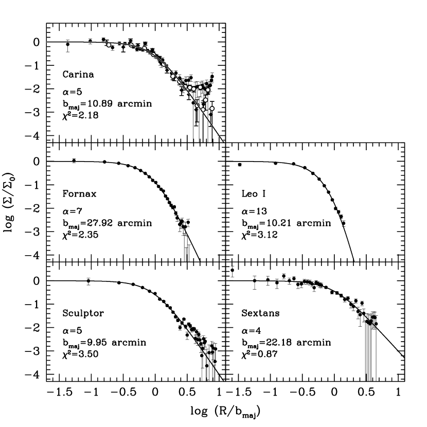
Figure 1.— Normalized radial surface brightness profiles. Points with error bars show the observed star counts; the lines show the best fitting generalized Plummer models. For Carina, the data from Irwin & Hatzidimitriou (1995), Majewski et al. (2000), and Muñoz et al. (2006) are shown as filled circles, empty circles, and diamonds, respectively.

For the five dSphs analyzed in this paper, I obtained the generalized Plummer profile parameters, $b$ and $\alpha$, by $\chi^{2}$ fitting of eq. (5) to the best available star count data: Coleman et al. (2005b, their Figure 15) for Fornax, Smolčić et al. (2007, their Figure 9) for Leo I, Coleman et al. (2005a, their Figure 6) for Sculptor, and Irwin & Hatzidimitriou (1995) for Sextans. For Carina, there were significant discrepancies between the published star count profiles, so I carried out a joint $\chi^{2}$ fitting for three different datasets: Irwin & Hatzidimitriou (1995), Majewski et al. (2000, their Table 3), and Muñoz et al. (2006, their Figure 4b). As the fitting was done in the linear space, all star count data points (even those which became formally negative after subtracting the assumed contribution from the background sources) were used. Figure 1 shows the star count data and the best fitting generalized Plummer models for the five dSphs.

Table 1$\chi^{2}$ for different surface brightness models

Galaxy	$\chi^{2}_{\rm GP}$	$\chi^{2}_{\rm P}$	$\chi^{2}_{\rm EK}$	$\chi^{2}_{\rm S}$
Carina	2.18	2.18	2.83	2.92
Fornax	2.35	9.81	2.86	2.55
Leo I	3.12	47.8	11.5	6.66
Sculptor	3.50	3.50	4.86	4.98
Sextans	0.87	1.03	0.84	0.89
Draco	0.65	1.69	1.25	1.10
Average	2.11	11.0	4.02	3.18

Table 1 presents the best $\chi^{2}$ values (normalized by the number of degrees of freedom) for the five dSphs for four different profiles (generalized Plummer, classical Plummer, empirical King, and Sérsic); I also included the fitting results for the Draco data from Odenkirchen et al. (2001, their sample S2) – the same data we used in Mashchenko et al. (2006a) for mass modeling of this galaxy. As you can see in Table 1, the generalized Plummer profile is the best one overall: for each galaxy, it produces the same or better fit than the other profiles, and is significantly better in terms of the average $\chi^{2}$ for all the six dwarfs. I warmly recommend this profile for all future dSph mass modeling work, as it is simple (surface and volume densities and gravitational potential are simple analytical expressions – as long as $\alpha$ is an integer) and appears to be the best fitting profile among 2–3 parameter models.

One complication is that all the published star count profiles were computed inside elliptical annuli (usually with the fixed ellipticity $e$ and position angle), with the quoted radius measured along the major axis of the galaxy. For the purposes of this study, spherically averaged (in the plane of the sky) surface brightness profiles are required. For each galaxy, I computed the spherically averaged profile by solving numerically the following integral for 100 values of the projected radius $R=0.001\dots 30$:

$$\Sigma_{\rm avr}(R)=\frac{2}{\pi}\int\limits_{0}^{\pi/2}\left(1+\frac{R^{2}}{\cos^{2}\varphi+(1-e)^{2}\sin^{2}\varphi}\right)^{-\frac{\alpha-1}{2}}{\rm d}\varphi.$$ (7)

Here $e$ is the ellipticity of the galaxy. The resultant, averaged profile is very close (but not identical) to the generalized Plummer profile with the same exponent $\alpha$ and a smaller core radius $b$. I derived this spherically averaged value of $b$ by $\chi^{2}$ fitting the above profile with the generalized Plummer profile. The correction factor $b/b_{\rm maj}$ is a function of both $e$ and $\alpha$, and ranges from 0.816 (Sextans) to 0.895 (Leo I). (Here $b_{\rm maj}$ is the core radius obtained from fitting the generalized Plummer model to the original data, before averaging.)

Table 2Input galactic parameters

Galaxy	$D$	$\Sigma_{0}$	$e$	(M/L)∗	$V_{\rm sys}$	$\alpha$	$b_{\rm maj}$	$b$	$\rho_{*,0}$	$R_{\rm hl}$
	kpc	mag arcsec-2		M⊙/L⊙	km s-1		arcmin	arcmin	M⊙ pc-3	arcmin
Carina	101	25.5	0.33	0.845	222.9	5	10.89	9.00	0.0055	3.97
Fornax	138	23.4	0.31	0.935	55.2	7	27.92	23.61	0.0147	7.67
Leo I	255	22.6	0.21	0.74	282.9	13	10.21	9.14	0.0490	1.92
Sculptor	79	23.7	0.32	1.23	111.4	5	9.95	8.28	0.0584	3.66
Sextans	86	26.2	0.35	1.15	224.3	4	22.18	18.09	0.00195	10.45

The results of the generalized Plummer profile fitting and other input galactic parameters for the five dSphs are presented in Table 2. As this study properly takes into account the self-gravity of stars, I had to assume certain values for the stellar mass-to-light ratios in $V$-band, (M/L)_∗. For each galaxy, I used the average of the Salpeter and composite (M/L)_∗ estimates of Mateo et al. (1998, their Table 6). Knowing the distance to the galaxy, $D$, the $V$-band central surface brightness, $\Sigma_{0}$, the generalized Plummer model parameters $\alpha$ and $b$, and (M/L)_∗ allowed me to compute the central stellar density, $\rho_{*,0}$ (see Table 2). The table also lists the estimated half-light radii (in arc minutes), $R_{\rm hl}$, for spherically averaged models.

3.2. Line-of-sight star velocities

I used the stellar line-of-sight velocities catalogs of Walker et al. (2009a) for Carina, Fornax, Sculptor, and Sextans, and the catalog of Mateo et al. (2008) for Leo I. These are the largest homogeneous catalogs available for dwarf spheroidals, with the number of stars per galaxy ranging from $\sim 300$ (Leo I) to $\sim 2500$ (Fornax). I used the merged version of the data. The median error of the velocity measurements is $\pm 2.1$ km s^-1. In all the dwarfs (except for Leo I) some contamination from foreground Galactic stars is expected to be present in the data. Walker et al. (2009b) quantified this contamination by computing individual “membership probabilities” $P$ for each star. For this study, I only used stars with $P>0.95$ for Carina, Sculptor, and Sextans, and stars with $P>0.75$ for Fornax. (Despite the less conservative selection criterion for Fornax, the resultant line-of-sight dispersion profile looks very smooth and un-contaminated, and the normalized $\chi^{2}$ for the best fitting model is $\sim 1$ – see Figure 2.) Due to the Leo I’s large heliocentric velocity and distance from the Sun, the data for this dwarf should have essentially zero contamination in the range of heliocentric velocities from 260 to 315 km s^-1 (Walker et al., 2007, their Fig. 1). Accordingly, I used these simple velocity cuts to select the Leo I star candidates.

Carina was the only galaxy in our sample for which the best fitting model deviated more than two sigmas from the data. This could be due to unaccounted foreground contamination (which would not be surprising, given that it is the closest to the Galactic plane dSph and has a very low surface brightness). For this galaxy only, I removed the six stars (after removing the stars with $P<0.95$), for which the deviation from the best fitting model was more than three sigmas, and then repeated the full mass modeling for the reduced star list. (Here one sigma corresponds to the total, model $+$ observational uncertainty, velocity dispersion.) The removed stars have the following designations in the Walker et al. (2009a) catalog: Car-0056, 0200, 0465, 0547, 0680, 1892. This operation boosted the absolute probability of the best fitting model for Carina from 0.04 to 0.26 (when $N_{\rm bin}=7$; see § 4.3). It is important to note that all the six stars are located in the outer half of the radial bins, so this operation should have had very little impact on the analysis of the central parts of the galaxy – which is the main focus of the current study.

4. CHOOSING GOOD MODELS

4.1. $\chi^{2}$ fitting

Two popular statistical methods used in mass modeling of dSphs are $\chi^{2}$ fitting and maximum likelihood analysis. Both methods have advantages and disadvantages. The $\chi^{2}$ method complements naturally the Jeans analysis, as both operate only with the second moment (dispersion) of the stellar velocity distribution, whereas for the maximum likelihood approach one has to assume a certain (usually Gaussian) form for the line-of-sight velocity probability distribution function. This factor makes the $\chi^{2}$ fitting less sensitive to outliers, and hence a much better approach when one is interested in absolute probabilities of different models. The maximum likelihood method, on the other hand, is more appropriate for post-Jeans mass modeling, where the full model line-of-sight velocity PDF is computed and compared to the data.

The main disadvantages of the $\chi^{2}$ technique are that 1) one has to try a few different values for the number of the radial bins, $N_{\rm bin}$ – but that only means longer computing time, and 2) in its simplest implementation, the random locations of individual stars within each radial bin is an additional source of variance in the analysis. To address the latter issue, for both the observational data and model I estimate the following quantity (for each radial bin):

$$S=\frac{1}{n}\sum_{i=1}^{n}\sigma_{i}^{2}.$$ (8)

Here $\sigma_{i}$ is the line-of-sight velocity dispersion at the specific location (projected distance from the dwarf’s center) of the $i$-th star, and $n$ is the number of stars in the current radial bin. The quantity $S$ will converge to the square of the local line-of-sight velocity dispersion when the radial extent of the bin shrinks to zero and the number of stars ($n$) grows to infinity. The important point is that such a convergence is not required when all one wants to do is to measure the statistical deviation of the model from the data. All is needed is to estimate the mean (for the data and the model) and standard deviation (only for the data) of the quantity $S$ for each radial bin, and then compute the $\chi^{2}$ deviation for $S$ from all the radial bins. As the $S$ measurements for both observational data and model are carried out for the same projected distances from the center of the dwarf (corresponding to the distances of actual stars), the variance due to random locations of stars within radial bins is completely removed.

Of course, we do not know from the observations the values of $\sigma_{i}$ at the position of each star. Instead, we know the individual line-of-sight velocities (corrected for the systemic velocity of the galaxy), $V_{i}$, and the associated measurement uncertainties, $\sigma_{{\rm mes},i}$. One can use these known quantities to write down the following unbiased estimator of $S$ (without any assumptions on the shape of the velocity PDF):

$$\hat{S}=\frac{1}{n}\sum_{i=1}^{n}\left(V_{i}^{2}-\sigma_{{\rm mes},i}^{2}\right).$$ (9)

This expression is valid even for the cases when the line-of-sight velocity dispersion changes dramatically within a single radial bin. The standard deviation of $\hat{S}$ can be estimated from the following expression,

$$\sigma_{S}\simeq\frac{1}{n}\left[2\sum_{i=1}^{n}\left(\hat{S}+\sigma_{{\rm mes},i}^{2}\right)^{2}\right]^{1/2},$$ (10)

which does require the velocity dispersion to be approximately constant within a single bin. Numerical experiments showed that eq. (10) noticeably deviates from the true answer only when the velocity dispersion changes significantly (by a factor of two or more) within a single radial bin, which is never the case in my best fitting models.

Eqs. (8–10) are written for a single radial bin. It is now straightforward to write down the expression for the $\chi^{2}$ deviation of the model from the data for all the $N_{\rm bin}$ radial bins:

$$\chi^{2}_{k}=\sum_{j=1}^{N_{\rm bin}}\left(\frac{\hat{S}_{j}-S_{j}}{\sigma_{S,j}}\right)^{2}.$$ (11)

Here $S_{j}$, $\hat{S}_{j}$, and $\sigma_{S,j}$ are computed for the $j$-th radial bin using eqs. (8), (9), and (10), respectively, and $k=N_{\rm bin}-\lambda$ is the number of the statistical degrees of freedom, where $\lambda$ the effective dimensionality of the free parameter space (see § 4.2).

The only drawback of the above procedure is that it can be substantially more computationally expensive than the standard $\chi^{2}$ analysis, as one has to compute the model line-of-sight velocity dispersion (numerical integration using eq. (4)) for each model, each star, and each value of $N_{\rm bin}$.

4.2. Artificial data tests

One can already use eq. (11) from the previous section to compute the relative goodness of fit for different models. To go one step further and convert the $\chi^{2}$ values to the absolute probabilities of the models,

$$\Pi=P\left(\frac{k}{2},\frac{\chi^{2}_{k}}{2}\right),$$ (12)

one has to estimate the effective number of dimensions of the free parameter space, $\lambda$. (Here $P(x,y)$ is the regularized Gamma function.)

To estimate $\lambda$ for my six-parameter model described in § 2, I generated a dataset of 2499 fake stars located at the same projected distances from the dwarf’s center as the real 2499 stars in Fornax with known line-of-sight velocities (see § 3.2). I used my best fitting Fornax model (for the $N_{\rm bin}=7$ case) and actual individual star velocity observational uncertainties, $\sigma_{\rm mes}$, to generate random values of the “observed” line-of-sight velocities for the artificial stars. (I assumed that both the model line-of-sight velocities and the observational velocity uncertainties have Gaussian distributions.)

Next, I split my artificial dataset into 21 equal size sub-sets (each one consisting of 119 randomly selected fake stars). In a sense, I generated 21 random realizations of the Fornax galaxy. Then I carried out full mass modeling (as described in § 4.3, with $N_{\rm bin}=7$) and derived the $\chi^{2}_{k}$ value (eq. (11)) for the best fitting model, separately for each sub-set. Assuming that the resultant 21 random numbers are drawn from the same $\chi^{2}_{k}$ distribution, their mean should be an unbiased estimator for $k$. In this numerical experiment, I derived $k\simeq 3.73$, corresponding to the effective number of dimensions in my free parameter space $\lambda=N_{\rm bin}-k\simeq 3.27$. I used this number in the rest of the paper. This number is significantly (almost by a factor of two) lower than the formal number of the model free parameters (six) reflecting significant degeneracies (from the Jeans analysis point of view) present in the model. As one will see in § 5, the most degenerate is the parameter $\gamma$ (the logarithmic slope of the DM density). Post-Jeans mass modeling (dealing with the full line-of-sight velocity PDF, and not just with the dispersion) is expected to be less degenerate.

It is clear that $\lambda$ will not be exactly the same for different data and for different number of radial bins (because the radial extent of the binned data depends on $N_{\rm bin}$), but as long as the number of bins is relatively large (so that $k=N_{\rm bin}-\lambda\gg 1$), the computed absolute probabilities should not be very sensitive to the errors in $\lambda$. To be more quantitative, I computed numerically the relative error for the absolute probabilities $\Pi$ resulting from the $\lambda$ uncertainty, $(\Delta\lambda/\Pi)\>{\rm d}\Pi/{\rm d}k$, for $k=3.73$ and two different cases: $\chi^{2}_{k}=k$ (corresponding to $\Pi\simeq 0.4$, as in my best fitting models), and $\chi^{2}_{k}=2.5k$ (corresponding to $\Pi\simeq 0.04$, my lower cutoff for “good models”). Purely statistical (Poissonian) errors in estimating $k$ (and hence $\lambda$) from the limited sample of the size $N_{S}=21$ is of the order of $(2k/N_{S})^{1/2}\simeq 0.6$. Assuming a larger uncertainty (to account for a variance in data) $\Delta\lambda=1$, the resulting relative errors in $\Pi$ are only $0.05$ and $0.35$, respectively, which I consider to be acceptable. If $N_{\rm bin}>7$, as is the case with most of my galaxies, the relative errors in $\Pi$ should be significantly smaller.

Figure 2.— Radial line-of-sight stellar velocity dispersion profiles. Solid circles with error bars show the binned observational data. The solid and dotted lines show the best models with $\gamma=0$ and 1, respectively.

4.3. Numerical algorithm

In this section I outline my overall mass modeling procedure.

I thoroughly explored (“brute force optimization”) the four out of the six free model parameters: the central logarithmic DM density slope $\gamma$, and the three stellar anisotropy parameters, $\eta_{0}$, $\eta_{1}$, and $r_{a}$ (see § 2). For $\gamma$, I used the discrete values (0, $0.1$, $0.2$, …, $1$), which covered the whole plausible range – from the observations-suggested flat core ($\gamma=0$) to the CDM prediction, $\gamma\sim 1$. In these low stellar density objects the presence of baryons is not expected to make the DM distribution “cuspier” via the adiabatic contraction of DM. A presence of a sufficiently massive central black hole could have steepened the DM cusp, but there is no evidence for super-stellar mass black holes in dSphs (Lora et al., 2009).

Both $\eta_{0}$ and $\eta_{1}$ had the following discrete values: ($-1$, $-0.9$, $-0.8$, …, 1), which covered the full range of anisotropies – from purely tangential ($\eta=-1$) to purely radial ($\eta=1$). In addition, for the central anisotropy $\eta_{0}$ I only explored the range allowed by the central anisotropy theorem of An & Evans (2006), $\eta_{0}\leqslant(4/\gamma-1)^{-1}$. The anisotropy radius $r_{a}$ had the following values (in the units of the stellar core radius $b$): (0.1, 0.147, 0.215, 0.316, 0.464, 0.681, 1.47). They are equidistant in the logarithmic space, and span the full range of radial distances resolved by the data. Overall, I explicitly tested 22,344 different models with the above discrete values of the four model parameters.

The remaining two model parameters, DM halo scaling radius $r_{s}$ and density $\rho_{s}$, are very well constrained by the data when the rest of the parameters are fixed, which allowed me to use implicit optimization technique for these two parameters. This dramatically reduced the number of models to be tested and hence the total computational time, as $r_{s}$ and especially $\rho_{s}$ span a very large range of values (four orders of magnitude for $\rho_{s}$, see Table 3). The only prior was for $r_{s}$ to stay within the interval 0.05 …5 (in $b$ units; for Sculptor, I used a different range 0.1 …15, as this galaxy has a very compact core). There was no prior for $\rho_{s}$.

I used the one-dimensional Brent’s method (Press et al., 1992) separately for $r_{s}$ and $\rho_{s}$ optimization (finding global minimum in $\chi^{2}_{k}$; $\rho_{s}$ optimization is the inner loop, and $r_{s}$ optimization is the outer loop). The method showed a good numerical convergence, requiring only of order of a hundred models with different combinations of ($r_{s}$, $\rho_{s}$) to be tested (when the other four explicit parameters were fixed). Including both explicitly and implicitly explored parameters, I had to compute the $\chi^{2}_{k}$ deviation from the data for $\sim 2\times 10^{6}$ different models – per galaxy and per $N_{\rm bin}$ value.

For a given galaxy and a chosen combination of the six model parameters and the value of $N_{\rm bin}$, I solved the Jeans eq. (1) numerically, and then solved numerically the integral in eq. (4) to derive $\sigma_{\rm los}$ at all the projected radii $R$ corresponding to the locations of the dwarf’s stars with known line-of-sight velocity. Then I used eqs. (8–11) to compute the $\chi^{2}$ deviation of the model from the data, and eq. (12) to assign absolute probabilities to the models.

Absolute probabilities of the best fitting models, $\Pi_{\rm max}$, range from 0.23 for Sculptor to 0.60 for Sextans (Table 3), corresponding to $\sim 0.5-1.2$ sigma deviations. I used one global lower cut-off value of $\Pi_{\rm low}=0.0455$ (a two sigma deviation) to select good models for all the galaxies.

I used the following approach to determine the optimal value of the number of radial bins, $N_{\rm bin}$, for each galaxy. In the limit of large $N_{\rm bin}$ (small number of stars in one bin, $n$), $\sigma_{S}\propto N_{\rm bin}^{1/2}$ (see eq.(10)) and the $\chi^{2}$ analysis becomes dominated by the Poissonian noise and hence “fuzzier” (less discriminatory). In the opposite limit, $N_{\rm bin}\rightarrow 0$, the signal to noise ratio improves, but the $\chi^{2}$ analysis becomes again less accurate because with fewer radial bins we start loosing radial resolution and may overlook some sharp $\sigma_{\rm los}$ features near the dwarf’s center or in the galactic outskirts. In addition, when $N_{\rm bin}$ approaches $\lambda$ (the effective dimensionality of the free parameter space), the errors in measuring $\lambda$ become more important, which makes the absolute model probabilities less reliable (see § 4.2). Hence it appears there should be a certain value of $N_{\rm bin}$ when the $\chi^{2}$ analysis is the most accurate (or discriminatory). I found this optimal value separately for each galaxy by running the full set of models for $N_{\rm bin}=7$ (minimum acceptable number of bins for this model, see § 4.2), 15, and 30, and then choosing the value which produced the smallest fraction of good models ($f_{2\sigma}$ in Table 3). For Fornax, Sculptor, and Sextans the optimal value of $N_{\rm bin}$ was found to be 15; for Carina and Leo I it is equal to 7 (Table 3).

5. RESULTS

I applied the mass modeling procedure described in the previous sections to all the five dwarfs. The full results are available online. As good models found in the current analysis occupy only a small fraction of the total six-dimensional free parameter space, the data presented here can be used for post-Jeans mass modeling projects (utilizing the full PDF of the observed stellar line-of-sight velocities; the subject of Paper II) to dramatically reduce the required computational time.

Figure 2 shows the radial $\sigma_{\rm los}$ profiles for the two best-fitting models (with $\gamma=0$, solid lines, and $\gamma=1$, dotted lines) for each galaxy. As one can see, the overall quality of the model fits is excellent, with the $\chi^{2}$ values (normalized by the number of degrees of freedom $k=N_{\rm bin}-\lambda$) being close to a unity. It is remarkable that these two dramatically different values of $\gamma$ (0 and $1$) make very little difference in the quality of the model fit. This is most obvious for the galaxy with the highest quality data – Fornax – where the two $\sigma_{\rm los}$ profiles are essentially identical way beyond the radial range covered by the data. For the galaxies with the best $\gamma=0$ and $\gamma=1$ profiles apparently diverging near the center (Sculptor and Sextans), one could naïvely think that with a larger $N_{\rm bin}$ (and hence with the binned data covering a wider range of radial distances) the two models would become more statistically distinct. But this is not the case: for all the values of $N_{\rm bin}$ I tried (7, 15, and 30), and for all the five galaxies, the difference between the best fitting models with different values of $\gamma$ is statistically insignificant, to a similar degree.

Table 3Global constraints

Name	$N_{*}$	$N_{\rm bin}$	$f_{2\sigma}$	$\Pi_{\max}$	$\eta_{0}$	$r_{s}$	$\rho_{s}$	$\rho_{0,{\rm min}}$	$(M/L)_{0,{\rm min}}$
								$M_{\odot}$ pc-3	$M_{\odot}/L_{\odot}$
Carina	740	7	0.680	0.262	$-1\dots 0.3$	$0.05\dots 5$	$1.7\dots 2.5\times 10^{4}$	0.048	8.2
Fornax	2499	15	0.253	0.468	$-0.8\dots 0.3$	$0.05\dots 5$	$0.25\dots 2.1\times 10^{3}$	0.028	2.7
Leo I	328	7	0.210	0.302	$-0.8\dots 0.3$	$0.05\dots 5$	$0.13\dots 600$	0.080	1.95
Sculptor	1349	15	0.230	0.228	$-0.9\dots 0.3$	$0.5\dots 15$	$0.16\dots 63$	0.087	3.1
Sextans	397	15	0.906	0.598	$-1\dots 0.3$	$0.05\dots 5$	$0.90\dots 2.9\times 10^{4}$	0.007	5.3

Table 4Radius-dependent constraints

Name	$r_{1}$	$M_{1}$	$(M/L)_{1}$	$r_{2}$	$\rho_{\rm DM}$	$(M/L)_{2}$	$r_{3}$	$\eta$	$M_{300}$	$M_{600}$
	pc	$10^{7}M_{\odot}$	$M_{\odot}/L_{\odot}$	pc	$M_{\odot}$ pc-3	$M_{\odot}/L_{\odot}$	pc		$10^{7}M_{\odot}$	$10^{7}M_{\odot}$
Carina	409	0.74…1.14	26…39	187	0.032…0.074	14…32	…	$-1$…0.3	0.35…0.78	0.85…2.3
Fornax	924	6.1…8.0	5.5…6.9	453	0.021…0.040	3.7…6.2	232	$-0.88$…0.05	0.27…3.4	1.90…5.1
Leo I	389	1.55…1.94	3.4…4.1	204	0.067…0.115	2.5…3.8	72	$-0.67$…0.26	0.76…1.43	1.94…5.7
Sculptor	435	2.17…3.01	22…30	256	0.067…0.107	20…31	83	$-0.46$…0.19	0.79…1.63	2.9…5.8
Sextans	1034	1.4…3.2	19…42	451	0.004…0.013	11…32	…	$-1$…0.3	0.06…1.1	0.37…1.7

Tables 3 and 4 summarize the main results of this study. In particular, I list there the ranges spanned by good ($<2\sigma$) models separately for the free model parameters $\eta_{0}$, $r_{s}$, and $\rho_{s}$. As one can see, these parameters are very poorly constrained by the Jeans analysis. The full allowed range for $\eta_{0}$ is $-1\dots 0.3$ (due to the An & Evans 2006 central anisotropy theorem), and only three galaxies (Fornax, Leo I, and Sculptor) have a (very weak) constraint on this parameter, in the sense that the pure central tangential anisotropy is excluded. Similarly, only one galaxy (Sculptor) has any constraints on the DM halo scaling radius: $r_{s}\gtrsim 0.5$ (in $b$ units). For the rest of the dwarfs, good models span the full explored range of $r_{s}$, from 0.05 to 5. Parameter $\rho_{s}$ is the only one in the current analysis which is allowed to take any values (no priors), so it does appear to be constrained in a meaningful way. One has to remember though that there is a strong degeneracy between $\rho_{s}$ and $r_{s}$. E.g., if $r_{s}$ were allowed to go to even smaller values ($<0.05$), the range for $\rho_{s}$ would expand to even larger values. I do not list global constraints for the three remaining model parameters, $\gamma$, $\eta_{1}$, and $r_{a}$, as good models span the full ranges for these parameters: $0\dots 1$, $-1\dots 1$, and $0.1\dots 1.47$, respectively. The conclusion here is that in mass modeling of dwarf spheroidal galaxies the Jeans analysis is not capable of placing meaningful constraints on global model parameters (for models which are flexible enough, as in the current study).

The analysis does constrain the minimum central DM density, $\rho_{\rm 0,\rm min}$, and the corresponding mass to light ratio, $(M/L)_{0,\rm min}$ (see Table 3). Sculptor and Leo I have the strongest constraints on $\rho_{\rm 0,\rm min}$ ($\gtrsim 0.09$ M_⊙ pc^-3 and $\gtrsim 0.08$ M_⊙ pc^-3, respectively, at the two-sigma level). Carina, on the other hand, has the strongest $(M/L)_{0,\rm min}$ constraint: $\gtrsim 8$ M${}_{\odot}/$L_⊙.

Figure 3.— Averaged DM density, $\rho_{\rm avr}$, as a function of radius, $r$, in stellar units ($\rho_{*,0}$ and $b$, respectively). Two solid lines outline the range of the models consistent with the observational data at better than $2\sigma$ level. Dashed lines correspond to formally best models. Vertical dotted lines mark the radius ($r_{1}$ in Table 3) where the $\rho_{\rm avr}$ uncertainty is the smallest. Dash-dotted lines show the averaged density profiles for stars.

More useful constraints can be derived for radius-dependent (computed at different distances from the dwarf’s center) quantities. Figure 3 plots the range of the averaged DM density $\rho_{\rm avr}$ spanned by good models as a function of the enclosed radius $r$, separately for each galaxy. The averaged stellar density profiles (dash-dotted lines) are shown for comparison. There has been a debate in the literature (Mateo et al., 1993; Strigari et al., 2007, 2008; Walker et al., 2009c; Wolf et al., 2009) regarding the value of the radius at which the Jeans analysis provides the tightest constraints on the enclosed mass (or equivalently the averaged density). As one can see in Figure 3, such radius indeed exists (vertical dotted lines) and is very well defined. In Table 4 I list these radii ($r_{1}$), the range of the enclosed mass spanned by good models at those radii ($M_{1}$), and also the corresponding range of the mass-to-light ratio ($(M/L)_{1}$), for all the dwarfs. For comparison, in Table 4 I also list the good model ranges of the enclosed mass at 300 and 600 pc – $M_{300}$ and $M_{600}$, respectively. As one can see, $r_{1}$ ranges widely, from 390 pc for Leo I to more than 1000 pc for Sextans, and at neither of the previously suggested radii (300 and 600 pc) the enclosed mass is well constrained by the Jeans analysis for all the dwarfs. To be more quantitative, the mean-squared two-sigma error for all the five dwarfs is $\pm 0.40$ dex, $\pm 0.24$ dex, and $\pm 0.10$ dex ($\pm 25\%$) for the enclosed mass measured within 300 pc, 600 pc, and $r_{1}$ (unique for each galaxy), respectively. The accurately determined values of the enclosed mass presented here can be very useful for identifying the dSph counterparts in cosmological simulations, and is probably the most important result of the current study.

The conjecture of Walker et al. (2009c) that the enclosed mass is well constrained at the half-light radius, $R_{\rm hl}$, is not corroborated by the current study. In fact, enclosed masses measured at this radius result in the worst mean-squared two-sigma error, $\pm 0.58$ dex.

The conclusion of Wolf et al. (2009) (whose analysis is hard to interpret, as DM and stars are coupled in their model) that the enclosed mass has the best constraint at the radius where $\gamma_{*}\equiv-{\rm d}\log\rho_{*}/{\rm d}\log r=3$ is also not borne out in the current study: for the five dwarfs I obtained $\gamma_{*}=3.54\pm 0.38$ at my best radii ($r_{1}$), with the full range from 3.22 to 4.20. My sample of galaxies is too small to try to find a good estimator for $r_{1}$, but I believe it should be a function of both the stellar density profile ($\gamma_{*}(r)$) and the quality and quantity of the stellar line-of-sight velocity measurements. This issue needs to be explored further once a larger sample of dwarfs is subjected to a similar analysis.

To estimate how sensitive the above analysis is to particular values of $N_{\rm bin}$, I repeated it for all the three values of $N_{\rm bin}$: 7, 15, and 30. For the less optimal values of $N_{\rm bin}$, the radii where the enclosed mass is measured to the highest possible accuracy ($r_{1}$) does not deviate from the value obtained with the optimal $N_{\rm bin}$ by more than 7% (for Sextans; for Fornax it is essentially zero). The averaged DM density measured at $r_{1}$ is also very close for all the values of $N_{\rm bin}$ (less than one sigma deviation), with one notable exception: for Leo I, moving from $N_{\rm bin}=7$ (the optimal value) to $N_{\rm bin}=30$ results in $\rho_{\rm avr}(r_{1})$ becoming smaller by 0.18 dex, or $3.8\sigma$. (This may be related to the fact that Leo I has the smallest number of stars with a known line-of-sight velocity: $N_{*}=328$.) Overall, this analysis seems to be largely insensitive to how well the optimal value of $N_{\rm bin}$ is chosen.

Another proposition discussed in the literature is that there is a radius (300 pc) at which the enclosed mass is the same for all dwarf spheroidals – around $10^{7}$ M_⊙ (Mateo et al., 1993; Strigari et al., 2008). This is barely (at $2\sigma$ level) consistent with the data in the current analysis, as there is a tension between Carina on one side, and Leo I and Sculptor – on the other side (see Table 4). The galaxies may have a similar mass at this radius, but it is unlikely to be identical. If one considers even smaller radii (say, 200 pc), then formally there will be a common enclosed mass for all the five dwarfs consistent with the data at better than two sigma level, but only because the uncertainties in measuring the enclosed mass increase dramatically at smaller radii (see Figure 3).

Figure 4.— Local DM density, $\rho$, as a function of radius, $r$, in stellar units ($\rho_{*,0}$ and $b$, respectively). Two solid lines outline the range of the models consistent with the observational data at better than $2\sigma$ level. Dashed lines correspond to formally best models. Vertical dotted lines mark the radius ($r_{2}$ in Table 3) where the $\rho$ uncertainty is the smallest. Dash-dotted lines show the density profiles for stars.

Another interesting radius-dependent quantity, local DM density, is more model dependent, and is not as well constrained by the Jeans analysis as the enclosed mass. Figure 4 shows the ranges for $\rho_{\rm DM}(r)$ spanned by good models. I also plot there the stellar density profiles, $\rho_{*}(r)$, as dash-dotted lines. As with the averaged density case, each galaxy has a well defined radius, $r_{2}$, (vertical dotted lines) where the local DM density is best constrained by the data. Table 4 lists the values of $r_{2}$ and the corresponding ranges of $\rho_{\rm DM}(r_{2})$ and the local mass-to-light ratio $(M/L)_{2}$ for each galaxy. $r_{2}$ tends to be a factor of two smaller than $r_{1}$. The uncertainty in $\rho_{\rm DM}(r_{2})$ ranges from 0.20 dex for Sculptor to 0.5 dex for Sextans, which is substantially worse than the constraints on the enclosed mass. Still, knowing the local DM density at a certain radius (which happens to be quite small) to a reasonably good accuracy can be very useful – for example, for studies aimed at direct search of DM in dwarf spheroidals via its annihilation signal. Both Figures 3 and 4 clearly demonstrate that these dSphs are DM dominated at all radii.

Figure 5.— Stellar anisotropy, $\eta$, as a function of radius, $r$ (in units of $b$). Two solid lines outline the range of the models consistent with the observational data at better than $2\sigma$ level. Two dotted lines show the total allowed range of models. Dashed lines correspond to formally best models. Vertical dotted lines mark the radius ($r_{3}$ in Table 3) where the $\eta$ uncertainty is the smallest.

The last radius-dependent quantity which has useful (albeit very weak) constraints is the local stellar velocity anisotropy, $\eta(r)$. Figure 5 demonstrates that better than two sigma models span a wide range of $\eta$ at each radius $r$, which is only slightly narrower than the full allowed range (the space between the two dotted lines). The best radius, $r_{3}$, is not as well defined as with $\rho_{\rm avr}(r)$ and $\rho_{\rm DM}(r)$. I list the values of $r_{3}$ and the corresponding good model ranges for $\eta(r_{3})$ in Table 4. Sculptor has the tightest constraints on $\eta(r_{3})$; Carina and Sextans are essentially unconstrained.

Given how poor the constraints on $\eta(r)$ are, very little can be learned from the analysis of Figure 5. One interesting conclusion is that at any given radius the data are consistent with stellar velocities being isotropic ($\eta(r)=0$). One cannot conclude from this radius-dependent analysis that the global stellar isotropy is also consistent with the data. To address the latter issue, one has to analyze the full results of the current study (available online). Specifically, one has to test if all the globally isotropic models (with $\eta_{0}=\eta_{1}=0$) are good ones (deviate less than $2\sigma$ from the data). I carried out such an analysis, with the conclusion being that indeed the data is consistent (at better than $2\sigma$ level) with the global stellar velocity isotropy hypothesis for all the dwarfs.

It has already been demonstrated (Strigari et al., 2008; Walker et al., 2009c) that in dSphs the central logarithmic DM density slope, $\gamma$, is not constrained by the Jeans analysis (when no stellar proper motion data are available). My analysis generalizes this result for all radii $r$: the local logarithmic DM density slope, $\gamma(r)=-{\rm d}\log\rho_{\rm DM}/{\rm d}\log r$, is found to be unconstrained by the Jeans analysis.

6. CONCLUSIONS

I carried out the classical Jeans mass modeling of the five dwarf spheroidal galaxies with the highest quality observational data – Carina, Fornax, Leo I, Sculptor, and Sextans. My primary goal was to push the analysis to its limits, by developing a flexible enough galactic model (with variable stellar velocity anisotropy), refining the traditional $\chi^{2}$ fitting algorithm, and investing a significant amount ($3\times 10^{5}$ cpu hours) of supercomputing time to carry out an exhaustive model parameter optimization. The main results of this study are as follows.

• My galactic model with the six free parameters ($r_{s}$, $\rho_{s}$, $\gamma$, $\eta_{0}$, $\eta_{1}$, and $r_{a}$) gives a good description of the observational data: the normalized $\chi^{2}$ for the differences between the model and observed velocity dispersion profiles are close to a unity, which is consistent with the deviations being purely due to the observational errors.

• I show that the Jeans mass modeling approach (even with high quality data and modeling) cannot place meaningful constraints on most galactic parameters, including the central DM density logarithmic slope ($\gamma$), DM halo scaling radius ($r_{s}$) and density ($\rho_{s}$), and central stellar velocity anisotropy ($\eta_{0}$). Moreover, I show that the local DM density logarithmic slope, $\gamma(r)=-{\rm d}\log\rho_{\rm DM}/{\rm d}\log r$, is unconstrained at all the radii probed by the data. As a consequence, one must resort to much more computationally expensive post-Jeans mass modeling techniques (which deal with the full probability distribution function for stellar line-of-sight velocities, and not just the dispersion) to be able to solve the “cusp – core” issue for dSphs, or to identify theoretical mechanisms responsible for flattening DM cusps in dwarf galaxies (by constraining the stellar velocity anisotropy profiles).

• My most important finding is that there is a certain radius ($r_{1}$; different for each galaxy) where Jeans mass modeling provides the tightest constraints on the enclosed mass in dSphs. For Carina, Fornax, Leo I, Sculptor, and Sextans my two-sigma constraints for the enclosed DM mass are $0.74\dots 1.14\times 10^{7}$ M_⊙ (at 409 pc), $6.1\dots 8.0\times 10^{7}$ M_⊙ (at 924 pc), $1.55\dots 1.94\times 10^{7}$ M_⊙ (at 389 pc), $2.17\dots 3.01\times 10^{7}$ M_⊙ (at 435 pc), and $1.4\dots 3.2\times 10^{7}$ M_⊙ (at 1034 pc), respectively. These constraints are much tighter than the constraints at the previously suggested “good” radii – 300 pc, 600 pc, and the half-light radius. The tight constraints can be very valuable for placing the dSphs in the proper cosmological context.

• I also derive useful constraints on the local DM density. Similarly to the enclosed mass, each galaxy has a certain radius ($r_{2}$) where my Jeans analysis places the tightest constraints on this quantity. For example, I show that in Sculptor $\rho_{\rm DM}=0.067\dots 0.107$ $M_{\odot}$ pc^-3 (two-sigma interval) at 256 pc from its center. Also, the analysis produced useful minimum central DM density ($\rho_{0,{\rm min}}$) constraints (the largest one is for Sculptor: $\rho_{0}\gtrsim 0.09$ $M_{\odot}$ pc^-3). These constraints can be used in projects aimed at detecting DM in dSphs via its annihilation signal.

• I show that stellar anisotropy profiles are very poorly constrained in Jeans mass modeling. The only useful results here are that the pure central tangential anisotropy is excluded at better than two-sigma level for three out of the five dSphs, and that the data are consistent with the global stellar velocity isotropy for all the five dwarfs.

• A significant advantage of the exhaustive search through the multi-dimensional model parameter space employed in this study, with all the intermediate results stored and available online, is that the results can be used for many other projects. Most importantly, this analysis can be used as the first preliminary step (which eliminates a vast majority of models which are incompatible with the data) in post-Jeans mass modeling projects (which model the full PDF for the stellar line-of-sight velocities) – the subject of my Paper II in this series. The latter approach should be able to overcome most of the degeneracies present in Jeans mass modeling (as exposed in the current work), hopefully settling once and for all whether dSphs have flat DM cores.

References

- Aaronson (1983) Aaronson, M. 1983, ApJ, 266, L11
- An & Evans (2006) An, J. H., & Evans, N. W. 2006, ApJ, 642, 752
- Baes & van Hese (2007) Baes, M., & van Hese, E. 2007, A&A, 471, 419
- Binney & Tremaine (1987) Binney, J., & Tremaine, S. 1987, Galactic Dynamics (Princeton: Princeton Univ. Press)
- Burkert (1995) Burkert, A. 1995, ApJ, 447, L25
- Coleman et al. (2005a) Coleman, M. G., Da Costa, G. S., & Bland-Hawthorn, J. 2005, AJ, 130, 1065
- Coleman et al. (2005b) Coleman, M. G., Da Costa, G. S., Bland-Hawthorn, J., & Freeman, K. C. 2005, AJ, 129, 1443
- de Blok & Bosma (2002) de Blok, W. J. G., & Bosma, A. 2002, A&A, 385, 816
- El-Zant et al. (2001) El-Zant, A., Shlosman, I., & Hoffman, Y. 2001, ApJ, 560, 636
- Gentile et al. (2005) Gentile, G., Burkert, A., Salucci, P., Klein, U., & Walter, F. 2005, ApJ, 634, L145
- Goerdt et al. (2006) Goerdt, T., Moore, B., Read, J. I., Stadel, J., & Zemp, M. 2006, MNRAS, 368, 1073
- Irwin & Hatzidimitriou (1995) Irwin, M., & Hatzidimitriou, D. 1995, MNRAS, 277, 1354
- King (1962) King, I. 1962, AJ, 67, 471
- Lora et al. (2009) Lora, V., Sánchez-Salcedo, F. J., Raga, A. C., & Esquivel, A. 2009, ApJ, 699, L113
- Majewski et al. (2000) Majewski, S. R., Ostheimer, J. C., Patterson, R. J., Kunkel, W. E., Johnston, K. V., & Geisler, D. 2000, AJ, 119, 760
- Marchesini et al. (2002) Marchesini, D., D’Onghia, E., Chincarini, G., Firmani, C., Conconi, P., Molinari, E., & Zacchei, A. 2002, ApJ, 575, 801
- Martin et al. (2007) Martin, N. F., Ibata, R. A., Chapman, S. C., Irwin, M., & Lewis, G. F. 2007, MNRAS, 380, 281
- Mashchenko & Sills (2004) Mashchenko, S., & Sills, A. 2004, ApJ, 605, L121
- Mashchenko & Sills (2005) Mashchenko, S., & Sills, A. 2005, ApJ, 619, 243
- Mashchenko et al. (2006a) Mashchenko, S., Sills, A., & Couchman, H. M. 2006, ApJ, 640, 252
- Mashchenko et al. (2006b) Mashchenko, S., Couchman, H. M. P., & Wadsley, J. 2006, Nature, 442, 539
- Mashchenko et al. (2008) Mashchenko, S., Wadsley, J., & Couchman, H. M. P. 2008, Science, 319, 174
- Mateo (1998) Mateo, M. L. 1998, ARA&A, 36, 435
- Mateo et al. (1993) Mateo, M., Olszewski, E. W., Pryor, C., Welch, D. L., & Fischer, P. 1993, AJ, 105, 510
- Mateo et al. (1998) Mateo, M., Olszewski, E. W., Vogt, S. S., & Keane, M. J. 1998, AJ, 116, 2315
- Mateo et al. (2008) Mateo, M., Olszewski, E. W., & Walker, M. G. 2008, ApJ, 675, 201
- Merritt (1985) Merritt, D. 1985, AJ, 90, 1027
- Moore et al. (1999) Moore, B., Ghigna, S., Governato, F., Lake, G., Quinn, T., Stadel, J., & Tozzi, P. 1999, ApJ, 524, L19
- Muñoz et al. (2006) Muñoz, R. R., et al. 2006, ApJ, 649, 201
- Navarro et al. (1997) Navarro, J. F., Frenk, C. S., & White, S. D. M. 1997, ApJ, 490, 493
- Odenkirchen et al. (2001) Odenkirchen, M., et al. 2001, AJ, 122, 2538
- Osipkov (1979) Osipkov, L. P. 1979, Pis’ma Astron. Zh., 5, 77
- Press et al. (1992) Press, W. H., Teukolsky, S. A., Vetterling, W. T., & Flannery, B. P. 1992, Cambridge: University Press, —c1992, 2nd ed.,
- Ségall et al. (2007) Ségall, M., Ibata, R. A., Irwin, M. J., Martin, N. F., & Chapman, S. 2007, MNRAS, 375, 831
- Sérsic (1963) Sérsic, J. L. 1963, Boletin de la Asociacion Argentina de Astronomia La Plata Argentina, 6, 41
- Smolčić et al. (2007) Smolčić, V., Zucker, D. B., Bell, E. F., Coleman, M. G., Rix, H. W., Schinnerer, E., Ivezić, Ž., & Kniazev, A. 2007, AJ, 134, 1901
- Strigari et al. (2007) Strigari, L. E., Bullock, J. S., Kaplinghat, M., Diemand, J., Kuhlen, M., & Madau, P. 2007, ApJ, 669, 676
- Strigari et al. (2008) Strigari, L. E., Bullock, J. S., Kaplinghat, M., Simon, J. D., Geha, M., Willman, B., & Walker, M. G. 2008, Nature, 454, 1096
- Tolstoy et al. (2004) Tolstoy, E., et al. 2004, ApJ, 617, L119
- Tonini et al. (2006) Tonini, C., Lapi, A., & Salucci, P. 2006, ApJ, 649, 591
- van den Bosch & Swaters (2001) van den Bosch, F. C., & Swaters, R. A. 2001, MNRAS, 325, 1017
- Walker et al. (2007) Walker, M. G., Mateo, M., Olszewski, E. W., Gnedin, O. Y., Wang, X., Sen, B., & Woodroofe, M. 2007, ApJ, 667, L53
- Walker et al. (2009a) Walker, M. G., Mateo, M., & Olszewski, E. W. 2009, AJ, 137, 3100
- Walker et al. (2009b) Walker, M. G., Mateo, M., Olszewski, E. W., Sen, B., & Woodroofe, M. 2009, AJ, 137, 3109
- Walker et al. (2009c) Walker, M. G., Mateo, M., Olszewski, E. W., Peñarrubia, J., Wyn Evans, N., & Gilmore, G. 2009, ApJ, 704, 1274
- Wolf et al. (2009) Wolf, J, et al. 2009, MNRAS, submitted (arXiv:0908.2995)