A universal expression of near-filed/far-field boundary in stratified structures

Abstract

The division of the near-field and far-field zones for electromagnetic waves is important for simplifying theoretical calculations and applying far-field results. In this paper, we have studied the far-field asymptotic behaviors of dipole radiations in stratified backgrounds and obtained a universal empirical expression of near-field/far-field (NFFF) boundary. The boundary is mainly affected by lateral waves, which corresponds to branch point contributions in Sommerfeld integrals. In a semispace with a higher refractive index, the NFFF boundary is determined by a dimensional parameter and usually larger than the operating wavelength by at least two orders of magnitude. In a semispace with the lowest refractive index in the structure (usually air), the NFFF boundary is about ten wavelengths. Moreover, different treatments in the asymptotic method are discussed and numerically compared. An equivalence between the field expressions obtained from the asymptotic method and those from reciprocal theorem is demonstrated. Our determination of the NFFF boundary will be useful in the fields such as antenna design, remote sensing, and underwater communication.

I 1. Introduction

In many cases, an electromagnetic field shows near-field or far-field behavior when it is observed in a region near or far from the field source. The division of the near field and far field is not only helpful for simplifying theoretical calculation in different regions, but also easy to highlight the features of the field in respect regions so as to provide physical interpretations of the field behaviors. An important question of how to distinguish the near and far fields naturally arose. Usually, the field can be expanded by negative powers of the distance between the field point and source r01 ; r02 ; r03 . The far field is dominated by the lowest order term, and the near field by the higher-order terms. The former arises from the requirement of energy conservation and is call a “far field approximation” or “leading-order approximation (LOA)”.

For dipole radiations in a vacuum background, the near-filed/far-field (NFFF) boundary is of the order of light wavelength $\lambda_{0}$, $L\sim\lambda_{0}$. As the source becomes larger, this dimension should be corrected as $L\sim D^{2}/\lambda_{0}$ by the diffraction theory, where $D$ represents slit widths or antenna lengths. However, what we frequently encounter in practical situations are stratified backgrounds, rather than the vacuum one. Stratified backgrounds are of complex configurations, in which the NFFF boundary has not been properly addressed yet. To reveal the NFFF boundary in such backgrounds is not only a complement in theory, but also very important for many practical applications, such as remote sensing, antenna design, NFFF transformation and so on r01 ; r02 ; r03 ; r04 ; r05 ; r06 ; r07 ; r08 ; r09 . In these applications, the distances between sources and observation points are usually much larger than operating wavelengths, so that the sources can be treated as dipoles. Here we investigate the far-field asymptotic behaviors of dipole radiations in stratified structures, and address a universal NFFF boundary.

Calculation of the dipole radiations in stratified structures is mathematically equivalent to dealing with Sommerfeld integrals (SIs). In general, numerical evaluations of the SIs are not easy since the integrals have an oscillatory feature and possess singularities along or near the integration paths. Several numerical methods have been proposed to calculate the SIs so far. Paulus et al. r10 developed a direct numerical integration method by appropriately choosing the integration path that avoided all possible singularities in the complex plane. This method has been considered as a standard test for the accuracies of other methods. The discrete complex image method r11 ; r12 ; r13 ; r14 and the rational function fitting method r15 ; r16 tried to expand the integrands by simple functions to obtain closed-form solutions. On the other hand, under the far-field approximation, closed-form expressions could be obtained from SIs by asymptotic methods r02 ; r03 ; r04 ; r05 ; r06 ; r17 ; r18 ; r19 ; r20 ; r21 ; r22 ; r23 ; r24 ; r25 ; r26 ; r27 ; r28 ; r29 ; r30 ; r31 or reciprocal theorem r32 ; r33 ; r34 ; r35 . Compared with the numerical ones, the asymptotic methods are of advantages of simplicity, easy programming, and clear physical interpretations.

The stationary phase method and the steepest descent method are two commonly used asymptotic methods r02 ; r03 ; r04 ; r05 ; r06 ; r17 ; r18 ; r19 ; r20 ; r21 ; r22 ; r23 ; r24 ; r25 ; r26 ; r27 ; r28 ; r29 ; r30 ; r31 . Both of them approximate the value of a rapid-oscillating integral by the contributions around stationary points (SPs) or saddle points, and provide the same LOA results for the SIs r06 . In this paper, we adopt a simplified version r06 ; r20 ; r21 of the stationary phase method to perform the asymptotic analysis. This simplified version has been successfully applied in the research of underwater communication r22 ; r23 ; r24 , antenna design r25 ; r26 , and NFFF transformation r27 ; r28 .

Theoretically, the LOA can acquired precise results from SIs when the observation point moves to infinity r18 ; r21 . But for practical usage, an empirical distance is needed to justify its applicability, which is the NFFF boundary. Although an error analysis by estimation of higher-order contributions may reveal the boundary, the analysis becomes very difficult in stratified structures. Here we compare the asymptotic results with the accurate numerical ones in different stratified structures. In this way a universal empirical boundary is obtained. It is found that the NFFF boundary is mainly affected by lateral waves, which correspond to the branch point contributions in SIs r03 ; r04 ; r05 ; r06 . Besides, the boundary is sensitive to the structure configurations and the location of the dipole. Moreover, two kinds of treatments in the asymptotic method are carried out and their numerical results are compared. The equivalence between the field expressions obtained from the asymptotic method and reciprocal theorem is also demonstrated.

The paper is arranged as follow: Section 2 sets our model of the stratified structures and presents the LOA formalism. Section 3 and 4 discuss the far-field distributions and the NFFF boundary in bilayer and trilayer structures, respectively. Then the results are generalized to multilayer structures and proved to be universally applicable in Sec. 5. Finally, Sec. 6 presents our concluding remarks.

II 2. Modeling the stratified structure

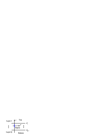
Figure 1: Schematic of a stratified structure. The cylindrical coordinates are set and the origin is always on the VED.

The model studied in this paper consists of a lossless layered structure with the stratification along the $z$ direction. It contains $Q$ layers and $Q-1$ interfaces from top to bottom, as depicted in Fig. 1. Since we concentrate on the far field, the two semispaces, i. e., the top and bottom layers, are focused on and the intermediate regions are ignored when their details are not needed. The lower surface of the top layer is at $z=d_{1}$ and the upper surface of the bottom layer is at $z=d_{Q-1}$, respectively. A vertical electric dipole (VED) is located on the origin inside the structure. For convenience, we consider the $z$ component of the electric fields $E_{z}$ generated by the VED. Other field components and other dipole orientations will be discussed in Sec. 5. In Fig. 1, the cylindrical coordinates $(\rho,\varphi,z)$ are set. If the VED is either in the top layer or in the intermediate region, the field $E_{z}$ in the top and bottom layers is expressed as r06

$$E_{z}(\rho,z)=\left\{\begin{array}[]{rcl}\displaystyle[P.F.]\delta_{1q}-\frac{\omega\mu_{0}\mu_{1}j_{z}}{8\pi k_{1}^{2}}\int_{-\infty}^{\infty}dk_{\rho}\frac{k_{\rho}^{3}}{k_{qz}}H_{0}^{(1)}(k_{\rho}\rho)[C_{1}e^{ik_{1z}(z-d_{1})}],&&{z>d_{1}.}\\ \displaystyle-\frac{\omega\mu_{0}\mu_{Q}j_{z}}{8\pi k_{Q}^{2}}\int_{-\infty}^{\infty}dk_{\rho}\frac{k_{\rho}^{3}}{k_{qz}}H_{0}^{(1)}(k_{\rho}\rho)[C_{Q}e^{-ik_{Qz}(z-d_{Q-1})}],&&{z<d_{Q-1}.}\end{array}\right.$$

The quantities in this expression are as follows. $H_{0}^{(1)}$ represents the Hankel function of the first kind; $j_{z}$ is the dipole moment in the $z$ direction; $C_{1}$ and $C_{Q}$ are respectively the scattering coefficients in the top and bottom layers; $k_{q}=\omega\sqrt{\varepsilon_{q}\mu_{q}}/c=(k_{\rho}^{2}+k_{qz}^{2})^{1/2}$ is the wave vector in the $q$th layer; $\omega$ is the angular frequency; $c$ is light speed in vacuum; $\mu_{0}$ and $\mu_{q}$ are respectively the permeability in vacuum and in the $q$th layer; $P.F.$ standing for primary field, is the $E_{z}$ generated by the VED in a homogeneous background; $\delta_{1q}$ is Kronecker delta. In Eq. (1), the VED is not allowed to appear in the bottom layer. However, if the VED is in the bottom layer, one may use the reversed geometry instead.

III 3. Bilayer structures

This section discusses the far-field asymptotic behaviors of dipole radiations and the NFFF boundary in bilayer structures.

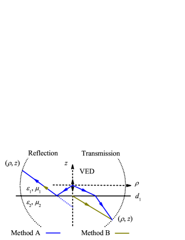
Figure 2: Physical meanings of SPs in a bilayer structure. Method A: blue lines; Method B: yellow lines. For reflections, Method A and B show the same picture that the reflected field is equal to a field generated by an image point of VED mirrored by the interface. For transmissions, Method A describes a refraction that satisfies Snell’s law, while Method B sets the start point on the interface right below the VED.

In this case, the intermediated region in Fig. 1 is removed, and the interfaces at $z=d_{1}$ and $d_{Q-1}$ merge into one, as shown by Fig. 2. The top and bottom layers are also denoted as layer 1 and 2, respectively.

III.1 3.1. The expressions of the $E_{z}$ in the far-field zones

In the case of bilayer structures shown in Fig. 2 ($d_{1}<0$), $C_{1}$ and $C_{Q}$ in Eq. (1) are expressed as

$$\left\{\begin{array}[]{rcl}\displaystyle C_{1}=r_{12}e^{-ik_{1z}d_{1}}=\frac{k_{1z}/\varepsilon_{1}-k_{2z}/\varepsilon_{2}}{k_{1z}/\varepsilon_{1}+k_{2z}/\varepsilon_{2}}e^{-ik_{1z}d_{1}},\\ \displaystyle C_{2}=t_{12}e^{-ik_{1z}d_{1}}=\frac{2k_{1z}/\varepsilon_{1}}{k_{1z}/\varepsilon_{1}+k_{2z}/\varepsilon_{2}}e^{-ik_{1z}d_{1}},\end{array}\right.$$

where $\varepsilon_{q}$ is the relative permittivity of the $q$th layer. In this paper, $r_{ij}$ and $t_{ij}$ denote the Fresnel scattering coefficients of a single interface when light incidents from layers $i$ to $j$. Here we carry out a detailed derivation on the transmission field with two asymptotic treatments. In this process, the similarities and discrepancies between these two treatments are disclosed.

Substitution of Eq. (2) into (1) and application of the asymptotic form of Hankel function give the expression of $E_{z}$ in layer 2:

$$E_{z}(z<d_{1})=-\frac{\omega\mu_{0}\mu_{2}j_{z}}{8\pi k_{2}^{2}}\int_{-\infty}^{\infty}dk_{\rho}\frac{k_{\rho}^{3}}{k_{1z}}t_{12}e^{i(k_{\rho}\rho-\pi/4)}e^{-ik_{2z}(z-d_{1})}e^{-ik_{1z}d_{1}}.$$

The SP is obtained by taking derivative of the phase as follows:

$$\rho+\frac{k_{\rho s}}{k_{1zs}}d_{1}+\frac{k_{\rho s}}{k_{2zs}}(z-d_{1})=0.$$

This way determining the SP is called Method A. Its physical meaning can be explained by ray theory. On the other hand, if the factor $\exp(-ik_{1z}d_{1})$ in Eq. (3) is a slowly varying one, it can be taken out of the integral, and the remaining phase gives the SP as follow:

$$\rho+\frac{k_{\rho s}}{k_{2zs}}(z-d_{1})=0.$$

This way is called Method B r26 ; r27 . In Eqs. (4a) and (4b), the subscript “s” stands for stationary points. Here we emphasize the features of these two methods. Method A treats $\exp(-ik_{1z}d_{1})$ as an oscillatory factor. As a result, the term $k_{\rho s}d_{1}/k_{1zs}$ is included in Eq. (4a) in determining the SP. It describes the wave paths in both layers and gives the refraction picture shown by the blue lines in Fig. 2. By contrast, Method B treats $\exp(-ik_{1z}d_{1})$ as a slowly varying one so that the term $k_{\rho s}d_{1}/k_{1zs}$ is excluded in Eq. (4b) in determining the SP. This description is merely applicable to the wave path in layer 2, as shown by the yellow lines in Fig. 2.

Under these points of view, Method A gives the electric field as

$$E_{z}(z<d_{1})=-\frac{\omega\mu_{0}\mu_{2}j_{z}}{8\pi k_{2}^{2}}t_{12}(k_{\rho s})\frac{k_{2zs}}{k_{1zs}}k_{\rho s}^{2}\int_{-\infty}^{\infty}dk_{\rho}\frac{k_{\rho}}{k_{2z}}H_{0}^{(1)}(k_{\rho}\rho)e^{-ik_{2z}(z-d_{1})-ik_{1z}d_{1}},$$

while Method B gives

$$E_{z}(z<d_{1})=-\frac{\omega\mu_{0}\mu_{2}j_{z}}{8\pi k_{2}^{2}}t_{12}(k_{\rho s})\frac{k_{2zs}}{k_{1zs}}k_{\rho s}^{2}e^{-ik_{1zs}d_{1}}\int_{-\infty}^{\infty}dk_{\rho}\frac{k_{\rho}}{k_{2z}}H_{0}^{(1)}(k_{\rho}\rho)e^{-ik_{2z}|z-d_{1}|}.$$

The simplification in Method B is that the integral in Eq. (5b) can be expressed as spherical waves using the Sommerfeld identity r06 ; r20

$$\frac{e^{ikr}}{r}=\frac{i}{2}\int_{-\infty}^{\infty}dk_{\rho}\frac{k_{\rho}}{k_{z}}H_{0}^{(1)}(k_{\rho}\rho)e^{-ik_{z}|z|}.$$

By contrast, Eq. (5a) cannot be further reduced in mathematics because its exponential term contains two different wave vectors. We have to carry out the integral according to Eq. (4a). The corresponding ray interpretation is demonstrated by blue lines in Fig. 2.

After integrations, the asymptotic expressions of $E_{z}$ in Method A and B are respectively given by

$$\left\{\begin{array}[]{rcl}E_{z}(z<d_{1})&=&\displaystyle-\frac{\omega\mu_{0}\mu_{2}j_{z}}{8\pi k_{2}^{2}}t_{12}(k_{\rho s})\frac{k_{2zs}}{k_{1zs}}k_{\rho s}^{2}\left[\frac{2}{i}\frac{e^{ik_{1}\triangle r_{1}}e^{ik_{2}\triangle r_{2}}}{\triangle r_{1}+\triangle r_{2}}\right]\\ &=&\displaystyle t_{12}(k_{\rho s})\frac{k_{2zs}}{k_{1zs}}e^{i(k_{1}-k_{2})\triangle r_{1}}\left\{\frac{i\omega\mu_{0}\mu_{2}j_{z}}{4\pi k_{2}^{2}}k_{\rho s}^{2}\frac{e^{ik_{2}(\triangle r_{1}+\triangle r_{2})}}{\triangle r_{1}+\triangle r_{2}}\right\}\\ \triangle r_{1}&=&\displaystyle\frac{k_{1}}{k_{1zs}}|d_{1}|\\ \triangle r_{2}&=&\displaystyle\frac{k_{2}}{k_{2zs}}|z-d_{1}|\end{array}\right.$$

and

$$\left\{\begin{array}[]{rcl}E_{z}(z<d_{1})&=&\displaystyle-\frac{\omega\mu_{0}\mu_{2}j_{z}}{8\pi k_{2}^{2}}t_{12}(k_{\rho s})\frac{k_{2zs}}{k_{1zs}}k_{\rho s}^{2}e^{-ik_{1zs}d_{1}}\left[\frac{2}{i}\frac{e^{ik_{2}r_{2}}}{r_{2}}\right]\\ &=&\displaystyle t_{12}(k_{\rho s})\frac{k_{2zs}}{k_{1zs}}e^{-ik_{1zs}d_{1}}\left\{\frac{i\omega\mu_{0}\mu_{2}j_{z}}{4\pi k_{2}^{2}}k_{\rho s}^{2}\frac{e^{ik_{2}r_{2}}}{r_{2}}\right\}\\ r_{2}&=&\sqrt{\rho^{2}+(z-d_{1})^{2}}\end{array}.\right.$$

The expressions in the square brackets in Eqs. (6a) and (6b) are the resultants of the integrals in Eqs. (5a) and (5b), and those in the curly brackets represent the propagations of $E_{z}$ along the blue and yellow lines shown in Fig. 2, respectively. Thus it is easy to see that Eq. (6a) considers $E_{z}$ as spherical waves in both layers and describes a refraction process at the interface. The factor $\exp[i(k_{1}-k_{2})\triangle r_{1}]$ in Eq. (6a) is the phase correction for the spherical wave propagating in layer 1, as can be seen by comparison of Eqs. (6a) and (6b). The term $t_{12}(k_{\rho s})k_{2zs}/k_{1zs}$ arises from the boundary condition.

The physical explanation of Eq. (6b) is similar. The factor $\exp(-ik_{1z}d_{1})$ reflects the influence of the wave in layer 1. In layer 1, $E_{z}$ is a plane wave propagating along the $z$ direction, and after crossing the interface at the point right below the VED, it turns to the spherical wave and propagates to the observation points.

Method B was given by Refs. r26 ; r27 . Comparatively, Method A provides a more accurate description and asymptotic expression for the transmission than Method B. That is why we suggest Method A in this paper. However, the discrepancies of these two methods tend to be trivial as $d_{1}/r$ goes to zero. Another treatment of the transmission field r22 ; r23 ; r24 employed Eqs. (4a) and (6b). In other words, it considered $\exp(-ik_{1z}d_{1})$ first as an oscillatory term to calculate the SP, and then as a slowly varying one to take out the integral. The accuracy of this method is between Method A and B. We do not discuss it in the following.

Now let us show the equivalence between the asymptotic method, Method B, and the reciprocal theorem. Eq. (6b) can be reformed as

$$E_{z}(z<d_{1})=\frac{\varepsilon_{2}}{\varepsilon_{1}}t_{21}(k_{\rho s})e^{-ik_{1zs}d_{1}}\left\{\frac{i\omega\mu_{0}\mu_{2}j_{z}}{4\pi k_{2}^{2}}k_{\rho s}^{2}\frac{e^{ik_{2}r_{2}}}{r_{2}}\right\}$$

because

$$t_{12}(k_{\rho s})\frac{k_{2zs}}{k_{1zs}}=\frac{\varepsilon_{2}}{\varepsilon_{1}}\frac{2k_{2zs}/\varepsilon_{2}}{k_{1zs}/\varepsilon_{1}+k_{2zs}/\varepsilon_{2}}=\frac{\varepsilon_{2}}{\varepsilon_{1}}t_{21}(k_{\rho s}).$$

Since $t_{21}(k_{\rho s})$ is the transmission coefficient when light incidents from layers 2 to 1, Eq. (7) describes the reversal propagation picture: the $E_{z}$ is now generated by a VED at far-field zone and propagates back alone the reversal direction of the yellow line in Fig. 2. After crossing the interface, the spherical wave turns to a plane wave and propagates to the origin. That the spherical wave emitted by a test source turns to a plane wave after passing the interface is the treatment of the reciprocal theorem. In Ref. r32 , the turning point was chosen such that it was at the line along the direction of the VED. Therefore, the result there was the same as Eq. (6b) here. The conclusion is that Method B is equivalent to the reciprocal theorem.

When the observation points and the source are in the same layer, the reflection process described by Methods A and B are identical r02 ; r03 ; r04 ; r05 ; r06 , as shown in Fig. 2. The asymptotic expression of $E_{z}$ in layer 1 is expressed as

$$\left\{\begin{array}[]{rcl}E_{z}(z>d_{1})&=&\displaystyle[P.F.]\delta_{1q}+r_{12}(k_{\rho s})\left\{\frac{i\omega\mu_{0}\mu_{1}j_{z}}{4\pi k_{1}^{2}}k_{\rho s}^{2}\frac{e^{ik_{1}r_{1}}}{r_{1}}\right\}\\ r_{1}&=&\sqrt{\rho^{2}+(z-2d_{1})^{2}}\end{array}.\right.$$

III.2 3.2. The features of the fields

With the formulas derived above, we are able to do numerical computation. The numerical results of the asymptotic methods are compared to the precise numerical ones r10 . This enables us to acquire the NFFF boundary. As an example, we take $\lambda_{0}=1.5\mu m$ and $\mu_{q}=1$. As can be seen later, our conclusions are valid for other wavelengths and permeabilities. Since $E_{z}$ is of an axial symmetry, the angular direction $\varphi$ is not considered. Instead, the observation points are labeled by the spherical coordinates $(r,\theta,\varphi)$. Figure 3 shows the value of $|E_{z}|$ as a function of angle $\theta$, at different distance $r$. When $0\leq\theta\leq\pi/2$, the observation point is in layer 1, while when $\pi/2\leq\theta\leq\pi$, the observation point is in layer 2. In Fig. 3, the dielectric constants in layers 1 and 2 are set to be 1 and 2.25, respectively. So, the upper and lower layers are called lower and higher refraction index (RI) layers, respectively.

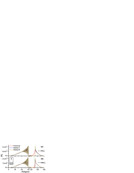
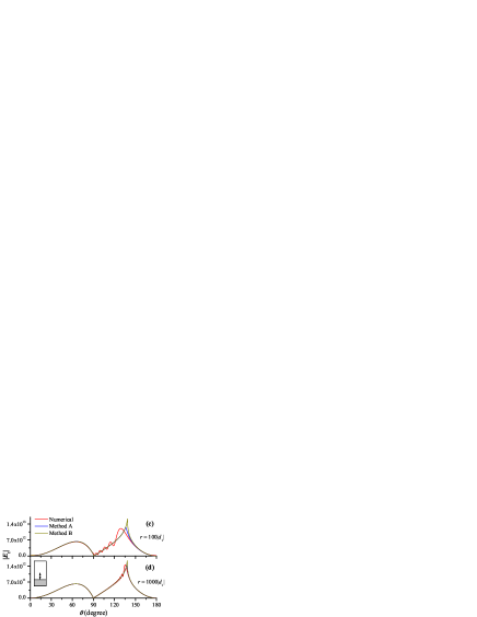
Figure 3: $|E_{z}|$ as a function of angle $\theta$ for different distance $r$. Structural schematics are illustrated in the insets. The critical angle is $\theta_{c}\sim$($180^{\circ}$–$42^{\circ}$)=$138^{\circ}$. (a) ($|d_{1}|,r$)=($10,1000$)$\lambda_{0}$. (b) ($|d_{1}|,r$)=($10,10000$)$\lambda_{0}$. (c) ($|d_{1}|,r$)=($0.1,10$)$\lambda_{0}$. (d) ($|d_{1}|,r$)=($0.1,100$)$\lambda_{0}$.

In Fig. 3, the precise numerical results r10 are plotted by red lines for comparison. For reflections, the oscillation curves in Figs. 3(a) and 3(b) reflect the interference between the primary field and reflected field, while this pattern is not shown in Figs. 3(c) and 3(d) because the distance between the VED and its image is too close. The asymptotic results fit the numerical ones very well when $r$ is of the order of $10\lambda_{0}$, or smaller $r\sim\lambda_{0}$ r23 , which agrees with the NFFF boundary in a vacuum background.

When transmitting from the lower RI layer to the higher RI one, there exists a critical angle $\theta_{c}$ above and below which are allowed and forbidden regions, respectively r36 ; r37 . The boundaries of the forbidden regions are indicated by the transmission peaks in Fig. 3. Please note that $\theta_{c}$ is related to $d_{1}$ value, so that the transmission peaks in the four panels of Fig. 3 have slight differences. In Figs. 3(c) and 3(d), the curves in the forbidden regions show ripples which is an interference effect caused by the boundary continuity r35 . Since the ripple is a near field effect, it does show up in Figs. 3(a) and 3(b) where the observation distance is far. When the distance is less, the ripple will become evident. Moreover, when the real part of $k_{1z}$ vanishes, $\exp(-ik_{1z}d_{1})$ should be treated as a slowly varying term, which means that Method A can be replaced by Method B near $\theta_{c}$ and within the forbidden region.

In the allowed region, although Method A provides more accurate results, both of them coincide with the numerical results. However, within the forbidden region and around $\theta_{c}$, there is a big difference between our results and the numerical ones. When the VED is far away from the interface, as shown in Fig. 3(a), the asymptotic result decays rapidly around $\theta_{c}$ due to the effect of $\exp(-ik_{1z}d_{1})$, while the red line shows a slow attenuation. At first glance, this seems strange since the numerical results also contain $\exp(-ik_{1z}d_{1})$. This can be answered by Eqs. (3) and (6b). The numerical method treats $\exp(-ik_{1z}d_{1})/k_{1z}$ in Eq. (3) as a whole factor, which means that when both of the numerator and denominator tend to 0, $k_{1z}$ slows down the decay of $\exp(-ik_{1z}d_{1})$. While the asymptotic methods treat $1/k_{1z}$ as a constant, implying that only the decay of $\exp(-ik_{1z}d_{1})$ is considered. In SIs, $k_{1z}=0$ corresponds to the $k_{1}$ branch point, and at this point the integration gives a lateral wave r02 ; r03 ; r04 ; r05 ; r06 . Lateral waves are the surface waves that mainly exist in the higher RI semispace and exponentially decay in the lower RI one. This explanation is also in line with the description of the steepest descent method. Near $\theta_{c}$, the steepest descent path approaches the $k_{1}$ branch point and its contribution to the integral becomes inegligible. In the forbidden region, the branch point is enclosed within the deformed integration path, and causes the lateral waves to appear in the forbidden region. Since the lateral waves represent a higher-order attenuation, it is not covered by the LOA. This indicates that the differences between the asymptotic results and numerical results come from the branch point contributions.

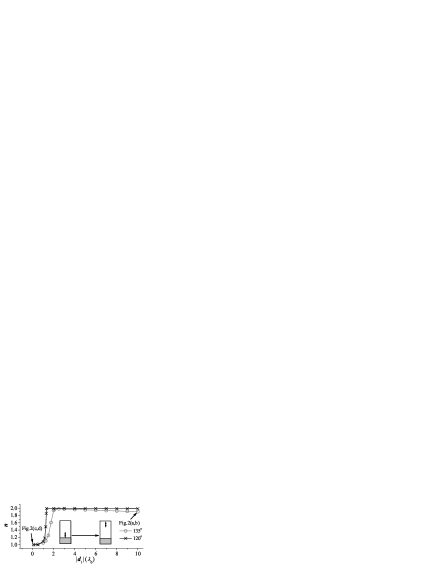
Figure 4: Results of the power series fitting the amplitude of the lateral waves at angles $120^{\circ}$ and $135^{\circ}$ in Fig. 3. Fitting functioin is $|E_{z}|$=$ar^{-n}$, where $a$ (not show here) and $n$ are fitting coefficients. The fitting range is $r$=$4000\sim 10000\lambda_{0}$ r38 .

The branch point contributions can also be treated by asymptotic methods, e. g., branch cut integrals based on the steepest descent method r29 ; r30 ; r31 , or uniform asymptotic expansions r06 . However, these methods regard $\exp(-ik_{1z}d_{1})$ as a slowly varying term r06 ; r29 ; r30 , and numerical computation is resorted r13 ; r15 ; r31 . It is difficult to generalize such asymptotic expressions to the cases of multilayer structures r30 . The exploration of asymptotic expressions for branch cut integrals is beyond the scope of this paper, so here we numerically calculate the decay behaviors of the lateral waves at angles $120^{\circ}$ and $135^{\circ}$ in Fig. 3, and show them in Fig. 4. It is seen from Fig. 4 that when $|d_{1}|>2\lambda_{0}$, the lateral waves decay as $r^{-2}$. This coincides with the case shown in Figs. 3(a) and 3(b) where $r$ decreases by one order of magnitude while the field decreases by two orders. When $\lambda_{0}<|d_{1}|<2\lambda_{0}$, the way of the decay of the lateral waves turns to $r^{-1}$, so that in Figs. 3(c) and 3(d) the numerical results and the asymptotic results have similar distributions in the forbidden region.

III.3 3.3. Determining the NFFF boundary

Having the knowledge of the decay behaviors of the lateral waves, we discuss the NFFF boundary in the bottom layer. As can be seen from Fig. 3, the boundary may be chosen as $L\sim 1000|d_{1}|$, which satisfies the evaluation of the order of magnitude indicated by Fig. 4. However, this distance should be modified because of two reasons. One is that for a very small $|d_{1}|$, e. g., $|d_{1}|=0.001\lambda_{0}$, $L\sim\lambda_{0}$ may not eliminate the influence of the lateral waves (numerically verified), which means that a lower boundary should be better. Considering Fig. 3(d), the boundary may be written as $L\sim 1000\times$Max$\{|d_{1}|,0.1\lambda_{0}\}$, where Max$\{,\}$ means “choose the larger one”. The other is that compared to the one of a homogeneous background, the NFFF boundary here has a looser relationship with $\lambda_{0}$. Although the two $|d_{1}|$ values in Fig. 3 differ by 100 times, the NFFF boundary only depends on $|d_{1}|$. Moreover, as implied by Eqs. (3), (6a) and (6b), the field distribution has a scale invariance over $\lambda_{0}$ in a non-dispersive media, indicating that the field behaviors shown in Fig. 3 stand also for other light wavelengths. So, what influences does $\lambda_{0}$ have on the NFFF boundary? Except for the lower boundary, it mainly decides the location of the forbidden region and introduces dispersion. The dispersion considered, the NFFF boundary is suggested to be

$$L\sim 1000\frac{n_{max}}{n_{min}}\times\mbox{Max}\{D,0.1\lambda_{0}\},$$

where $n_{max}$ and $n_{min}$ respectively represent the largest and smallest RI in the structure, $n_{q}=(\varepsilon_{q}\mu_{q})^{1/2}$. Equation (9) is the most significant conclusion of this paper, and it is valid for any stratified configuration, as will be illustrated below. Here, a dimensional parameter $D$ is introduced. In the present bilayer structure, $D$ equals to $|d_{1}|$. For other configurations with more layers, $D$ needs to be modified, as will be shown below.

In the following, we test Eq. (9) with other configurations. To avoid repetition, the subsequent discussion will not compare the results of different observation distances, but only focus on those at $r=100\lambda_{0}$, a distance less than that given by Eq. (9).

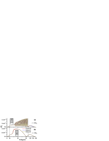
Figure 5: $|E_{z}|$ as a function of angle $\theta$ at distance $r$=$100\lambda_{0}$. Structural schematics are illustrated in the insets. The critical angle is $\theta_{c}\sim 42^{\circ}$. (a) $|d_{1}|$=$10\lambda_{0}$. (b) $|d_{1}|$=$0.1\lambda_{0}$. The coordinate between $30^{\circ}\sim 96^{\circ}$ is stretched to clearly show the oscillation details.

Now we set the dielectric constants in layers 1 and 2 to be 2.25 and 1, respectively. So, in this case the VED is in a higher RI layer. $|E_{z}|$ as a function of angle $\theta$ for two $|d_{1}|$ values is plotted in Fig. 5. In the range $0\leq\theta\leq\pi/2$, i. e., in layer 1, the oscillations shown in Figs. 5(a) and 5(b) reflect the interference between the primary and reflected fields as have been mentioned in analyzing Fig. 3. Since the lateral waves favor to appear in the higher RI semispace, in the present case, they mainly influence the reflection.

In Fig. 5, the coordinates between $30^{\circ}\sim 96^{\circ}$ are stretched to illustrate the oscillations. Around $\theta_{c}$, the asymptotic results and the numerical results have slight differences in the range $45^{\circ}\sim 50^{\circ}$, so that Eq. (9) is also applicable here. As for the transmission, since now light is from the layer with lower RI to that with higher RI, no forbidden regions appear in this configuration. Light refracts and the asymptotic results fit the numerical results quite well.

According to the discussions above, it is known that the NFFF boundary is mainly affected by the lateral waves. In the higher RI semispace, the boundary is given by Eq. (9) and much larger than the operating wavelength; while in the lower RI semispace, the boundary is about ten wavelengths. Please notice that it is not appropriate to define the NFFF boundary by distinguishing the allowed and forbidden region, because there is no forbidden region in the configurations shown in Fig. 5.

IV 4. Trilayer structures

Now we investigate the case of trilayer structure. The three layers are called the top, middle and bottom layers, or layers 1, 2 and 3, as illustrated in Fig, 6. Two cases are involved where the location of the VED is in the top and middle layers, respectively.

Before presenting numerical results, three illustrations ought to be addressed. Firstly, different from bilayer structures, there will occur in a trilayer structure three kinds of surface modes r02 ; r03 ; r04 ; r05 ; r06 ; r39 ; r40 : guided modes, proper complex modes and improper complex modes, which correspond to poles in SIs. The first two belong to normal modes that build up the point spectrum in eigenvalue problems. While the last one is commonly referred as leaky modes which violates the radiation condition and only shows up in a certain range of angle in space r39 ; r40 . The guided modes occur in the middle layer of a mode guiding configuration where the middle layer possesses the largest RI. The proper complex modes cannot propagate far from the source due to their decaying nature. Therefore, these two kinds of modes will not be touched in the following discussions. The leaky modes affect the far-field distribution and will be considered. Secondly, because there are two interfaces in this structure, light multi-reflects in the middle layer and may cause more oscillations in the far-field distribution. We will not explain all the formations of these oscillations, but focus on the ones that may affect the NFFF boundary. Moreover, the differences between Method A and B are not obvious in the previous section because $d_{1}/r$ are small, but will be magnified by the multi-reflection in the middle layer. Thirdly, there are six possible configurations of dielectric constant distribution for a trilayer structure. We merely study two of them: $[\varepsilon:1-2.25-12]$ and $[\varepsilon:2.25-12-1]$, which are often encountered in experiments. Our conclusions are easily extended to other configurations.

IV.1 4.1. The VED is in the top layer

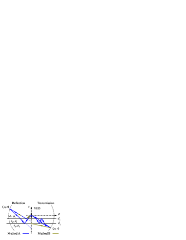
Figure 6: Physical meanings of SPs when a VED is located in the top layer. Method A: blue lines; Method B: yellow lines. Concerning reflections, Method A shows that the multi-reflection process in the middle layer contributes to the reflection in layer 1, while Method B only considers the direct reflection from the interface at $d_{1}$. For transmissions, Method A shows that the multi-reflection process contributes to the transmission in layer 3, while Method B sets the start point on the interface at $d_{2}$ right below the VED. In the figure, only the modes $m$=0 and 1 in the multi-reflection are depicted.

When the VED is in the top layer, as shown in Fig. 6 ($d_{2}<d_{1}<0$), the scattering coefficients $C_{1}$ and $C_{Q}$ are expressed as

$$\left\{\begin{array}[]{lcl}\displaystyle C_{1}=r_{12}+\frac{t_{12}r_{23}t_{21}e^{2ik_{2z}(d_{1}-d_{2})}}{1-r_{21}r_{23}e^{2ik_{2z}(d_{1}-d_{2})}}e^{-ik_{1z}d_{1}},\\ \displaystyle C_{3}=\frac{t_{12}t_{23}e^{2ik_{2z}(d_{1}-d_{2})}}{1-r_{21}r_{23}e^{2ik_{2z}(d_{1}-d_{2})}}e^{-ik_{1z}d_{1}},\end{array}\right.$$

where the expressions of the coefficients $r_{ij}$ and $t_{ij}$ can be found in Eq. (2). After expanding Eq. (10) with the geometrical optics series and following the steps in Sec. 3, the SPs of Method A for reflections can be obtained by,

$$\rho-\frac{k_{\rho s}^{(m)}}{k_{1zs}^{(m)}}(z-2d_{1})-\frac{k_{\rho s}^{(m)}}{k_{2zs}^{(m)}}2m(d_{1}-d_{2})=0,$$

where $m\in[0,\infty)$ is the order of the geometrical optics series. The SP of Method B is obtained by letting $m=0$ in Eq. (11). In the same way, the SPs of Method A for transmissions meet

$$\rho+\frac{k_{\rho s}^{(m)}}{k_{1zs}^{(m)}}d_{1}-\frac{k_{\rho s}^{(m)}}{k_{2zs}^{(m)}}(2m+1)(d_{1}-d_{2})+\frac{k_{\rho s}^{(m)}}{k_{3zs}^{(m)}}(z-d_{2})=0.$$

Since Method B only consider the phase variations in the observation layer, its transmission SP has the same form as Eq. (4b), with $d_{1}$ and $k_{2zs}$ being replaced by $d_{2}$ and $k_{3zs}$ respectively. The physical meanings of the SPs are depicted in Fig. 6. Method A describes a multi-reflection process, so that its $E_{z}$ expressions for reflections and transmissions are in the form of series expansions. Each term of the expressions is similar to Eq. (6a), where $\triangle r_{2}$ now represents the multi-reflection path in the middle layer and it is also needed for describing the path in layer 3. As for Method B, the asymptotic expressions are similar to Eqs. (6b) and (8). Moreover, the equivalence between the expressions of Method B and reciprocal theorem can also be proven, in a similar way to that done in Eq. (7).

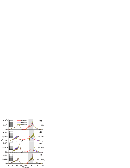
Figure 7: $|E_{z}|$ as a function of angle $\theta$ for four geometry configurations with [$\varepsilon:1-2.25-12$]. Two critical angles are $\theta_{c1}\sim$($180^{\circ}-17^{\circ}$)=$163^{\circ}$ and $\theta_{c2}\sim$($180^{\circ}-26^{\circ}$)=$154^{\circ}$. Structural schematics are illustrated in the insets. (a) ($|d_{1}|,|d_{2}|,r$)=($0.1,1.1,100$)$\lambda_{0}$. (b) ($|d_{1}|,|d_{2}|,r$)=($0.1,10.1,100$)$\lambda_{0}$. (c) ($|d_{1}|,|d_{2}|,r$)=($1.1,10.1,100$)$\lambda_{0}$. (d) ($|d_{1}|,|d_{2}|,r$)=($0.1,10.1,35000$)$\lambda_{0}$. The shaded areas between $\theta_{c1}$ and $\theta_{c2}$ are the second total internal reflection regions.

Figure 7 plots the $E_{z}$ distributions in the case of $[\varepsilon:1-2.25-12]$ configuration. Since layers 2 and 3 have higher RI, there are two critical angles: $\theta_{c1}\sim\pi-asin(1/\sqrt{12})$ and $\theta_{c1}\sim\pi-asin(1/\sqrt{2.25})$. $\theta_{c1}$ determines the forbidden region. The range between $\theta_{c1}$ and $\theta_{c2}$ is shaded in Fig. 7 and is termed as the second total internal reflection region.

In Fig. 7(a), the thickness of the middle layer is $\lambda_{0}$. It is seen that the differences between the asymptotic results and numerical results emerge in the transmission field. These differences are caused by the lateral waves as well. The dimensional parameter $D$ in Eq. (9) now should equal to the distance between VED and the lower interface at $z=d_{2}$. The calculated NFFF boundary is approximately 35 times of the observation distance, which is enough to eliminate the influence of lateral waves (numerical verified, not show here).

In Fig. 7(b), the middle layer is thicker: its thickness is $10\lambda_{0}$. This figure shows two significant features. One is that Method A and B have noticeable differences in both of the reflections and transmissions. Because Method A takes into account the multi-reflection, its results are closer to the numerical ones. The other is that in the second total internal reflection region, the asymptotic curve shows rapid oscillation [The coefficients $C_{1}$ and $C_{3}$ in Eq. (10) are of the form of multi-reflection, and in this sense, there is also multi-reflection in Method B]. The formation of the oscillation can be explained as following: although the light decays in the top layer, part of the energy can be transferred into the middle layer through evanescent waves and become propagation ones. Then in the middle layer it scatters at the lower boundary, and has a total internal reflection at upper boundary, which further forms a multi-reflection to yield the oscillation. When the VED moves away from the interface, the oscillation will die away. This is verified by Fig. 7(c) where $|d_{1}|$ changes from $0.1\lambda_{0}$ to $\lambda_{0}$. It is seen from Fig. 7(c) that the oscillations disappear and the far-field distribution decreases. It is worth mentioning that the description here is the picture of leaky waves. A comparatively thicker middle layer allows many leaky modes to exist, resulting in the rapid oscillation in the far-field distribution. As a test of the NFFF boundary, Fig. 7(d) plots the field distribution of the same configuration in Fig. 7(b) but with the observation point being at the NFFF boundary, i. e., with the observation distance computed by Eq. (9). The results fit each other very well.

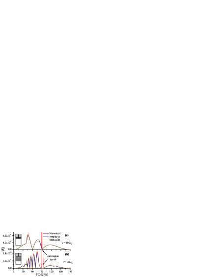
Figure 8: $|E_{z}|$ as a function of angle $\theta$ at distance $r$=$100\lambda_{0}$ for two geometry configurations with [$\varepsilon:2.25-12-1$]. The two critical angles are $\theta_{c1}\sim 26^{\circ}$ and $\theta_{c2}\sim 42^{\circ}$. Structural schematics are illustrated in the insets. $|d_{1}|$=$0.1\lambda_{0}$. (a) $|d_{2}|$=$1.1\lambda_{0}$. (b) $|d_{2}|$=$10.1\lambda_{0}$. The fields in the middle layer are not presented.

Fig. 8 shows the $|E_{z}|$ distributions in $[\varepsilon:2.25-12-1]$ configuration. Since the middle layer possesses the largest RI, the structure supports the guided modes. The peaks around $90^{\circ}$ of the numerical results are the decays of the guide modes in layers 1 and 3. Moreover, there is no forbidden region in the structure. Consequently, the asymptotic result and the numerical results fit very well. For reflections, these two kinds of results show some differences around $\theta_{c2}$ due to the effect of lateral waves, but they fit each other at the NFFF boundary given by Eq. (9). Around $90^{\circ}$, the guide modes decay in the lower RI layers, but they are not covered in the discussion here because a guided mode is a bounded state that is equivalence to cylindrical wave and have a decay rate as $1/\sqrt{\rho}$, which means that its field is much larger than the results of LOA .

IV.2 4.2. The VED is in the middle layer

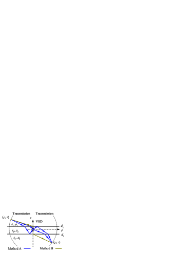
Figure 9: Physical meanings of SPs when a VED is located in the middle layer. Method A: blue lines; Method B: yellow lines. For transmissions in the top layer, two cases, both involving multi-reflection processes, are distinguished in Method A, where the propagation direction of the light is upward or downward after emitted from the VED. For a clear illustration, only the mode $m$=0 is demonstrated here. Method B sets the start point on the top interface right above the dipole. The transmissions in the bottom layer are similar to that in the top layer, but with the transmission direction reversed.

Next, we discuss the case when the VED is located in the middle layer ($d_{2}<0<d_{1}$), as shown in Fig. 9. For this configuration, the scattering coefficients $C_{1}$ and $C_{Q}$ are expressed as

$$\left\{\begin{array}[]{lcl}\displaystyle C_{1}=t_{21}\frac{e^{ik_{2z}d_{1}}}{1-r_{21}r_{23}e^{2ik_{2z}(d_{1}-d_{2})}}+t_{21}\frac{r_{23}e^{ik_{2z}(d_{1}-2d_{2})}}{1-r_{21}r_{23}e^{2ik_{2z}(d_{1}-d_{2})}},\\ \displaystyle C_{3}=t_{23}\frac{e^{-ik_{1z}d_{2}}}{1-r_{21}r_{23}e^{2ik_{2z}(d_{1}-d_{2})}}+t_{23}\frac{r_{21}e^{ik_{2z}(2d_{1}-d_{2})}}{1-r_{21}r_{23}e^{2ik_{2z}(d_{1}-d_{2})}}.\end{array}\right.$$

For the $|E_{z}|$ in the top layer, Method A expands the two terms in $C_{1}$ using geometric optics series, which is then substituted in Eq. (1) to get the SPs:

$$\left\{\begin{array}[]{lcl}\displaystyle\rho-\frac{k_{\rho s}^{(m)}}{k_{1zs}^{(m)}}(z-d_{1})-\frac{k_{\rho s}^{(m)}}{k_{2zs}^{(m)}}[2m(d_{1}-d_{2})+d_{1}]=0,\\ \displaystyle\rho-\frac{k_{\rho s}^{(m)}}{k_{1zs}^{(m)}}(z-d_{1})-\frac{k_{\rho s}^{(m)}}{k_{2zs}^{(m)}}[2(m+1)(d_{1}-d_{2})-d_{2}]=0.\end{array}\right.$$

On the whole, Eq. (14) represents the light transmitting to the top layer after multi-reflections. The first equation represents the case of light propagating upward after being emitted from the VED. The second equation indicates the fact that light propagates downwards first, and after is reflected by the lower interface, it then propagates upwards. The intuitive picture is illustrated in Fig. 9. This course is also reflected by the expression of $C_{1}$ in Eq. (13). Concerning the ray interpretation of SPs, we can write the asymptotic expressions similar to Eq. (6a). The transmission picture of Method B is the same as the above ones, and its asymptotic expressions are similar to Eq. (6b). The transmission to the bottom layer is similar to that to the top layer, but with the direction in reverse.

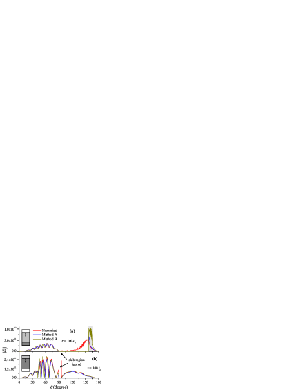
Figure 10: $|E_{z}|$ as a function of angle $\theta$ at distance $r$=$100\lambda_{0}$ for two configurations. The two critical angles are $\theta_{c1}\sim$($180^{\circ}-17^{\circ}$)=$163^{\circ}$ and $\theta_{c1}\sim$($180^{\circ}-26^{\circ}$)=$154^{\circ}$. Structural schematics are illustrated in the insets. ($|d_{1}|,|d_{2}|,r$)=($0.1,10,100)\lambda_{0}$. (a) [$\varepsilon:1-2.25-12$]. (b) [$\varepsilon:2.25-12-1$]. The gray area in (a) represents the second total internal reflection region.

The $|E_{z}|$ distributions when the VED is in the middle layer of trilayer structures are shown in Fig. 10. Figures 10(a) and 7(b) have similar far-field distributions, and Figs. 10(b) and 8(b) as well. Therefore, the discussions there are valid for Fig. 10. The correctness of Eq. (9) is again verified, where the parameter $D$ is now the thickness of the middle layer. Moreover, Fig. 10 also shows that Method A provides more accurate results than Method B.

It is known from the discussions above that conclusions about the NFFF boundary in a trilayer structure are similar to that obtained in a bilayer structure. The boundary in a higher RI layer is mainly determined by the lateral waves and satisfies Eq. (9), while the boundary in the lowest RI layer is about ten wavelengths.

V 5. General configurations

In this section, we generalize our conclusions to multilayer structures, and verify the universality of Eq. (9).

For multilayer structures, light multi-reflects in each layer in the intermediate region. Consequently, the expressions of the field will have a recursive fashion, which will make the ray interpretations very complicated and limit the applicability of Method A. However, Method B is still of the simplicity in mathematics and is suitable for multilayered structures.

The NFFF boundary in the multilayered structures is mainly affected by the lateral waves as well. The attenuation behaviors of these waves are similar to the ones shown in Fig. 4, so that Eq. (9) is correct in the order of magnitude. The value of the dimensional parameter $D$ depends on whether the VED is in the top layer or in the intermediated region. When the VED is in the top layer, $D$ equals the distance between the VED and the lowest interface at $z=d_{Q-1}$; when the VED is in one of the intermediate layer, $D$ is the distance between the highest interface at $z=d_{1}$ and lowest interface at $z=d_{Q-1}$, which is the total thickness of the intermediate region. The multi-reflection processes do not affect the $D$ value for the following two reasons. Firstly, the multi-reflections have a quick convergence. All the results of Method A shown in the figures converge when $m$ is up to $2\sim 4$, which does not change the order of $D$. Secondly, as can be seen from Fig. 4, the lateral waves have a nearly $r^{-1}$ decay when $D$ is small, and have a more rapid decay when $D$ is relatively larger. Therefore the influence from the multi-reflection may decay to a negligible one within the distance given by Eq. (9). Moreover, it is this decay characteristic of the lateral waves that makes the NFFF boundary almost independent of the wavelength.

For other field components of the dipole radiations and the cases of different dipole orientations, we have numerically verified the correctness of Eq. (9). Besides, all these cases depend on the evaluations of the scattering coefficients related SIs, but the field expressions are slightly different, which results in different far-field patterns over the observation angles. However, in the asymptotic analysis, they have the same SPs and similar asymptotic expressions and branch cut contributions. Thus, Eq. (9) is applicable.

In the beginning of Sec. 2, we have assumed that all of the layers were lossless. Now let us discuss what about the case where the intermediate region is not lossless. In such a situation, two cases are distinguished to discuss the NFFF boundary: the loss is large or small. When the loss is large, as in undersea communications where short waves may not reach the sea bottom r22 ; r23 ; r24 , the air-ocean-earth trilayer model simplifies to an air-ocean bilayer one. From the discussions in Sec. 3, a distance of $10\lambda_{0}$ is enough to differentiate the near field and far field in air. When the loss is relatively small, the amplitude of light decreases as it arrives the bottom interface, which accordingly leads to a decrease of the differences between the asymptotic results and the accurate ones. Generally speaking, losses make the NFFF boundary reduced: its value will be less than that given by Eq. (9).

Our conclusion can extend to bulk sources. On the one hand, within the scope of volume integral method r08 , a bulk source can be considered as a superposition of dipoles. The far-field radiations of each dipole have been fully discussed above. On the other hand, within the scope of NFFF transformation r07 ; r27 ; r28 , the near fields of an arbitrary source can be converted to equivalence surface dipoles on a virtual closed surface. Therefore the dimensional parameter $D$ should anchor to the brightest spots in the near field. Of course, our conclusions can be considered as an applicable scope of the NFFF transformation.

VI 6. Concluding remarks

In this paper, we have investigated the far-field asymptotic behaviors of dipole radiations in stratified backgrounds and obtain a universal empirical expression of NFFF boundary, Eq. (9). The asymptotic results are compared with the accurate numerical ones in various configurations to make sure the universality of Eq. (9). The NFFF boundary is mainly affected by the lateral waves, which correspond to branch point contributions in the SIs and are of a higher-order attenuation. In Eq. (9), the parameter $D$ plays a key role, and it is much larger than the operating wavelength. As a result, the NFFF boundary in a stratified background is totally different from that in vacuum. To be more specific, Eq. (9) describes the boundary between the intermediate and far fields. However, since the intermediate field is vaguely defined in optics, we still call it as the NFFF boundary. In the case that the observation point is in a region where its RI is the lowest in the whole structure (usually air), the lateral wave decay rapidly, and the NFFF boundary is about ten wavelengths.

It is believed that our conclusions are very helpful in understanding and applying the far-field approximation. In electromagnetic simulations, such as the finite-difference time-domain method and the finite element method, the far-field results are obtained by a NFFF transformation where the far field approximation, or the LOA, is employed. The NFFF boundary presented here reveals the applicability of the NFFF transformation, especially in the forbidden region. Moreover, we compare the different treatments for SPs in the asymptotic method and improve the accuracy according to the ray theory (Method A). The equivalence between the results of the asymptotic method and reciprocal theorem is demonstrated.

References

- (1)
- (2) [†] E–mail: wangxueh@mail.sysu.edu.cn
- (3) B. Keiser, Principles of Electromagnetic Compatibility (Artech House, 1987).
- (4) M. Born and E. Wolf, Principles of Optics (Cambridge University Press, 1999).
- (5) J. A. Kong, Electromagnetic Wave Theory (Wiley Interscience, 1986).
- (6) J. R. Wait, Electromagnetic Waves in Stratified Media (Pergamon, 1970).
- (7) J. R. Wait, Geo-electromagnetism (Academic Press, 1982).
- (8) W. C. Chew, Waves and Fields in Inhomogeneous Media (Van Nostrand Reinhold, 1990).
- (9) A. Taflove, Computational Electrodynamics: The Finite-Difference Time-Domain Method (Artech House, 1995).
- (10) W. C. Chew, J. M. Jin, E. Michielssen, and J. Song, Fast and Efficient Algorithms in Computational Electromagnetics (Artech House, 2001).
- (11) W. C. Chew and L. J. Jiang, “Overview of large-scale computing: The past, the present, and the future,” Proc. IEEE 101(2), 227–241 (2013).
- (12) M. Paulus, P. Gay-Balmaz, and O. J. F. Martin, “Accurate and efficient computation of the Green’s tensor for stratified media,” Phys. Rev. E62(4), 5797–5807 (2000).
- (13) Y. L. Chow, J. J. Yang, D. G. Fang, and G. E. Howard, “A closed form spatial Green’s function for the thick microstrip substrate,” IEEE Trans. Microwave Theory Tech. 39(3), 588–592 (1991).
- (14) R. R. Biox, A. L. Fructos, and F. Medina, “Closed-form uniform asymptotic expansions of Green’s functions in layered media,” IEEE Trans. Antennas Propag. 58(9), 2934–2945 (2010).
- (15) Y. P. Chen, W. C. Chew, and L. Jiang, “A novel implementation of discrete complex image method for layered medium Green’s function,” IEEE Antennas Wireless Propag. Lett. 10, 419–422 (2011).
- (16) D. G. Kurup, “Spatial domain Green’s functions of layered media using a new method for Sommerfeld Integrals,” IEEE Microw. Wireless Compon. Lett. 22(4), 161–163 (2012).
- (17) F. Mesa, R. R. Biox, and F. Medina, “Closed-form expressions of multilayered planar Green’s functions that account for the continuous spectrum in the far field,” IEEE Trans. Microwave Theory Tech. 56(7), 1601–1614 (2008).
- (18) T. Kaifas, “Direct rational function fitting method for accurate evaluation of Sommerfeld integrals in stratified media,” IEEE Trans. Antennas Propag. 60(1), 282–291 (2012).
- (19) M. Abramowitz and I. A. Stegun, Handbook of Mathematical Functions (Dover, 1972).
- (20) N. Bleistein and R. A. Handelsman, Asymptotic Expansions of Integrals (Holt, Rinehart, and Winston, 1975).
- (21) C. Bender and S. Orzag, Advanced Mathematical Methods for Scientists and Engineers (McGraw-Hill, 1978).
- (22) W. C. Chew, “A quick way to approximate a Sommerfeld-Weyl-type integral [antenna far-field radiation],” IEEE Trans. Antennas Propag. 36(11), 1654–1657 (1988).
- (23) Y. L. Long and H. Y. Jiang, “Error analysis for far-field approximate expression of sommerfeld-type integral,” IEEE Trans. Antennas Propag. 42(4), 574 (1994).
- (24) Y. L. Long , H. Jiang, and B. Rembold, “Far-region electromagnetic radiation with a vertical magnetic dipole in sea,” IEEE Trans. Antennas Propag. 49(6), 992–996 (2001).
- (25) Z. J. Liu and L. Carin, “Efficient evaluation of the half-space Green’s function for fast-multipole scattering models,” Microw. Opt. Technol. Lett. 29(6), 388–392 (2001).
- (26) O. M. Abo-Seida , S. T. Bishay, and K. M. El-Morabie, “Far-field radiated from a vertical magnetic dipole in the sea with a rough upper surface,” IEEE Trans. Geosci. Remote Sens. 44(8), 2135–2142 (2006).
- (27) G. P. Otto, C. Lu, and W. C. Chew, “Circular short backfire antenna modeling,” IEEE Trans. Antennas Propag. 40(11), 1434–1438 (1992).
- (28) K. A. Michalski and D. Zheng, “Analysis of microstrip resonators of arbitrary shape,” IEEE Trans. Microwave Theory Tech. 40(1), 112–119 (1992).
- (29) I. R. Capoglu, A. Taflove, and V. Backman, “A frequency-domain near-field-to-far-field transform for planar layered media,” IEEE Trans. Antennas Propag. 60(4), 1878–1885 (2012).
- (30) J. Muller, G. Parent, G. Jeandel, and D. Lacroix, “Finite-difference time-domain and near-field-to-far-field transformation in the spectral domain: application to scattering objects with complex shapes in the vicinity of a semi-infinite dielectric medium,” J. Opt. Soc. Am. A28(5), 868–878 (2011).
- (31) M. A. Marin, S. Barkeshli, and P. H. Pathak, “Efficient analysis of planar microstrip geometries using a closed-form asymptotic representation of the grounded dielectric slab Green’s function,” IEEE Trans. Microwave Theory Tech. 37(4), 669–679 (1989).
- (32) M. A. Marin and P. H. Pathak, “An asymptotic closed-form representation for the grounded double-layer surface Green’s function,” IEEE Trans. Antennas Propag. 40(11), 1357–1366 (1992).
- (33) J. R. Mosig and A. A. Melcon, “Green’s functions in lossy layered media: Integration along the imaginary axis and asymptotic behavior,” IEEE Trans. Antennas Propag. 51(12), 3200–3208 (2003).
- (34) K. Demarest, Z. Huang, and R. Plumb, “An FDTD near- to far-zone transformation for scatterers buried in stratified grounds,” IEEE Trans. Antennas Propag. 44(8), 1150–1156 (1996).
- (35) J. Y. Courtois, J. M. Courty, and J. C. Mertz, “Internal dynamics of multilevel atoms near a vacuum-dielectric interface,” Phys. Rev. A53(3), 1862–1878 (1996).
- (36) L. Cao and B. Wei, “Scattering of targets over layered half space using a semi-analytic method in conjunction with FDTD algorithm,” Opt. Express 22(17), 20691–20704 (2014).
- (37) L. Luan, P. R. Sievert, and J. B. Ketterson, “Near-field and far-field electric dipole radiation in the vicinity of a planar dielectric half space,” New J. Phys. 8(11), 264 (2006).
- (38) L. Novotny, “Allowed and forbidden light in near-field optics. I. A single dipolar light source,” J. Opt. Soc. Am. A14(1), 91–104 (1997).
- (39) H. F. Arnoldus and J. T. Foley, “Transmission of dipole radiation through interfaces and the phenomenon of anti-critical angles,” J. Opt. Soc. Am. A21(6), 1109–1117 (2004).
- (40) Since the power series could not properly retrieve the lateral wave in the vicinity of the interface, the fitting range is which is sufficiently wide for accurate fitting.
- (41) T. Tamir and A. A. Oliner, “Guided Complex Waves, Part 1: Fields at an interface,” Proc. Inst. Electr. Eng. 110(2), 310–324 (1963).
- (42) T. Tamir and A. A. Oliner, “Guided Complex Waves, Part 2: Relation to radiation patterns,” Proc. Inst. Electr. Eng. 110(2), 325–334 (1963).