Rho meson form factors in a confining Nambu–Jona-Lasinio model

Abstract

Elastic electromagnetic form factors for the $\rho^{+}$ meson are calculated in a Nambu–Jona-Lasinio model which incorporates quark confinement through the use of the proper-time regularization scheme. A comparison is made with recent lattice QCD results and previous quark model calculations for static quantities and the Sachs form factors. The results are qualitatively in good agreement with the lattice QCD calculations, with the exception of the quadrupole moment and corresponding form factor, which may be related to a lack of spherical symmetry on the lattice.

I Introduction

The structure of hadrons presents a remarkable challenge to the theory of strong interactions – quantum chromodynamics (QCD) – and a critical feature of a hadron’s structure is its distribution of charge and magnetization, which is empirically related to its electromagnetic form factors Thomas and Weise . The direct calculation of hadron form factors using QCD is currently only possible through lattice QCD, albeit limited to the low to moderate $Q^{2}$ region. However, to gain insight into the relevant dynamical mechanisms behind the observed structure it is useful to work with models that approximate key features of QCD. An important focus for this comparison are the meson form factors. Because of their short lifetimes Olive et al. (2014) they present a unique challenge experimentally – making both lattice QCD and model calculations critical. The pion form factor has been successfully measured over a wide range of four momentum transfer, while the vector meson form factors have not had the same amount of experimental exploration. However, the BABAR collaboration has measured the cross-section for the reaction $e^{+}+e^{-}\to\rho^{+}+\rho^{-}$ Aubert et al. (2008), which has been analyzed to garner information on the $\rho$-meson form factors Dbeyssi et al. (2012).

The $\rho$ form factors, or equivalently the polarization amplitudes, have been calculated using a variety of methods, for example, phenomenological models Adamuscin et al. (2007); García Gudiño and Toledo Sánchez (2014), constituent quark models in the light front framework Chung et al. (1988); Cardarelli et al. (1995); de Melo and Frederico (1997); Choi and Ji (1999); Melikhov and Simula (2002); Jaus (2003); Choi and Ji (2004); Biernat and Schweiger (2014), QCD sum rules Aliev et al. (2003); Samsonov (2003); Braguta and Onishchenko (2004); Aliev and Savci (2004) and the Dyson-Schwinger equations Hawes and Pichowsky (1999); Bhagwat and Maris (2008); Roberts et al. (2011); Pitschmann et al. (2013). The first attempts to compute $\rho$ form factors using lattice QCD were reported in Refs. Andersen and Wilcox (1997); Hedditch et al. (2007) in the quenched framework. The recent work of Owen et al. Owen et al. (2015) and Shultz et al. Shultz et al. (2015) give two independent lattice QCD calculations based upon different approaches. These lattice results, and the previous work with quark models, provides a solid background for comparison with results computed within other models.

In this work we extend the $\rho$-meson form factor calculation of Ref. Cloët et al. (2014), where the focus was a comparison with the axialvector diquark form factors which formed a critical part of a nucleon form factor calculation. Here we use the same confining version of the Nambu–Jona-Lasinio (NJL) model Nambu and Jona-Lasinio (1961a, b) to investigate the quark mass dependence of the $\rho$ form factors, and perform a detailed comparison with the lattice QCD results of Refs. Owen et al. (2015); Shultz et al. (2015). Following Ref. Cloët et al. (2014) we include the dressing of the quark-photon vertex from the inhomogenerous Bethe-Salpeter equation and a pion cloud, which are critical for a good agreement with lattice results. Similar finding were made in Ref. Ninomiya et al. (2015), where the same framework was applied to the $\pi$ and $K$ form factors.

The outline of the paper is as follows: In Sec. II we briefly review the NJL model as applied to $\bar{q}q$ bound states and the calculation of the $\rho$ electromagnetic form factors is discussed in Sec. III. The results are compared to those from lattice QCD and various quark models in Sec. IV and Sec. V presents our conclusions.

II Nambu–Jona-Lasinio Model

In its original formulation the NJL model successfully encapsulated the effects of dynamical chiral symmetry breaking, where the pion emerged as a Goldstone boson and the nucleon was the fundamental degree of freedom Nambu and Jona-Lasinio (1961a, b). The NJL model has subsequently been re-expressed with quarks as the fundamental constituents, making the relation with QCD evident. Importantly, the NJL model Klevansky (1992) preserves the fundamental symmetries of QCD. In particular, the generation of mass through the dynamical breaking of chiral symmetry is beautifully illustrated. In contrast, quark confinement is not automatically incorporated in the model. However, it has been shown that it can be mimicked by the introduction of an infrared cutoff in the proper-time regularization scheme Ebert et al. (1996); Hellstern et al. (1997); Bentz and Thomas (2001). The NJL model has a history of success in the description of numerous meson Klevansky (1992); Hatsuda and Kunihiro (1994); Vogl and Weise (1991) and baryon Hatsuda and Kunihiro (1994); Vogl and Weise (1991) properties, including the nucleon parton distribution functions Cloët et al. (2005a, b, 2008); Bentz et al. (2008); Matevosyan et al. (2012) and electromagnetic form factors Cloët et al. (2014). More recently these studies have been extended to the computation of the axial charges for strangeness conserved $\beta$-decays in the baryon octet Carrillo-Serrano et al. (2014) and possible insights into the solutions of long time enigmas in QCD, such as the $\Delta I=1/2$ rule in kaon decays Liu et al. (2015). It is this wealth of achievement, together with the recent developments in lattice QCD that encourage us to test whether the model gives an accurate description of $\rho$-meson properties.

In the application of the NJL model to the solution of the form factors of the $\rho$-meson, we use a two-flavor NJL Lagrangian which in the $\bar{q}q$ interaction channel reads:

$$\mathop{\mathcal{L}} =\bar{\psi}\left(i\not{\partial}-\hat{m}\right)\psi$$

$$+\tfrac{1}{2}\,G_{\pi}\left[\left(\bar{\psi}\psi\right)^{2}-\left(\bar{\psi}\gamma_{5}\vec{\tau}\psi\right)^{2}\right]-\tfrac{1}{2}\,G_{\omega}\left(\bar{\psi}\gamma^{\mu}\psi\right)^{2}$$

$$-\tfrac{1}{2}\,G_{\rho}\left[\left(\bar{\psi}\gamma^{\mu}\vec{\tau}\psi\right)+\left(\bar{\psi}\gamma^{\mu}\gamma_{5}\vec{\tau}\psi\right)^{2}\right],$$ (1)

where $\vec{\tau}$ are the Pauli matrices representing isospin and $\hat{m}=\text{diag}\left[m_{u},\,m_{d}\right]$ is the current quark mass matrix. We assume $m_{u}=m_{d}=m$. The fermion coupling $G_{\pi}$ represents the strength of the scalar ($\bar{q}q$) and pseudoscalar ($\bar{q}\gamma_{5}q$) interaction channels and is responsible for the dynamical generation of the dressed quark masses through the breaking of chiral symmetry. The strength of the vector-isoscalar and vector-isovector four fermion interactions is given by $G_{\omega}$ and $G_{\rho}$, respectively. The explicit breaking of $U(1)$ axial symmetry is often modeled by the inclusion of an extra six-fermion determinant interaction term, which describes the $\eta$ and $\eta^{\prime}$ mass splitting Klevansky (1992), however, this is not directly related to our calculation so we do not consider it. We regularize the NJL interaction through the proper-time regularization scheme, using an infrared cutoff ($\Lambda_{IR}$) to remove unphysical decay thresholds for hadrons into quarks Ebert et al. (1996); Hellstern et al. (1997); Bentz and Thomas (2001).

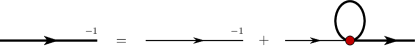
Figure 1: (Colour online) The NJL gap equation in the Hartree-Fock approximation, where the thin line represents the elementary quark propagator, $S_{0}^{-1}(k)=\not{k}-m+i\varepsilon$, and the shaded circle represents the 4-fermion interaction.

The dressed quark masses are given by the solution of the gap equation depicted in Fig. 1, which in the proper-time scheme reads

$$M=m+\frac{3}{\pi^{2}}\,M\,G_{\pi}\int_{1/\Lambda_{UV}^{2}}^{1/\Lambda_{IR}^{2}}d\tau\,\frac{e^{-\tau M^{2}}}{\tau^{2}},$$ (2)

giving a dressed quark propagator of the form:

$$S(k)^{-1}=\not{k}-M+i\varepsilon.$$ (3)

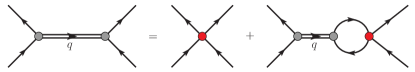
Figure 2: (Colour online) Bethe-Salpeter equation for antiquark–quark (meson) correlations in the NJL model using the random phase approximation.

The description of mesons as $\bar{q}q$ bound states in the NJL model is obtained via the Bethe-Salpeter equation (BSE) in the random-phase approximation, as illustrated in Fig. 2. The solution of the BSE in each meson channel is given by a two-body $t$-matrix that depends on the nature of the interaction channel Cloët et al. (2014), where the reduced $t$-matrices for the $\pi$, $\rho$ and $\omega$ mesons read

$$\tau_{\pi}(q) =\frac{-2i\,G_{\pi}}{1+2\,G_{\pi}\,\Pi_{PP}(q^{2})},$$ (4)

$$\tau^{\mu\nu}_{\rho(\omega)}(q) =\frac{-2i\,G_{\rho(\omega)}}{1+2\,G_{\rho(\omega)}\,\Pi_{VV}(q^{2})}$$

$$\hskip 36.98857pt\times\left[g^{\mu\nu}+2\,G_{\rho(\omega)}\,\Pi_{VV}(q^{2})\,\frac{q^{\mu}q^{\nu}}{q^{2}}\right],$$ (5)

and the bubble diagrams are defined by

$$\Pi_{PP}\left(q^{2}\right)=6i\int\frac{d^{4}k}{(2\pi)^{4}}\ \mathrm{Tr}_{D}\left[\gamma_{5}\,S(k)\,\gamma_{5}\,S(k+q)\right],$$ (6)

$$\Pi_{VV}(q^{2})\left(g^{\mu\nu}-\frac{q^{\mu}q^{\nu}}{q^{2}}\right)=$$

$$\hskip 48.36967pt6i\int\frac{d^{4}k}{(2\pi)^{4}}\ \mathrm{Tr}_{D}\left[\gamma^{\mu}\,S(k)\,\gamma^{\nu}\,S(k+q)\right].$$ (7)

The meson masses are given by the poles in the reduced $t$-matrices, that is

$$1+2\,G_{\pi}\,\Pi_{PP}\bigl{(}q^{2}=m_{\pi}^{2}\bigr{)} =0,$$ (8)

$$1+2\,G_{\rho}\,\Pi_{VV}\bigl{(}q^{2}=m_{\rho}^{2}\bigr{)} =0,$$ (9)

$$1+2\,G_{\omega}\,\Pi_{VV}\bigl{(}q^{2}=m_{\omega}^{2}\bigr{)} =0.$$ (10)

Expanding the full $t$-matrices about these poles gives the homogeneous Bethe-Salpeter vertices for the $\pi$, $\rho$ and $\omega$ mesons:

$$\Gamma_{\pi}^{i}=\sqrt{Z_{\pi}}\,\gamma_{5}\,\tau_{i},\quad\leavevmode\nobreak\ \Gamma_{\rho}^{\mu,i}=\sqrt{Z_{\rho}}\,\gamma^{\mu}\,\tau_{i},\quad\leavevmode\nobreak\ \Gamma_{\omega}^{\mu}=\sqrt{Z_{\omega}}\,\gamma^{\mu},$$ (11)

where the meson-quark-quark couplings read Ninomiya et al. (2015); Vogl and Weise (1991); Klevansky (1992)

$$Z_{\pi}^{-1} =-\,\frac{\partial}{\partial q^{2}}\,\Pi_{PP}(q^{2})\Big{\rvert}_{q^{2}=m_{\pi}^{2}},$$ (12)

$$Z_{\rho(\omega)}^{-1} =-\,\frac{\partial}{\partial q^{2}}\,\Pi_{VV}(q^{2})\Big{\rvert}_{q^{2}=m_{\rho(\omega)}^{2}}.$$ (13)

III Rho Electromagnetic Form Factors

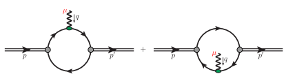
Figure 3: (Colour online) Feynman diagrams representing the electromagnetic current for a meson in our NJL model.

The electromagnetic current for a $\rho$-meson is parameterized by three form factors and takes the form:

$$j^{\mu,\alpha\beta}_{\rho}(p^{\prime},p) =\Big{[}g^{\alpha\beta}F_{1\rho}(Q^{2})-\frac{q^{\alpha}q^{\beta}}{2\,m_{\rho}^{2}}\,F_{2\rho}(Q^{2})\Big{]}\left(p^{\prime}+p\right)^{\mu}$$

$$-\left(q^{\alpha}g^{\mu\beta}-q^{\beta}g^{\mu\alpha}\right)F_{3\rho}(Q^{2}),$$ (14)

where the polarization of the incoming and outgoing $\rho$-meson is represented by the Lorentz indices $\alpha$ and $\beta$, respectively, and $\mu$ is the photon polarization. From these form factors one can define three Sachs form factors for the $\rho$, namely, the charge [$G_{C}(Q^{2})$]; the magnetic [$G_{M}(Q^{2})$] and quadrupole [$G_{Q}(Q^{2})$] form factors, which read

$$G_{C}(Q^{2}) =F_{1}(Q^{2})+\tfrac{2}{3}\eta\,G_{Q}(Q^{2}),$$ (15)

$$G_{M}(Q^{2}) =F_{3}(Q^{2}),$$ (16)

$$G_{Q}(Q^{2}) =F_{1}(Q^{2})+(1+\eta)\,F_{2}(Q^{2})-F_{3}(Q^{2}),$$ (17)

where $\eta=\tfrac{Q^{2}}{4\,m_{\rho}^{2}}$ and all form factors are dimensionless.

In our NJL model the $\rho$ electromagnetic current is depicted in Fig. 3 and expressed by

$$j^{\mu,\alpha\beta}_{\rho,ij}(p^{\prime},p)=i\int\frac{d^{4}k}{(2\pi)^{4}}$$

$$\hskip 4.2679pt\times\mathrm{Tr}\Big{[}\overline{\Gamma}_{\rho}^{\beta,j}\,S(p^{\prime}+k)\,\Lambda^{\mu}(p^{\prime},p)\,S(p+k)\,\Gamma_{\rho}^{\alpha,i}\,S(k)\Big{]}$$

$$+i\int\frac{d^{4}k}{(2\pi)^{4}}$$

$$\hskip 4.2679pt\times\mathrm{Tr}\Big{[}\Gamma_{\rho}^{\alpha,i}\,S(k-p)\,\Lambda^{\mu}(p^{\prime},p)\,S(k-p^{\prime})\,\overline{\Gamma}_{\rho}^{\beta,j}\,S(k)\Big{]},$$ (18)

where the Bethe-Salpeter vertices for the $\rho$ are given in Eq. (11), $\Lambda^{\mu}(p,p^{\prime})$ is the dressed quark-photon vertex and the trace is over Dirac, color and isospin indices. Following the calculations in Refs. Cloët et al. (2014); Ninomiya et al. (2015), we consider three versions of the quark-photon vertex, each of increasing sophistication; a pointlike quark-photon vertex; a vertex given by the solution of the inhomogeneous Bethe-Salpeter equation (illustrated in Fig. 4); and finally a quark-photon vertex which includes the pion cloud at the quark level (see Fig. 5).

The pointlike quark-photon is simply given by

$$\Lambda^{(\text{PL})\mu}(p,p^{\prime})=\left[\frac{1}{6}+\frac{\tau_{3}}{2}\right]\gamma^{\mu},$$ (19)

where $\tfrac{1}{6}+\tfrac{\tau_{3}}{2}$ is the quark charge operator. Projecting onto flavour sectors the vertex is separated into two components:

$$\Lambda^{(\text{PL})\mu}(p,p^{\prime})=\left[e_{u}\,\frac{1+\tau_{3}}{2}+e_{d}\,\frac{1-\tau_{3}}{2}\right]\gamma^{\mu},$$ (20)

where $e_{u}$ and $e_{d}$ are the charges of the $u$ and $d$ quarks, respectively.

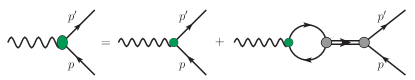
Figure 4: (Colour online) Inhomogeneous BSE whose solution gives the quark-photon vertex, represented as the large shaded oval. The small circle depicts the pointlike quark-photon driving term of Eq. (19), whereas the shaded circles with the double line represents the vector meson $t$-matrices.

In general the quark-photon vertex is dressed by $\bar{q}q$ interactions in the vector channel and in the NJL model this dressing is described by the corresponding inhomogeneous Bethe-Salpeter equation (see Fig. 4). From the NJL Lagrangian of Eq. (1) the contributions to this vertex come from the neutral vector mesons ($\rho^{0}$ and $\omega$). In the on-shell approximation for the external quarks, the solution of the inhomogeneous Bethe-Salpeter equation of Fig. 4 is

$$\Lambda^{(\text{bse})\mu}(p,p^{\prime})=\left[\frac{1}{6}\,F_{1\omega}(q^{2})+\frac{\tau_{3}}{2}\,F_{1\rho}(q^{2})\right]\gamma^{\mu},$$ (21)

where the dressed quark form factors are

$$F_{1\omega(\rho)}(q^{2})=\frac{1}{1+2\,G_{\omega(\rho)}\,\Pi_{VV}(q^{2})}.$$ (22)

Note, with the Lagrangian of Eq. (1) the inhomogeneous Bethe-Salpeter equation does not generate a Pauli form factor for the dressed quarks. Again projecting into flavour sectors gives

$$\Lambda^{(\text{bse})\mu}(p,p^{\prime})=\left[F^{\text{bse}}_{1U}(q^{2})\,\frac{1+\tau_{3}}{2}+F^{\text{bse}}_{1D}(q^{2})\,\frac{1-\tau_{3}}{2}\right]\gamma^{\mu},$$ (23)

where the dressed quark form factors are given by Cloët et al. (2014)

$$F^{\text{bse}}_{1U}(Q^{2}) =\frac{1}{6}F_{1\omega}(Q^{2})+\frac{1}{2}F_{1\rho}(Q^{2}),$$ (24)

$$F^{\text{bse}}_{1D}(Q^{2}) =\frac{1}{6}F_{1\omega}(Q^{2})-\frac{1}{2}F_{1\rho}(Q^{2}).$$ (25)

Finally we include pion loop corrections to the quark-photon vertex, as illustrated in Fig. 5, which give a vertex of the form

$$\Lambda^{\mu}(p,p^{\prime})=\Lambda^{\mu}_{U}(p,p^{\prime})\,\frac{1+\tau_{3}}{2}+\Lambda^{\mu}_{D}(p,p^{\prime})\,\frac{1-\tau_{3}}{2},$$ (26)

where the flavour sector vertices ($Q=U,\,D$) read

$$\Lambda^{\mu}_{Q}(p,p^{\prime})=\gamma^{\mu}\,F_{1Q}(q^{2})+\frac{i\sigma^{\mu\mu}q_{\nu}}{2\,M}\,F_{2Q}(Q^{2}).$$ (27)

Note that the pion cloud generates a Pauli form factor for the dressed quarks and that in obtaining Eq. (27) we have assumed the external quark lines are on-shell. The dressed quark form factors now read Cloët et al. (2014)

$$F_{1U} =Z\left[\tfrac{1}{6}F_{1\omega}+\tfrac{1}{2}F_{1\rho}\right]+\left[F_{1\omega}-F_{1\rho}\right]f_{1}^{q}+F_{1\rho}f_{1}^{\pi},$$ (28)

$$F_{1D} =Z\left[\tfrac{1}{6}F_{1\omega}-\tfrac{1}{2}F_{1\rho}\right]+\left[F_{1\omega}+F_{1\rho}\right]f_{1}^{q}-F_{1\rho}f_{1}^{\pi},$$ (29)

$$F_{2U} =\left[F_{1\omega}-F_{1\rho}\right]f_{2}^{q}+F_{1\rho}f_{2}^{\pi},$$ (30)

$$F_{2D} =\left[F_{1\omega}+F_{1\rho}\right]f_{2}^{q}-F_{1\rho}f_{2}^{\pi},$$ (31)

where for clarity we have dropped the explicit $Q^{2}$ dependence. The renormalization factor $Z$ is given by

$$Z=1+\left.\frac{\partial\Sigma(p)}{\partial\not{p}}\right|_{\not{p}=M},$$ (32)

where $\Sigma(p)$ is the self-energy from the pion cloud on a dressed quark:

$$\Sigma(p)=-\int\frac{d^{4}k}{(2\pi)^{4}}\,\gamma_{5}\,\tau_{i}\,S(p-k)\,\gamma_{5}\,\tau_{i}\,\tau_{\pi}(k).$$ (33)

Here the pion propagator is approximated by its pole form

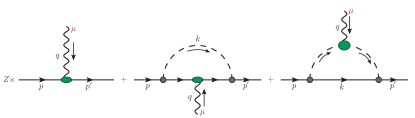
Figure 5: (Colour online) Pion cloud contribution to the quark-photon vertex. The quark-photon interaction in the first two diagrams, represented by the shaded ovals, is given by the solution of the inhomogeneous BSE. The last diagram also includes the pion form factor determined without the pion cloud on the associated dressed quarks.

$$\tau_{\pi}(k)\to\frac{i\,Z_{\pi}}{p^{2}-m_{\pi}^{2}+i\epsilon}.$$ (34)

The contributions of the pion cloud to the quark-photon vertex are contained in the functions $f_{i}^{q}(Q^{2})$ and $f_{i}^{\pi}(Q^{2})\leavevmode\nobreak\ (i=1,\,2)$ of Eqs. (28)-(31). These body form factors are associated with the second and third diagrams in Fig. 5, which are respectively expressed as

$$\Lambda_{Q}^{(q)\mu}(p^{\prime},p) =\gamma^{\mu}\,f_{1}^{q}(q^{2})+\frac{i\sigma^{\mu\nu}q_{\nu}}{2\,M}\,f_{2}^{q}(q^{2}),$$ (35)

$$\Lambda_{Q}^{(\pi)\mu}(p^{\prime},p) =\gamma^{\mu}\,f_{1}^{\pi}(q^{2})+\frac{i\sigma^{\mu\nu}q_{\nu}}{2\,M}\,f_{2}^{\pi}(q^{2}).$$ (36)

The analytic expressions read

$$\Lambda_{Q}^{(q)\mu}(p^{\prime},p) =\!\int\!\!\frac{d^{4}k}{(2\pi)^{4}}\,\gamma_{5}\,iS(p^{\prime}-k)\gamma^{\mu}\,iS(p-k)\gamma_{5}\,\tau_{\pi}(k),\allowdisplaybreaks$$ (37)

$$\Lambda_{Q}^{(\pi)\mu}(p^{\prime},p) =Z_{\pi}^{-1}\,(p^{\prime}+p)^{\mu}\,F_{\pi}^{(\text{PL})}(q^{2})$$

$$\times\int\frac{d^{4}k}{(2\pi)^{4}}\ \gamma_{5}\,\tau_{\pi}(p^{\prime}-k)\,\tau_{\pi}(p-k)\,\gamma_{5}\,iS(k),$$ (38)

where $F_{\pi}^{(\text{PL})}(q^{2})$ is the pion form factor determined with a pointlike quark-photon vertex.

For the full calculation of the $\rho$-meson form factors we use Eq. (18) and the quark-photon vertex given in Eq. (26). For the $\rho^{+}$ form factors this gives

$$F_{i\rho^{+}}(Q^{2}) =\left[F_{1U}(Q^{2})-F_{1D}(Q^{2})\right]f_{i}^{V}(Q^{2})$$

$$+\left[F_{2U}(Q^{2})-F_{2D}(Q^{2})\right]f_{i}^{T}(Q^{2}),$$ (39)

where $i=1,2,3$ indicates each of the three form factors of Eq. (14). The body form factors $f_{i}^{V}$ are associated with the vector part ($\gamma^{\mu}$) of the quark-photon vertex in Eq. (27), while $f_{i}^{T}$ are the body form factors associated with the tensor coupling ($\frac{i\sigma^{\mu\nu}q_{\nu}}{2\,M}$) in Eq. (27). To obtain the $\rho$-meson form factors that result only from the inhomogeneous BSE quark-photon vertex we then simply set $Z=1$ and the pion cloud contributions ($f_{1}^{q}(Q^{2})$, $f_{1}^{\pi}(Q^{2})$, etc) to zero. Finally, the $\rho$ form factors for a pointlike quark-photon vertex are then obtained by setting $F_{1\omega}=F_{1\rho}=1$. Note, all loop integrals are regularized using the proper-time scheme, with both an infrared and ultraviolet cutoff, except those of Eqs. (33), (37) and (III), where we take the infrared cutoff ($\Lambda_{IR}$) to zero as the pion should not be confined.

IV Results

$M$	$\Lambda_{IR}$	$\Lambda_{UV}$	$G_{\pi}$	$G_{\rho}$	$G_{\omega}$	$Z_{\pi}$	$Z_{\rho}$	$Z_{\omega}$
0.4	0.24	0.645	19.04	11.04	10.41	17.85	6.96	6.63

Table 1: Parameters of the model together with the effective couplings computed from Eqs. (12)-(13). The masses are in units of GeV, the Lagrangian couplings in units of GeV^-2 and the effective couplings are dimensionless.

The parameters of our model are the dressed quark mass $M$; the regularization cutoffs $\Lambda_{UV}$ and $\Lambda_{IR}$; and the Lagrangian couplings $G_{\pi}$, $G_{\rho}$ and $G_{\omega}$. For consistency with previous work we set $M=0.4$ GeV (in the physical limit: $m_{\pi}=140\,$MeV) and $\Lambda_{IR}=0.24\,$GeV Cloët et al. (2014); Ninomiya et al. (2015); Carrillo-Serrano et al. (2014). The ultraviolet cutoff $\Lambda_{UV}$ is fit to the physical value of the pion decay constant and the couplings $G_{\pi}$, $G_{\rho}$, and $G_{\omega}$ are fit to the physical masses of the $\pi$, $\rho$ and $\omega$ mesons using Eqs. (8)-(10). The values of these parameters, together with the quark-meson couplings of Eqs. (12)-(13), are given in Tab. 1.

Our purpose here is to compare results within this NJL model with other calculations, for example, constituent quark models García Gudiño and Toledo Sánchez (2014); Chung et al. (1988); Cardarelli et al. (1995); de Melo and Frederico (1997); Choi and Ji (1999); Melikhov and Simula (2002); Jaus (2003); Choi and Ji (2004); Biernat and Schweiger (2014), QCD sum rules Aliev et al. (2003); Samsonov (2003); Braguta and Onishchenko (2004); Aliev and Savci (2004), Dyson-Schwinger equations Hawes and Pichowsky (1999); Bhagwat and Maris (2008); Roberts et al. (2011); Pitschmann et al. (2013) and the recent lattice QCD studies Owen et al. (2015); Shultz et al. (2015). We first focus on static electromagnetic quantities for the $\rho^{+}$ meson and consider the magnetic moment ($\mu_{\rho}$), quadrupole moment ($\mathcal{Q}_{\rho}$) and rms charge radius ($\langle r_{C}^{2}\rangle$). These observables are defined by the Sachs form factors given in Eqs. (15)-(17), where the magnetic moment in nuclear magnetons ($\mu_{N}$) is given by $\mu_{\rho}=G_{M}(0)\tfrac{M_{N}}{m_{\rho}}$, with $M_{N}$ the physical nucleon mass and (for comparison with lattice data) $m_{\rho}$ is the $\rho$ mass evaluated at a particular pion mass; the quadrupole moment in units of $e/m^{2}_{\rho}$ is given by $\mathcal{Q}_{\rho}=G_{Q}(0)$; and finally the charge radius is defined by

$$\left<r_{C}^{2}\right>=\left.-6\,\frac{\partial\,G_{C}(Q^{2})}{\partial Q^{2}}\right|_{Q^{2}=0}.$$ (40)

In Tab. 2 we summarize results for the $\langle r_{C}^{2}\rangle$, $\mu_{\rho}$ and $\mathcal{Q}_{\rho}$ of the $\rho^{+}$ from various theoretical approaches, together with our calculations using the most sophisticated quark-photon vertex of Eq. (26) (BSE + pion cloud). In general including the dressing of the quark-photon vertex by the BSE and the pion cloud increases the magnitude of $\mu_{\rho}$ by 24%, $\mathcal{Q}_{\rho}$ by 22% and $\langle r_{C}^{2}\rangle$ by 16% Cloët et al. (2014).

Reference	$\langle r_{C}^{2}\rangle$(fm2)	$\mu_{\rho}$ ($\mu_{N}$)	$\mathcal{Q}_{\rho}$ (fm2)
This work	0.67	3.14	-0.070
Garcia Gudiño García Gudiño and Toledo Sánchez (2014)	–	2.6(6)	–
Cardarelli Cardarelli et al. (1995)	0.35	2.76	-0.024
De Melo de Melo and Frederico (1997)	0.37	2.61	-0.052
Melikhov Melikhov and Simula (2002)	0.33	2.87	-0.031
Jaus Jaus (2003)	–	2.23	-0.022
Choi Choi and Ji (2004)	–	2.34	-0.028
Biernat Biernat and Schweiger (2014)	–	2.68	-0.027
Samsonov Samsonov (2003)	–	2.4(4)	–
Aliev Aliev and Savci (2004)	–	2.8(6)	–
Hawes Hawes and Pichowsky (1999)	0.37	3.28	-0.055
Bhagwat Bhagwat and Maris (2008)	0.54	2.54	-0.026
Roberts Roberts et al. (2011)	0.31	2.14	-0.037
Pitschmann Pitschmann et al. (2013)	–	2.13	–
Owen Owen et al. (2015)	0.670(68)	2.613(97)	-0.0452(61)
Shultz Shultz et al. (2015)	0.30(6)	2.00(9)	-0.020(4)

Table 2: Comparison of the $\rho^{+}$ charge radius, magnetic moment and quadrupole moment for various theoretical approaches: phenomenological models García Gudiño and Toledo Sánchez (2014), constituent quark models Cardarelli et al. (1995); de Melo and Frederico (1997); Melikhov and Simula (2002); Jaus (2003); Choi and Ji (2004); Biernat and Schweiger (2014), QCD sum rules Samsonov (2003); Aliev and Savci (2004), Dyson Schwinger equations Hawes and Pichowsky (1999); Bhagwat and Maris (2008); Roberts et al. (2011); Pitschmann et al. (2013) and lattice QCD Owen et al. (2015); Shultz et al. (2015). The lightest pion mass used in the lattice calculation in Ref. Owen et al. (2015) is $m_{\pi}^{2}=0.026$ GeV², whereas for Ref. Shultz et al. (2015) it is $m_{\pi}^{2}=0.49$ GeV².

In comparing our results with lattice QCD we focus on the lattice simulation from Ref. Owen et al. (2015), as they extend to the lightest pion mass, namely, $m_{\pi}=161\,$MeV. Our computations as functions of $m_{\pi}^{2}$ are performed by keeping the regularization parameters ($\Lambda_{IR}$ and $\Lambda_{UV}$) and the couplings ($G_{\pi}$, $G_{\rho}$ and $G_{\omega}$) fixed, and varying the current quark mass that enters the gap equation. Results for the $\rho$ mass as a function of $m_{\pi}^{2}$ (or equivalently the current quark mass) are presented in Fig. 6, where we find remarkable agreement between our NJL calculation and the lattice results of Ref. Owen et al. (2015).

Figure 6: (Colour online) NJL model results for the $\rho$-meson mass versus $m_{\pi}^{2}$. Comparison is made with lattice results from Ref. Owen et al. (2015).

Figure 7: (Colour online) The squared charge radius $\langle r_{C}^{2}\rangle$ for the $\rho^{+}$ meson computed using the three levels of sophistication for the quark-photon vertex: pointlike (PL), using the inhomogeneous BSE (BSE) and including the pion cloud (BSE + pion cloud). Comparison is made with lattice results from Ref. Owen et al. (2015).

At the physical pion mass our values for $\langle r_{C}^{2}\rangle$ (see Tab. 2) differ significantly from the constituent quark models, one of the Dyson-Schwinger calculations and the result quoted in the lattice QCD computation of Ref. Shultz et al. (2015). Better agreement is seen with the Dyson-Schwinger equation calculation of Ref. Bhagwat and Maris (2008). Our result for $\langle r_{C}^{2}\rangle$ is however very similar to the lattice QCD value obtained in Ref. Owen et al. (2015) for a pion mass of around $161$ MeV. We see that in Fig. 7 their $\langle r_{C}^{2}\rangle$ lies around $0.67$ fm², possibly reaching $0.7$ fm² in the physical limit. On the other hand the lattice QCD simulation of Ref. Shultz et al. (2015) uses a very large pion mass of $700$ MeV, which explains its lower value for $\langle r_{C}^{2}\rangle$, evident from the $m_{\pi}^{2}$ dependence of the lattice points in Fig. 7. The dependence of $\langle r_{C}^{2}\rangle$ on $m_{\pi}^{2}$ in our NJL calculation, once the inhomogeneous BSE and pion cloud contributions have been included, shows remarkable agreement with the lattice results of Ref. Owen et al. (2015). One sees that the pion cloud contributions have become negligible for $m_{\pi}^{2}\gtrsim 0.4\,$GeV².

Figure 8: (Colour online) The $\rho^{+}$ magnetic moment ($\mu_{\rho}$) versus $m_{\pi}^{2}$. The curves have the same conventions as Fig. 7.

Figure 9: (Colour online) The $\rho^{+}$ quadrupole moment ($\mathcal{Q}_{\rho}$) versus $m_{\pi}^{2}$. The curves have the same conventions as Fig. 7.

For the $\rho^{+}$ magnetic moment ($\mu_{\rho}$) the values obtained by the constituent quark models are consistently smaller than our result of $\mu_{\rho}=3.14\,\mu_{N}$, the closest being $\mu_{\rho}=2.87\,\mu_{N}$ from Ref. Melikhov and Simula (2002). The earlier Dyson-Schwinger equation study in Ref. Hawes and Pichowsky (1999) shows good agreement with our work. For the lattice simulation of Ref. Owen et al. (2015) the discrepancy with our result is sizeable near the physical limit. However, the evolution of our result with $m_{\pi}^{2}$ shown in Fig. 9 is in good agreement with the lattice QCD calculations except at their lightest pion mass. Again, as in the case of $\langle r_{C}^{2}\rangle$, the effect of the large $m_{\pi}$ in Ref. Shultz et al. (2015) is to produce a small value of $\mu_{\rho}$, as evident from Fig. 9.

Figure 10: (Colour online) The $\rho^{+}$ Sachs form factors as a functions of $m_{\pi}^{2}$ at $Q^{2}=0.16$ GeV². The curves have the same conventions as Fig. 7.

Finally we find a large quadrupole moment comparable to the Dyson-Schwinger equation results of Roberts et al. Roberts et al. (2011) and Hawes et al. Hawes and Pichowsky (1999). The lattice QCD result of Ref. Owen et al. (2015) is approximately $\sim\!30\%$ smaller than our result near the physics point, as illustrated in Fig. 9. However, as a hypothesis for the difference we suggest that it may be worthwhile to investigate the effect of the lack of spherical symmetry on the lattice simulation, considering that the quadrupole moment reflects the shape of the $\rho$.

Figure 11: (Colour online) The $\rho^{+}$ Sachs form factors for $m_{\pi}^{2}=0.49$ GeV². Comparison is made with lattice results from Ref. Shultz et al. (2015) and the curves have the same conventions as Fig. 7.

Comparison with the lattice simulation of Ref. Owen et al. (2015) for the evolution of the $\rho^{+}$ Sachs form factors with $m_{\pi}^{2}$, at a fixed $Q^{2}=0.16\,$GeV², is made in Figs. 10. The charge form factor, $G_{C}$, is in good agreement with the lattice QCD points, when both the inhomogeneous BSE and pion cloud dressing are included. On the other hand, for the magnetic form factor $G_{M}$, the BSE results alone have better agreement with lattice and the pion cloud causes an overestimate. The deviations are still small however, considering the simplicity of the calculation. The deviation from the lattice simulation data for $G_{Q}$ is possibly explained by the same reason behind the disagreement with $\mathcal{Q}_{\rho}$, that is, the lack of spherical symmetry in the lattice simulation.

A final comparison is made in Fig. 11 for the Sachs form factors as a function of $Q^{2}$ for a pion mass of $m_{\pi}^{2}=0.49$ GeV², where the lattice results are from Ref. Shultz et al. (2015). We find that our model qualitatively describes the $\rho^{+}$ form factors obtained from the lattice computation. Once again the addition of the pion cloud causes an overestimate of $G_{M}(Q^{2})$ and the magnitude of $G_{Q}(Q^{2})$ also appears too large.

V CONCLUSIONS

We computed the electromagnetic form factors of the $\rho^{+}$ meson using an NJL model that simulates aspects of quark confinement. The quark-photon vertex is studied in three levels of sophistication: pointlike dressed quark, via the inhomogeneous BSE and also including corrections from a pion cloud. The results are qualitatively in good agreement with the recent lattice QCD computations.

The main level of disagreement comes from the quadrupole moment and the corresponding form factor. We suggest that lattice QCD studies of this type should look at the possible effects of the lack of spherical symmetry of a cubic lattice in the quadrupole moments and form factors. It would certainly be helpful to have further lattice studies over a range of pion masses and momentum transfers. Experimental measurements would also be extremely valuable.

Therefore, the present work on the $\rho$-meson structure and the progress in the computation of the electromagnetic form factors of the $\pi$ and $K$, including the pion cloud, reported in Ref. Ninomiya et al. (2015), support the importance of the model as a tool to describe hadronic structure. In addition, the NJL model is a quantum field theory where calculations are relatively straightforward and it gives good results when compared to more sophisticated methods that require much more resources, such as lattice QCD. These advantages are useful in order to perform larger calculations in problems such as the description of hadrons in the nuclear medium, as required, for example, to explore the properties of neutron stars. In such cases the NJL model serves as a very useful tool to guide possible future computations of lattice QCD and other more sophisticated approaches.

- (1) A. W. Thomas and W. Weise, The Structure of the Nucleon (Wiley-VCH, Berlin, 2001).
- Olive et al. (2014) K. Olive et al. (Particle Data Group), Chin. Phys. C38, 090001 (2014).
- Aubert et al. (2008) B. Aubert et al. (BaBar), Phys. Rev. D78, 071103 (2008) [arXiv:0806.3893 [hep-ex]].
- Dbeyssi et al. (2012) A. Dbeyssi, E. Tomasi-Gustafsson, G. Gakh and C. Adamuscin, Phys.Rev. C85, 048201 (2012) [arXiv:1112.6248 [hep-ph]].
- Adamuscin et al. (2007) C. Adamuscin, G. Gakh and E. Tomasi-Gustafsson, Phys. Rev. C75, 065202 (2007) [arXiv:0706.1125 [hep-ph]].
- García Gudiño and Toledo Sánchez (2014) D. García Gudiño and G. Toledo Sánchez, Int. J. Mod. Phys. Conf. Ser. 35, 1460463 (2014) [arXiv:1305.6345 [hep-ph]].
- Chung et al. (1988) P. Chung, W. Polyzou, F. Coester and B. Keister, Phys. Rev. C37, 2000 (1988).
- Cardarelli et al. (1995) F. Cardarelli, I. Grach, I. Narodetsky, G. Salme and S. Simula, Phys. Lett. B349, 393 (1995) [arXiv:hep-ph/9502360 [hep-ph]].
- de Melo and Frederico (1997) J. de Melo and T. Frederico, Phys. Rev. C55, 2043 (1997) [arXiv:nucl-th/9706032 [nucl-th]].
- Choi and Ji (1999) H.-M. Choi and C.-R. Ji, Phys. Rev. D59, 074015 (1999) [arXiv:hep-ph/9711450 [hep-ph]].
- Melikhov and Simula (2002) D. Melikhov and S. Simula, Phys. Rev. D65, 094043 (2002) [arXiv:hep-ph/0112044 [hep-ph]].
- Jaus (2003) W. Jaus, Phys. Rev. D67, 094010 (2003) [arXiv:hep-ph/0212098 [hep-ph]].
- Choi and Ji (2004) H.-M. Choi and C.-R. Ji, Phys. Rev. D70, 053015 (2004) [arXiv:hep-ph/0402114 [hep-ph]].
- Biernat and Schweiger (2014) E. P. Biernat and W. Schweiger, Phys. Rev. C89, 055205 (2014) [arXiv:1404.2440 [hep-ph]].
- Aliev et al. (2003) T. Aliev, I. Kanik and M. Savci, Phys. Rev. D68, 056002 (2003) [arXiv:hep-ph/0303068 [hep-ph]].
- Samsonov (2003) A. Samsonov, JHEP 0312, 061 (2003) [arXiv:hep-ph/0308065 [hep-ph]].
- Braguta and Onishchenko (2004) V. Braguta and A. Onishchenko, Phys.Rev. D70, 033001 (2004) [arXiv:hep-ph/0403258 [hep-ph]].
- Aliev and Savci (2004) T. Aliev and M. Savci, Phys. Rev. D70, 094007 (2004) [arXiv:hep-ph/0405235 [hep-ph]].
- Hawes and Pichowsky (1999) F. Hawes and M. Pichowsky, Phys.Rev. C59, 1743 (1999) [arXiv:nucl-th/9806025 [nucl-th]].
- Bhagwat and Maris (2008) M. Bhagwat and P. Maris, Phys. Rev. C77, 025203 (2008) [arXiv:nucl-th/0612069 [nucl-th]].
- Roberts et al. (2011) H. Roberts, A. Bashir, L. Gutierrez-Guerrero, C. Roberts and D. Wilson, Phys. Rev. C83, 065206 (2011) [arXiv:1102.4376 [nucl-th]].
- Pitschmann et al. (2013) M. Pitschmann, C.-Y. Seng, M. J. Ramsey-Musolf, C. D. Roberts, S. M. Schmidt et al., Phys.Rev. C87, 015205 (2013) [arXiv:1209.4352 [nucl-th]].
- Andersen and Wilcox (1997) W. Andersen and W. Wilcox, Annals Phys. 255, 34 (1997) [arXiv:hep-lat/9502015 [hep-lat]].
- Hedditch et al. (2007) J. Hedditch, W. Kamleh, B. Lasscock, D. Leinweber, A. Williams et al., Phys. Rev. D75, 094504 (2007) [arXiv:hep-lat/0703014 [HEP-LAT]].
- Owen et al. (2015) B. Owen, W. Kamleh, D. Leinweber, B. Menadue and S. Mahbub, Phys. Rev. D91, 074503 (2015) [arXiv:1501.02561 [hep-lat]].
- Shultz et al. (2015) C. J. Shultz, J. J. Dudek and R. G. Edwards, arXiv:1501.07457 [hep-lat].
- Cloët et al. (2014) I. C. Cloët, W. Bentz and A. W. Thomas, Phys. Rev. C90, 045202 (2014) [arXiv:1405.5542 [nucl-th]].
- Nambu and Jona-Lasinio (1961a) Y. Nambu and G. Jona-Lasinio, Phys. Rev. 122, 345 (1961a).
- Nambu and Jona-Lasinio (1961b) Y. Nambu and G. Jona-Lasinio, Phys. Rev. 124, 246 (1961b).
- Ninomiya et al. (2015) Y. Ninomiya, W. Bentz and I. C. Cloët, Phys. Rev. C91, 025202 (2015) [arXiv:1406.7212 [nucl-th]].
- Klevansky (1992) S. Klevansky, Rev. Mod. Phys. 64, 649 (1992).
- Ebert et al. (1996) D. Ebert, T. Feldmann and H. Reinhardt, Phys. Lett. B 388, 154 (1996) [arXiv:9608223 [hep-ph]].
- Hellstern et al. (1997) G. Hellstern, R. Alkofer and H. Reinhardt, Nucl. Phys. A 625, 697 (1997) [arXiv:9706551 [hep-ph]].
- Bentz and Thomas (2001) W. Bentz and A. W. Thomas, Nucl. Phys. A 696, 138 (2001) [arXiv:0105022 [nucl-th]].
- Hatsuda and Kunihiro (1994) T. Hatsuda and T. Kunihiro, Phys. Rept. 247, 221 (1994) [arXiv:9401310 [hep-ph]].
- Vogl and Weise (1991) U. Vogl and W. Weise, Prog. Part. Nucl. Phys. 27, 195 (1991).
- Cloët et al. (2005a) I. C. Cloët, W. Bentz and A. W. Thomas, Phys. Lett. B621, 246 (2005a) [arXiv:0504229 [hep-ph]].
- Cloët et al. (2005b) I. C. Cloët, W. Bentz and A. W. Thomas, Phys. Rev. Lett. 95, 052302 (2005b) [arXiv:0504019 [nucl-th]].
- Cloët et al. (2008) I. C. Cloët, W. Bentz and A. W. Thomas, Phys. Lett. B659, 214 (2008) [arXiv:0708.3246 [hep-ph]].
- Bentz et al. (2008) W. Bentz, I. C. Cloët, T. Ito, A. W. Thomas and K. Yazaki, Prog. Part. Nucl. Phys. 61, 238 (2008) [arXiv:0711.0392 [nucl-th]].
- Matevosyan et al. (2012) H. H. Matevosyan, W. Bentz, I. C. Cloët and A. W. Thomas, Phys. Rev. D85, 014021 (2012) [arXiv:1111.1740 [hep-ph]].
- Carrillo-Serrano et al. (2014) M. E. Carrillo-Serrano, I. C. Cloët and A. W. Thomas, Phys. Rev. C90, 064316 (2014) [arXiv:1409.1653 [hep-th]].
- Liu et al. (2015) Z.-W. Liu, M. E. Carrillo-Serrano and A. W. Thomas, Phys. Rev. D91, 014028 (2015) [arXiv:1409.2639 [hep-ph]].