Stochastic focusing coupled with negative feedback enables robust regulation in biochemical reaction networks

Abstract

Nature presents multiple intriguing examples of processes which proceed at high precision and regularity. This remarkable stability is frequently counter to modelers’ experience with the inherent stochasticity of chemical reactions in the regime of low copy numbers. Moreover, the effects of noise and nonlinearities can lead to “counter-intuitive” behavior, as demonstrated for a basic enzymatic reaction scheme that can display stochastic focusing (SF). Under the assumption of rapid signal fluctuations, SF has been shown to convert a graded response into a threshold mechanism, thus attenuating the detrimental effects of signal noise. However, when the rapid fluctuation assumption is violated, this gain in sensitivity is generally obtained at the cost of very large product variance, and this unpredictable behavior may be one possible explanation of why, more than a decade after its introduction, SF has still not been observed in real biochemical systems.

In this work we explore the noise properties of a simple enzymatic reaction mechanism with a small and fluctuating number of active enzymes that behaves as a high-gain, noisy amplifier due to SF caused by slow enzyme fluctuations. We then show that the inclusion of a plausible negative feedback mechanism turns the system from a noisy signal detector to a strong homeostatic mechanism by exchanging high gain with strong attenuation in output noise and robustness to parameter variations. Moreover, we observe that the discrepancy between deterministic and stochastic descriptions of stochastically focused systems in the evolution of the means almost completely disappears, despite very low molecule counts and the additional nonlinearity due to feedback.

The reaction mechanism considered here can provide a possible resolution to the apparent conflict between intrinsic noise and high precision in critical intracellular processes.

1 Introduction

Random fluctuations due to low-copy number phenomena inside the microscopic cellular volumes have been an object of intense study in recent years. It is now widely recognized that deterministic modeling of chemical kinetics is in many cases inadequate for capturing even the mean behavior of stochastic chemical reaction networks, and several studies have explored the discrepancy between deterministic and stochastic system descriptions [1, 23, 33, 26].

Despite the all-pervasive stochasticity, cellular processes and responses proceed with surprising precision and regularity, thanks to efficient noise suppression mechanisms also present within cells. The structure and function of these mechanisms has been a topic of great interest [7, 2, 32, 31, 15, 22, 3, 26], and in many cases still remains unknown.

Moreover, recent theoretical works on enzymatic reaction schemes with a single or a few enzyme molecules [18, 11, 13, 29] have repeatedly shown that low-copy enzymatic reactions demonstrate a stochastic behavior that can lead to markedly different responses in comparison to the predictions of deterministic enzyme kinetic models.

In this work we investigate the properties of a possible noise suppression mechanism for an enzymatic reaction with a small and fluctuating number of active enzymes. Under certain conditions, presented in [23], this system displays an increased sensitivity to enzyme fluctuations, a phenomenon that has been termed stochastic focusing.

Stochastic focusing has been presented as a possible mechanism for sensitivity amplification: compared to a deterministic model of a biochemical network, the mean output of the stochastic version of the system can display increased sensitivity to changes in the input, when the input species has sufficiently low abundance. Consequently, it has been postulated that stochastic focusing can act as a signal detection mechanism, that converts a graded input into a “digital” output.

The basic premise of [23] has been that fluctuations in the “input” species are sufficiently rapid, so that any rates that depend on the signaling species show minimal time-correlations. We show that if this condition fails, i.e. when the fluctuations in the input signal are slow compared to the average lifetime of a substrate molecule, stochastic focusing can result in a dramatic increase in substrate fluctuations, a fact also acknowledged in the original publication. Increased sensitivity to input changes does not only come at the cost of extremely high output noise levels; as we will demonstrate here, systems operating in this regime are also extremely sensitive to variations in reaction rates, which in fact precludes robust signal detection by stochastic focusing.

For the first time since its introduction we could study the steady-state behavior of this system analytically, by formulating and solving the equations for the conditional means and (co)variances [3]. Motivated by our observations on the open-loop, stochastically focused system, we investigated the system behavior in the presence of a plausible feedback mechanism. We treated the enzyme as a noisy “controller” molecule whose purpose is to regulate the outflux of a reaction product by – directly or indirectly – “sensing” the fluctuations in its substrate. For the sake of simplicity and clarity, we focused on very simple and highly abstracted mechanisms, but we should remark that several possible biochemical implementations of our feedback mechanism can be considered.

Our premise was that the great open-loop sensitivity of a stochastically focused system with relatively slow input fluctuations creates a system with very high open-loop gain, which in turn can be exploited to generate a very robust closed-loop system once the output is connected to the input. Our simulation results confirmed this intuition, revealing a dramatic decrease in noise levels and a significant increase in robustness in the steady-state mean behavior of the closed-loop system. Such a system no longer functions as a signal detector, but rather behaves as a strong homeostatic mechanism. Moreover, we observed that the steady-state behavior of the means in a stochastically focused system with feedback can be captured quite accurately by the corresponding deterministic system of reaction rate equations, despite the fact that the stochastic system still operates at very low copy numbers.

Noise attenuation through feedback and the fundamental limits of any feedback system implemented with noisy “sensors” and “controllers” have been studied theoretically in the recent years, and some fairly general performance bounds have been derived in [19]. We should note that, despite its generality, the modeling framework assumed in [19] does not apply in our case, since our system contains a controlled degradation reaction, whereas [19] considers only control of production. More specifically, [19] examines the case where a given species regulates its own production through an arbitrary stochastic signaling network. In this setting, it is shown that, no matter the form or complexity of the intermediate signaling, the loss of information induced by stochasticity places severe fundamental limits on the levels of noise suppression that such feedback loops can achieve. On the other hand, it is still unclear what type of noise suppression limitations are present for systems such as the one studied here, and a complete analytical treatment of the problem of regulated substrate degradation seems very difficult at the moment.

A first attempt to analyze the noise properties of regulated degradation was presented in [7], which examined such a scheme using the Linear Noise Approximation (LNA) [9]. As the authors of that work pointed out, however, the LNA is incapable of correctly capturing the system behavior (i.e. means and variances) beyond the small-noise regime, due to the nonlinear system behavior. We verified this inadequacy, not only for LNA, but for other approximation schemes as well, such as the Langevin equations [21] and various moment closure approaches [30]. Perhaps this is the reason why, contrary to regulated production, the theoretical noise properties of regulated substrate degradation have received relatively little attention.

With the rapid advancement of single-molecule enzymatic assays [27, 20], we expect that the study of noise properties of various low-copy enzymatic reactions, including the proposed feedback mechanism described here, will soon be amenable to experimental verification. It also remains to be seen whether the proposed feedback mechanism is actually employed by cells to achieve noise attenuation in enzymatic reactions. At any rate, the noise attenuation scheme presented here could be tried and tested in synthetic circuits through enzyme engineering [24, 4].

2 Results

2.1 A slowly fluctuating enzymatic reaction scheme that exhibits stochastic focusing

In this section we formulate and analyze a simple biochemical reaction network capable of exhibiting the dynamic phenomenon of stochastic focusing. It is shown that in the stochastic focusing regime, the system acts as a noisy amplifier with an inherent strong sensitivity to perturbations. It follows that without modifications, the network cannot be used under conditions requiring precision and regularity.

2.1.1 Modeling

We consider the simple branched reaction scheme studied in [23] and shown schematically in Fig. 1(a). In this scheme, substrate molecules $C$ enter the system at a constant influx, and can either be converted into a product $P$ or degraded under the action of a low-copy enzyme (or, equivalently, converted into a product that leaves the system). While the number of enzymes in the system is assumed constant, enzyme molecules can spontaneously fluctuate between an active ($E^{*}$) and an inactive ($E$) form. The generality of this model and its sensitivity to variations in the active enzyme levels is further discussed in the Supplement (sections 1 and 2).

Recent single-enzyme turnover experiments have shown that single enzyme molecules typically fluctuate between conformations with different catalytic activities, a phenomenon called dynamic disorder [18, 11, 13, 29]. In the simple model considered here, the enzyme randomly switches between two activity states. The stationary distribution of $E^{*}$ in this case is known to be binomial [35]; that is, $E^{*}\sim\mbox{B}(N,p)$, where $N=E+E^{*}$ is the total number of enzymes in the system and $p=\alpha_{E}/(\alpha_{E}+\mu_{E})$, such that the mean $\langle E^{*}\rangle=Np$.

The basic (empirically derived) conditions for stochastic focusing [23] are that the magnitude of active enzyme fluctuations is significant compared to the mean number of active enzymes, while the total number of enzymes is low. Moreover, it is assumed that the level of $E^{*}$ fluctuates rapidly compared to the average lifetime of $C$ and $P$ molecules. Without this assumption, the noise in $E^{*}$ can be greatly amplified by $C$ and transmitted to $P$.

The first assumption (large enzyme fluctuations and low abundance) is maintained in our setup. However, we shall dispense with the second assumption. We further postulate that $C$ (possibly a product of upstream enzymatic reactions) enters the system at a high input flux (large $\alpha_{C}$) and that there exists a strong coupling between $C$ and $E^{*}$, in the sense that a few active enzymes can strongly affect the degradation of $C$.

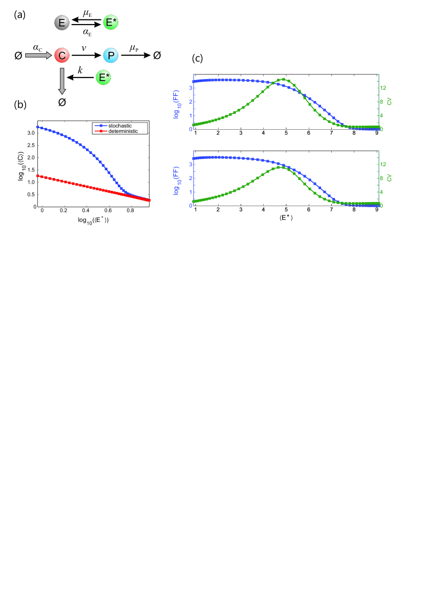
Figure 1: (a) The reaction scheme studied in this work. Thick arrows represent high-flux reactions. (b) Blue line: Steady-state mean of $C$ (denoted by $\langle C\rangle$ throughout) as a function of the average number of active enzyme molecules ($N\alpha_{E}/(\alpha_{E}+\mu_{E}))$ for $N=10,~{}\mu_{E}=0.1,~{}\alpha_{C}=5010,~{}k=300,~{}\nu=1,~{}\mu_{P}=1$. Since $\nu=\mu_{P}$, the average of $P$ displays the same behavior as the substrate. Red line: Steady-state of the ODE model for the same parameter values. The large difference (notice the logarithmic scale) between the blue and red lines is a consequence of stochastic focusing [23]. (c) Upper: Substrate ($C$) noise statistics as a function of the average number of active enzymes. Blue: Steady-state Fano factor (variance/mean; notice the logarithmic scale). Green: Steady-state coefficient of variation (standard deviation/mean). Lower: Product ($P$) noise statistics as a function of the average number of active enzymes. Color coding same as in upper panel. Both plots were obtained for $N=10,~{}\mu_{E}=0.1,~{}\alpha_{C}=5010,~{}k=300,~{}\nu=1,~{}\mu_{P}=1$. All calculations were performed analytically, using the conditional moment equations and the known stationary distribution of $E^{*}$.

More concretely, the previously stated assumptions imply that the reaction rates must satisfy the following conditions:

1. $\alpha_{C}\gg 1$ (high influx of $C$)

2. $k\gg\alpha_{E}+\mu_{E}$ (enzyme fluctuations are slow compared to the average lifetime of a substrate molecule)

3. $k\gg 1$ (strong coupling between enzyme and substrate)

4. $Np=N\displaystyle\frac{\alpha_{E}}{\alpha_{E}+\mu_{E}}$ is small (e.g. below 10).

These conditions are motivated via a short theoretical and numerical analysis in the Supplement (section 1). When they hold, we expect the amount of $C$ to fluctuate wildly as $E^{*}$ varies over time and these fluctuations to propagate to $P$. In the rest, we will refer to this motif as the (open-loop) slowly fluctuating enzyme (SFE) system.

The computational analysis of this and similar systems has thus far been hindered by the presence of the bimolecular reaction, which leads to statistical moment equations that are not closed [30], while the presence of stochastic focusing presents further difficulties for any moment closure method. In this work, we circumvent these difficulties by formulating and solving the conditional moment equations [3] for the means and (co)variances of $C$ and $P$ conditioned on the enzyme state (whose steady-state distribution is known). This enables for the first time the analytical study of the steady-state behavior of this system (more details can be found in the Supplement, section 3). Chiefly, the equations for the first two conditional moments of the SFE system are in fact closed, i.e. they do not depend on moments of order higher than 2, and thus do not require a moment closure approximation despite the fact that the unconditional moment equations themselves are open. We next use these analytic equations to shed new light on the properties of the network under consideration.

2.1.2 The SFE system functions as a noisy amplifier

According to the method of conditional moments (MCM) [3], the chemical species of a given system are divided into two classes. Species of the first class, collectively denoted by $Y$, are treated fully stochastically, while species of the second class, denoted by $Z$, are described through their conditional moments given $Y$. More analytically, the MCM considers a chemical master equation (CME) [36] for the marginal distribution of $Y$, $p(Y,t)=\sum_{Z\geq 0}p(Y,Z,t)$, and a system of conditional means ($\mu_{Z}(Y,t):=\mathbb{E}_{p(Z|Y,t)}[Z|Y,t]$) and higher-ordered centered moments (e.g. conditional variances $C_{Z}(Y,t):=\mathbb{E}_{p(Z|Y,t)}[(Z-\mu_{Z}(Y,t))^{2}|Y,t]$) for the $Z$ species. In the case of the SFE network, by taking $Y=E^{*}$ and $Z=(C,P)$, we see that $Y$ is independent of $Z$ and its evolution is described by a CME whose stationary solution is known. Moreover, the system of conditional means and (co)variances of $Z$ given $Y$ turns out to be closed.

We thus begin by examining the behavior of the system as the enzyme activation rate is varied while keeping other parameters unchanged. Assuming a fixed $\mu_{E}$, $\alpha_{E}$ is directly related to $\langle E^{*}\rangle$, the average number of active enzymes. Thus, any changes in $\langle E^{*}\rangle$ are assumed to be driven by $\alpha_{E}$, which means that the two can be used interchangeably. We present the performance of the open-loop system with respect to $\langle E^{*}\rangle$ wherever possible, as we find this more intuitive.

The results in Fig. 1(b) show that the stationary means of $C$ and $P$ (denoted by angle brackets throughout the paper) depend very sensitively on $\langle E^{*}\rangle$, as one would expect from a stochastically focused system. Moreover, owing to the relatively slow switching frequency of enzyme states, the stationary distributions of substrate and product are greatly over-dispersed, as shown in Fig. 1(c).

Apart from the enzyme activation rate, the catalytic degradation rate ($k$) is also expected to affect noise in the system, as it controls both the timescale and magnitude of substrate fluctuations: as $k$ increases, the rate of substrate consumption grows as well. On the other hand, the impact of a change in the number of active enzymes is also magnified. We can study the interplay of $\alpha_{E}$ and $k$ by varying both simultaneously, as shown in Fig. 2(a). Although $\alpha_{E}$ has a much more pronounced effect on substrate and product means and variances, the interplay of $k$ and $\alpha_{E}$ is what determines the overall noise strength in the system, as the third row of plots shows.

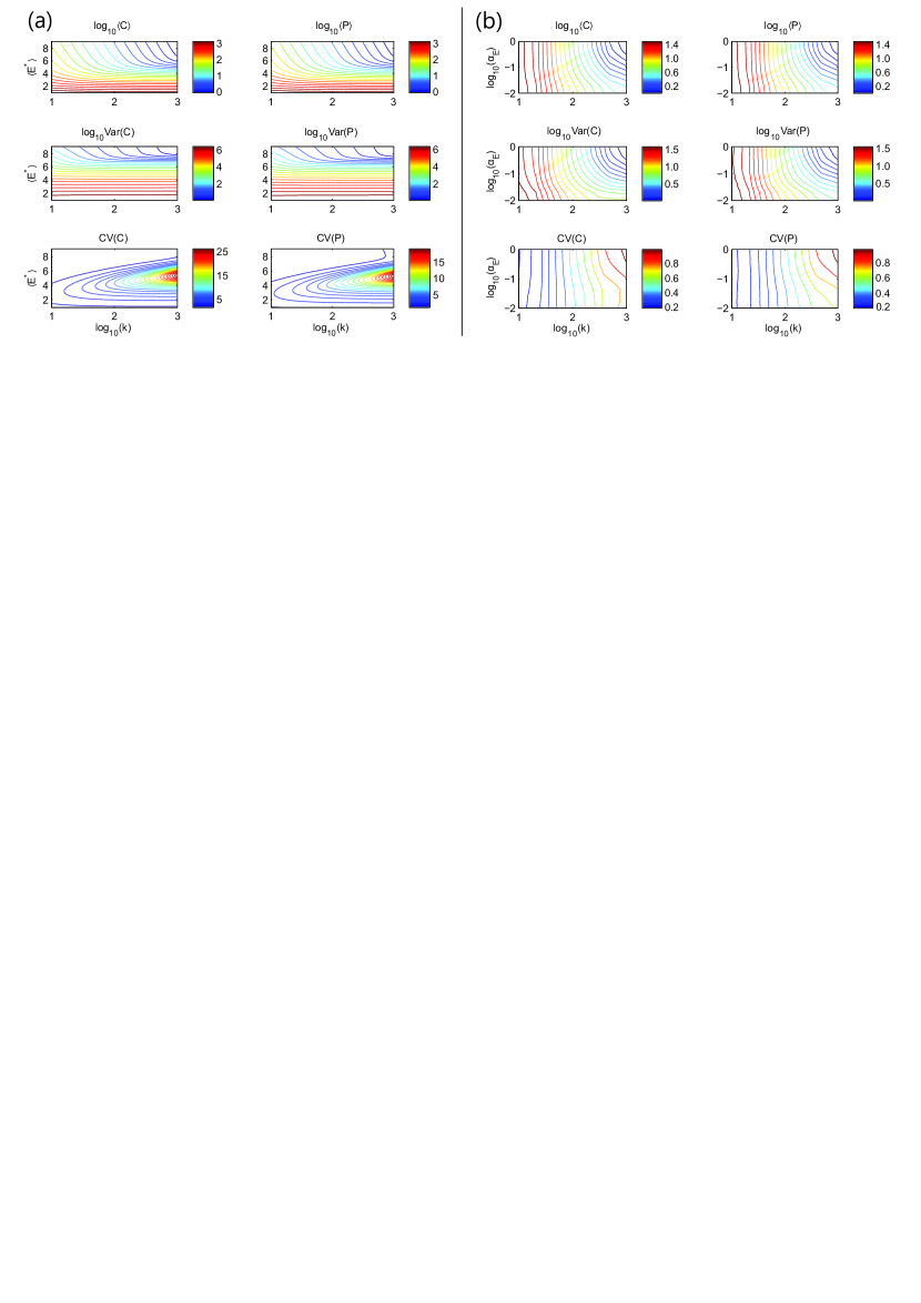
Figure 2: (a) Steady-state means, variances and CVs of substrate and product as a function of the average active enzymes ($\alpha_{E}N/(\alpha_{E}+\mu_{E})$) and $k$ for $N=10,~{}\mu_{E}=0.1,~{}\alpha_{C}=5010,~{}\nu=1,~{}\mu_{P}=1$ (notice the logarithmic scales). (b) Closed-loop SFE system with substrate feedback: steady-state means, variances and CVs of substrate and product as a function of $\alpha_{E}$ (which determines the average number of active enzymes) and $k$ for $K=3,~{}C_{0}=5,~{}N=10,~{}\mu_{E}=0.1,~{}\alpha_{C}=5010,~{}\nu=1,~{}\mu_{P}=1$. Logarithmic scales are preserved to make comparisons with Fig. 2 easier, although the range of variation is much smaller in this case.

From the above analysis, we deduce that the open-loop motif amplifies both small changes in the average number of active enzymes (Fig. 1(b)), as well as temporal fluctuations in the active enzyme levels (Fig. 1(c)): for intermediate values of $\alpha_{E}$, the CV and FF of $C$ and $P$ are much greater than zero. This implies that the instantaneous flux of substrate through the two alternative pathways experiences very large fluctuations, which would propagate to any reactions downstream of $C$.

2.1.3 The SFE system is very sensitive to parameter perturbations

The increased sensitivity of the SFE network to fluctuations in the active enzyme would suggest sensitivity with respect to variations in reaction rates. To verify this, we generated 10000 uniformly distributed joint random perturbations of all system parameters that reach up to 50% of their nominal values. That is, every parameter was perturbed according to the following scheme:

$$p_{pert}=p_{nom}+(n-0.5)p_{nom},~{}n\sim\mathcal{U}([0,1]).$$ (1)

For each perturbed parameter set, the steady-state conditional moment equations were solved to obtain the means, variances and noise measures for both the substrate and product. The results are summarized in Fig. 3 (dashed lines), where the large parametric sensitivity of the system can be clearly seen. Global sensitivity analysis of the mean, variance and CV histograms [25] reveals that the total number of enzymes ($N$) has the largest effect on all these quantities, with the enzyme activation/deactivation rates ($\alpha_{E},~{}\mu_{E}$) coming at second and third place. Although one could argue that $\alpha_{E}$ and $\mu_{E}$ are biochemical rates that are uniquely determined by molecular features of the enzyme, the total number of enzyme molecules would certainly be variable across a cellular population.

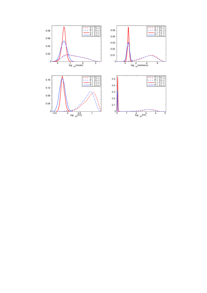
Figure 3: Dashed lines: Histograms of steady-state means, variances, CVs and Fano Factors of substrate and product, obtained from 10000 randomly sampled parameters, following (1). Nominal values of perturbed parameters: $N=10,~{}\alpha_{E}=0.08,~{}\mu_{E}=0.1,~{}\alpha_{C}=5010,~{}k=300,~{}\nu=1,~{}\mu_{P}=1$. The black line on the top left plot denotes the (common) mean of substrate and product for the nominal parameters. On the top right plot, black lines mark the nominal variance for substrate (solid) and product (dashed). Continuous lines: Closed-loop SFE system ($K=3,~{}C_{0}=5$) with substrate feedback: Histograms of steady-state means, variances, CVs and FFs of substrate and product

, obtained from the same 10000 randomly sampled parameters used for the dashed line histograms. The great reduction in sensitivity of the closed-loop SFE system in comparison to the open-loop can be easily observed.

Taken together, the results of this section and the previous one suggest that the operation of the SFE reaction scheme in Fig. 1(a) as a signal detection mechanism (the original point made in [23]) is severely compromised when the system operates in the regime defined by our set of assumptions: besides amplifying enzyme fluctuations, the system responds very sensitively to parametric perturbations. These features render the enzyme a highly non-robust controller of the substrate and product outfluxes, which can fluctuate dramatically in time. In addition, reaction rates have to be very finely tuned to achieve a certain output behavior, for example a given mean and variance, or a given average substrate outflux.

2.2 Closing the loop: The SFE network with negative feedback

It is a well-known fact in control theory that negative feedback results in a reduction of the closed-loop system gain [6, 17]. However, this reduction is exchanged for increased stability and robustness to input fluctuations, and a more predictable system behavior that is less dependent on parameter variations. Systems with large open-loop gain tend to also display extreme sensitivity to input and parametric perturbations, and can thus benefit the most from the application of negative feedback.

We shall examine the operation of the SFE network under feedback by assuming that $C$ (or $P$) affects the rate of activation of the enzyme, for example by controlling its activation rate. We will call this new motif the closed-loop SFE system, to differentiate it from the open-loop system presented above.

According to the closed-loop reaction scheme (Fig. 4(a)), the activation rate of $E$ becomes $\alpha_{E}(1+f(x))$ ($x$ being $C$ or $P$), where $f$ models activation by $x$, thus creating a negative feedback loop between the system input and output. Our only requirement for $f$ is to be nondecreasing (e.g. a Hill function). To facilitate our simulation-based analysis, we will assume that $f$ arises from the local, piecewise linear approximation of a Hill function, as shown in Fig. 4(b). In this case, the form of $f$ is controlled by two parameters: $K$ (the “gain”) and $x_{0}$ (the point beyond which feedback is activated). Finally, $\alpha_{E}$ can be thought of as the “basal” activation rate in the absence of the regulating molecule.

We should note that the proposed form of feedback regulation is fairly abstract and general enough to have many alternative biochemical implementations. It is possible, for example, for the enzyme activity to be allosterically enhanced by the cooperative binding of $C$ or $P$ (termed substrate and product activation respectively in the language of enzyme kinetics), giving rise to a Hill-like relation between effector abundance and enzyme activity [28]. In this work we will work with the abstract activation rate function defined above.

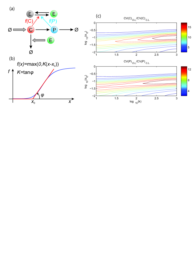
Figure 4: (a) The SFE network with feedback (two possible configurations). (b) Red line: the class of feedback functions considered in this work, which can approximate a Hill function around its lower end. (c) Ratio of open-loop vs. closed-loop CVs as a function of $\alpha_{E}$ (which determines the average number of active enzymes) and $k$ for $K=3,~{}C_{0}=5,~{}N=10,~{}\mu_{E}=0.1,~{}\alpha_{C}=5010,~{}\nu=1,~{}\mu_{P}=1$.

In the following we analyze the closed-loop SFE network behavior by studying how the SFE network properties described in the previous sections are transformed under feedback.

2.2.1 Feedback results in a dramatic noise reduction and increased robustness to parameter variation

Here we study the SFE network under the influence of negative feedback. We should point out that we characterize the open- and closed-loop systems with respect to the same features (noise and robustness), not to directly compare them, but because these features play an important role in the function of both mechanisms. Whenever we use the open-loop system as a baseline for assessing closed-loop system properties, scale-independent measures are used since this allows for the evaluation of relative distribution spreads. This principle is only disregarded in Fig. 5 below.

For our first test, we use the same settings and parameters as those of Fig. 2(a), only this time we add a feedback term from the substrate to the enzyme activation rate. Increasing the gain $K$ or shifting the activation point $x_{0}$ to the left results in a decrease of both means and variances of substrate and product. For the ranges of $K$ and $x_{0}$ values considered, the means change by at most a factor of 2.5, while the variances by about 5 times. At the same time, the CVs vary by about 50% and the corresponding Fano Factors by a factor of 5. Moreover, as the analysis in the Supplement (section 5) shows, the CVs of both species become relatively flat as $K$ and $x_{0}$ increase, while the Fano Factor gets very close to 1 as $K$ increases for small values of $x_{0}$, indicating that the resulting substrate and product stationary distributions are approximately Poissonian in this regime. For the analysis that follows, we fix $K=3$ and $x_{0}=5$ in the feedback function $f(\cdot)$.

With the above choice of feedback parameters, we first study the sensitivity of the closed-loop SFE system to variations of the two key parameters, $\alpha_{E}$ and $k$. As Fig. 2(b) demonstrates, means and variances (and, consequently, CVs) of substrate and product become largely independent of $\alpha_{E}$, except for very large values of $k$ (similar results are obtained for product feedback). Moreover, noise of substrate and product is dramatically reduced in comparison to the open-loop SFE system, while the variation of means and variances is now quite small, despite the large ranges of $\alpha_{E}$ and $k$ values considered. It is also worth noting that the Fano Factors of both substrate and product are very close to one for a large range of parameters.

Interestingly, if we quantify noise reduction by the ratio of open-loop vs. closed-loop CV, we observe that noise reduction is maximal where the open-loop SFE system noise is greatest, as demonstrated by comparing Fig. 4(c) with Fig. 2(a).

Another striking effect of feedback regulation of enzyme activity is that the closed-loop SFE system becomes much less sensitive to parameter variations in comparison to the open-loop case. Applying the same parametric perturbations described in §2.1.3, we obtain the histograms of Fig. 3 (continuous lines). As it becomes apparent, the histograms corresponding to the closed-loop SFE system are several orders of magnitude narrower compared to the open-loop. Moreover, despite the relatively large parametric perturbations, variability in substrate and product statistics of the closed-loop SFE system is largely contained within an order of magnitude.

As it was pointed out in §2.1.3, variability in biochemical reaction rates can be considered “artificial”, however changes in the number of enzymes, $N$, are to be expected in a cellular population. It is therefore interesting to study how variations in $N$ alone are propagated to the substrate and product statistics. Assuming that both the open- and closed-loop systems operate with the same average number of active enzymes for the “nominal” value of $N=8$, Fig. 5(a,b) shows how the substrate mean and variance vary as $N$ is perturbed around this value, both in the open- and closed-loop systems (with substrate feedback). To achieve the same average number of active enzymes for $N=8$, the closed-loop SFE system was simulated first, and the mean number of active enzymes was recorded. This number was then used to back-calculate an appropriate $\alpha_{E}$ value (keeping $\mu_{E}$ fixed) for the open-loop SFE system. Panel (c) also shows how the distribution of active enzymes differs in the two systems for $N=8$. The cyan line corresponds to a binomial distribution, $\mbox{B}(8,p)$, where $p=\alpha_{E}/(\alpha_{E}+\mu_{E})$ is determined by the $\alpha_{E}$ and $\mu_{E}$ values of the open loop. The red distribution is obtained from simulation of the closed loop and is markedly different from a binomial. The difference is especially significant at the lower end, as small values of $E^{*}$ lead to fast accumulation of $C$. Similar results are obtained for product feedback.

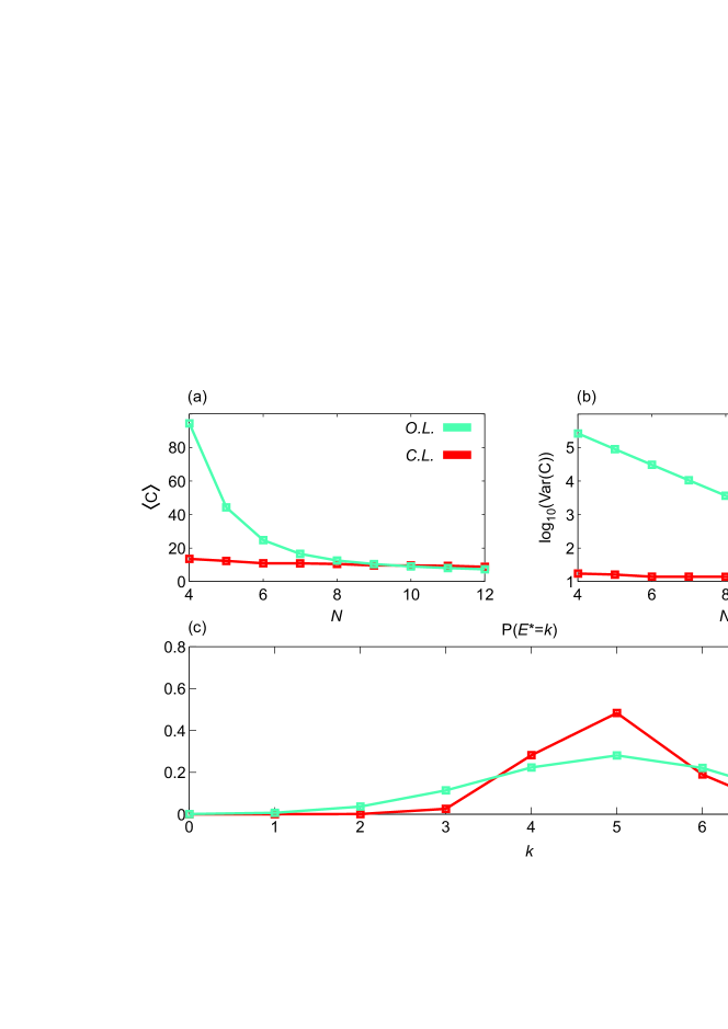
Figure 5: (a, b) Mean and variance of substrate in the open- and closed-loop SFE system with substrate feedback (notice the logarithmic variance scale). The closed loop was simulated with $\alpha_{E}=0.04$, $\mu_{E}=0.1$, $\alpha_{C}=5010$, $\nu=1$, $k=100$, $\mu_{P}=1$ and feedback parameters $K=10$, $C_{0}=15$. In the open-loop SFE system all parameters were kept the same, except for $\alpha_{E}$, which was set to 0.1572 to achieve the same mean of $E^{*}$ that the closed-loop SFE system achieves for $N=8$.

2.2.2 Open-loop stochasticity vs. closed-loop determinism

A further remarkable by-product of feedback in the closed-loop SFE system is the fact that the mean of the stochastic model ends up following very closely the predictions of the ODE equations for the deterministic system. This behavior becomes more pronounced as the number of available enzymes ($N$) grows, while the average number of active enzymes ($N\alpha_{E}/(\alpha_{E}+\mu_{E})$) remains small. Under this condition, one can think of enzyme activation in the original system as a zeroth-order reaction with rate $N\alpha_{E}$, and the active enzyme abundance to be described by a birth-death process with birth rate $N\alpha_{E}$, death rate $\mu_{E}$ and Poisson stationary distribution with parameter $\lambda=N\alpha_{E}/\mu_{E}$.

The accuracy of the ODE approximation to the mean substrate levels in the case of substrate feedback can be demonstrated using the same type of parametric perturbations with those employed in §2.1.3. All nominal parameters were kept the same for this test, except for $\mu_{E}$, $N\alpha_{E}$ and $k$, which were set equal to 1, 5 and 100 respectively ($N=100$, $\alpha_{E}=0.05$). We compare the mean of the stochastic model with the ODE prediction in the case of substrate feedback with $K=0.4,~{}x_{0}=5$, and define the relative error

$$R.E. :=\frac{|\langle C\rangle-C_{ss}|}{\langle C\rangle}\cdot 100\%,$$ (2)

where $C_{ss}$ is the equilibrium solution of the ODE model. In this setting, a set of 5000 random perturbations leads to an average relative error of 1.5% with standard deviation 0.96%, which clearly shows that the ODE solution captures the mean substrate abundance with very good accuracy indeed (note that the same holds for the mean of $P$, since it depends linearly on the mean of $C$). Very similar results are obtained in the case of product feedback.

The above observations are even more striking, if we take into account 1) the fact that the closed-loop SFE system is still highly nonlinear and 2) the intrinsic property of stochastically focused systems to display completely different mean dynamics when compared to the ODE solutions. An explanation of this behavior can be given by examining the moment differential equations. In the limiting case considered in this section, denoting $\alpha_{E}(C)$ the production rate of active enzyme, we obtain

$$\frac{d\langle C\rangle}{dt} =\alpha_{C}-\nu\langle C\rangle-k\langle E^{*}C\rangle=\alpha_{C}-\nu\langle C\rangle-k\mbox{Cov}(E^{*},C)-k\langle C\rangle\langle E^{*}\rangle$$ (3)

$$\frac{d\mbox{Cov}(E^{*},C)}{dt} =-(\mu_{E}+\nu)\mbox{Cov}(E^{*},C)-\mbox{Cov}(kE^{*}C,E^{*})+\mbox{Cov}(\alpha_{E}(C),C)$$ (4)

The last two terms on the right-hand side of (4) denote the covariance of the substrate enzymatic degradation rate with active enzyme and the covariance of the enzyme activation rate with the substrate. Both covariances are expected to be positive at steady state, which implies that the terms act against each other in determining the steady-state covariance of substrate and active enzyme. In turn, a small value of this covariance (compared to the product $\langle C\rangle\langle E^{*}\rangle$) implies that the mean of $C$ can be approximately captured by a mean-field equation, where $\langle E^{*}C\rangle$ has been replaced by $\langle C\rangle\langle E^{*}\rangle$. This is indeed the case in our simulations, where $\mbox{Cov}(E^{*},C)$ turns out to be $\sim$20–30 times smaller than $\langle C\rangle\langle E^{*}\rangle$. On the other hand, the open-loop value of $\mbox{Cov}(E^{*},C)$ is about 30 times larger than the closed-loop one. This comes as no surprise, as one expects substrate and active enzyme to display a strong negative correlation, which is the cause of the discrepancy between stochastic and deterministic descriptions of stochastically focused systems.

Similar observations can be made when $N$ is small (e.g. around 10), however the relative errors become at least one order of magnitude larger. We believe that this can be attributed to the fact that the enzyme activation propensity depends both on the abundance of inactive enzyme and the substrate/product abundance, which increases the inaccuracy of the ODEs.

2.2.3 The feedback mechanism is intrinsically robust

As we have already demonstrated, the closed-loop SFE system is remarkably robust to parametric perturbations of the open-loop model. However, in all of our numerical experiments we have kept the parameters of the feedback function $f$ fixed to a few different values. Here we examine the opposite situation, in which only the controller parameters are free to vary while the rest are held constant. We therefore consider the problem of regulating the mean of $C$ around a fixed value with feedback from $C$. The problem can be posed as follows:

$$\underset{K,~{}C_{0}}{\min}~{}~{}h(K,~{}C_{0}):=\langle(C-C_{target})^{2}\rangle=(\langle C\rangle_{ss}-C_{target})^{2}+\mbox{Var}(C)_{ss},$$

where both the mean and variance of $C$ depend on the feedback function parameters. Fig. 6 shows the contour lines of $h$, obtained via stochastic simulation over a wide range of $K$ and $C_{0}$ values for $C_{target}=10$. It can be observed that $h$ is more sensitive to $C_{0}$ than $K$: beyond a certain $K$ value, the function quickly levels off.

Based on our simulation runs, the optimal feedback parameters turned out to be $K=30$ (the maximum $K$ value considered for the plot) and $C_{0}\simeq 16$ (given the inevitable uncertainty in $h$ due to sampling variability, the true optimal value should be close to this). The optimal feedback function therefore resembles a “barrier”: for $x<C_{0}$ it is zero, while it rises very steeply beyond $C_{0}$.

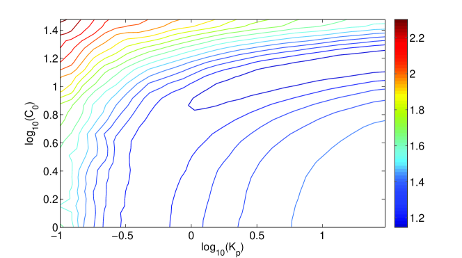
Figure 6: Contour lines of $\log_{10}(h(K,C_{0}))$ for $C_{target}=10$, obtained by evaluating the function via stochastic simulation on a logarithmic grid in the parameter space.

Note that the mean and variance of $C$ both depend on $(K,C_{0})$, but neither quantity is available in closed form as a function of the feedback parameters or obtainable from a closed set of moment equations. Thus, $h$ had to be evaluated on a grid with the help of stochastic simulation. Alternatively, as we show in the Supplement (section 6), one can exploit the behavior presented in the previous Section, and optimize a similar objective function by directly evaluating the required moments of $C$ using a simple moment closure approximation based on the method of moments. This scheme, introduced in [10], provides very accurate approximations of the mean and variance at a fraction of the computational effort, thus allowing optimization to be carried out very efficiently. The optimal parameters for the approximate system can be used as starting points in the optimization of $h$.

3 Discussion

In this work we have examined the behavior of a branched enzymatic reaction scheme. This system has already been shown to display stochastic focusing, a sensitivity amplification phenomenon that arises due to nonlinearities and stochasticity whenever only a few enzyme molecules are present in the system. We have additionally shown that when the enzyme activity evolves on a slow timescale compared to that of the substrate, very large fluctuations can be generated in the system. Moreover, the dynamics of the system is extremely sensitive to variations in its reaction rates. Both these observations imply that this simple model is not appropriate for robust signal detection.

We asked how the system behavior would change in the presence of a feedback mechanism, so that the “controller” molecule ($E^{*}$) could sense the fluctuations in $C$ (its substrate) or $P$ (the product of the alternative reaction branch). We have shown that noise decreases dramatically in the presence of feedback, while the robustness of the average system behavior is boosted significantly. Consequently, the focused system with feedback ends up behaving almost as predictably as a mean-field ODE model, even when the number of active enzymes is very small.

There exist several biochemical systems which in certain aspects match the main ideas behind the SFE motif, i.e. display stochastic fluctuations in enzyme activity/abundance and substrate/product feedback activation. For example, it was recently discovered [16] that the guanine nucleotide exchange factor SOS and its substrate, the Ras GTPase, are involved in a feedback loop where SOS converts Ras-GDP (inactive) to Ras-GTP (active) and, in turn, active Ras allosterically stabilizes the high-activity state of SOS. Another prominent example is microRNA post-transcriptional regulation of gene expression [34], where a microRNA may mediate the degradation of a target mRNA, while the protein arising from this mRNA in turn activates the microRNA transcription.

Yet another instance is the heat shock response system in E. coli [8]: here the $\sigma^{32}$ factor, which activates the heat-shock responsive genes, is quickly turned over under the action of the protease FtsH at normal growth temperatures. After a shift to high temperature, $\sigma^{32}$ is rapidly stabilized and at the same time it also activates the synthesis of FtsH. The FtsH-mediated degradation of $\sigma^{32}$ is under negative feedback. Finally, it is known that mRNA decapping (a process that triggers mRNA degradation) is controlled by the decapping enzyme Dcp2, which fluctuates between an open (inactive) and closed (active) form. Experimental evidence suggests that the closed conformation of the enzyme is promoted by the activator protein Dcp1 together with the mRNA substrate itself [12, 5]. We should stress, however, that it is still unclear if any of the aforementioned examples display all the dynamic features of the motif considered in this work. Speaking generally, due to the required levels of measurement accuracy, it is difficult to find examples that exactly match the conditions considered here with current experimental techniques. However, it is certainly conceivable that this will be achieved in the future.

An interesting feature of our system is that homeostasis is achieved with a very small number of controller molecules (in the order of 10), which are able to maintain the output at a very low level with fluctuations that are – to a good approximation – Poissonian. We have considered two alternative feedback schemes: in the first the substrate directly affects the activation rate of the enzyme (a case of substrate activation), while in the second the product of the alternative reaction branch is used as a “proxy” for the substrate abundance. Note that the flux through the $C$-$P$ branch is many orders of magnitude smaller than the flux in the $E$-regulated branch. The $C$-$P$ branch can thus be thought to act as a “sensor mechanism”, used to control the high-flux branch of the system. To the best of our knowledge, this type of feedback has not yet been observed in naturally occurring reactions.

Finally, it is worth to note that one could achieve this type of regulation with an “unfocused” system, in which the coupling between enzyme and substrate (parameter $k$) would be much smaller. This would imply, however, that the number of enzyme molecules needed to achieve the same substrate levels would have to be much greater, and this could entail an added cost for a living cell.

In summary, to regulate a low-copy, high-flux substrate via an enzymatic mechanism such as the one considered here, there are three possibilities: a) use of a low number of controller enzymes and strong coupling between enzyme and substrate (which results in stochastic focusing and noise), b) use of a high-copy enzyme and weak coupling (with the associated production cost) or c) use of a low-copy controller with feedback: an alternative which, as we have demonstrated, leads to a remarkably well-behaved closed-loop system.

It is thus conceivable that cellular feedback mechanisms have evolved to exploit the nature of stochastically focused systems to achieve regulation of low-copy substrates with the minimal number of controller molecules. We expect that the rapid development of experimental techniques in single-molecule enzymatics will soon enable the experimental verification of our findings and possibly the discovery of similar noise attenuation mechanisms inside cells. Finally, our results can be seen as a first step towards the rational manipulation of noise properties in low-copy enzymatic reactions.

Stochastic focusing coupled with negative feedback enables robust regulation in biochemical reaction networks:
Supplementary Material

Appendix A Some comments on the choice of the reaction scheme

A.1 Theoretical analysis

The main point of our analysis here is to determine the sensitivity of a branched-reaction product to changes in the activation rate of an enzyme and in this way provide some justification for our modeling choices. The rationale behind this analysis is that one cannot hope to control the mean - let alone the variance - of a product, if its statistics are not sensitive to changes in the enzyme. With this in mind, we examine the following branched reaction system:

$$\varnothing\displaystyle\mathrel{\mathop{\vbox{ \hbox{ \ooalign{\raise 1.0pt\hbox{$\relbar\joinrel\rightharpoonup\joinrel$}\crcr\lower 1.0pt\hbox{$\leftharpoondown\joinrel\relbar\joinrel$}} } }}^{\alpha_{E}\mathstrut}_{\mu_{E}}}E$$

$$\varnothing\xrightarrow{\alpha_{C}}C$$

$$C\xrightarrow{\nu}P\xrightarrow{\mu_{P}}\varnothing$$

$$C+E\xrightarrow{k}Q+E$$

$$Q\xrightarrow{\mu_{Q}}\varnothing$$

The system consists of the following:

• An enzyme $E$, that is found in low copy numbers and therefore its fluctuations have a significant impact on system behavior.

• A high-copy, low-noise enzyme (not shown), responsible for the conversion of $C$ to $P$. Alternatively, we can assume that $C$ “matures” into $P$ without the help of an enzyme. In both cases, this reaction can be considered to be first-order, even if it is enzymatic.

• Two products, $P$ and $Q$, which are produced from $C$

• The substrate species, $C$, which plays the most critical role. $C$ enters the system through a zeroth-order reaction, and can have two alternate fates: it can either be converted to $P$ or $Q$.

The initial sensitivity question can be now posed more precisely: which of the two reaction products, $P$ or $Q$, is more sensitive to changes in the activation rate of $E$? Apart from the system structure, we are making the following assumptions regarding the reaction rates:

• The bimolecular reaction rate ($k$) is large compared to the first-order reaction rate of $C$ ($\nu$). That is, most of the influx of $C$ is directed towards $Q$. This assumption amplifies the effect of the nonlinear kinetics in the system (in the opposite case, the bimolecular reaction could be considered as a perturbation in an almost-linear network).

• The influx of $C$ to the system is high, i.e. $\alpha_{C}$ is also large.

• The rates of $E$ are such that $E$ has low copies and high noise (this was already stated above), so that we cannot replace $E$ by its mean in the bimolecular reaction.

We now want to see what happens to the steady-state means $\langle P\rangle_{ss}$ and $\langle Q\rangle_{ss}$ when $\alpha_{E}$ varies. In the case of $\langle P\rangle_{ss}$, the situation is simple: $\langle P\rangle_{ss}$ follows the behavior of $\langle C\rangle_{ss}$,

$$\langle P\rangle_{ss}=\frac{\nu}{\mu_{P}}\langle C\rangle_{ss}.$$

Thus, our focus shifts from $P$ to $C$ in this case. If the mean of $C$ is sensitive to changes in $E$, we know that $P$ will be sensitive as well. This is precisely the case when stochastic focusing is present.

In the case of $Q$, the situation is different: we expect it to be so, because in order to produce a $Q$ molecule, we need both $E$ and $C$ to be present. Therefore, if $E$ hits zero, $C$ will inevitably accumulate (since we assumed that the rate of the alternate path, $\nu$, is small), but no $Q$ will be produced. Instead, while $E$ stays at zero, $Q$ will drop with a speed that depends on $\mu_{Q}$. Once $E$ returns to non-zero numbers, the accumulated amount of $C$ will be converted into $Q$ in a strong production burst. Depending on $\mu_{Q}$, this may result in a brief burst of $Q$, or may go unnoticed (when $\mu_{Q}$ is small enough, the burst will happen, because $Q$ cannot be removed fast enough from the system). We thus see that $Q$ can display a more complex behavior than $P$.

We next turn to the mean of $Q$. Since $\nu\ll k$, let us assume first that $\nu\simeq 0$. In this case, the first-moment equation for $C$ will give

$$\langle EC\rangle_{ss}=\frac{\alpha_{C}}{k}.$$

Note that the mean of $C$ does not appear there, because we assumed no first-order degradation. The equation says that the steady-state mean of the product of $E$ with $C$ is constant, independently of $\alpha_{E}$. Turning to the equation of the first moment of $Q$, we then get

$$\langle Q\rangle_{ss}=k\frac{\langle EC\rangle_{ss}}{\mu_{Q}}=\frac{k\alpha_{C}}{k\mu_{Q}}=\frac{\alpha_{C}}{\mu_{Q}},$$

which shows that $Q$ is also not affected in its mean by changes in the rates of $E$. Intuitively, we can see why it is plausible for the mean of $Q$ to remain constant, by looking at the bimolecular reaction that produces it: when $\alpha_{E}$ increases, the mean of $C$ drops and vice versa. Thus, the average production rate of $Q$ cannot change that much — and in fact, does not change at all in the limiting case $\nu=0$.

Using this observation, we can understand also why $\langle Q\rangle_{ss}$ is not sensitive to $\alpha_{E}$ when $\nu$ is non-zero but small: while in this case the above relations do not hold exactly, we still expect them to hold with good precision (simulation verifies that). Overall then, we see that $Q$ is relatively insensitive to changes in $\alpha_{E}$, compared to $P$, and it makes sense to consider $Q$ as the target for regulation.

It should be noted that the above arguments hold only for the means of $P$ and $Q$. We do not expect the variance of $Q$ to be equally insensitive to the noise in $E$, however it is not entirely clear how $Q$ could be used in a noise-suppressing feedback mechanism.

A.2 Numerical verification

A.2.1 The sensitivity of $Q$

To get a feeling for the scaling of the different constants we consider the equilibrium solutions to the ODE model of the network. The following three relations are immediate:

$$C_{ss} =\frac{\alpha_{C}}{\nu+kE_{ss}},$$ (5)

$$E_{ss} =\frac{\alpha_{E}}{\mu_{E}},$$ (6)

$$Q_{ss} =\frac{kC_{ss}E_{ss}}{\mu_{Q}}.$$ (7)

Assuming the mean lifetime of the substrate and the enzyme to be about the same we may pick the units of time such that $\mu_{C}=\mu_{E}=1$. As we are interested in stochastic focusing, a low copy-number phenomenon, we further prescribe as a base case that $C_{ss}=E_{ss}=Q_{ss}=10$. Combined with (5) and (7) this implies

$$\alpha_{C} =10\cdot(1+10k),$$ (8)

$$\mu_{Q} =10k.$$ (9)

With the enzymatic rate parameter $k$ still free and (8)–(9) given, we can next consider the rate for the inflow of enzyme $\alpha_{E}$ to be an adjustable parameter which controls the amount of product $Q$.

Using (5)–(7) and (8)–(9) we arrive at the relation

$$Q_{ss} =\alpha_{E}\frac{1+10k}{1+\alpha_{E}k}.$$ (10)

For any given rate $k$ and desirable setpoint $Q_{set}$, (10) can be solved for the value of $\alpha_{E}$ that makes $Q_{ss}=Q_{set}$.

We now define the gain $g$ as the response to a 50% decrease of enzyme from the base case $\alpha_{E}=10$,

$$g=Q_{ss}(\alpha_{E}=10)/Q_{ss}(\alpha_{E}=5)-1.$$ (11)

With $g\leq 0$, $Q$ does not respond (i.e. is insensitive), and $g=1=10/5-1$ can be considered a perfect transmission.

In the table below values from (11) using (10) have been computed for different values of the rate constant $k$. The conclusion is that $k\lesssim 1$ is required for the network to be responsive.

$k$	$10^{-2}$	$10^{-1}$	$10^{0}$	$10^{1}$	$10^{2}$
$Q_{ss}(\alpha_{E}=10)$	10	10	10	10	10
$Q_{ss}(\alpha_{E}=5)$	5.24	6.67	9.17	9.90	9.99
$g$	0.9091	0.5000	0.0909	0.0099	0.0010

In the stochastic setting, we note that focusing occurs due to a large rate constant $k\gg 1$ since this is the only nonlinearity present in the model. The following numerical results were obtained after averaging over 5000 trajectories.

$k$	$10^{-2}$	$10^{-1}$	$10^{0}$	$10^{1}$	$10^{2}$
$\langle Q\rangle_{\alpha_{E}=10}$	$10.01\pm 3.04$	$9.85\pm 3.40$	$9.91\pm 3.25$	$9.99\pm 3.18$	$10.00\pm 3.17$
$\langle Q\rangle_{\alpha_{E}=5}$	$7.13\pm 2.48$	$6.53\pm 2.967$	$8.91\pm 3.44$	$9.84\pm 3.44$	$9.97\pm 4.02$
$g$	0.4039	0.5087	0.1113	0.0152	0.0028

The conclusion is that neither the deterministic nor the stochastic model of $Q$ is sensitive to changes in the enzyme when focusing is present.

A.2.2 The sensitivity of $P$

As before we pick units of time such that $\mu_{E}=\nu=1$. We get from the ODE equilibrium solutions that

$$C_{ss} =\frac{\alpha_{C}}{\nu+kE_{ss}}$$ (12)

$$E_{ss} =\frac{\alpha_{E}}{\mu_{E}}$$ (13)

$$P_{ss} =\frac{\nu C_{ss}}{\mu_{P}},$$ (14)

such that via the base case $C_{ss}=E_{ss}=P_{ss}=10$ we arrive at

$$\alpha_{C} =10\cdot(\nu+10k),$$ (15)

$$\mu_{P} =\nu.$$ (16)

We now define the gain $g$ as

$$g=\langle P\rangle_{\alpha_{E}=5}/\langle P\rangle_{\alpha_{E}=10}-1$$ (17)

since the enzyme $E$ this time acts as an inhibitor. In the table below we compute the gain for various values of $\nu$ with $k=10^{2}$. It can be seen that, in the deterministic case, this network has good transmission ($g\sim 1$) when $\nu\lesssim k$.

$k$	$10^{2}$	$10^{2}$	$10^{2}$	$10^{2}$	$10^{2}$
$\nu$	$10^{-1}$	$10^{0}$	$10^{1}$	$10^{2}$	$10^{3}$
$g$	1	1	0.98	0.83	0.33

In the stochastic regime we performed many simulations for various combinations of parameters $k$ and $\nu$. The table below summarizes the most interesting results found in this way. The stochastic focusing effect is clearly present in the observed increase of gain compared to the deterministic model.

$k$	$10^{2}$	$10^{2}$	$10^{2}$	$10^{2}$
$\nu$	$10^{-1}$	$10^{0}$	$10^{1}$	$10^{2}$
$\langle P\rangle_{\alpha_{E}=10}$	$10.65\pm 3.39$	$11.32\pm 5.31$	$11.31\pm 3.25$	$11.01\pm 5.18$
$\langle P\rangle_{\alpha_{E}=5}$	$22.41\pm 32.49$	$36.08\pm 92.08$	$29.42\pm 53.49$	$21.80\pm 12.61$
$g$	1.2410	2.6080	1.9420	1.1800

Appendix B Considering the effect of enzyme saturation in the catalytic degradation reaction

We here consider a more realistic enzymatic reaction mechanism for the degradation of the substrate $C$, which includes the formation of an enzyme-substrate complex. As we will see, this more detailed mechanism implies an overall behavior which is similar to the SFE model studied in the main paper

The mechanism is displayed on Fig. 7. According to this scheme, active enzyme ($E*$) and substrate have to first form a complex before $C$ is degraded. If the enzyme spontaneously switches to its inactive form while bound to $C$, we assume that the complex dissociates.

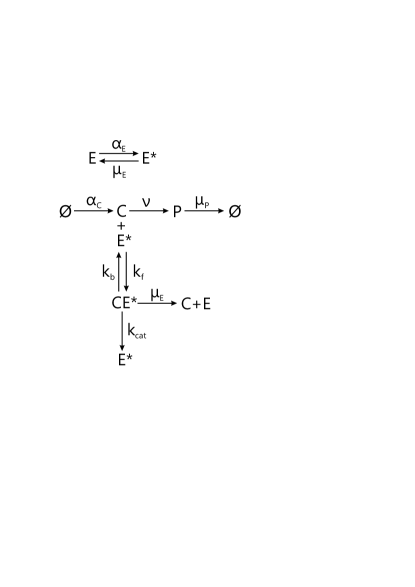
Figure 7: A more detailed reaction mechanism for substrate degradation.

With the additional reactions, the open-loop system becomes again analytically intractable, as the conditional moment equations are no longer closed. We will therefore base our analysis on the behavior of the corresponding deterministic system. To further simplify the task, we will first assume a fixed number of active enzymes, $E^{*}_{tot}=E^{*}+CE^{*}$, i.e. ignore the enzyme (de)activation reactions. Moreover, we will assume that the substrate flux towards $P$ is much smaller than the flux into the enzymatic reaction and therefore set $\nu=0$. Under these conditions, one can verify that the steady-state concentration of substrate and free (active) enzyme are given by the following expressions:

$$C_{ss} =\frac{\alpha_{C}(k_{b}+k_{cat})}{k_{f}(k_{cat}E^{*}_{tot}-\alpha_{C})}$$ (18)

$$E^{*}_{ss} =\frac{k_{cat}E^{*}_{tot}-\alpha_{C}}{k_{cat}}$$ (19)

We see that the existence of a finite positive steady-state for the system depends on the relation of $E^{*}_{tot}$ with the ratio $\alpha_{C}/k_{cat}$, which connects the rates of substrate influx and the catalytic efficiency of the active enzyme. In other words, if there is not a sufficient number of active enzymes in the system, there is no finite and positive steady-state; instead, the number of substrate molecules tends to infinity, as the existing free enzyme molecules are completely saturated and cannot process all incoming substrate molecules.

When an alternative fate is available for the substrate (e.g. its conversion to $P$), the system will of course be stable, as the alternative pathway will absorb the excess substrate. However, if $\nu$ is small compared to $k_{cat}$, the resulting steady-state substrate concentration, expected to be close to $\alpha_{C}/\nu$, will be large.

Now, let us consider the case where $E^{*}_{tot}$ is varied externally. As it approaches $\alpha_{C}/k_{cat}$ from above, the steady-state concentration of $C$ quickly diverges to infinity. Therefore, it is reasonable to imagine that if active enzymes fluctuate slowly, randomly and close to the critical value $\alpha_{C}/k_{cat}$, this will result in dramatic fluctuations in $C$.

The intuition obtained from the above observations is confirmed by stochastic simulation of the system, as shown on Fig. 8.

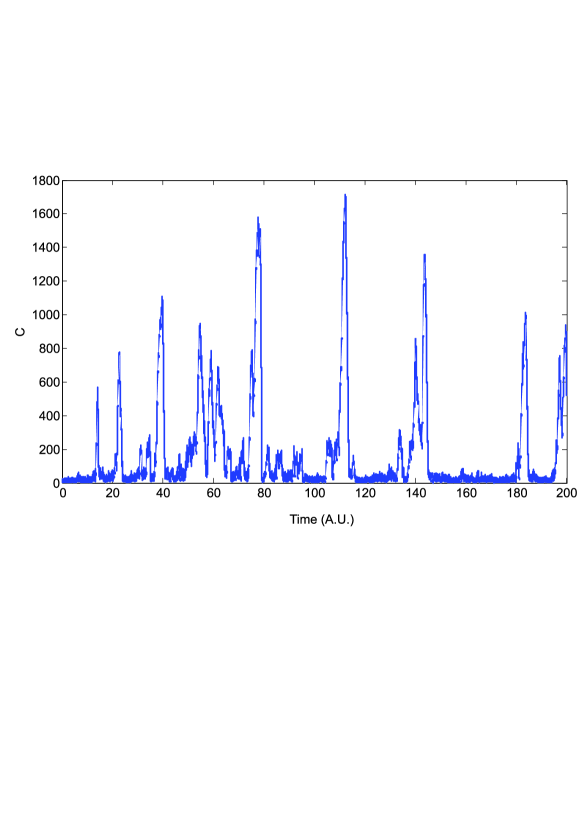
Figure 8: A sample path of $C$ for the system of Fig. 7 for $\alpha_{E}=0.16$, $\mu_{E}=0.1$, $\alpha_{C}=5000$, $\nu=1$, $\mu_{P}=1$, $k_{f}=100$, $k_{b}=10$, $k_{cat}=1000$ and $N=10$ ($N$ is the total number of enzymes, as defined previously). With the selected rates the average number of active enzymes is close to 6, while $\alpha_{C}/k_{cat}=5$. As expected, we observe an amplification of the enzyme fluctuations in the substrate abundance.

In summary, the open-loop SFE network with the more detailed enzymatic reaction mechanism displays a behavior analogous to the simplified system considered in the main paper, with the only difference that when enzyme saturation is taken into account even a non-zero number active enzymes may be insufficient to prevent large substrate fluctuations, if the enzyme is not much faster compared to the rate of substrate influx (i.e. $k_{cat}\gg\alpha_{C}$).

Provided the total number of available enzymes is greater than the necessary minimum to prevent complete saturation, we expect that addition of feedback from $C$ or $P$ to the enzyme will, similarly to the simplified case, result in great noise reduction. For the example presented on Fig. 8, the CV of $C$ was reduced from about 2 to about 0.38 and the Fano Factor from about 900 to about 1.73 for $K=50$ and $C_{0}=20$. Remarkably, the steady-state means of the system were again very close to the ODE steady-state (obtained from numerical simulation of the deterministic system): $\langle C\rangle_{ss}\approx 11.5$, $\langle E^{*}\rangle_{ss}\approx 4.6$ and $\langle E\rangle_{ss}=0.4$, whereas $C_{ss}=10.52$, $E^{*}_{ss}=4.78$ and $E_{ss}=0.22$.

Appendix C Conditional moment equations for the open-loop system

Denote $E^{*}$ by $Y$, $C$ by $Z_{1}$ and $P$ by $Z_{2}$. Since the total number of enzymes, $E+E^{*}$ is assumed equal to $N$, we can write the dynamics of $E^{*}$ without reference to $E$:

$$\varnothing\xrightarrow{\alpha_{E}(N-E)}E\xrightarrow{\mu_{E}}\varnothing.$$

We also know that the stationary distribution of $E^{*}$ is $\mbox{B}(N,p)$, where $p=\frac{\alpha_{E}}{\alpha_{E}+\mu_{E}}$. We can thus describe the evolution of moments of $C$ conditioned on the state of $E^{*}$, following the approach described in [3]. We further simplify the problem by considering the steady-state conditional moments. Following the notational conventions of [3], we set

$$\lim_{t\to\infty}\mathbb{E}[Z_{1}|y,t]:={\color[rgb]{1,0,0}\mu_{1}(y)}$$

$$\lim_{t\to\infty}\mathbb{E}[Z_{2}|y,t]:={\color[rgb]{1,.5,0}\mu_{2}(y)}$$

$$\lim_{t\to\infty}\mathbb{E}[\left(Z_{1}-{\color[rgb]{1,0,0}\mu_{1}(y,t)}\right)^{2}|y,t]:={\color[rgb]{0,0,1}C_{(2,0)}(y)}$$

$$\lim_{t\to\infty}\mathbb{E}[\left(Z_{2}-{\color[rgb]{1,.5,0}\mu_{2}(y,t)}\right)^{2}|y,t]:={\color[rgb]{1,0,1}C_{(0,2)}(y)}$$

$$\lim_{t\to\infty}\mathbb{E}[\left(Z_{1}-{\color[rgb]{1,0,0}\mu_{1}(y,t)}\right)\left(Z_{2}-{\color[rgb]{1,.5,0}\mu_{2}(y,t)}\right)^{2}|y,t]:={\color[rgb]{0,.5,.5}C_{(1,1)}(y)}$$

$$\lim_{t\to\infty}\mathbb{P}[Y(t)=y]:=p(y)$$

The steady-state first- and second-order conditional moments of $C$ and $P$ are then obtained by solving the following system of linear equations:

$$\mbox{\bf Steady-state equation for }{\color[rgb]{1,0,0}\mu_{1}(y)}:$$

$$\alpha_{C}p(y)-{\color[rgb]{1,0,0}\mu_{1}(y)}p(y)\left(\alpha_{E}(N-y)+\mu_{E}y+\nu+ky\right)+\alpha_{E}(N-y+1){\color[rgb]{1,0,0}\mu_{1}(y-1)}p(y-1)+$$

$$+\mu_{E}(y+1){\color[rgb]{1,0,0}\mu_{1}(y+1)}p(y+1)=0$$ (20)

$$\mbox{\bf Steady-state equation for }{\color[rgb]{1,.5,0}{\color[rgb]{1,.5,0}\mu_{2}(y)}}:$$

$$\nu{\color[rgb]{1,0,0}\mu_{1}(y)}(y)p(y)-{\color[rgb]{1,.5,0}{\color[rgb]{1,.5,0}\mu_{2}(y)}}p(y)\left(\alpha_{E}(N-y)+\mu_{E}y+\mu_{P}\right)+\alpha_{E}(N-y+1){\color[rgb]{1,.5,0}\mu_{2}(y-1)}p(y-1)+$$

$$\mu_{E}(y+1){\color[rgb]{1,.5,0}\mu_{2}(y+1)}p(y+1)=0$$ (21)

$$\mbox{\bf Steady-state equation for }{\color[rgb]{0,0,1}C_{(2,0)}(y)}:$$

$$\alpha_{C}p(y)+\alpha_{E}(N-y+1)\left({\color[rgb]{1,0,0}\mu_{1}(y-1)}-{\color[rgb]{1,0,0}\mu_{1}(y)}\right)^{2}p(y-1)+\mu_{E}(y+1)\left({\color[rgb]{1,0,0}\mu_{1}(y-1)}-{\color[rgb]{1,0,0}\mu_{1}(y)}\right)^{2}p(y+1)+$$

$$+\nu{\color[rgb]{1,0,0}\mu_{1}(y)}p(y)+ky{\color[rgb]{1,0,0}\mu_{1}(y)}p(y)-{\color[rgb]{0,0,1}C_{(2,0)}(y)}p(y)\left(\alpha_{E}(N-y)+\mu_{E}y+2ky+2\nu\right)+$$

$$+\mu_{E}(y+1){\color[rgb]{0,0,1}C_{(2,0)}(y+1)}p(y+1)+\alpha_{E}(N-y+1){\color[rgb]{0,0,1}C_{(2,0)}(y-1)}p(y-1)=0$$ (22)

$$\mbox{\bf Steady-state equation for }{\color[rgb]{1,0,1}C_{(0,2)}(y)}:$$

$$\alpha_{E}(N-y+1)\left({\color[rgb]{1,.5,0}\mu_{2}(y-1)}-{\color[rgb]{1,.5,0}\mu_{2}(y)}\right)^{2}+\mu_{E}(y+1)\left({\color[rgb]{1,.5,0}\mu_{2}(y+1)}-{\color[rgb]{1,.5,0}\mu_{2}(y)}\right)^{2}+\nu{\color[rgb]{1,0,0}\mu_{1}(y)}p(y)+$$

$$+\mu_{P}{\color[rgb]{1,.5,0}\mu_{2}(y)}p(y)-{\color[rgb]{1,0,1}C_{(0,2)}(y)}p(y)\left(\alpha_{E}(N-y)+\mu_{E}y+2\mu_{P}\right)+\mu_{E}(y+1){\color[rgb]{1,0,1}C_{(0,2)}(y+1)}p(y+1)+$$

$$+\alpha_{E}(N-y+1){\color[rgb]{1,0,1}C_{(0,2)}(y-1)}p(y-1)+2\nu{\color[rgb]{0,.5,.5}C_{(1,1)}(y)}p(y)=0$$ (23)

$$\mbox{\bf Steady-state equation for }{\color[rgb]{0,.5,.5}C_{(1,1)}(y)}:$$

$$\alpha_{E}(N-y+1)\left({\color[rgb]{1,0,0}\mu_{1}(y-1)}-{\color[rgb]{1,0,0}\mu_{1}(y)}\right)\left({\color[rgb]{1,0,0}\mu_{2}(y-1)}-{\color[rgb]{1,0,0}\mu_{2}(y)}\right)p(y-1)+$$

$$+\mu_{E}(y+1)\left({\color[rgb]{1,0,0}\mu_{1}(y-1)}-{\color[rgb]{1,0,0}\mu_{1}(y)}\right)\left({\color[rgb]{1,0,0}\mu_{2}(y-1)}-{\color[rgb]{1,0,0}\mu_{2}(y)}\right)p(y+1)\mu_{P}{\color[rgb]{1,0,0}\mu_{2}(y)}p(y)-\nu{\color[rgb]{1,0,0}\mu_{1}(y)}p(y)-$$

$$-{\color[rgb]{0,.5,.5}C_{(1,1)}(y)}p(y)\left(\alpha_{E}(N-y)+\mu_{E}y+\nu+ky+\mu_{p}\right)+\mu_{E}(y+1){\color[rgb]{0,.5,.5}C_{(1,1)}(y+1)}p(y+1)+$$

$$+\alpha_{E}(N-y+1){\color[rgb]{0,.5,.5}C_{(1,1)}(y-1)}p(y-1)+\nu{\color[rgb]{0,0,1}C_{(2,0)}(y)}p(y)=0$$ (24)

This system of equations has to be solved for all $y\in[0,N]$ to yield $\mu_{1}(y)$, $\mu_{2}(y)$, $C_{(2,0)}(y)$, $C_{(0,2)}(y)$ and $C_{(1,1)}(y)$, which in turn can be marginalized over $y$ to derive unconditional moments. For example,

$$\mu_{1}:=\lim_{t\to\infty}\mathbb{E}[Z_{1}(t)]=\sum_{y=0}^{N}\mu_{1}(y)p(y)$$

and

$$C_{(2,0)} :=\lim_{t\to\infty}\mathbb{E}[(Z_{1}(t)-\mu_{1})^{2}]=\lim_{t\to\infty}\mathbb{E}[Z_{1}(t)^{2}]-\lim_{t\to\infty}\mathbb{E}[Z_{1}(t)]^{2}=$$

$$=\sum_{y=0}^{N}\left(C_{(2,0)}(y)+\mu_{1}(y)^{2}\right)p(y)-\left(\sum_{y=0}^{N}\mu_{1}(y)p(y)\right)^{2}.$$

In case the distribution of $y$ is not finitely supported (but still known analytically), one can similarly solve over a finite set of $y$ values for $N$ large enough to capture the bulk of the probability mass of $y$.

We should stress that the above system of linear equations is exact, i.e. no closure has been employed. As shown in [3], the conditions for obtaining closed moment equations are different in the conditional and unconditional cases. The system studied here has non-closed unconditional moments, a feature that has so far hindered the analytical study of stochastic focusing. As can be seen, however, the conditional moment equations are closed.

Appendix D Comparison of Mass Fluctuation Kinetics with the exact solution for the open-loop system

Mass Fluctuation Kinetics [2] is a popular moment closure technique that is used to approximate the evolution of means, variances and covariances in stochastic chemical kinetics. The approximate moment equations are derived by setting to zero the third-order cumulants (equal to the third order central moments) of all species. Below (Figs. 9 and 10) we show a comparison of the MFK approximation of mean and variance of $C$ with the exact solution based on conditional moments (open loop system). We can clearly see that MFK greatly underestimates both the mean and the variance of the substrate (notice the log scale on the y-axis), which proves that stochastic focusing cannot be adequately studied with this approximation. In fact, all moment closure methods tried on the system failed. Most likely, this happens due to the fact that in the presence of stochastic focusing the distributions of $C$ and $P$ become extremely skewed and consequently violate all commonly made regularity assumptions on which moment closure is typically based.

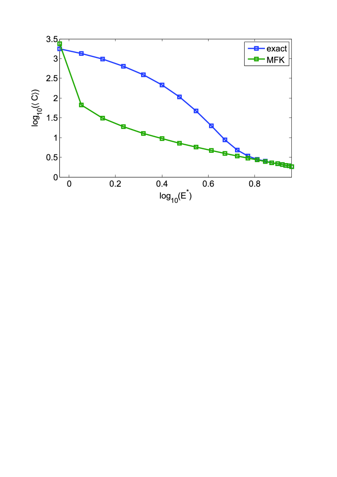
Figure 9: Steady-state substrate mean as a function of the average number of active enzymes. The figure was obtained with the same parametrization used in Fig. 2 of the main paper. It can be clearly seen that in the region where stochastic focusing is observed, the MFK mean grossly underestimates the the true mean of the substrate. However, as the average number of active enzymes increases, MFK becomes increasingly exact.

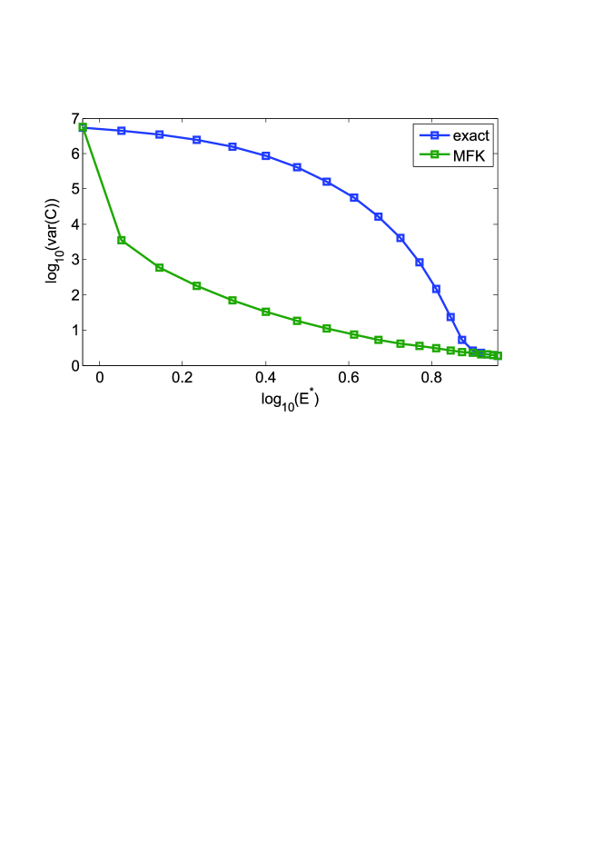
Figure 10: Steady-state substrate variance as a function of the average number of active enzymes. The figure was obtained with the same parametrization used in Fig. 2 of the main paper. We observe that, besides underestimating the mean, MFK also underestimates the the true variance of the substrate. Again, as the average number of active enzymes increases, MFK becomes increasingly exact.

Appendix E Exploring the effect of feedback parameters on substrate and product statistics

Here we present simulation results that explore how the behavior of the SFE network statistics changes under negative feedback. More specifically, we study the effect of feedback on the mean, variance CV and Fano Factor of substrate and product. This analysis helps to put in context our specific choice of feedback parameters used in the main text.

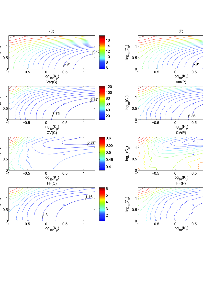
Figure 11: Changes in $C$ and $P$ statistics generated by a scan over feedback parameters ($K_{p}$ and $C_{0}$) under feedback from $C$. As the strength of negative feedback increases (i.e. $K_{p}$ and $C_{0}$ grow), both the mean and variance drop. However, the CV and Fano Factor behave differently: CV appears more sensitive to $C_{0}$ than $K_{p}$, while the Fano Factor depends equally on both parameters. Moreover, the two noise measures become minimal over different regions of the parameter space. As expected, the behavior of substrate fluctuations as parameters vary, is reflected in product fluctuations as well. The feedback parameter set used in the greatest part of the paper ($K_{p}=3$, $C_{0}=5$) is denoted by an asterisk.

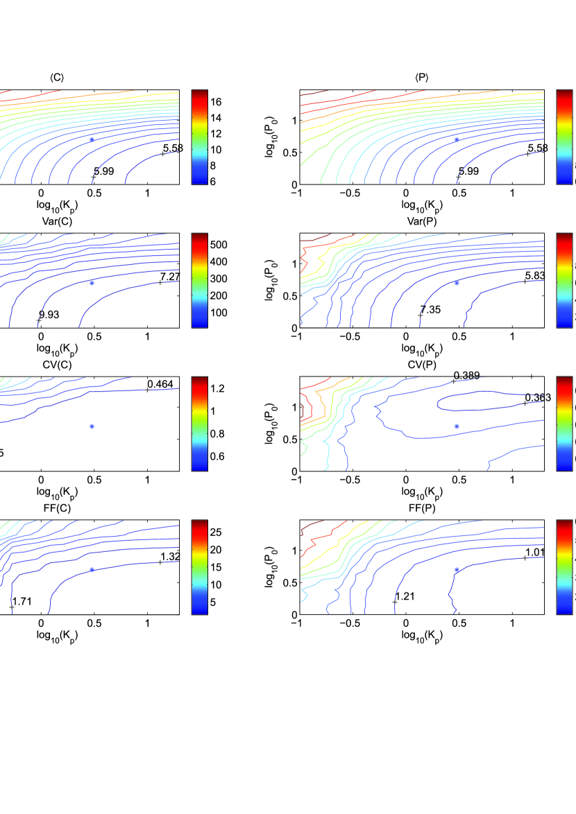
Figure 12: Changes in $C$ and $P$ statistics generated by a scan over feedback parameters ($K_{p}$ and $C_{0}$) under feedback from $P$. It is interesting to note that while the behavior of the $C$ and $P$ means is almost identical to the case of substrate feedback shown above, the noise in $C$ (both in terms of CV and Fano Factor) is significantly increased in the present case. On the other hand, noise in $P$ does not seem decreased in comparison to the case of substrate feedback. In other words, and contrary to the substrate feedback scenario, the behavior of substrate fluctuations is not reflected in product fluctuations. This is perhaps due to a frequency shift in substrate fluctuations, that can no longer be transmitted to $P$ (note that $P$ acts as low-pass filter for upstream fluctuations). The feedback parameter set used in the greatest part of the paper ($K_{p}=3$, $C_{0}=5$) is denoted by an asterisk.

Appendix F Optimization over the feedback parameters using moment closure

Due to the presence of different time scales in the substrate and enzyme dynamics, achieving good accuracy in the calculation of $h$ is hard and thus solving the optimization problem of Section 3.3 for obtaining the best feedback parametrization is a computationally intensive problem. In order to get some idea of the optimal solution in a computationally more tractable setting, we turned to the simple moment closure method devised in [1]. This method, however, requires increasing order derivatives of the reaction rates in general, and of the feedback term in particular.

For this purpose it is therefore preferable to work with a smooth approximation of the feedback term in the form of a Hill function,

$$f(x) =\frac{kx^{n}}{x^{n}+a^{n}}.$$ (25)

Results in the Hill parameter space $(k,n,a)$ can then be transferred back into the piecewise linear form $(K,x_{0})$ of the main manuscript through e.g. a nonlinear least-squares procedure.

The parameter $k$ determines the asymptote of $f$ as $x\to\infty$ and therefore only weakly affects the dynamics in a properly regulated system where large values of $x$ are avoided. To simplify the original problem, we therefore determined a suitable fixed value of $k$ and considered the reduced problem

$$\underset{n,a}{\min}~{}~{}\tilde{h}(n,a):=\langle(C-C_{target})^{2}\rangle=(\langle C\rangle_{ss}-C_{target})^{2}+\mbox{Var}(C)_{ss},$$ (26)

where all moments are now computed from the closed moment equations. The function defined (26) was optimized very efficiently using the derivative-free Nelder-Mead simplex algorithm [4], and also evaluated on a grid in the feedback parameter space, as shown on Fig. 13. The optimal values $n=4.15$ and $a=29.5$ were obtained for $k$ fixed at 160. It can be seen that the objective function varies very little along the red curve; however, intermediate values of $n$ and $a$ seem to be slightly better according to the moment system.

The contours of the same objective function (26), computed with respect to the original stochastic dynamics, is shown on Fig. 14. As the overlay of the red curve from Fig. 13 indicates, this feature is not an artifact of moment closure, but is rather visible in the SSA-based evaluation of the function. The greatest difference from the moment closure result, is that the function now seems to get slightly smaller as $n$ increases. In this respect, the moment closure result can serve as a good initial approximation of the optimal Hill function parameters.

The SSA result reproduces our observation made in Fig. 11 of the main text, as the optimal Hill parametrization results in a step-like function, with very high $n$. For the range of values tested here, the optimal $n$ was found to be around 23 (the upper limit of the search interval), while $a$ was around 18.5. These results agree very well with the results from Fig. 11, where the optimal gain was found to be equal to 30 (again, the upper limit of the search interval) and $C_{0}$ around 16.6, which is very close to the “knee” of the Hill curve with $n=23$, $a=18.5$ and $k=160$.

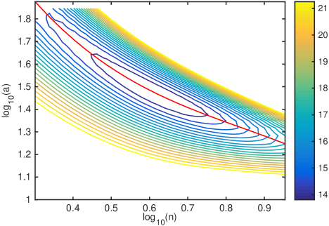
Figure 13: Objective function defined in (26) for the system of moments with a Hill feedback term (assuming feedback from $C$) and moment closure using moments up to order 4. The red line traces the points along which $h$ is varies the least.

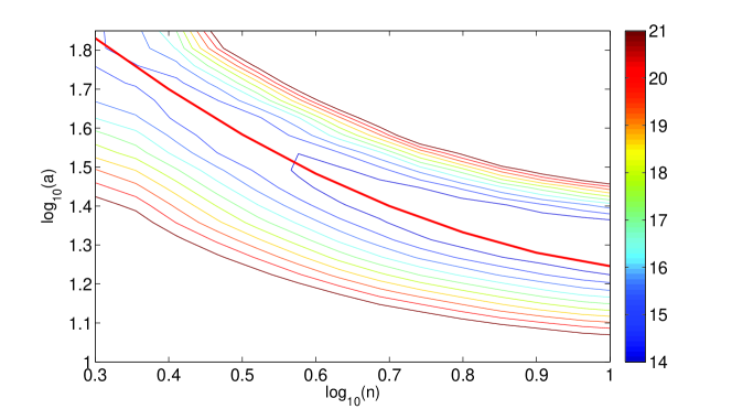
Figure 14: Objective function defined in (26) computed by stochastic simulation, assuming feedback from $C$. The red curve from Fig. 14 is overlaid.

Appendix G How feedback exchanges high gain with robustness

To gain some intuition about the role of high gain in the robustness of feedback system, we consider here a very simple example shown on Fig. 15. The system to be regulated consists of an amplifier A, which is simply model as a gain; that is, when $\beta=0$ and $d=0$, the output $y$ of A is connected to its input $u$ by $y=Au$, where $A$ is the gain of the amplifier. It is also possible that an unwanted signal $d$, the disturbance, corrupts output of A, in which case $y=Au+d$. Assume further that $A$ is very high ($A\gg 1$) but also not known precisely and even fluctuating in time. In this case, a given reference input $r$ will be translated into an output $y$ which inherits the uncertainty in the amplifier gain. Consequently, the output of this so-called open-loop system (obtained for $\beta=0$) can be severely affected by changes in $A$ and disturbance inputs $d$.

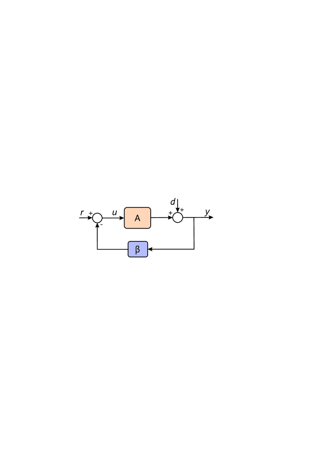
Figure 15: A simple feedback loop.

Let us now consider the closed-loop system, obtained for $\beta>0$. In this case, the output $y$ is multiplied by the feedback gain $\beta$ (which, contrary to $A$, is assumed to be precisely known), subtracted from $r$ and fed back into A. This is typical case of negative feedback because the (scaled) output is subtracted from the input. We can now write the output as

$$y=Ae+d=A(r-\beta y)+d,$$

which implies that

$$y=\frac{A}{1+A\beta}u+\frac{1}{1+A\beta}d.$$

In this case, the closed-loop system gain from $r$ to $y$ has been reduced from $A$ to $A(1+A\beta)^{-1}$. If $A\beta\gg 1$, this ratio is approximately equal to $\beta^{-1}$. In other words, the gain of the closed-loop system is now specified by the feedback gain $\beta$, which is precisely known. The uncertainty in $A$ no longer influences the input-output relation, while the effect of the disturbance is also reduced by a factor of $(1+A\beta)^{-1}$.

References

- [1] Barkai, N., and Leibler, S. Circadian clocks limited by noise. Nature 403 (2000), 267–268. doi:10.1038/35002258.
- [2] Becskei, A., and Serrano, L. Engineering stability in gene networks by autoregulation. Nature 405, 6786 (2000), 590–593.
- [3] Burger, A., Walczak, A. M., and Wolynes, P. G. Influence of decoys on the noise and dynamics of gene expression. Physical Review E 86, 4 (2012), 041920.
- [4] Cross, P. J., Allison, T. M., Dobson, R. C. J., Jameson, G. B., and Parker, E. J. Engineering allosteric control to an unregulated enzyme by transfer of a regulatory domain. Proceedings of the National Academy of Sciences 110, 6 (2013), 2111–2116.
- [5] Deshmukh, M. V., Jones, B. N., Quang-Dang, D.-U., Flinders, J., Floor, S. N., Kim, C., Jemielity, J., Kalek, M., Darzynkiewicz, E., and Gross, J. D. mRNA decapping is promoted by an RNA-binding channel in Dcp2. Molecular cell 29, 3 (2008), 324–336.
- [6] Dorf, R. C., and Bishop, R. H. Modern control systems. Pearson, 2011.
- [7] El-Samad, H., and Khammash, M. Regulated degradation is a mechanism for suppressing stochastic fluctuations in gene regulatory networks. Biophysical journal 90, 10 (2006), 3749–3761.
- [8] El-Samad, H., Kurata, H., Doyle, J., Gross, C., and Khammash, M. Surviving heat shock: control strategies for robustness and performance. Proc. Natl. Acad. Sci. USA 102, 8 (2005), 2736–2741.
- [9] Elf, J., and Ehrenberg, M. Fast evaluation of fluctuations in biochemical networks with the linear noise approximation. Genome research 13, 11 (2003), 2475–2484.
- [10] Engblom, S. Computing the moments of high dimensional solutions of the master equation. Applied Mathematics and Computation 180, 2 (2006), 498 – 515.
- [11] English, B. P., Min, W., van Oijen, A. M., Lee, K. T., Luo, G., Sun, H., Cherayil, B. J., Kou, S., and Xie, X. S. Ever-fluctuating single enzyme molecules: Michaelis-Menten equation revisited. Nature Chemical Biology 2, 2 (2005), 87–94.
- [12] Floor, S. N., Jones, B. N., and Gross, J. D. Control of mRNA decapping by Dcp2: An open and shut case? RNA biology 5, 4 (2008), 189–192.
- [13] Grima, R., Walter, N. G., and Schnell, S. Single-molecule enzymology à la michaelis–menten. FEBS Journal 281, 2 (2014), 518–530.
- [14] Hasenauer, J., Wolf, V., Kazeroonian, A., and Theis, F. Method of conditional moments (MCM) for the chemical master equation. Journal of mathematical biology (2013), 1–49.
- [15] Hornung, G., and Barkai, N. Noise propagation and signaling sensitivity in biological networks: a role for positive feedback. PLoS computational biology 4, 1 (2008), e8.
- [16] Iversen, L., Tu, H.-L., Lin, W.-C., Christensen, S. M., Abel, S. M., Iwig, J., Wu, H.-J., Gureasko, J., Rhodes, C., Petit, R. S., et al. Ras activation by SOS: Allosteric regulation by altered fluctuation dynamics. Science 345, 6192 (2014), 50–54.
- [17] Khammash, M. Robustness in engineering and biology. BMC Biology (submitted).
- [18] Kou, S., Cherayil, B. J., Min, W., English, B. P., and Xie, X. S. Single-molecule Michaelis-Menten equations. The Journal of Physical Chemistry B 109, 41 (2005), 19068–19081.
- [19] Lestas, I., Vinnicombe, G., and Paulsson, J. Fundamental limits on the suppression of molecular fluctuations. Nature 467, 7312 (2010), 174–178. doi:10.1038/nature09333.
- [20] Mashanov, G. I., and Batters, C. Single Molecule Enzymology. Methods in Molecular Biology. Springer, 2011.
- [21] Mazza, C., and Benaim, M. Stochastic Dynamics for Systems Biology. CRC Press, 2014.
- [22] Osella, M., Bosia, C., Corá, D., and Caselle, M. The role of incoherent microrna-mediated feedforward loops in noise buffering. PLoS computational biology 7, 3 (2011), e1001101.
- [23] Paulsson, J., Berg, O. G., and Ehrenberg, M. Stochastic focusing: Fluctuation-enhanced sensitivity of intracellular regulation. Proc. Natl. Acad. Sci. USA 97, 13 (2000), 7148–7153. doi:10.1073/pnas.110057697.
- [24] Raman, S., Taylor, N., Genuth, N., Fields, S., and Church, G. M. Engineering allostery. Trends in Genetics 30, 12 (2014), 521–528.
- [25] Saltelli, A., Ratto, M., Andres, T., Campolongo, F., Cariboni, J., Gatelli, D., Saisana, M., and Tarantola, S. Global sensitivity analysis: the primer. John Wiley & Sons, 2008.
- [26] Samoilov, M., Plyasunov, S., and Arkin, A. P. Stochastic amplification and signaling in enzymatic futile cycles through noise-induced bistability with oscillations. Proc. Natl. Acad. Sci. USA 102, 7 (2005), 2310–2315.
- [27] Sauer, M., Hofkens, J., and Enderlein, J. Handbook of Fluorescence Spectroscopy and Imaging: From Ensemble to Single Molecules. John Wiley & Sons, 2010.
- [28] Sauro, H. M. Enzyme kinetics for systems biology. Ambrosius Publishing, 2012.
- [29] Schwabe, A., Maarleveld, T. R., and Bruggeman, F. J. Exploration of the spontaneous fluctuating activity of single enzyme molecules. FEBS letters 587, 17 (2013), 2744–2752.
- [30] Singh, A., and Hespanha, J. P. Approximate moment dynamics for chemically reacting systems. Automatic Control, IEEE Transactions on 56, 2 (2011), 414–418.
- [31] Swain, P. S. Efficient attenuation of stochasticity in gene expression through post-transcriptional control. Journal of molecular biology 344, 4 (2004), 965–976.
- [32] Thattai, M., and van Oudenaarden, A. Attenuation of noise in ultrasensitive signaling cascades. Biophysical Journal 82, 6 (2002), 2943–2950.
- [33] Togashi, Y., and Kaneko, K. Molecular discreteness in reaction-diffusion systems yields steady states not seen in the continuum limit. Phys. Rev. E 70, 2 (2004), 020901–1. doi:10.1103/PhysRevE.70.020901.
- [34] Tsang, J., Zhu, J., and van Oudenaarden, A. MicroRNA-mediated feedback and feedforward loops are recurrent network motifs in mammals. Molecular Cell 26, 5 (2007), 753–767.
- [35] Ullah, M., and Wolkenhauer, O. Stochastic approaches for systems biology. Springer, 2011.
- [36] Van Kampen, N. Stochastic Processes in Physics and Chemistry (Third Edition). Elsevier, 2007.

References

- [1] Engblom, S. Computing the moments of high dimensional solutions of the master equation. Appl. Math. Comput. 180, 2 (2006), 498–515.
- [2] Gómez-Uribe, C. A., and Verghese, G. C. Mass fluctuation kinetics: Capturing stochastic effects in systems of chemical reactions through coupled mean-variance computations. The Journal of Chemical Physics 126, 2 (2007).
- [3] Hasenauer, J., Wolf, V., Kazeroonian, A., and Theis, F. Method of conditional moments (MCM) for the chemical master equation. Journal of mathematical biology (2013), 1–49.
- [4] Nelder, J. A., and Mead, R. A simplex method for function minimization. The Computer Journal 7, 4 (1965), 308–313.