A new generalization of the Takagi function

Abstract.

We consider a one-parameter family of functions $\{F(t,x)\}_{t}$ on $[0,1]$ and partial derivatives $\partial_{t}^{k}F(t,x)$ with respect to the parameter $t$. Each function of the class is defined by a certain pair of two square matrices of order two. The class includes the Lebesgue singular functions and other singular functions. Our approach to the Takagi function is similar to Hata and Yamaguti. The class of partial derivatives $\partial_{t}^{k}F(t,x)$ includes the original Takagi function and some generalizations. We consider real-analytic properties of $\partial_{t}^{k}F(t,x)$ as a function of $x$, specifically, differentiability, the Hausdorff dimension of the graph, the asymptotic around dyadic rationals, variation, a question of local monotonicity and a modulus of continuity. Our results are extensions of some results for the original Takagi function and some generalizations.

1. Introduction

The Takagi function [14], which is denoted by $T$ throughout the paper, is an example of continuous nowhere differentiable functions and has been considered from various points of view. Since $T$ is a fractal function, it is interesting to investigate real-analytic properties of $T$. For example, differentiability, the Hausdorff dimension of the graph, the asymptotic around dyadic rationals and a modulus of continuity of $T$ have been considered.

Hata and Yamaguti [6] showed the following relation between the Takagi function $T(x)$ and the Lebesgue singular function $L_{a}(x)$ with singularity parameter $a$ :

$$\frac{\partial}{\partial a}\bigg{|}_{a=1/2}L_{a}(x)=T(x).$$ (1.1)

Now give a precise definition of $L_{a}$. Let $\mu_{a}$ be the probability measure on $\{0,1\}$ with $\mu_{a}(\{0\})=a$ and $\mu_{a}^{\otimes\mathbb{N}}$ be the product measure of $\mu_{a}$ on $\{0,1\}^{\mathbb{N}}$. Let $\varphi:\{0,1\}^{\mathbb{N}}\to[0,1]$ be a function defined by $\varphi((x_{n})_{n})=\sum_{n=1}^{\infty}x_{n}/2^{n}$. Let $L_{a}$ be the distribution function of the image measure of $\mu_{a}^{\otimes\mathbb{N}}$ by $\varphi$. $L_{a}$ is identical with $\Phi_{2,1/a}$ in Paradis, Viader and Bibiloni [11].

Recently, de Amo, Díaz Carrillo and Fernández-Sánchez [3] considered $\partial_{a}^{n}L_{a}(x)$ at $a\neq 1/2$. (Here and henceforth $\partial_{z}^{n}$ denotes the $n$-th partial derivatives with respect to the variable $z$. If $n=1$ write simply $\partial_{z}$.) They showed for any $a\neq 1/2$ and for $n\geq 1$, $\partial_{a}^{n}L_{a}(x)$ has zero derivative at almost every $x$. They claimed if $n$ is odd, $\partial_{a}^{n}L_{a}$ is of monotonic type on no open interval (MTNI). That is, on any open interval $J$ in $[0,1]$,

$$-\infty=\inf_{x,y\in J,x\neq y}\frac{\partial_{a}^{n}L_{a}(x)-\partial_{a}^{n}L_{a}(y)}{x-y}<\sup_{x,y\in J,x\neq y}\frac{\partial_{a}^{n}L_{a}(x)-\partial_{a}^{n}L_{a}(y)}{x-y}=+\infty.$$

In this paper we consider a further generalization of $T$ by replacing $L_{a}$ in (1.1) with more general functions and parametrizations. The author’s paper [10] considers a probability measure $\mu_{A_{0},A_{1}}$ on $[0,1]$ defined by a certain pair of two $2\times 2$ real matrices $(A_{0},A_{1})$. $\mu_{A_{0},A_{1}}$ is singular or absolutely continuous with respect to the Lebesgue measure. The class of probability measures in [10] contains not only the Bernoulli measures but also many non-product measures. Parametrize $(A_{0},A_{1})$ by a parameter $t$ around $0$. Assume each component of $A_{0}(t)$ and $A_{1}(t)$ is smooth with respect to $t$ and $(A_{0}(0),A_{1}(0))=(A_{0},A_{1})$. Denote the distribution function of $\mu_{t}$ by $F(t,\cdot)$. That is, $F(t,x)=\mu_{A_{0}(t),A_{1}(t)}([0,x]),x\in[0,1]$.

The main subject of this paper is investigating real analytic properties for the $k$-th partial derivative $f_{k}(x):=\partial^{k}_{t}F(0,x)$. Our framework gives a generalization of $T$. $F(t,x)=L_{a+t}(x)$ for a specific choice of $(A_{0}(t),A_{1}(t))$. Thus our framework contains the one of [3]. Our generalization is different from the ones by [6] and Kôno [7]. The graphs of these curves can be quite different, from Takagi’s classical, $T$, to very asymmetrical ones as shown in figures 1 and 2 below. In Section 2 we will give the framework and show $f_{k}$ is well-defined and continuous on $[0,1]$ for each $k\geq 1$.

In Section 3 we will show the Hausdorff dimension of the graph of $f_{k}$ is $1$. This extends Allaart and Kawamura [1, Corollary 4.2] and is applicable to the framework in [3, Section 5]. Our proof is different from Mauldin and Williams [9] and [1] and seems simpler than them because we do not need to investigate strength of continuity of $f_{k}$. In Section 4 we will show the derivative of $f_{k}$ is $0$ almost everywhere. This extends [3, Theorems 12 and 13]. We will examine the asymptotic of $f_{k}$ around dyadic rationals in Section 5. The asymptotic of $f_{k}$ around dyadic rationals and around Lebesgue-a.e. points can be similar on the one hand but can be considerably different on the other hand. As shown in Figure 1 there is a fractal function whose derivatives are zero at all dyadic rationals. To our knowledge such a fractal function is unusual.

If we consider the case $k=1$ and the “linear” case, each of which contains the original Takagi function $T$, we have more sophisticated results. In Theorem 6.2 we will consider differentiability and variation of $f_{k}$. [3, Theorem 14] states if we consider the “linear” case and $k$ is odd, $f_{k}$ is MTNI. Theorem 6.3 will extend [3, Theorem 14] to all $k\geq 1$. If $\mu_{0}$ is singular, the asymptotic of $f_{k}$ around $\mu_{0}$-a.s. points and around Lebesgue-a.e. points can be considerably different. In Section 7 we will consider a modulus of continuity of $f_{1}$. Theorem 7.3 will extend Allaart and Kawamura [2, Theorem 5.4], which gives a necessary and sufficient condition for the existence of

$$\lim_{h\to 0}\frac{T(x+h)-T(x)}{h\log_{2}(1/|h|)}\ \ \text{ at non-dyadic $x$. }$$

Theorem 7.7 will investigate a modulus of continuity of $f_{1}$ at $\mu_{0}$-a.s. points. It is similar to [7]. We have the original Takagi function case of [7] by our approach. Our proofs are different from [2] and [7]. We do not use [7, Lemma 3] which plays an important role in [2] and [7].

2. Framework

2.1. Definition of $\mu_{A_{0},A_{1}}$

Let $A_{i}=\begin{pmatrix}a_{i}&b_{i}\\ c_{i}&d_{i}\end{pmatrix}$, $i=0,1$, be two real $2\times 2$ matrices such that the following hold :
(i) $0=b_{0}<\dfrac{a_{0}+b_{0}}{c_{0}+d_{0}}=\dfrac{b_{1}}{d_{1}}<\dfrac{a_{1}+b_{1}}{c_{1}+d_{1}}=1$.
(ii) $a_{i}d_{i}-b_{i}d_{i}>0$, $i=0,1$.
(iii) $(a_{i}d_{i}-b_{i}d_{i})^{1/2}<\min\{c_{i},c_{i}+d_{i}\}$, $i=0,1$.

Consider a functional equation for $f:[0,1]\to\mathbb{R}$ :

$$f(x)=\begin{cases}\Phi\left(A_{0},f(2x)\right)&0\leq x\leq 1/2\\ \Phi\left(A_{1},f(2x-1)\right)&1/2\leq x\leq 1,\end{cases}\ \ \text{where }\Phi(A,z):=\dfrac{az+b}{cz+d}\text{ for }A=\begin{pmatrix}a&b\\ c&d\end{pmatrix}.$$ (2.1)

Conditions (i) - (iii) assure the existence of a unique continuous solution for (2.1). (2.1) is a special case of de Rham’s functional equations [12]. Let $\mu_{A_{0},A_{1}}$ be the measure such that the unique continuous solution $f$ of (2.1) is the distribution function of $\mu_{A_{0},A_{1}}$. By conditions (i) - (iii) we can represent all components of $A_{0},A_{1}$ by $b_{1},c_{0}$ and $c_{1}$. We can assume $d_{0}=d_{1}=1$. Conditions (i) - (iii) imply $a_{0}=b_{1}(c_{0}+1)$, $b_{0}=0$, $a_{1}=1-b_{1}+c_{1}$ and

$$b_{1}\in(0,1),c_{0}\in\left(b_{1}-1,\frac{1}{b_{1}}-1\right),c_{1}\in\left(-b_{1},\frac{b_{1}}{1-b_{1}}\right).$$ (2.2)

If $b_{1}=a$ and $c_{0}=c_{1}=0$ the Lebesgue singular function $L_{a}$ is the distribution function of $\mu_{A_{0},A_{1}}$. $c_{0}=c_{1}=0$ if and only if both $\Phi(A_{0};\cdot)$ and $\Phi(A_{1};\cdot)$ are linear functions. By [10, Theorem 1.2], $\mu_{A_{0},A_{1}}$ is absolutely continuous if $c_{0}=(2b_{1})^{-1}-1$ and $c_{1}=1-2b_{1}$, and singular otherwise. Let

$$\alpha:=\min\left\{0,\frac{c_{0}}{1-b_{1}(c_{0}+1)},\frac{c_{1}}{b_{1}}\right\}\text{ and }\beta:=\max\left\{0,\frac{c_{0}}{1-b_{1}(c_{0}+1)},\frac{c_{1}}{b_{1}}\right\}.$$

$\alpha=\beta=0$ if and only if $c_{0}=c_{1}=0$. Roughly speaking $\alpha$ and $\beta$ measure how $\mu_{A_{0},A_{1}}$ is “far” from the Bernoulli measures.

Now define a “dual” $(\widetilde{A}_{0},\widetilde{A}_{1})$ associated with $(A_{0},A_{1})$ in order to shorten some proofs.

Definition 2.1 (Dual matrices).

Let

$$(\widetilde{b}_{1},\widetilde{c}_{0},\widetilde{c}_{1}):=\left(1-b_{1},-\frac{c_{1}}{1+c_{1}},-\frac{c_{0}}{1+c_{0}}\right),$$ (2.3)

Define $\widetilde{A}_{i},i=0,1$, $\widetilde{\alpha}$ and $\widetilde{\beta}$ by substituting $(\widetilde{b}_{1},\widetilde{c}_{0},\widetilde{c}_{1})$ for $(b_{1},c_{0},c_{1})$ in the definition of $A_{i}$, $\alpha$ and $\beta$. (2.2) holds for $(\widetilde{A}_{0},\widetilde{A}_{1})$ if and only if it holds for $(A_{0},A_{1})$. We have

$$\mu_{\widetilde{A}_{0},\widetilde{A}_{1}}([0,x])=\mu_{A_{0},A_{1}}([1-x,1]),\,x\in[0,1].$$ (2.4)

$$\widetilde{\widetilde{A_{i}}}=A_{i},\,i=0,1.$$ (2.5)

2.2. Parametrization

(1) In addition to (2.2) we assume either the Lipschitz constant of $\Phi\left({}^{t}\!A_{1};y\right)$ on $y\in[\alpha,\beta]$ or the Lipschitz constant of $\Phi\left({}^{t}\!\widetilde{A}_{1};y\right)$ on $y\in\left[\widetilde{\alpha},\widetilde{\beta}\right]$ is strictly less than $1$. That is

$$(1+c_{1})\left(1-b_{1}(1+c_{0})\right)^{2}<1-b_{1}\text{ or }(b_{1}+c_{1})^{2}<b_{1}(1+c_{0})(1+c_{1}).$$ (2.6)

Assume this condition by a difficulty arising in computation in Lemma 2.5 below. However if $c_{0}=c_{1}=0$, (2.6) holds. The Lipschitz constant of $\Phi\left({}^{t}\!A_{0};y\right)$ on $y\in[\alpha,\beta]$ and the Lipschitz constant of $\Phi\left({}^{t}\!\widetilde{A}_{0};y\right)$ on $y\in\left[\widetilde{\alpha},\widetilde{\beta}\right]$ are strictly less than $1$.

(2) Conditions (2.2) and (2.6) define an open set $E$ in $\mathbb{R}^{3}$ in which we will consider different curves.

$$E:= \left\{(x,y,z)\in\mathbb{R}^{3}\ \bigg{|}\ 0<x<1,x-1<y<\frac{1-x}{x},-x<z<\frac{x}{1-x}\right\}$$

$$\ \ \cap\bigl{\{}(x,y,z)\big{|}(1+z)(1-x(1+y))^{2}<1-x\text{ or }(x+z)^{2}<x(1+y)(1+z)\bigr{\}}.$$

(3) Fix a point $(b_{0},c_{0},c_{1})\in E$. We consider a smooth curve $(b_{1}(t),c_{0}(t),c_{1}(t))$ in $E$ on an open interval containing $0$ such that $(b_{1}(0),c_{0}(0),c_{1}(0))=(b_{0},c_{0},c_{1})$.

Define $A_{0}(t),A_{1}(t),\alpha(t),\beta(t)$ by substituting $(b_{1}(t),c_{0}(t),c_{1}(t))$ for $(b_{1},c_{0},c_{1})$ in the definition of $A_{0},A_{1},\alpha,\beta$. Let

$$\mu_{t}:=\mu_{A_{0}(t),A_{1}(t)}\text{ and }F(t,x):=\mu_{t}([0,x]),\ \ x\in[0,1].$$

This class of smooth curves includes the frameworks of [1], [2], [3] and [6]. We have

$$\{(x,0,0):0<x<1\}\subset E.$$

If $(b_{1}(t),c_{0}(t),c_{1}(t))=(t+a,0,0)$, $F(0,x)=L_{a}(x)$.

2.3. Notation and lemma

Let $X_{i}(x):=z_{i}$ if $x=\sum_{n\geq 1}2^{-n}z_{n}$ is the dyadic expansion of $x$.

Definition 2.2.

(i)

$$G_{j}(t,y):=\Phi\left({}^{t}\!A_{j}(t);y\right),\ y\in[\alpha(t),\beta(t)],j=0,1.$$ (2.7)

(ii)

$$p_{0}(t,y):=\frac{y+1}{y+b_{1}(t)^{-1}}\text{ and }p_{1}(t,y):=1-p_{0}(t,y),\ y\in[\alpha(t),\beta(t)].$$

(iii) Let $p_{min}(t)$ and $p_{\text{max}}(t)$ be the minimum and maximum of $\left\{p_{0}(t,\alpha(t)),p_{1}(t,\beta(t))\right\}$.
(iv)

$$g_{0}(t,x):=0\text{ and }g_{i}(t,x):=G_{X_{i}(x)}\left(t,g_{i-1}(t,x)\right),\ \ x\in[0,1),i\geq 1.$$

(v)

$$H_{n}(t,x):=p_{X_{n+1}(x)}\left(t,g_{i}(t,x)\right),\ \ P_{n}(t,x):=p_{0}\left(t,g_{n}(t,x)\right),\ \ x\in[0,1).$$

(vi)

$$M_{n}(t,x):=\prod_{i=0}^{n-1}H_{i}(t,x),\ \ x\in[0,1).$$

Example 2.3.

If $c_{0}(t)=c_{1}(t)=0$ then for $x\in[0,1)$

$$G_{0}(t,x)=b_{1}(t)x,\ \ G_{1}(t,x)=(1-b_{1}(t))x.$$

$$\alpha(t)=g_{n}(t,x)=\beta(t)=0,\ \ n\geq 0.$$

$$p_{0}(t,0)=P_{n}(t,x)=b_{1}(t)=1-p_{1}(t,0),\ \ n\geq 0.$$

$$p_{min}(t)=\min\{b_{1}(t),1-b_{1}(t)\}\text{ and }p_{max}(t)=\max\{b_{1}(t),1-b_{1}(t)\}.$$

$$H_{n}(t,x)=b_{1}(t)1_{\{X_{n+1}(x)=0\}}(x)+(1-b_{1}(t))1_{\{X_{n+1}(x)=1\}}(x).$$

$$M_{n}(t,x)=b_{1}(t)^{a_{n,0}}(1-b_{1}(t))^{n-a_{n,0}}\text{ where }a_{n,0}:=\left|\{1\leq i\leq n:X_{i}(x)=0\}\right|.$$

In this case we do not need to introduce $G,g,p,P,H\text{ and }M$. However we would like to consider the case that $c_{0}(t)=c_{1}(t)=0$ fails. $G_{i},g_{n},p_{i},H_{n}\text{ and }M_{n}$ are defined in order to give a useful expression for $F(t,x)$ in (2.11) below.

The following are easy to see so the details are left to readers.

Lemma 2.4.

For $n\geq 0$ and $x\in[0,1)$
(i)

$$\alpha(t)\leq g_{n}(t,x)\leq\beta(t),\ \$$ (2.8)

(ii)

$$0<p_{\text{min}}(t)\leq H_{n}(t,x)\leq p_{\text{max}}(t)<1.$$ (2.9)

(iii)

$$\mu_{t}\left([x_{n},x_{n}+2^{-n})\right)=M_{n}(t,x).$$ (2.10)

(iv)

$$F(t,x)=\sum_{n=0}^{+\infty}X_{n+1}(x)\left(M_{n}(t,x)-M_{n+1}(t,x)\right).$$ (2.11)

By (i) $g_{n}(t,x),H_{n}(t,x),P_{n}(t,x)$ and $M_{n}(t,x)$ are well-defined for any $n$ and $x$.

Define $(\widetilde{b}_{1}(t),\widetilde{c}_{0}(t),\widetilde{c}_{1}(t))$ and $(\widetilde{A}_{0}(t),\widetilde{A}_{1}(t))$ by substituting $(b_{1}(t),c_{0}(t),c_{1}(t))$ in Definition 2.1. By (2.5) $(\widetilde{b}_{1}(t),\widetilde{c}_{0}(t),\widetilde{c}_{1}(t))$ is also a smooth curve in $E$. Define $\widetilde{\mu}_{t},\widetilde{F},\widetilde{G}_{j},\widetilde{g}_{n},\widetilde{p}_{j},\widetilde{P}_{i},\widetilde{H}_{i},\widetilde{M}_{n},\widetilde{p}_{\text{min}}$ and $\widetilde{p}_{\text{max}}$ in the same manner by substituting $(\widetilde{b}_{0},\widetilde{c}_{0},\widetilde{c}_{1})$ for $(b_{0},c_{0},c_{1})$. Lemma 2.4 hold also for $\widetilde{g}_{i},\widetilde{H}_{n},\widetilde{M}_{n},\widetilde{\mu}_{t},\widetilde{p}_{\text{min}}$ and $\widetilde{p}_{\text{max}}$.

2.4. Well-definedness and continuity of $f_{k}$

(2.6) has been introduced in order to establish a uniform boundedness for $\partial_{t}^{k}H_{n}(t,x)$ as follows.

Lemma 2.5.

For any $k\geq 0$ there is a continuous function $C_{1,k}(t)$ on a neighborhood of $t=0$ such that for each $t$ in the neighborhood :

$$\sup_{n\geq 0,x\in(0,1)}\left|\partial_{t}^{k}H_{n}(t,x)\right|\leq C_{1,k}(t)$$

Proof.

The case $k=0$ follows from (2.9). Assume $k\geq 1$. Then $\left|\partial_{t}^{k}H_{n}(t,x)\right|=\left|\partial_{t}^{k}P_{n}(t,x)\right|$.

Recall (2.6). Assume $(1+c_{1})\left(1-b_{1}(1+c_{0})\right)<1-b_{1}$. Then

$$(1+c_{1}(t))\left(1-b_{1}(t)(1+c_{0}(t))\right)<1-b_{1}(t)$$ (2.12)

holds if $t$ is close to $0$.

Since $\partial_{t}^{k}P_{n}(t,x)$ is a multivariate polynomial consisting of

$$\partial_{t}^{j}g_{n}(t,x) \partial_{t}^{j^{\prime}}\partial_{y}^{j^{\prime\prime}}P_{n}(t,x) 0\leq j,j^{\prime},j^{\prime\prime}\leq i$$ and ,

as variables, it suffices to show that for each $k\geq 1$ there is a continuous function $C_{2,k}(t)$ such that

$$\sup_{n\geq 0,x\in(0,1)}\left|\partial_{t}^{k}g_{n}(t,x)\right|\leq C_{2,k}(t)<+\infty.$$ (2.13)

We now show (2.13) by induction on $k$. The case $k=0$ follows from (2.8). Assume (2.13) holds for $k=0,1,\dots i-1$. Then

$$\partial_{t}^{i}g_{n}(t,x)=\partial_{y}G_{X_{n}(x)}(t,g_{n-1}(t,x))\partial_{t}^{i}g_{n-1}(t,x)+\text{Poly}(i,n).$$

Here $\text{Poly}(i,n)$ is a multivariate polynomial consisting of

$$\partial_{t}^{j}g_{n-1}(t,x) \partial_{t}^{j^{\prime}}\partial_{y}^{j^{\prime\prime}}G_{X_{n}(x)}(t,g_{n-1}(t,x)) 0\leq j,j^{\prime},j^{\prime\prime}\leq i-1$$ and ,

as variables.

By the hypothesis of induction and (2.8), for each $i$, there is a continuous function $C_{3,i}(t)$ such that

$$\left|\partial_{t}^{i}g_{n}(t,x)\right|\leq\left(\max_{l\in\{0,1\},y\in[\alpha(t),\beta(t)]}\partial_{y}G_{l}(t,y)\right)\left|\partial_{t}^{i}g_{n-1}(t,x)\right|+C_{3,i}(t).$$

By (2.12)

$$\max_{l\in\{0,1\},y\in[\alpha(t),\beta(t)]}\partial_{y}G_{l}(t,y)<1.$$

Therefore

$$\sup_{n\geq 0,x\in(0,1)}\left|\partial_{t}^{i}g_{n}(t,x)\right|\leq\frac{C_{3,i}(t)}{1-\max_{l\in\{0,1\},y\in[\alpha(t),\beta(t)]}\partial_{y}G_{l}(t,y)}.$$

Hence (2.13) holds.

Second assume $(b_{1}+c_{1})^{2}<b_{1}(1+c_{0})(1+c_{1})$. By (2.3) and continuity of $(b_{1}(t),c_{0}(t),c_{1}(t))$

$$(1+\widetilde{c}_{1}(t))\left(1-\widetilde{b}_{1}(t)(1+\widetilde{c}_{0}(t))\right)<1-\widetilde{b}_{1}(t)$$

holds if $t$ is close to $0$. The rest of the proof goes in the same manner as above. ∎

Let

$$x_{n}:=\sum_{i=1}^{n}\frac{X_{i}(x)}{2^{i}},\ \ x\in[0,1)\ \text{ and }\ D:=\bigcup_{n\geq 1}\left\{\frac{k}{2^{n}}\ \bigg{|}\ 1\leq k\leq 2^{n}-1\right\}.$$

Theorem 2.6.

(i) For any $k\geq 0$ there is $C_{k}>0$ such that

$$\left|\frac{\partial_{t}^{k}F(0,x_{n}+2^{-n})-\partial_{t}^{k}F(0,x_{n})}{F(0,x_{n}+2^{-n})-F(0,x_{n})}\right|\leq C_{k}n^{k},\,x\in[0,1),n\geq 1.$$ (2.14)

(ii) $\partial_{t}^{k}F(0,x)$ is well-defined for any $x\in[0,1]\setminus D$.
(iii) Let $C_{k}$ be the constant above. Then

$$\left|\frac{\partial_{t}^{k}F(0,x)-\partial_{t}^{k}F(0,y)}{F(0,x)-F(0,y)}\right|\leq C_{k}(-\log_{2}|x-y|)^{k},\,x\neq y.$$ (2.15)

Now we can define

$$f_{k}(x):=\partial_{t}^{k}F(0,x)\text{ and }\Delta_{k}F(x,y):=\frac{\partial_{t}^{k}F(0,x)-\partial_{t}^{k}F(0,y)}{F(0,x)-F(0,y)},\,\,x\neq y,\,k\geq 0.$$

By (2.15), $f_{k}$ is continuous and if $\mu_{0}$ is absolutely continuous

$$\left|f_{k}(x)-f_{k}(y)\right|=O\left(|x-y|\left(-\log_{2}|x-y|\right)^{k}\right).$$ (2.16)

Whether (2.15) is best or not will be discussed after Theorem 5.4. The key of the proof of (i) is giving an upper bound for $\left|\partial_{t}^{l}H_{j}(t,x)\right|$ uniform with respect to $x$ by Lemma 2.5. For (ii), roughly speaking, the key is showing the exchangeability of the differential $\partial_{t}$ with the infinite sum in (2.11), by using (2.9). (iii) follows from (i) and (ii) easily.

Proof.

By (2.10)

$$\frac{\partial_{t}^{k}F(t,x_{n}+2^{-n})-\partial_{t}^{k}F(t,x_{n})}{F(t,x_{n}+2^{-n})-F(t,x_{n})}=\frac{\partial_{t}^{k}M_{n}(t,x)}{M_{n}(t,x)}.$$

There exist positive integers $\left\{r(k,(k_{j})_{j}):\sum_{j}k_{j}=k,k_{j}\geq 0\right\}$ such that

$$\sum_{k_{j}\geq 0,\sum_{j=0}^{n-1}k_{j}=k}r(k,(k_{j})_{j})=n^{k}\ \ \ \text{ and }$$ (2.17)

$$\partial_{t}^{k}M_{n}(t,x)=\sum_{k_{j}\geq 0,\,\sum_{j=0}^{n-1}k_{j}=k}C(k,(k_{j})_{j})\left(\prod_{j=0}^{n-1}\partial_{t}^{k_{j}}H_{j}(t,x)\right).$$

We now compare $\partial_{t}^{k_{j}}H_{j}(t,x)$ with $H_{j}(t,x)$. Since the number of $j$ such that $k_{j}>0$ is less than or equal to $k$,

$$\left|\prod_{j=0}^{n-1}\frac{\partial_{t}^{k_{j}}H_{j}(t,x)}{H_{j}(t,x)}\right|=\left|\prod_{j:0<k_{j}\leq k}\frac{\partial_{t}^{k_{j}}H_{j}(t,x)}{H_{j}(t,x)}\right|\leq\left(\frac{\max_{0\leq l\leq k,j\geq 0,x\in[\alpha(t),\beta(t)]}\left|\partial_{t}^{l}H_{j}(t,x)\right|}{\min_{j\geq 0,x\in[\alpha(t),\beta(t)]}H_{j}(t,x)}\right)^{k}.$$

Lemma 2.5 implies for each $l\geq 0$

$$\max_{j\geq 0,x\in[\alpha(t),\beta(t)]}\left|\partial_{t}^{l}H_{j}(t,x)\right|\leq C_{1,l}(t)<+\infty.$$

By (2.17)

$$\left|\frac{\partial_{t}^{k}M_{n}(t,x)}{M_{n}(t,x)}\right|\leq\sum_{k_{j}\geq 0,\ \sum_{j=0}^{n-1}k_{j}=k}r(k,(k_{j})_{j})C_{4,k}(t)=C_{4,k}(t)n^{k},$$ (2.18)

where $C_{4,k}(t):=\max_{0\leq l\leq k}C_{1,l}(t)$. This is continuous with respect to $t$. Thus we have (i).

By (2.18) and (2.9) there is an open interval $(a,b)$ containing $0$ such that

$$\max_{t\in[a,b]}C_{4,k}(t)<+\infty,\ \ \max_{t\in[a,b]}p_{\text{max}}(t)<1\ \ \text{ and}$$

$$\sum_{n}\max_{t\in[a,b]}\left|\partial^{k}_{t}F(t,x_{n+1})-\partial^{k}_{t}F(t,x_{n})\right|\leq\max_{t\in[a,b]}C_{4,k}(t)\cdot\sum_{n\geq 0}n^{k}\left(\max_{t\in[a,b]}p_{\text{max}}(t)\right)^{n}.$$ (2.19)

Recall (2.11). Thus we have (ii).

(2.19) implies $\left|f_{k}(x)-f_{k}(y)\right|=\lim_{n\to\infty}\left|f_{k}(x_{n})-f_{k}(y_{n})\right|$. This and (2.14) imply (2.15). The continuity of $\partial^{k}_{t}F(0,x)$ with respect to $x$ follows from (2.15) and the continuity of $F(x)$. Thus we have (iii). ∎

Hereafter, if $t=0$ we often omit $t$ and write $F(x)=F(0,x)$ and $\widetilde{F}(x)=\widetilde{F}(0,x)$.

3. Hausdorff dimension

Theorem 3.1.

For any $k\geq 1$, the Hausdorff dimension of the graph of $f_{k}$ is $1$.

This extends [1, Corollary 4.2] and is applicable to the framework in [3, Section 5]. If $f_{1}=T$, this follows from [9]. For proof we will choose a “good” family of coverings of the graph of $f_{k}$ and then show $\dim_{H}\{(x,f_{k}(x)):x\in[0,1]\}\leq s$ for any $s>1$. The key point is using the simple fact that $F$ is the distribution function of $\mu_{0}$. Our proof is different from [9] and [1] and seems simpler than them because we do not need to investigate strength of continuity of $f_{k}$ such as (2.16) and the Hölder exponent. As we will see in Theorem 5.7 (ii) later $f_{k}$ may not be $\eta$-Hölder continuous if $\eta<1$ is sufficiently close to $1$.

Proof.

Hereafter, “$\dim_{H}$” denotes the Hausdorff dimension and “diam” denotes the diameter. It is easy to see $\dim_{H}\{(x,f_{k}(x)):x\in[0,1]\}\geq 1$. We now show $\dim_{H}\{(x,f_{k}(x)):x\in[0,1]\}\leq s$ for any $s>1$. Let

$$O\left(f_{k},n,l\right):=\max_{x\in[(l-1)/2^{n},l/2^{n}]}\left|f_{k}(x)-f_{k}\left(\frac{l-1}{2^{n}}\right)\right|\text{ and }$$

$$R(k;n,l):=\left[\frac{l-1}{2^{n}},\frac{l}{2^{n}}\right]\times\left[f_{k}\left(\frac{l-1}{2^{n}}\right)-O\left(f_{k},n,l\right),\,f_{k}\left(\frac{l-1}{2^{n}}\right)+O\left(f_{k},n,l\right)\right].$$

Then $\cup_{l=1}^{2^{n}}R(k;n,l)$ covers the graph of $f_{k}$ and

$$\text{diam}\left(R(k;n,l)\right)=(4^{-n}+4O\left(f_{k},n,l\right)^{2})^{1/2}.$$

If $s>1$,

$$\left(4^{-n}+4O\left(f_{k},n,l\right)^{2}\right)^{s/2}\leq\left(2^{-n}+2O\left(f_{k},n,l\right)\right)^{s}\leq 2^{s-1}\left(2^{-sn}+2^{s}O\left(f_{k},n,l\right)^{s}\right).$$

Therefore it suffices to show that

$$\lim_{n\to\infty}\sum_{l=1}^{2^{n}}O\left(f_{k},n,l\right)^{s}=0.$$ (3.1)

By (2.15)

$$O\left(f_{k},n,l\right)\leq C_{k}\max_{x\in[(l-1)/2^{n},l/2^{n}]}\left(-\log_{2}\left|x-\frac{l-1}{2^{n}}\right|\right)^{k}\left(F(x)-F\left(\frac{l-1}{2^{n}}\right)\right).$$

Using this and

$$\sum_{l=1}^{2^{n}}F\left(\frac{l}{2^{n}}\right)-F\left(\frac{l-1}{2^{n}}\right)=1,$$

$$\sum_{l=1}^{2^{n}}O\left(f_{k},n,l\right)^{s}\leq C_{k}^{s}\max_{x,y\in[0,1],0<|x-y|\leq 2^{-n}}\left(-\log_{2}|x-y|\right)^{sk}\left|F(x)-F(y)\right|^{s-1}.$$

Let $z<w$ and $n=n_{z,w}$ be the smallest number $n$ such that $z\leq(k-1)/2^{n}<k/2^{n}\leq w$ for some $k$. Then $z\geq\min\{0,(k-3)/2^{n}\}$ and $w\leq\max\{1,(k+2)/2^{n}\}$. By (2.9), $p_{\text{max}}(0)<1$ and $\max_{v\in(0,1)}\mu_{0}([v_{n},v_{n}+2^{-n}))\leq p_{\text{max}}(0)^{n}$. Hence

$$F(y)-F(x)\leq F\left(\max\{1,(k+2)/2^{n}\}\right)-F\left(\min\{0,(k-3)/2^{n}\}\right)\leq 5p_{\text{max}}(0)^{n}.$$

Hence

$$|F(z)-F(w)|\leq 5|z-w|^{c},\,\,z,w\in[0,1],\ \ \text{ for $c=-\log_{2}p_{\text{max}}(0)>0$. }$$

Using this and $s>1$,

$$\lim_{n\to\infty}\max_{x,y\in[0,1],0<|x-y|\leq 2^{-n}}\left(-\log_{2}|x-y|\right)^{sk}\left|F(x)-F(y)\right|^{s-1}=0.$$

Thus we have (3.1). ∎

4. Local Hölder continuity at almost every points

Theorem 4.1.

There is $c\geq 1$ such that for any $k\geq 0$ there is $C_{k}^{\prime}<+\infty$ such that

$$\limsup_{h\to 0}\frac{|f_{k}(x+h)-f_{k}(x)|}{|h|^{c}}\leq C_{k}^{\prime}\,\,\text{ Lebesgue-a.e.$x$.}$$

If $\mu_{0}$ is singular, $c>1$ and $C_{k}^{\prime}=0$ for any $k$. If $\mu_{0}$ is absolutely continuous, $c=1$.

This is more general than [3, Theorems 12 and 13] which investigates the case $(b_{1}(t),c_{0}(t),c_{1}(t))=(t+a,0,0)$, $a\neq 1/2$ only. Our approach is partly similar to the proof of [3, Theorem 12] but seems more general and clearer than it. The key point is showing the following : (1) Giving a nice upper bound for $|F(x)-F(y)|$ in terms of $M_{m}(0,x)$ by (2.11) and (2.9). (2) $M_{m}(0,x)$ decays rapidly by (4.2) below. (3) Giving a nice lower bound for $|x-y|$ by assuming $x$ is a normal number as the proof of [3, Theorem 12].

Let

$$\left\{m_{1}(z)<m_{2}(z)<\cdots\right\}:=\left\{i\geq 1:X_{i}(z)=1\right\},\ \ z\in[0,1).$$ (4.1)

$$n(x,y):=\min\left\{n:m_{k}(x)=m_{k}(y)\text{ for any }k\leq n\right\},\ \ x,y\in(0,1)\setminus D\text{ with }x\neq y.$$

In a manner similar to the proof of [10, Theorem 1.2], there is a constant $c\geq 1$ such that

$$\liminf_{n\to\infty}\frac{-\log_{2}M_{n}(0,x)}{n}\geq c\ \ \text{ Lebesgue-a.e.$x$.}$$ (4.2)

If $\mu_{0}$ is singular, $c>1$. If $\mu_{0}$ is absolutely continuous, $c=1$.

Proof.

This assertion is trivial if $\mu_{0}$ is absolutely continuous. Assume $\mu_{0}$ is singular and $x$ is a normal number. Using (2.15), it suffices to show

$$\lim_{h\to 0}\frac{|F(x+h)-F(x)|}{|h|^{c}}=0\ \ \ \text{ Lebesgue-a.e.$x$ \ for some $c>1$.}$$ (4.3)

Let $y\in(0,1)\setminus(D\cup\{x\})$ and Let $m:=m_{n(x,y)}(x)$. Then $X_{k}(x)=X_{k}(y)$ and $M_{k}(0,x)=M_{k}(0,y)$ for any $k\leq m_{n(x,y)}(x)$. By (2.11) and (2.9),

$$\left|F(x)-F(y)\right|\leq\sum_{i\geq m}\left|M_{i}(0,x)-M_{i}(0,y)\right|\leq CM_{m}(0,x).$$ (4.4)

Here $C$ denotes a constant independent from $x,y$.

We now give a lower bound of $|x-y|$ in terms of $n(x,y)$. If $x>y$, $m_{n(x,y)+1}(x)<m_{n(x,y)+1}(y)$ and hence

$$x-y\geq 2^{-m_{n(x,y)+2}(x)}.$$

If $x<y$, $m_{n(x,y)+1}(x)>m_{n(x,y)+1}(y)$ and hence

$$y-x\geq 2^{-m_{n(x,y)+1}(x)}-\sum_{j\geq n(x,y)+2}2^{-m_{j}(x)}.$$

Since $x$ is normal,

$$|x-y|\geq 2^{-m_{n(x,y)+2}(x)\cdot(1+o(1))},\,y\to x.$$ (4.5)

By (4.2) and $\displaystyle\lim_{k\to+\infty}\dfrac{m_{k+2}(x)}{m_{k}(x)}=1$, there is $c>1$ such that

$$\lim_{k\to\infty}2^{c\cdot m_{k+2}(x)}M_{m_{k}(x)}(0,x)=0$$ (4.6)

holds for Lebesgue-a.e. normal number $x$. We also have $\lim_{y\to x}n(x,y)=+\infty$. Now (4.3) follows from (4.4), (4.5) and (4.6). ∎

5. Asymptotics of $f_{k}$ around dyadic rationals

5.1. Lemmas

Recall the definition of $g_{i}$, $P_{i}$ and $H_{i}$ in Definition 2.2. Then

$$\partial_{t}P_{i}(t,x)=\frac{b_{1}^{\prime}(t)(g_{i}(t,x)+1)+b_{1}(t)(1-b_{1}(t))\partial_{t}g_{i}(t,x)}{\left(b_{1}(t)g_{i}(t,x)+1\right)^{2}}.$$ (5.1)

Let

$$D_{n}:=\left\{\frac{k}{2^{n}}:1\leq k\leq 2^{n}-1\right\},\ \ n\geq 1\ \text{ and }\ D_{0}:=\emptyset.$$

Lemma 5.1.

(i)

$$\lim_{i\to\infty}\sup_{y\in D_{k}\setminus D_{k-1},k\geq 1}\left|H_{i+k}(0,y)-b_{1}(1+c_{0})\right|=0.$$ (5.2)

This also holds if we substitute $\widetilde{H}_{i+k},\widetilde{b}_{1}\text{ and }\widetilde{c}_{0}$ for $H_{i+k},b_{1},\text{ and }c_{0}$.
(ii) If $x\in D$,

$$\lim_{n\to\infty}\frac{\partial_{t}H_{n}(0,x)}{H_{n}(0,x)}=\frac{b_{1}^{\prime}(0)}{b_{1}}+\frac{c_{0}^{\prime}(0)}{1+c_{0}}$$ (5.3)

Convergences (5.2) and (5.3) are exponentially fast.

Proof.

Recall the definition of $G_{i}$ in (2.7). Let $G_{0,i}$ be the $i$-th composition of $G_{0}(0,\cdot)$. Since the Lipschitz constant of $G_{0}(0,\cdot)$ on $[\alpha,\beta]$ is strictly smaller than $1$,

$$\lim_{i\to\infty}\sup_{z\in[\alpha,\beta]}\left|G_{0,i}(z)-\frac{c_{0}}{1-b_{1}(1+c_{0})}\right|=0.$$ (5.4)

This convergence is exponentially-fast. If $y\in D_{k}\setminus D_{k-1}$, $H_{i+k}(0,y)=p_{0}\left(0,G_{0,i}(g_{k}(0,y))\right)$. Hence (5.2) holds and the convergence is exponentially fast. Since the Lipschitz constant of $\widetilde{G}_{0}(0,\cdot)$ on $\left[\widetilde{\alpha},\widetilde{\beta}\right]$ strictly smaller than $1$, (5.2) holds for $\widetilde{H}_{i+k},\widetilde{b}_{1}\text{ and }\widetilde{c}_{0}$. Thus we have (i).

We have

$$\partial_{t}g_{i}(t,x)=\partial_{t}G_{X_{i}(x)}\left(t,g_{i-1}(t,x)\right)+\partial_{y}G_{X_{i}(x)}\left(t,g_{i-1}(t,x)\right)\partial_{t}g_{i-1}(t,x).$$ (5.5)

Note $X_{n}(x)=0$ for large $n$. By (5.4) and (5.5)

$$\lim_{n\to\infty}g_{n}(0,x)=\frac{c_{0}}{1-b_{1}(c_{0}+1)}\text{ \ \ \ exponentially fast \ and }$$

$$\lim_{n\to\infty}\partial_{t}g_{n}(0,x)=\frac{\partial_{t}G_{0}\left(0,\frac{c_{0}}{1-b_{1}(c_{0}+1)}\right)}{1-\partial_{y}G_{0}\left(0,\frac{c_{0}}{1-b_{1}(c_{0}+1)}\right)}\text{ \ \ exponentially fast.}$$

Using these convergences, (5.1) and (5.2), we have (ii). ∎

5.2. Non-degenerate condition

If all of $b_{1}(t),c_{0}(t)$ and $c_{1}(t)$ are constant, $f_{k}(x)=0$ for any $x\in[0,1]$ and $k\geq 1$. In this case the estimate in (2.15) is not best. We now introduce a “non-degenerate” condition for the curves and consider the estimate in (2.15) is best or not under the condition.

Definition 5.2 (A non-degenerate condition).

We say (ND) holds if

$$b_{1}^{\prime}(0)(\alpha+1)+b_{1}(1-b_{1})\min\{0,\delta_{0},\delta_{1}\}>0\text{ or }$$ (5.6)

$$(\widetilde{b}_{1})^{\prime}(0)(\widetilde{\alpha}+1)+\widetilde{b}_{1}(1-\widetilde{b}_{1})\max\{0,\widetilde{\delta}_{0},\widetilde{\delta}_{1}\}<0,$$ (5.7)

$$\text{where }\ \ \delta_{i}:=\min_{y\in\left[\alpha,\beta\right]}\frac{\partial_{t}G_{i}(0,y)}{1-\partial_{y}G_{i}(0,y)},\,\,\widetilde{\delta}_{i}:=\max_{y\in\left[\widetilde{\alpha},\,\widetilde{\beta}\right]}\frac{\partial_{t}\widetilde{G}_{i}(0,y)}{1-\partial_{y}\widetilde{G}_{i}(0,y)},\,\,i=0,1.$$

Recall (2.7) for the definitions of $G_{i}$ and $\widetilde{G}_{i}$. Both $\delta_{0}$ and $\widetilde{\delta}_{0}$ are well-defined. On the other hand either $\delta_{1}$ or $\widetilde{\delta}_{1}$ is well-defined.

By this condition the derivative of $F(t,x_{n}+2^{-n})-F(t,x_{n})$ with respect to $t$ is positive at $t=0$. In particular $f_{k}$ is not a constant. See Lemma 5.3 for details. If $\gamma(t)$ is a smooth curve with $\gamma(0)=0$ and $\gamma^{\prime}(0)>0$, (ND) holds for $(b_{1}(t),c_{0}(t),c_{1}(t))$ if and only if it also holds for $\left(b_{1}(\gamma(t)),c_{0}(\gamma(t)),c_{1}(\gamma(t))\right)$.

This condition is somewhat complex. However (ND) holds for $T$ and its generalizations in [1], [2], [3] etc. If $c_{1}(t)=c_{2}(t)=0$ for any $t$, $\delta_{0}(t)=\delta_{1}(t)=\widetilde{\delta}_{0}(t)=\widetilde{\delta}_{1}(t)=0$ and hence (ND) holds if and only if $b_{1}^{\prime}(0)>0$. Hereafter we will not use (ND) explicitly. Instead the following will be used.

Lemma 5.3.

If (ND) holds,

$$\inf_{n\geq 0,x\in[0,1]}\partial_{t}P_{n}(0,x)>0.$$ (5.8)

Proof.

First assume (5.6). Recall (5.5). If $\eta\leq\min\{\delta_{0},\delta_{1}\}$ and $\partial_{t}g_{i-1}(0,x)\geq\eta$ then

$$\partial_{t}g_{i}(0,x)\geq\eta.$$

Since $\partial_{t}g_{0}(0,x)=0$,

$$\partial_{t}g_{i}(0,x)\geq\min\left\{0,\delta_{0},\delta_{1}\right\},i\geq 0.$$

Using (2.8), (5.1) and (5.6), we have (5.8).

Second assume (5.7). Recall (2.4). Then

$$\widetilde{P}_{k}(t,x)=1-P_{k}(t,1-x),\,\,x\in(0,1)\setminus D_{k},\,k\geq 1.$$

$$\sup_{n\geq 0,x\in[0,1)}\partial_{t}\widetilde{P}_{n}(0,x)<0.$$

(5.8) follows from these claims. ∎

5.3. Comparing $\Delta_{k}F(x,x+h)$ with $(\log_{2}(1/|h|))^{k}$ at dyadic rationals

Theorem 5.4.

For any $k\geq 0$ and any $x\in D$,

$$\lim_{h\to 0,h>0}\frac{\Delta_{k}F(x,x+h)}{(\log_{2}(1/|h|))^{k}}=\left(\frac{b_{1}^{\prime}(0)}{b_{1}}+\frac{c_{0}^{\prime}(0)}{c_{0}+1}\right)^{k}.$$ (5.9)

$$\lim_{h\to 0,h<0}\frac{\Delta_{k}F(x,x+h)}{(\log_{2}(1/|h|))^{k}}=\left(-\frac{b_{1}^{\prime}(0)}{b_{1}}-\frac{c_{1}^{\prime}(0)}{c_{1}+1}\right)^{k}.$$ (5.10)

If (ND) holds, $b_{1}^{\prime}(0)/b_{1}+c_{i}^{\prime}(0)/(c_{i}+1)$, $i=0,1$, above are positive and hence we can not replace $\left(-\log_{2}|x-y|\right)^{k}$ with smaller functions in (2.15). This extends Krüppel [8, Proposition 3.2]. [1, Theorem 4.1] follows from this and (2.15).

For proof first consider the asymptotic of $\Delta_{k}F(x,x+2^{-n})$ as $n\to\infty$ as in (5.14) below. We will show this by induction on $k$ and Lemma 5.1 (ii). Then replace $``2^{-n}"$ in $\Delta_{k}F(x,x+2^{-n})$ with $h>0$.

Definition 5.5.

Let

$$Z_{k,n}(x):=\Delta_{k}F(x_{n},x_{n}+2^{-n}),\,x\in[0,1),n\geq 1,k\geq 0.$$ (5.11)

Define $\widetilde{Z}_{k,n}$ by substituting $\widetilde{F}$ for $F$.

Proposition 5.6.

For any $k\geq 0$ and any $x\in D$,

$$\lim_{n\to\infty}\frac{\Delta_{k}F(x,x+2^{-n})}{n^{k}}=\left(\frac{b_{1}^{\prime}(0)}{b_{1}}+\frac{c_{0}^{\prime}(0)}{c_{0}+1}\right)^{k}.$$ (5.12)

$$\lim_{n\to\infty}\frac{\Delta_{k}F(x,x-2^{-n})}{n^{k}}=\left(-\frac{b_{1}^{\prime}(0)}{b_{1}}-\frac{c_{1}^{\prime}(0)}{c_{1}+1}\right)^{k}.$$ (5.13)

Proof.

Let $x\in D$. Then $x=x_{n}$ and $P_{n}(t,x)=H_{n}(t,x)$ hold for any $t$ and sufficiently large $n$. We now show

$$\lim_{n\to\infty}\frac{Z_{k,n}(x)}{n^{k}}=q_{1}^{k}\ \ \text{ where }q_{1}:=\frac{b_{1}^{\prime}(0)}{b_{1}}+\frac{c_{0}^{\prime}(0)}{1+c_{0}}$$ (5.14)

by induction on $k$. The case $k=0$ follows immediately. Assume (5.14) holds for any $k=0,1,\dots,l-1$. Differentiating

$$F(t,x_{n+1}+2^{-n-1})-F(t,x_{n+1})=\left(F(t,x_{n}+2^{-n})-F(t,x_{n})\right)H_{n}(t,x)$$

$l$ times with respect to $t$ at $t=0$,

$$Z_{l,n+1}(x)=Z_{l,n}(x)+l\frac{\partial_{t}P_{n}(0,x)}{P_{n}(0,x)}Z_{l-1,n}(x)+\sum_{i=2}^{l}\binom{l}{i}\frac{\partial_{t}^{\,i}P_{n}(0,x)}{P_{n}(0,x)}Z_{l-i,n}(x).$$ (5.15)

By (2.15) and (5.11), $Z_{k,n}(x)=O(n^{k})$. By (2.9) and Lemma 2.5,

$$\sum_{i=2}^{l}\binom{l}{i}\frac{\partial_{t}^{\,i}P_{n}(0,x)}{P_{n}(0,x)}Z_{l-i,n}(x)=O\left(n^{l-2}\right).$$

Using this, (5.3) and the hypothesis of induction,

$$\lim_{n\to\infty}\frac{Z_{l,n+1}(x)-Z_{l,n}(x)}{n^{l-1}}=l\lim_{n\to\infty}\frac{\partial_{t}P_{n}(0,x)}{P_{n}(0,x)}\frac{Z_{l-1,n}(x)}{n^{l-1}}=lq_{1}^{l}.$$

Hence (5.14) holds for $k=l$. Thus we have (5.12).

In the same manner as above

$$\lim_{n\to\infty}\frac{\Delta_{k}F(x-2^{-n},x)}{n^{k}}=\lim_{n\to\infty}\frac{\widetilde{Z}_{k,n}(1-x)}{n^{k}}=(-q_{2})^{k}\ \ \text{ where }q_{2}:=\frac{b_{1}^{\prime}(0)}{b_{1}}+\frac{c_{1}^{\prime}(0)}{c_{1}+1}.$$

Thus we have (5.13). ∎

We will show Theorem 5.4 using Proposition 5.6 crucially. Roughly, what we need to show is substituting $h$ for $2^{-n}$ in Proposition 5.6. Recall (4.1) for the definition of $\{m_{n}(z)\}_{n}$.

Proof of Theorem 5.4.

Let $x\in D$ and $n_{0}:=\min\{n:x\in D_{n}\}$. If $m_{1}(h)>n_{0}$,

$$\Delta_{k}F(x,(x+h)_{m_{1}(h)})=Z_{k,m_{1}(h)}(x)$$

and hence

$$\Delta_{k}F(x,x+h)=Z_{k,m_{1}(h)}(x)$$

$$+\sum_{i=2}^{\infty}\frac{F((x+h)_{m_{i}(h)})-F((x+h)_{m_{i-1}(h)})}{F(x+h)-F(x)}\left(Z_{k,m_{i}(h)}((x+h)_{m_{i-1}(h)})-Z_{k,m_{1}(h)}(x)\right).$$

By (2.9) and $((x+h)_{m_{i-1}(h)})_{m_{1}(h)-1}=x$,

$$\frac{F((x+h)_{m_{i}(h)})-F((x+h)_{m_{i-1}(h)})}{F(x+h)-F(x)}\leq\frac{M_{m_{i}(h)}(0,(x+h)_{m_{i-1}(h)})}{M_{m_{1}(h)-1}(0,x)}\leq p_{\text{max}}(0)^{m_{i}(h)-m_{1}(h)}.$$

Using (5.15), Lemma 2.5 and (2.14), there is a constant $C_{k}^{\prime\prime}<+\infty$ such that

$$\left|Z_{k,m_{i}(h)}((x+h)_{m_{i-1}(h)})-Z_{k,m_{1}(h)-1}(x)\right|\leq C_{k}^{\prime\prime}m_{1}(h)^{k-1}\left(m_{i}(h)-m_{1}(h)\right)^{k}.$$

Therefore

$$\frac{\left|\Delta_{k}F(x,x+h)-Z_{k,m_{1}(h)}(x)\right|}{m_{1}(h)^{k}}\leq C_{k}^{\prime\prime}\frac{1}{m_{1}(h)}\sum_{n\geq 1}n^{k}p_{\text{max}}(0)^{n}.$$

The right hand side goes to $0$ as $h\to 0,h>0$. By this and (5.12) we have (5.9). We can show (5.10) in the same manner by using (5.13). ∎

The asymptotic of $f_{k}(x)$ around $x\in D$ are quite different depending on $(b_{1},c_{0},c_{1})$.

Theorem 5.7.

Let $x\in D$. Then
(i) If $c_{0}<(1-2b_{1})/2b_{1}$ and $c_{1}>1-2b_{1}$, there is $c>1$ such that

$$\lim_{h\to 0}\frac{|f_{k}(x+h)-f_{k}(x)|}{|h|^{c}}=0.$$ (5.16)

(ii) Assume (ND) holds. If $c_{0}\geq(1-2b_{1})/2b_{1}$ or $c_{1}\leq 1-2b_{1}$, there is $c\leq 1$ such that

$$\limsup_{h\to 0}\frac{|f_{k}(x+h)-f_{k}(x)|}{|h|^{c}(\log_{2}(1/|h|))^{k}}=+\infty.$$ (5.17)

If $\mu_{0}$ is singular, $c<1$. If $\mu_{0}$ is absolutely continuous, $c=1$.

(i) is similar to Theorem 4.1 and consistent with (2.2) and (2.6). An example of a graph of $f_{1}$ satisfying $c_{0}<(1-2b_{1})/2b_{1}$ and $c_{1}>1-2b_{1}$ is given in Figure 1 below. We will show (i) in a manner similar to the proof of Theorem 4.1. The key point is showing $M_{m}(0,x)$ decays rapidly. We will show it by Lemma 5.1 (i), which plays the same role as (4.2) in the proof of Theorem 4.1. If $\mu_{0}$ is absolutely continuous or $c_{0}=c_{1}=0$, $c_{0}\geq(1-2b_{1})/2b_{1}$ or $c_{1}\leq 1-2b_{1}$. For the proof of (ii), by Theorem 5.4, it suffices to show $|F(x+h)-F(x)|\geq c|h|^{c}$. We will show it by Lemma 5.1 (i).

Proof.

Let $x\in D$. By Lemma 5.1 (i) and $b_{1}(c_{0}+1)<1/2$,

$$\lim_{m\to\infty}2^{cm}m^{k}M_{m}(0,x)=0\text{ for some $c>1$}.$$

Using this, (2.14) and (4.4),

$$\lim_{h\to 0,h>0}\frac{|f_{k}(x+h)-f_{k}(x)|}{|h|^{c}}=0.$$ (5.18)

Since $c_{1}>1-2b_{1}$, $\widetilde{b}_{1}(\widetilde{c}_{0}+1)<1/2$ and (5.18) holds also for $\partial_{t}^{k}\widetilde{F}(0,x)$. By (2.4)

$$\partial_{t}^{k}\widetilde{F}(t,x)=-\partial_{t}^{k}F(t,1-x),\ \ x\in(0,1),\,k\geq 1.$$

Therefore

$$\lim_{h\to 0,h>0}\frac{|f_{k}(x)-f_{k}(x-h)|}{|h|^{c}}=0.$$ (5.19)

(5.18) and (5.19) imply (5.16).

We now show (ii). Assume $c_{0}\geq(1-2b_{1})/2b_{1}$. It is equivalent to $b_{1}(c_{0}+1)\geq 1/2$. By Lemma 5.1 (i), for some $c\leq 1$ which does not depend on $x$,

$$\liminf_{n\to\infty}2^{c\cdot n}(F(x+2^{-n})-F(x))>0.$$ (5.20)

Assume $c_{1}\leq 1-2b_{1}$. Then $\widetilde{c}_{0}\geq(1-2\widetilde{b}_{1})/2\widetilde{b}_{1}$. Therefore (5.20) holds for $\widetilde{F}$. Hence for some $c\leq 1$ which does not depend on $x$,

$$\liminf_{n\to\infty}2^{c\cdot n}(F(x)-F(x-2^{-n}))=\liminf_{n\to\infty}2^{c\cdot n}(\widetilde{F}(1-x+2^{-n})-\widetilde{F}(1-x))>0.$$ (5.21)

Since either (5.20) or (5.21) holds,

$$\limsup_{h\to 0}\frac{|F(x+h)-F(x)|}{|h|^{c}}>0.$$

If $\mu_{0}$ is singular, $c<1$. If it is absolutely continuous, $c=1$. Using this, Lemma 5.3 and Theorem 5.4, we have (5.17). ∎

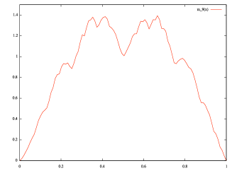
Figure 1. Graph of $f_{1}$ for $\displaystyle(b_{1}(t),c_{0}(t),c_{1}(t))=\left(t+\frac{1}{2},\ -\frac{1}{3},\ \frac{1}{3}\right)$.

6. Results for two special cases

We say (L) holds if $(b_{1}(t),c_{0}(t),c_{1}(t))=(t+a,0,0)$ for some $a\in(0,1)$. In this section we always assume (ND) holds and either $k=1$ or (L) holds. Recall Definition 5.2 and Lemma 5.3 for (ND).

Let

$$Y_{i}(x):=\frac{\partial_{t}H_{i-1}(0,x)}{H_{i-1}(0,x)},\,i\geq 1,\text{ and }Y_{0}(x):=0.$$

$Y_{i}(x)>0$ if and only if $X_{i}(x)=0$. If (L) holds,

$$Y_{i}(x)=\frac{1}{a}1_{\{X_{i}(x)=0\}}(x)+\frac{1}{1-a}1_{\{X_{1}(x)=1\}}(x).$$

Lemmas 2.5 and 5.3 imply

$$0<\inf_{i\geq 1,x\in(0,1)}|Y_{i}(x)|\leq\sup_{i\geq 1,x\in(0,1)}|Y_{i}(x)|<+\infty.$$ (6.1)

Recall the definition of $Z_{k,n}$ in (5.11). Then

$$Z_{1,n}(x)=\sum_{i=1}^{n}Y_{i}(x).$$ (6.2)

If (L) holds, using (5.15),

$$Z_{k,n+1}(x)-Z_{k,n}(x)=kY_{n+1}(x)Z_{k-1,n}(x),\ \ x\in[0,1),\ \ k\geq 2.$$ (6.3)

Let $\mu_{0}(\cdot|A)$ be the conditional probability of $\mu_{0}$ given a Borel measurable set $A$. Denote the expectation with respect to $\mu_{0}(\cdot|A)$ by $E^{\mu_{0}}_{A}$. Let

$$\mathcal{F}_{n}:=\sigma\left(\left\{\left[\frac{k}{2^{n}},\frac{k+1}{2^{n}}\right)\ \bigg{|}\ 0\leq k\leq 2^{n}-1\right\}\right),\ \ n\geq 0.$$

Then $\{Z_{k,i}\}_{i\geq n}$ is a $\{\mathcal{F}_{i}\}_{i}$-martingale with respect to $\mu_{0}(\cdot|A)$ for $A\in\mathcal{F}_{n}$. By induction on $k$

$$Z_{k,n}=k!\sum_{1\leq i_{1}<\cdots<i_{k}\leq n}\left(\prod_{j=1}^{k}Y_{i_{j}}\right)=O(n^{k}).$$

Lemma 6.1 (Fluctuation of $\{Z_{k,n}\}_{n}$).

For each $k\geq 1$

$$\limsup_{m\to+\infty}Z_{k,m}(x)>\liminf_{m\to+\infty}Z_{k,m}(x),\ \ x\in(0,1).$$ (6.4)

$$\limsup_{m\to\infty}E^{\mu_{0}}_{A}\left[\left|Z_{k,m}\right|\right]=+\infty,\ \ A\in\mathcal{F}_{n},n\geq 1.$$ (6.5)

Proof.

The case $k=1$ of (6.4) follows from (6.1). Assume (L) holds. We now show this by induction on $k$. Assume that this assertion holds for $k=1,\dots,l$ and

$$\limsup_{n\to+\infty}Z_{l+1,n}(x)=\liminf_{n\to+\infty}Z_{l+1,n}(x)\ \text{ for some $x$.}$$

Then (6.3) and (6.1) imply $\lim_{n\to\infty}Z_{l,n}(x)=0$. This contradicts the assumption of induction. Hence

$$\limsup_{n\to+\infty}Z_{l+1,n}(x)>\liminf_{n\to+\infty}Z_{l+1,n}(x)$$

for any $x$. Thus we have (6.4). Using this, (6.4) and the martingale convergence theorem ([15, Chapter 11]), we have (6.5). ∎

6.1. Differentiablity and variation

For $g:[0,1]\to\mathbb{R}$ and $0\leq a\leq b\leq 1$, let

$$V(g;[a,b]):=\sup\left\{\sum_{i=1}^{n}|g(t_{i})-g(t_{i-1})|\ \ \bigg{|}\ \ a=t_{0}<t_{1}<\cdots<t_{n}=b\right\}.$$

Theorem 6.2.

(i) $($Non-differentiablity for the absolutely continuous case$)$ For any $x\in(0,1)$, $\Delta_{k}F(x,x+h)$ does not converge to any real number as $h\to 0$. In particular, if $\mu_{0}$ is absolutely continuous, $f_{k}$ is not differentiable at any point in $(0,1)$.
(ii) $($Variation$)$ $V(f_{k};[a,b])=+\infty$ holds for any $[a,b]\subset[0,1]$, $a<b$.

(i) is an extension of [1, Theorem 5.1]. A problem of this kind was also considered by [14]. Our proof of (i) is somewhat similar to Billingsley [4] and [1, Theorem 5.1]. The key is a fluctuation of $\{Z_{k,n}\}_{n}$ in (6.4). It seems natural to consider whether $f_{k}$ is of bounded variation. To our knowledge variations of $f_{k}$ have not been considered. The key of proof of (ii) is showing, by using (6.5), the expectation of $\left|Z_{k,m}\right|$ under $\mu_{0}$ on an interval diverges to infinity.

Proof.

If $x\in D$, the assertion follows from Theorem 5.4 and the condition (ND). Assume $x\notin D$. It is easy to see that for any $k,n\geq 1$

$$\min\left\{\Delta_{k}F(x,x_{n}),\Delta_{k}F(x,x_{n}+2^{-n})\right\} \leq Z_{k,n}(x)$$

$$\leq\max\left\{\Delta_{k}F(x,x_{n}),\Delta_{k}F(x,x_{n}+2^{-n})\right\}$$ (6.6)

By (6.4) $Z_{k,n}(x)$ does not converge to any real number. Therefore if $(Z_{k,n}(x))_{n}$ diverges as $n\to+\infty$,

$$\limsup_{h\to 0}\left|\Delta_{k}F(x,x+h)\right|=+\infty.$$

If $(Z_{k,n}(x))_{n}$ fluctuates as $n\to+\infty$,

$$\limsup_{h\to 0}\Delta_{k}F(x,x+h)-\liminf_{h\to 0}\Delta_{k}F(x,x+h) \geq\limsup_{n\to+\infty}Z_{k,n}(x)-\liminf_{n\to+\infty}Z_{k,n}(x)$$

$$\geq c$$

for some $c=c(x)>0$. These imply (i). By (5.11),

$$\sum_{l=2^{m-n}(j-1)+1}^{2^{m-n}j}\left|f_{k}\left(\frac{l}{2^{m}}\right)-f_{k}\left(\frac{l-1}{2^{m}}\right)\right|=E^{\mu_{0}}_{[(j-1)/2^{n},j/2^{n})}\left[\left|Z_{k,m}\right|\right],\,m>n.$$

(ii) follows from this and (6.5). ∎

6.2. MTNI

Theorem 6.3 (MTNI).

For some $c\in[0,1]$ the following hold :
(i)

$$\ \ \ \ \ \ \ \ \ \ \ \ \ \ \ \ \limsup_{h\to 0}\frac{|f_{k}(x+h)-f_{k}(x)|}{|h|^{c}}=+\infty\ \ \text{ $\mu_{0}$-a.s.$x$.}\ \ \ \ \ \ \ \ \ \ \ \ \ \ \$$ (6.7)

(ii) For any open interval $J$

$$\ \ \sup_{x,y\in J,x>y}\frac{f_{k}(x)-f_{k}(y)}{(x-y)^{c}}=+\infty\ \text{ and }\inf_{x,y\in J,x>y}\frac{f_{k}(x)-f_{k}(y)}{(x-y)^{c}}=-\infty\ \$$

If $\mu_{0}$ is singular, $c<1$. If $\mu_{0}$ is absolutely continuous, $c=1$. If $(L)$ holds, $c$ does not depend on $k$.

(i) corresponds to Theorem 4.1 but here the limit diverges. If $\mu_{0}$ is singular, the asymptotic of $f_{k}$ around Lebesgue-a.e. points are quite different from the ones around $\mu_{0}$-a.s. points. (ii) extends [3, Theorem 14]. The proof of [3, Theorem 14] is omitted in [3]. However the reason that the proof of [3, Proposition 6] is not applied to even $k$ is not described in [3]. We will give a proof applied to all $k$ together.

For the proofs we first compare $\Delta_{k}F$ with $Z_{k,n}$ by (6.1) and then estimate $F(x_{n}+2^{-n})-F(x_{n})$ by (6.8) below. For (i) we will give a lower bound for $\left|f_{k}(x_{n}+2^{-n})-f_{k}(x_{n})\right|$ in terms of $|Z_{k,n}|$. Remark that $|Z_{k,n}|$ is positive by (6.4). For (ii), by probabilistic techniques we will choose $x$ such that $f_{k}(x_{n}+2^{-n})-f_{k}(x_{n})$ is “larger” than the positive part of $Z_{k,n}$, roughly speaking.

For $k=2$ we will give an example of graph of $f_{2}$ in Figure 2 below.

Proof.

By [10, Lemma 2.3 (2) and Lemma 3.3], there is a constant $c\leq 1$ such that

$$\limsup_{n\to\infty}\frac{-\log_{2}M_{n}(0,x)}{n}\leq c\text{ $\mu_{0}$-a.s.$x$.}$$ (6.8)

If $\mu_{0}$ is singular, $c<1$. If $\mu_{0}$ is absolutely continuous, $c=1$.

By (6.1) and (6.8)

$$\max\left\{\frac{\left|f_{k}(x)-f_{k}(x_{n})\right|}{(x-x_{n})^{c}},\frac{\left|f_{k}(x_{n}+2^{-n})-f_{k}(x)\right|}{(x_{n}+2^{-n}-x)^{c}}\right\}\geq\frac{1}{2}\left|Z_{k,n}(x)\right|,$$

for large $n$ and $\mu_{0}\text{-a.s.}x\in(0,1)\setminus D$. (6.4) implies

$$\limsup_{n\to\infty}|Z_{k,n}(x)|>0$$

holds for any $x$. Thus we have (i).

Fix $l$ and $n$. Denote $E^{\mu_{0}}_{[(l-1)/2^{n},l/2^{n})}$ by $E$. $Z_{k,m}^{+}$ and $Z_{k,m}^{-}$ denotes the positive and negative parts of $Z_{k,m}$. $Z_{k,m}^{+}-Z_{k,m}^{-}=Z_{k,m}$ and $Z_{k,m}^{+}+Z_{k,m}^{-}=|Z_{k,m}|$. Using (6.5) and that $\left\{\left|Z_{k,m}\right|\right\}_{m}$ is a submartingale,

$$\lim_{m\to\infty}E[Z_{k,m}^{+}]+E[Z_{k,m}^{-}]=\lim_{m\to\infty}E[|Z_{k,m}|]=\sup_{m}E[|Z_{k,m}|]=+\infty.$$

Since $\{Z_{k,m}\}_{m\geq n}$ is a martingale, $E[Z_{k,m}^{+}]-E[Z_{k,m}^{-}]=E[Z_{k,n}]$ for any $m\geq n$. Therefore

$$\lim_{m\to\infty}E[Z_{k,m}^{+}]=\lim_{m\to\infty}E[Z_{k,m}^{-}]=+\infty.$$ (6.9)

Let

$$A_{m}:=\left\{x:H_{m}(0,x)\leq 2^{-1-c_{1}m}\right\}.$$

By Azuma’s inequality ([15, Chapter E.14]) there are constants $c_{1}\in[0,1],c_{2},c_{3}\in(0,+\infty)$ such that for any $m$, $\mu_{0}(A_{m})\leq c_{2}\exp(-c_{3}m)$. This and (2.14) imply

$$E\left[Z_{k,m}^{+},A_{m}\right]\leq C_{k}m^{k}\frac{\mu_{0}(A_{m})}{\mu_{0}\left([(l-1)/2^{n},l/2^{n})\right)}\to 0,\,\,m\to\infty.$$

If $\left\{Z_{k,m}^{+}\geq E\left[Z_{k,m}^{+}\right]/2\right\}\subset A_{m}$ for large $m$,

$$\limsup_{m\to\infty}E\left[Z_{k,m}^{+}\right]\leq 2\limsup_{m\to\infty}E\left[Z_{k,m}^{+},A_{m}\right]=0.$$

This contradicts (6.9). Hence

$$\left\{Z_{k,m}^{+}\geq\frac{E[Z_{k,m}^{+}]}{2}\right\}\cap A_{m}^{c}\cap\left[\frac{l-1}{2^{n}},\frac{l}{2^{n}}\right)\neq\emptyset$$

holds for infinitely many $m$. Using this, (6.1) and (6.8), for $c$ in (6.8)

$$\sup_{x,y\in\left[(l-1)/2^{n},l/2^{n}\right],x>y}\frac{f_{k}(x)-f_{k}(y)}{(x-y)^{c}}=+\infty.$$ (6.10)

Since $\lim_{m\to\infty}E[Z_{k,m}^{-}]=+\infty$, there is $c\in[0,1]$ such that

$$\inf_{x,y\in\left[(l-1)/2^{n},l/2^{n}\right],x>y}\frac{f_{k}(x)-f_{k}(y)}{(x-y)^{c}}=-\infty.$$ (6.11)

(6.10) and (6.11) imply (ii). ∎

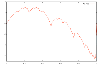
Figure 2. Graph of $f_{2}$ for $\displaystyle(b_{1}(t),c_{0}(t),c_{1}(t))=\left(t+\frac{1}{3},0,0\right)$.

7. Modulus of continuity

In this section we always assume (ND) holds and $k=1$. First we will give some notation and lemmas. Second we will compare $\Delta_{1}F(x,x+h)$ with $\log_{2}(1/|h|)$ for $x\notin D$. Finally we will consider a modulus of continuity for $\Delta_{1}F(x,x+h)$ at $\mu_{0}$-a.s.$x$.

Let

$$l(y,z):=\min\left\{i\geq 1:X_{i}(y)\neq X_{i}(z)\right\},\ \ y\neq z.$$

Recall (4.1) for the definition of $m_{1}(z)$.

Lemma 7.1 ([7, Lemma 2]).

Let $x\notin D$ and $h>0$. Then
(i) $\displaystyle\lim_{h\to 0,h>0}l(x,x+h)=+\infty$.
(ii) $l(x,x+h)\leq m_{1}(h)$.
(iii) $X_{i}(x)=X_{i}(x+h)$ for $1\leq i\leq l(x,x+h)-1$.
(iv) $X_{l(x,x+h)}(x)=0$ and $X_{l(x,x+h)}(x+h)=1$.
(v) $X_{i}(x)=1$ and $X_{i}(x+h)=0$ for $l(x,x+h)<i\leq m_{1}(h)-1$.

Define

$$l_{x}:=\min\left\{j>l(x,x+h):X_{j}(x)=0\right\}\text{ and }l_{x+h}:=\min\left\{j>l(x,x+h):X_{j}(x+h)=1\right\}.$$

We have

$$(x+h)_{l_{x+h}-1}=(x+h)_{l(x,x+h)}=x_{l_{x}-1}+2^{-(l_{x}-1)}.$$ (7.1)

Lemma 7.2 (Key lemma).

Let $x\notin D$ and $h>0$. Then

$$\Delta_{1}F(x,x+h) =\frac{F((x+h)_{l(x,x+h)})-F(x)}{F(x+h)-F(x)}Z_{1,l_{x}}(x)$$

$$+\frac{F(x+h)-F((x+h)_{l(x,x+h)})}{F(x+h)-F(x)}Z_{1,l_{x+h}}(x+h)+O(1).$$ (7.2)

Proof.

By (2.11)

$$f_{1}(x_{n+1})-f_{1}(x_{n})=X_{n+1}(x)\left(F(x_{n}+2^{-n-1})-F(x_{n})\right)\left(Z_{1,n}(x)+\overline{Y_{n}}(x)\right),$$

$$\text{where }\ \ \overline{Y_{n}}(x):=-\frac{H_{n}(0,x_{n}+2^{-n-1})}{H_{n}(0,x_{n})}Y_{n+1}(x_{n}+2^{-n-1}).$$

$\{\overline{Y_{n}}\}_{n}$ are bounded by (2.8) and (6.1). Summing up over $n$,

$$f_{1}(x)-f_{1}(x_{k})=(F(x)-F(x_{k}))Z_{1,k}(x)+J(x,k)$$

$$\text{where }\ J(x,k):=\sum_{n=k}^{\infty}X_{n+1}(x)\left(F(x_{n}+2^{-n-1})-F(x_{n})\right)\left(\sum_{i=k+1}^{n}Y_{i}(x)+\overline{Y_{n}}(x)\right).$$

(2.8) and (6.1) imply $J(x,k)=O\left(F(x_{k}+2^{-k})-F(x_{k})\right)$. Therefore

$$f_{1}(x+h)-f_{1}((x+h)_{l_{x+h}-1})=(F(x+h)-F((x+h)_{l_{x+h}-1}))\left(Z_{1,l_{x+h}}(x+h)+O(1)\right)\text{ and }$$

$$f_{1}(x)-f_{1}(x_{l_{x}-1})=(F(x)-F(x_{l_{x}-1}))Z_{1,l_{x}-1}(x)+O\left(F(x_{l_{x}-1}+2^{-(l_{x}-1)})-F(x_{l_{x}-1})\right).$$

(7.1) implies

$$f_{1}((x+h)_{l_{x+h}-1})-f_{1}(x_{l_{x}-1})=\left(F((x+h)_{l_{x+h}-1})-F(x_{l_{x}-1})\right)Z_{1,l_{x}-1}(x).$$

Therefore

$$f_{1}(x+h)-f_{1}(x) =\left(F((x+h)_{l_{x+h}-1})-F(x)\right)Z_{1,l_{x}}(x)$$

$$+\left(F(x+h)-F((x+h)_{l_{x+h}-1})\right)\left(Z_{1,l_{x+h}}(x+h)+O(1)\right)$$

$$+O\left(F(x_{l_{x}-1}+2^{-(l_{x}-1)})-F(x_{l_{x}-1})\right).$$

Since $F(x_{l_{x}-1}+2^{-(l_{x}-1)})-F(x_{l_{x}-1})=O\left(F(x+h)-F(x)\right)$ we have (7.2). ∎

7.1. Modulus of continuity at non-dyadic rationals

Recall (4.1) for the definition of $\{m_{n}(z)\}_{n}$.

Theorem 7.3.

Assume $x\notin D$. Then

$$\lim_{h\to 0,h>0}\frac{\Delta_{1}F(x,x+h)}{\log_{2}(1/h)}\text{ exists as a real number }$$

if and only if

$$\lim_{n\to\infty}\frac{m_{n+1}(1-x)}{m_{n}(1-x)}=1\text{ and }\lim_{n\to\infty}\frac{Z_{1,n}(x)}{n}\text{ exists.}$$

If they hold,

$$\lim_{h\to 0,h>0}\frac{\Delta_{1}F(x,x+h)}{\log_{2}(1/h)}=\lim_{n\to\infty}\frac{Z_{1,n}(x)}{n}.$$

Considering also the limit from left we have Corollary 7.6, which extends [2, Theorem 5.4]. [2] uses Kôno’s expression [7, Lemma 3]. If (L) holds then we may expect a counterpart of [7, Lemma 3]. However if (L) fails then it seems impossible to obtain a counterpart of [7, Lemma 3]. The key point is Lemma 7.2 above, which states $\Delta_{1}F(x,x+h)$ is between $Z_{1,l_{x}}(x)$ and $Z_{1,l_{x+h}}(x+h)$, roughly speaking. In Propositions 7.4 and 7.5 below we will investigate the asymptotic of $\Delta_{1}F(x,x+h)-Z_{1,l(x,x+h)}(x)$. These results are different depending on the asymptotic for $\dfrac{m_{n+1}(1-x)}{m_{n}(1-x)}$. Eliminate parts consisting of the differentials by estimating $Z_{1,l_{x}}(x)-Z_{1,l(x,x+h)}(x)$ and $Z_{1,l_{x+h}}(x+h)-Z_{1,l(x,x+h)}(x)$. Finally consider quantities expressed by $F$, $x$ and $h$ only as in (7.3) and (7.4) below.

Proposition 7.4.

If $x\notin D$ and $\displaystyle\lim_{n\to\infty}\dfrac{m_{n+1}(1-x)}{m_{n}(1-x)}=1$,

$$\lim_{h\to 0,h>0}\frac{\Delta_{1}F(x,x+h)-Z_{1,\lfloor\log_{2}(1/h)\rfloor}(x)}{\log_{2}(1/h)}=0.$$

Here $\lfloor x\rfloor$ denotes the maximal integer less than or equal to $x$.

Proof.

First we remark $\displaystyle\lim_{h\to 0,h>0}\frac{l(x,x+h)}{m_{1}(h)}=1$ by the assumptions. By (6.1), (6.2) and (7.2) it suffices to show

$$\lim_{h\to 0,h>0}\frac{F((x+h)_{l_{x+h}-1})-F(x)}{F(x+h)-F(x)}\cdot\frac{l_{x}-m_{1}(h)}{m_{1}(h)}=0\text{ and }$$ (7.3)

$$\lim_{h\to 0,h>0}\frac{F(x+h)-F((x+h)_{l_{x+h}-1})}{F(x+h)-F(x)}\cdot\frac{l_{x+h}-l(x,x+h)+m_{1}(h)-l(x,x+h)}{m_{1}(h)}=0.$$ (7.4)

Using Lemma 7.1 and $\displaystyle\lim_{n\to\infty}\dfrac{m_{n+1}(1-x)}{m_{n}(1-x)}=1$ we have (7.3).

We now show (7.4). We will give an upper bound for

$$(*):=\frac{F(x+h)-F((x+h)_{l_{x+h}-1})}{F(x+h)-F(x)}\times\left(\frac{l_{x+h}}{l(x,x+h)}-1\right).$$

If $l_{x+h}\leq(1+\epsilon)l(x,x+h)$, $(*)\leq\epsilon$.

Using (2.9) and

$$M_{l(x,x+h)-1}\left(0,(x+h)_{l_{x+h}-1}\right)=M_{l(x,x+h)-1}\left(0,x_{l_{x}}+2^{-l_{x}}\right),$$

there are constants $0<c<1\leq C<+\infty$ such that

$$\frac{F(x+h)-F((x+h)_{l_{x+h}-1})}{F(x+h)-F(x)} \leq\frac{M_{l_{x+h}-1}\left(0,(x+h)_{l_{x+h}-1}\right)}{M_{l_{x}}\left(0,x_{l_{x}}+2^{-l_{x}}\right)}$$

$$=C^{l_{x}-l(x,x+h)}c^{l_{x+h}-l(x,x+h)}$$

For any $\epsilon>0$ there is $\delta(\epsilon)>0$ with $c^{\epsilon/2}<C^{\delta(\epsilon)}$. Therefore if $l_{x+h}\geq(1+\epsilon)l(x,x+h)$ and $h$ is sufficiently small, $l_{x}\leq(1+\delta(\epsilon))l(x,x+h)$ and

$$\left(\frac{l_{x+h}}{l(x,x+h)}-1\right)\left(\frac{c^{l_{x+h}/l(x,x+h)-1}}{C^{l_{x}/l(x,x+h)-1}}\right)^{l(x,x+h)}\leq\frac{(l_{x+h}-l(x,x+h))c^{(l_{x+h}-l(x,x+h))/2}}{l(x,x+h)}.$$

Hence $(*)\leq\epsilon$. Thus we have (7.4). ∎

Proposition 7.5.

If $x\notin D$ and $\displaystyle\limsup_{n\to\infty}\dfrac{m_{n+1}(1-x)}{m_{n}(1-x)}>1$,

$$\frac{\Delta_{1}F(x,x+h)}{\log_{2}(1/h)}\text{ fluctuates if $h\to 0,h>0$. }$$

Proof.

Let $\delta>0$ and $(n(j))_{j}$ be an increasing sequence satisfying

$$m_{n(j)}(1-x)\geq m_{n(j)-1}(1-x)(1+\delta).$$

Assume $b_{1}(1+c_{0})(1+c_{1})\geq 1-b_{1}$. Let

$$m(1,j):=m_{n(j)}(1-x)-2\text{ and }m(2,j):=m_{n(j)}(1-x).$$

Then

$$F(x+2^{-m(1,j)})-F(x)\leq M_{m(1,j)}(0,x_{m(1,j)})+M_{m(1,j)}\left(0,x_{m(1,j)}+2^{-m(1,j)}\right),$$ (7.5)

$$F(x+2^{-m(1,j)})-F\left((x+2^{-m(1,j)})_{m(1,j)}\right)\geq M_{m(1,j)}\left(0,x_{m(1,j)}+2^{-m(1,j)}\right)\text{ and }$$ (7.6)

$$\frac{M_{m(1,j)}\left(0,x_{m(1,j)}+2^{-m(1,j)}\right)}{M_{m(1,j)}(0,x_{m(1,j)})}=\prod_{i=m_{n(j)-1}(1-x)}^{m_{n(j)}(1-x)-1}\frac{H_{i}\left(0,x_{m(1,j)}+2^{-m(1,j)}\right)}{H_{i}(0,x_{m(1,j)})}.$$ (7.7)

By Lemma 5.2 (i) and $m_{n(j)}(1-x)-m_{n(j)-1}(1-x)\geq(1+\delta)j$,

$$\lim_{j\to\infty}\prod_{i=m_{n(j)-1}(1-x)}^{m_{n(j)}(1-x)-1}\frac{H_{i}\left(0,x_{m(1,j)}+2^{-m(1,j)}\right)}{b_{1}(c_{0}+1)}=1.$$ (7.8)

$$\lim_{j\to\infty}\prod_{i=m_{n(j)-1}(1-x)}^{m_{n(j)}(1-x)-1}\frac{H_{i}(0,x_{m(1,j)})(1+c_{0})}{1-b_{1}}=1.$$ (7.9)

Using (7.5), (7.6), (7.7), (7.8), (7.9) and $b_{1}(1+c_{0})(1+c_{1})\geq 1-b_{1}$,

$$\liminf_{j\to\infty}\frac{F(x+2^{-m(1,j)})-F\left((x+2^{-m(1,j)})_{m(1,j)}\right)}{F(x+2^{-m(1,j)})-F(x)}\geq\frac{1}{2}.$$ (7.10)

Since

$$m(1,j)-l(x,x+2^{-m(1,j)})=m_{n(j)}(1-x)-m_{n(j)-1}(1-x)-2,$$

$$\liminf_{j\to\infty}\frac{m(1,j)-l(x,x+2^{-m(1,j)})}{m(1,j)}>0.$$

Using this, (7.10) and (7.2),

$$\liminf_{j\to\infty}\frac{\Delta_{1}F(x,x+2^{-m(1,j)})-Z_{1,m(1,j)}(x)}{m(1,j)}>0.$$ (7.11)

Recall $m(2,j)=l(x,x+2^{-m(2,j)})$ and (7.2). Considering the cases $X_{m(2,j)}(x)=0$ and $X_{m(2,j)}(x)=1$ respectively,

$$\limsup_{j\to\infty}\frac{\Delta_{1}F(x,x+2^{-m(2,j)})-Z_{1,m(2,j)}(x)}{m(2,j)}\leq 0.$$ (7.12)

By (6.1),

$$\lim_{j\to\infty}\frac{Z_{1,m(1,j)}(x)}{m(1,j)}-\frac{Z_{1,m(2,j)}(x)}{m(2,j)}=0.$$ (7.13)

Using (7.11), (7.12) and (7.13), we have the assertion.

If $b_{1}(1+c_{0})(1+c_{1})<1-b_{1}$, by Lemma 5.1 (ii) there are $c^{\prime},c^{\prime\prime}>0$ and $\delta_{1},\delta_{2}\in(0,\delta)$ such that for large $j$

$$\Delta_{1}F\left(x,x+2^{-(1+\delta_{1})n(j-1)}\right)\geq Z_{1,n(j-1)}(x)+c^{\prime}\delta_{1}n(j-1)\text{ and }$$

$$\Delta_{1}F\left(x,x+2^{-(1+\delta_{2})n(j-1)}\right)\leq Z_{1,n(j-1)}(x)-c^{\prime\prime}\delta_{2}n(j-1).$$

For large $j$,

$$\frac{\Delta_{1}F\left(x,x+2^{-(1+\delta_{1})n(j-1)}\right)}{(1+\delta_{1})n(j-1)}-\frac{\Delta_{1}F(x,x+2^{-n(j-1)})}{n(j-1)}\geq\frac{c^{\prime}}{2}\delta_{1}\,\text{ if $Z_{1,n(j-1)}(x)<0$.}$$

$$\frac{\Delta_{1}F\left(x,x+2^{-(1+\delta_{2})n(j-1)}\right)}{(1+\delta_{2})n(j-1)}-\frac{\Delta_{1}F(x,x+2^{-n(j-1)})}{n(j-1)}\leq-\frac{c^{\prime\prime}}{2}\delta_{2}\,\text{ if $Z_{1,n(j-1)}(x)>0$. }$$

Thus we have the assertion. ∎

Theorem 7.3 follows from Propositions 7.4 and 7.5.

Note

$$\Delta_{1}F(x,x+h)=\Delta_{1}\widetilde{F}(1-x,1-x-h)\text{ and }\widetilde{Z}_{1,n}(1-x)=Z_{1,n}(x),\ \ x\notin D.$$

We can consider $\displaystyle\lim_{h\to 0,h<0}\dfrac{\Delta_{1}F(x,x+h)}{\log_{2}(1/|h|)}$ in the same manner. We have

Corollary 7.6.

Assume $x\notin D$. Then

$$\lim_{h\to 0}\frac{\Delta_{1}F(x,x+h)}{\log_{2}(1/|h|)}\text{ exists }$$

if and only if

$$\lim_{n\to\infty}\frac{m_{n+1}(1-x)}{m_{n}(1-x)}=\lim_{n\to\infty}\frac{m_{n+1}(x)}{m_{n}(x)}=1\text{ and }\lim_{n\to\infty}\frac{Z_{1,n}(x)}{n}\text{ exists.}$$

7.2. Modulus of continuity at $\mu_{0}$-a.s. points

Theorem 7.7.

There are two constants $0<c\leq C<+\infty$ such that the following hold for $\mu_{0}$-a.s. $x$ :

$$c\leq\limsup_{h\to 0}\frac{\Delta_{1}F(x,x+h)}{(\log_{2}(1/|h|)\log\log\log_{2}(1/|h|))^{1/2}}\leq C.$$ (7.14)

$$-C\leq\liminf_{h\to 0}\frac{\Delta_{1}F(x,x+h)}{(\log_{2}(1/|h|)\log\log\log_{2}(1/|h|))^{1/2}}\leq-c.$$ (7.15)

By this we can improve (6.7) for $k=1$ as follows :

$$\limsup_{h\to 0}\frac{f_{1}(x+h)-f_{1}(x)}{|h|^{c}}=+\infty=-\liminf_{h\to 0}\frac{f_{1}(x+h)-f_{1}(x)}{|h|^{c}}\text{ $\mu_{0}$-a.s.$x$.}$$

As we will see in Corollaries 7.9 and 7.10, for some special choices of $(b_{1}(t),c_{0}(t),c_{1}(t))$, we can improve (7.14) and (7.15).

The key tools of the lower bound for (7.14) and the upper bound for (7.15) are (6.1) and Stout’s law of the iterated logarithm (LIL) below. Recall (6.2). Apply Stout’s law of the iterated logarithm (LIL) below to $\{Y_{i}\}_{i}$. The key tool of the upper bound for (7.14) and the lower bound for (7.15) is Lemma 7.2 above, which states $\Delta_{1}F(x,x+h)$ is between $Z_{1,l_{x}}(x)$ and $Z_{1,l_{x+h}}(x+h)$, roughly. Estimate parts consisting of the differentials by estimating $Z_{1,l_{x}}(x)-Z_{1,l(x,x+h)}(x)$ and $Z_{1,l_{x+h}}(x+h)-Z_{1,l(x,x+h)}(x)$. Now apply Stout’s LIL to $Z_{1,l(x,x+h)}(x)$ and these differences.

Lemma 7.8 (Stout’s LIL for martingales [13]).

Let $(\Omega,\mathcal{F},P)$ be a probability space and $\{S_{n},\mathcal{F}_{n}\}_{n\geq 0}$ be a martingale on it. Let $I_{n}:=\sum_{i=1}^{n}E[(S_{i}-S_{i-1})^{2}|\mathcal{F}_{i-1}]$ where we denote the expectation with respect to $P$ by $E$. Assume there are constants $0<c\leq C<+\infty$ such that $c\leq|S_{i}-S_{i-1}|\leq C$ $\mu_{0}$-a.s. for any $i\geq 1$. Then

$$\limsup_{n\to\infty}\frac{S_{n}}{(I_{n}\log\log I_{n})^{1/2}}=\sqrt{2}=-\liminf_{n\to\infty}\frac{S_{n}}{(I_{n}\log\log I_{n})^{1/2}}\ \text{ $P$-a.s.}$$

Proof of Theorem 7.7.

First we show the lower bound for (7.14) and the upper bound for (7.15). Recall (6.1). Applying Lemma 7.8 to $\{Y_{i}\}_{i}$, there is $c>0$ such that the following hold $\mu_{0}$-a.s.$x$ :

$$\limsup_{n\to+\infty}\frac{\max\left\{\Delta_{1}F(x,x_{n}),\Delta_{1}F(x,x_{n}+2^{-n})\right\}}{(n\log\log n)^{1/2}}\geq c.$$ (7.16)

$$\liminf_{n\to+\infty}\frac{\min\left\{\Delta_{1}F(x,x_{n}),\Delta_{1}F(x,x_{n}+2^{-n})\right\}}{(n\log\log n)^{1/2}}\leq-c.$$ (7.17)

By [10, Lemma 3.2] there are constants $0<c^{\prime}\leq c^{\prime\prime}<1$ such that

$$c^{\prime}\leq\liminf_{n\to+\infty}\frac{\left|\{i\in\{1,\dots,n\}:X_{i}(x)=0\}\right|}{n}\leq\limsup_{n\to+\infty}\frac{\left|\{i\in\{1,\dots,n\}:X_{i}(x)=0\}\right|}{n}\leq c^{\prime\prime}$$

holds $\mu_{0}$-a.s. $x$.

Let $\sigma(h):=\log_{2}\left(1/|h|\right)$ for $h\neq 0$. Using this and (6.1), there is $C<+\infty$ such that

$$\limsup_{n\to\infty}\frac{\sigma(x-x_{n})+\sigma(x_{n}+2^{-n}-x)}{\sigma(2^{-n})}\leq C\text{ $\mu_{0}$-a.s.$x$.}$$ (7.18)

(7.16) and (7.18) imply the lower bound for (7.14). (7.17) and (7.18) imply the upper bound for (7.15).

Second we show the upper bound for (7.14) and the lower bound for (7.15). Assume $h>0$. Applying Lemma 7.8 to $\left\{\sum_{i=1}^{n}X_{i}-E^{\mu_{0}}[X_{i}|\mathcal{F}_{i-1}]\right\}_{n}$ and $\{Y_{i}\}_{i}$,

$$l_{x}-l(x,x+h)+l_{x+h}-l(x,x+h)=O\left((l(x,x+h)\log\log l(x,x+h))^{1/2}\right)\text{ and }$$

$$Z_{1,l(x,x+h)}(x)=O\left((l(x,x+h)\log\log l(x,x+h))^{1/2}\right),h\to 0,h>0,\text{ $\mu_{0}$-a.s.$x$.}$$

Using (7.2)

$$\Delta_{1}F(x,x+h)=O\left((\sigma(h)\log\log\sigma(h))^{1/2}\right),\,h\to 0,h>0,\text{ $\mu_{0}$-a.s.$x$.}$$ (7.19)

Now assume $h<0$. Applying Lemma 7.8 to $\{\widetilde{Y}_{i}\}_{i}$,

$$\Delta_{1}\widetilde{F}(y,y+h)=O\left((\sigma(h)\log\log\sigma(h))^{1/2}\right),\,h\to 0,h>0,\text{ $\widetilde{\mu}_{0}$-a.s.$y$.}$$

Let $T(y):=1-y$. By (2.4), $\widetilde{\mu}_{0}=\mu_{0}\circ T^{-1}\text{ and }$

$$\Delta_{k}\widetilde{F}(x,y)=\Delta_{k}F(1-x,1-y),\ \ x,y\in(0,1),\,k\geq 1.$$ (7.20)

Therefore

$$\Delta_{1}F(x,x+h)=\Delta_{1}\widetilde{F}(1-x,1-x-h)=O\left((\sigma(h)\log\log\sigma(h))^{1/2}\right),\,h\to 0,h<0,\text{ $\mu_{0}$-a.s.$x$.}$$ (7.21)

(7.19) and (7.21) complete the proof of the upper bound for (7.14) and the lower bound for (7.15). ∎

Let

$$I_{n}(x):=\sum_{i=1}^{n}E\left[Y_{i}^{2}|\mathcal{F}_{i-1}\right](x)\text{ and }\sigma(h,x):=I_{\lfloor\log_{2}(1/|h|)\rfloor}(x).$$

Corollary 7.9.

If $\mu_{0}$ is absolutely continuous,

$$\liminf_{h\to 0}\frac{\Delta_{1}F(x,x+h)}{\left(\sigma(h,x)\log\log\sigma(h,x)\right)^{1/2}}=-\sqrt{2}\ \ \ \text{ $\mu_{0}$-a.s. $x$.}$$ (7.22)

Proof.

Assume $x\notin D$ and $h>0$. Using Lemma 7.2 and that

$$Z_{1,l_{x+h}}(x+h)\geq Z_{1,l(x,x+h)}(x+h)=Z_{1,l(x,x+h)}(x)+O(1),$$

$$\Delta_{1}F(x,x+h)\geq\min\left\{Z_{1,l_{x}}(x),Z_{1,l(x,x+h)}(x)\right\}+O(1).$$

Since $\displaystyle\lim_{h\to 0,h>0}\dfrac{l_{x}}{l(x,x+h)}=1$,

$$\lim_{h\to 0,h>0}\frac{I_{l(x,x+h)}(x)}{\sigma(h,x)}=\lim_{h\to 0,h>0}\frac{I_{l_{x}}(x)}{\sigma(h,x)}=1\ \ \ \text{ $\mu_{0}$-a.s.$x$. }$$

Therefore

$$\liminf_{h\to 0,h>0}\frac{\Delta_{1}F(x,x+h)}{\left(\sigma(h,x)\log\log\sigma(h,x)\right)^{1/2}}\geq-\sqrt{2}\ \ \ \text{ $\mu_{0}$-a.s.$x$.}$$

By (7.20)

$$\liminf_{h\to 0,h<0}\frac{\Delta_{1}F(x,x+h)}{\left(\sigma(h,x)\log\log\sigma(h,x)\right)^{1/2}}\geq-\sqrt{2}\ \ \ \text{ $\mu_{0}$-a.s.$x$}$$

in the same manner. Thus we have

$$\liminf_{h\to 0}\frac{\Delta_{1}F(x,x+h)}{\left(\sigma(h,x)\log\log\sigma(h,x)\right)^{1/2}}\geq-\sqrt{2}\ \ \ \text{ $\mu_{0}$-a.s.$x$.}$$

If $\mu_{0}$ is absolutely continuous,

$$\lim_{n\to\infty}\frac{\sigma(x-x_{n},x)}{I_{n}(x)}=\lim_{n\to\infty}\frac{\sigma(x_{n}+2^{-n}-x,x)}{I_{n}(x)}=1\ \ \ \text{ $\mu_{0}$-a.s.$x$.}$$

Using this, Lemma 7.8 and (6.1), we have the upper bound of (7.22). ∎

If $b_{1}(t)=t+\dfrac{1}{2}$ and $c_{0}(t)=c_{1}(t)=0$, by symmetry,

$$\partial_{t}F(0,x)=\partial_{t}F(0,1-x),F(x)=1-F(1-x)\text{ and }\sigma(h,x)=\lfloor\log_{2}(1/|h|)\rfloor.$$

Hence

Corollary 7.10 (The original Takagi function case of [7, Theorem 5]).

If $b_{1}(t)=t+\dfrac{1}{2}$ and $c_{0}(t)=c_{1}(t)=0$, the following hold $\mu_{0}$-a.s. $x$ :

$$\limsup_{h\to 0}\frac{\Delta_{1}F(x,x+h)}{\left(\log_{2}(1/|h|)\log\log\log_{2}(1/|h|)\right)^{1/2}}=\sqrt{2}=-\liminf_{h\to 0}\frac{\Delta_{1}F(x,x+h)}{\left(\log_{2}(1/|h|)\log\log\log_{2}(1/|h|)\right)^{1/2}}.$$

References

- [1] P. C. Allaart and K. Kawamura, Extreme values of some continuous, nowhere differentiable functions, Math. Proc. Camb. Phil. Soc. 140 (2006), no. 2, 269-295.
- [2] P. C. Allaart and K. Kawamura, The improper infinite derivatives of Takagi’s nowhere-differentiable function, J. Math. Anal. Appl. 372 (2010), no. 2, 656-665.
- [3] E. de Amo, M. Díaz Carrillo and J. Fernández-Sánchez, Singular functions with applications to fractal dimensions and generalized Takagi functions, Acta Appl. Math. 119 (2012), 129-148.
- [4] P. Billingsley, Van der Waerden’s continuous nowhere differentiable function, Amer. Math. Monthly 89 (1982), 691.
- [5] J. B. Brown, U. B. Darji and E. P. Larsen, Nowhere monotone functions and functions of nonmonotonic type, Proc. Am. Math. Soc. 127(1), (1999) 173-182.
- [6] M. Hata and M. Yamaguti, The Takagi Function and Its Generalization, Japan J. Appl. Math. 1 (1984) 183-199.
- [7] N. Kôno, On generalized Takagi functions, Acta Math. Hung. 49 (1987), 315-324.
- [8] M. Krüppel, On the extrema and the improper derivatives of Takagi’s continuous nowhere differentiable function, Rostock. Math. Kolloq. 62 (2007), 41-59.
- [9] R. Mauldin and S. Williams, On the Hausdorff dimension of some graphs, Trans. Amer. Math. Soc. 298 (1986), 793-803.
- [10] K. Okamura, Singularity results for functional equations driven by linear fractional transformations, J. Theoret. Probab. 27 (2014) 1316-1328.
- [11] J. Paradís, P. Viader and L. Bibiloni, Riesz-Nágy singular fnuctions revisited, J. Math. Anal. Appl. 329 (2007) 592-602.
- [12] G. de Rham, Sur quelques courbes définies par des équations fonctionalles, Univ. e Politec. Torino. Rend. Sem. Mat. 16 (1957), 101-113.
- [13] W. F. Stout, A Martingale analogue of Kolmogorov’s law of the iterated logarithm, Z. Wahrscheinlichkeitstheorie und Verw. Gebiete 15 (1970), 279-290.
- [14] T. Takagi, A simple example of the continuous function without derivative, Phys.-Math. Soc. Japan 1 (1903), 176-177. The Collected Papers of Teiji Takagi, S. Kuroda, Ed., Iwanami (1973), 5-6.
- [15] D. Williams, Probability with martingales, Cambridge University Press, 1991.