Delocalization in One-Dimensional Tight-Binding Models with Fractal Disorder

Abstract

In the present work, we investigated the correlation-induced localization-delocalization transition in the one-dimensional tight-binding model with fractal disorder. We obtained a phase transition diagram from localized to extended states based on the normalized localization length by controlling the correlation and the disorder strength of the potential. In addition, the transition of the diffusive property of wavepacket dynamics is shown around the critical point.

1 Introduction

In some kinds of one-dimensional Schr$\ddot{o}$dinger operators with random potential, the eigenstates are mathematically proven to be localized ishii73 ; lifshiz88 ; stollmann01 . The one-dimensional tight-binding models with an ergodic and stationary random potential have positive Lyapunov exponent of the wavefunction with probability 1 (G-M-P theorem) goldsheid77 . The existence of the positive Lyapunov exponent is necessary and sufficient condition for a pure point set spectrum of the operators, and then all the eigenfunctions exhhibit the exponentially decay in the thermodynamic limit. Kotani’s theory states that if the potential sequence is nondeterministic under the following conditions, (i)stationarity, (ii)ergodicity, (iii) integrability, then there is no absolutely continuous (a.c.) spectrum of the operators kotani82 . These theorems can be proven true for continuous and discrete one-dimensional disordered systems (1DDS) simon83 ; kotani86 ; damanik04 . However, the necessary and sufficient condition for the exponential localization has not been found yet.

There is a possibility that the correlation effect of the potential sequence breaks the strong exponential localization and generates a localization-delocalization transition (LDT) in the 1DDS. Indeed, many authors numerically observed the correlation-induced LDT by using the some potential sequences with power spectrum $S(f)\sim 1/f^{\alpha}$($\alpha\geq 2$) as a potential by Fourier filtering method (FFM), where $f$ denotes frequency moura98 ; izrailev99 ; gong10 ; deng12 ; kaya07 ; gong12 ; albrecht12 . Such a potential obviously breaks a necessary condition (i), i.e. it is nonstationary. Note that the non-stationarity can be satisfied for $\alpha\geq 1$. In addition, the LDT with mobility edges, has been found numerically for the one-dimensional tight-binding model with the FFM model as the potential strength $W$ decreases bocker05 ; oliveira01 ; shima04 ; greis81 ; garcia09 ; garcia10 ; costa11 .

Shima et al and Kaya also showed that the 1DDS with FFM potential have a critical disorder strength $W_{c}$ separating the conducting and insulating phases, and the $W_{c}$ is independent of the spectrum index $\alpha(>2)$ shima04 ; kaya07 . Petercen and Sandler insisted that effect of the anticorrelation is also important to understand the transition due to the correlation of the sequence petersen13 .

On the other hand, the LDT due to the differentiability of the potential function also exists without contradiction with the Kotani’s theory. Very recently, Garcia and Cuevas studied the transition based on the differentiability of the disorder potential as a necessary condition for the delocalization garcia09 ; garcia10 . A certain degree of differentiability assures that the potential in neighboring sites is strongly correlated. They modeled the sequences with power-law spectrum by Weierstrass function with fractal dimension $D$. As a result they also numerically suggested that the transition takes place at the critical value $D_{c}=3/2$ by means of the distribution of the energy level-spacing in the weak disorder limit. However, studying the effect of the disorder strength in the 1DDS with the Weierstrass-type potential has been still unclarified.

In this paper, we have numerically studied the correlation-induced localization-delocalization transition by using tight-binding model with Weierstrass potential used by Garcia and Guevas garcia10 . The finite-size scaling analysis for the normalized localization length at band center numerically suggests the existence of the transition around $D\simeq 3/2$ independent of the potential strength in the relatively weak disorder regime. On the other hand, in the relatively strong disorder regime, the critical fractal dimension $D_{c}$ becomes smaller value than $D=3/2$ dependently on the potential strength. Furthermore, we have investigated the quantum diffusion of the initially localized wavepacket in the system. The transition from the localized state to ballistic states occurs around $D\simeq 3/2$ without scale invariant subdiffusive behavior.

This paper is organized as follows. In the next section, we introduce the 1DDS with the Weierstrass potential and some preliminary calculations. In Sect.3, we present global behavior of the $W-$dependence and $D-$dependence in the LDT by the numerical calculation of the normalized localization length. A phase diagram in the $D-W$ space is also given. In Sect.4, we show that the dynamical property of the system ought to be represented by the time dependence of the degree to which the initially localized wavepacket would be spread. Summary and discussion are presented in the last section. In an appendix, we give the behavior of the autocorrelation functions for the potential sequence.

2 Model and preliminary calculation

2.1 model

We consider the one-dimensional tight-binding model describing single-particle electronic states in the site representation as

$$u(n-1)+u(n+1)+WV(n)u(n)=Eu(n),$$ (1)

where $E$ and $\{u(n)\}_{n=0}^{N}$ are the energy and state of the system, respectively. The $\{V(n)\}_{n=0}^{N}$ and $W$ are the on-site energy sequence and the strength, respectively. To model the correlated and non-differential disorder potential for $V(n)$($n\leq N$) in Eq.(1), we use the following form:

$$V(n)=C\sum_{k=0}^{L}\frac{\sin(2\pi a^{k}n/N+\phi_{k})}{a^{(2-D)k}},$$ (2)

where $a$ is a constant value ($a>1$) related the scale-invariance and $D$ is a fractal dimension ($1<D<2$). $\{\phi_{k}\}_{k=0}^{L}$ are random independent variables chosen in the interval $[0,2\pi]$. $C$ is the normalization constant which is determined by a condition

$$\sqrt{<V(n)^{2}>-<V(n)>^{2}}=1,$$ (3)

where $\langle...\rangle$ indicates the average over realization of the phases in Eq.(2).

If we set $n/N=x$, $\phi_{k}=0$, the potential sequence becomes ”Weierstrass function” with continuous and indifferentiable everywhere by taking a continuous limit $N\to\infty$ and $L\to\infty$. Therefore, the potential will be shortly transfered to as ”Weierstrass potential” in this paper, and we set $a=2$ and $L=50$ thorough this paper without loss of the generality and accuracy of the numerical calculation. The power spectrum $S(f)$ of the Weierstrass function is empirically characterized by the fractal dimension $D$ as,

$$S(f)\sim\frac{1}{f^{5-2D}}.$$ (4)

In compassion with the form $S(f)\sim 1/f^{\alpha}$,

$$D=1+\frac{3-\alpha}{2}.$$ (5)

Note that the condition $\alpha\geq 2$ for the LDT in the FFM potential moura98 ; shima04 ; kaya07 corresponds to a condition $D\leq 3/2$. Increasing $\alpha$ corresponds to increasing correlations up to long-range correlated disorder. The analytical property of the autocorrelation function for the Weierstrass potential $V(n)$ is given in appendix A. It is found that the correlation linearly decreases from 1 for $D=3/2$.

In addition to the long-rang correlation, the fractal dimension $D$ also controls the degree of the differentiability of the potential function. The degree of the differentiability increases along with the decrease of the fractal dimension $D$. The smoothness of the potential fluctuation can also induce the delocalization of the quantum states, which property is directly related to analyticity of the potential function in the continuum limit, as pointed out by Garcia and Cuevas garcia09 ; garcia10 . They have numerically found that LDT at $D_{c}=3/2$ for the sufficiently weak disorder regime by using the nearest-neighbor level-space distribution of the energy spectrum. The result is not at odds with Kotani’s theory because the Weierstrass potential become non-stationary for $1<D\leq 3/2$.

2.2 preliminary calculation

The finite size Lyapunov exponent $\gamma_{N}(N>>1)$ of the one-dimensional systems can be defined by

$$\gamma_{N} = \frac{\ln\left(|u(N)|^{2}+|u(N+1)|^{2}\right)}{2N},$$ (6)

with initial state $u(0)=u(1)=1$. Then the Lyapunov exponent $\gamma$ and the localization length $\xi$ are given by $\gamma=\lim_{n\to\infty}\gamma_{N}$ and by $\xi=1/\gamma$, respectively. The energy dependence of $\gamma$ is strongly correlated with the density of states that can be obtained from some experiments for real materials. In addition, we define the normalized localization length (NLL),

$$\Lambda_{N}\equiv\frac{\xi(N)}{N}=\frac{1}{<\gamma_{N}>N},$$ (7)

, where $\langle...\rangle$ denotes the ensemble average. It is useful to study the LDT that $\Lambda_{N}$ decreases (increases) with the system size $N$ for localized (extended) states, and it becomes constant for the critical states.

Figure 1(a) shows the energy dependence of the Lyapunov exponent $\gamma_{N}$ for some values of the fractal dimension $D$. The Lyapunov exponent $\gamma_{N}$ at the band center $E=0$ decreases as the value of the $D$ decreases. It suggests a possibility of the delocalized states (extended states) at the band center $E=0$ for small values of $D(\leq 3/2)$. Figure 1(b) and (c) show the potential strength dependence of the Lyapunov exponent $<\gamma_{N}>$ and the renormalized localization length $\Lambda_{N}$ at the band center $E=0$ for some parameter sets. In the weak disorder regime $W<<1$, the numerical data lead to

$$\gamma_{N}\propto W,$$ (8)

despite of the system size, which is equivalent to case of the uncorrelated disordered system. In the strong disorder regime, the Lyapunov exponent does not depend on the system size $N$. Figure 1(c) shows the $W-$dependence of the NLL $\Lambda_{N}$. It is found that the localization length is larger than system size in the week disorder limit. The results suggest that for the strongly correlated limit, there is a possibility of the states with $<\gamma_{N}>\to 0$ and/or $\Lambda_{N}>1$ in the thermodynamic limit $N\to\infty$, which correspond to a delocalized phase with the extended states in week disorder limit. In the following section, we numerically investigate the $D-$dependence, $W-$dependence and $N-$dependence of the NLL in the 1DDS with the potential (2).

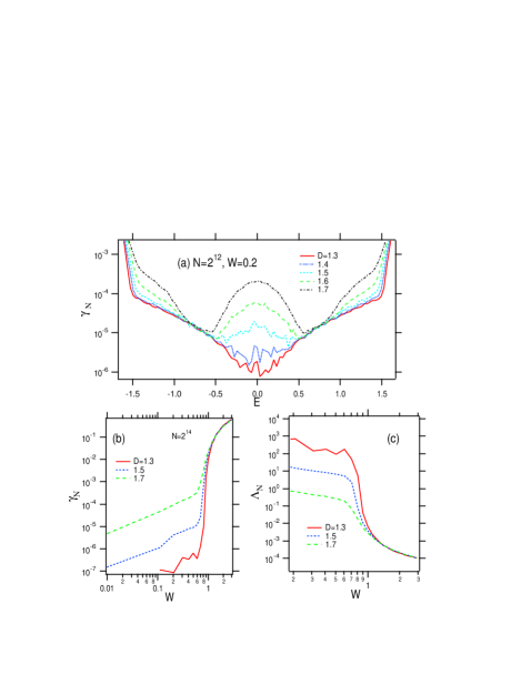
Figure 1: (Color online) (a)The Lyapunov exponent $\gamma_{N}$ as a function of energy $E$ for a weak disorder case, $W=0.2$ and varying the fractal dimension $D$. The system and ensemble sizes are $N=2^{12}$ and $2^{10}$, respectively. (b)The Lyapunov exponent $\gamma_{N}$ and (c)normalized localization length $\Lambda_{N}$ at the band center $E=0$ as a function of the potential strength $W$ for the several values of the $D$. This system and ensemble sizes are $N=2^{14}$ and $2^{10}$, respectively.

3 Localization-Delocalization Transition

This is the main section of the present paper. In what follows, we investigate the NLL at band center $E=0$ by changing the system size for some typical parameter sets ($W$,$D$). The typical basis size $N$ and ensemble size used here are $N=2^{8}\sim 2^{17}$ and $2^{10}\sim 2^{12}$, respectively. The robustness of the numerical calculations with respect to the system size has been confirmed in each case.

3.1 $D$-dependence and $W$-dependence in the wide parameters space

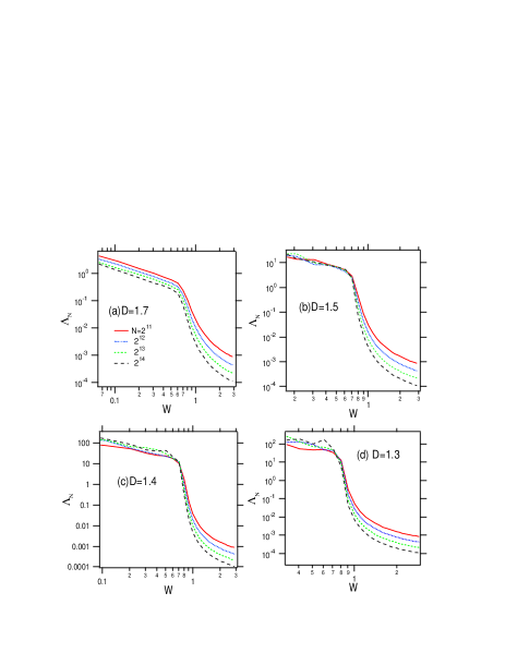
Figure 2: (Color online) The normalized localization length $\Lambda_{N}$ as a function of the potential strength $W$ with a fixed value of D for $N=2^{11},2^{12},2^{13},2^{14},2^{15},2^{16}$. (a)$D=1.7$, (b)$D=1.5$, (c)$D=1.4$, (d)$D=1.3$. Note that the data are plotted in double-logarithmic scale.

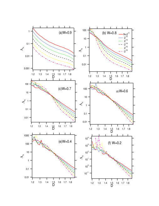
Figure 3: (Color online) The normalized localization length $\Lambda_{N}$ as a function of $D$ with a fixed value of W for $N=2^{11},2^{12},2^{13},2^{14},2^{15},2^{16}$. (a)$W=0.9$, (b)$W=0.8$, (c)$W=0.7$, (d)$W=0.6$, (e)$W=0.4$, (f)$W=0.2$. Note that the vertical axis are in logarithmic scale.

Figure 2 shows $W-$dependence of the NLL for some values of the $D$ in the relatively wide range. The $W-$dependence relatively smoothly drops down around $W\sim 1$ in the same way for all cases with different system size. There exists the strong system size dependence for the strong disorder regime $W>1$. Furthermore it is found that there is a quite different feature between the cases for $D<3/2$ and ones for $D>3/2$. In the case of $D=1.7$, the curve of the $W-$dependence for the different system size ($N=2^{11}\sim 2^{14}$) do not cross within this regime of $W$ with each others. This fact implies that all states around $E=0$ are localized in the thermodynamic limit and there is no transition for changing the value of $W$. On the other hand, in the cases of $D\leq 3/2$, the system size dependence for weak disorder regime $W<1$ becomes very weak, and the $W-$dependence sharply decreases at certain value of $W$. Apparently, we can expect that for $D\leq 3/2$ the $W-$dependence of the NLL shows a sharp jump in the thermodynamic limit $N\to\infty$. This feature suggests the existence of a transition to delocalized states in the limit $N\to\infty$.

In Fig.3 we show the $D-$dependence of the NLL for some values of $W$ in order to find out the critical value $D_{c}$ that all curves of different system size intersect at the value. At least, the existence of the intersection corresponding to a transition point can be observed around $D=3/2$ for the relatively weak disorder strength $W\leq 0.7$.

In the following two subsections, we investigate the details of the LDT with focusing on the relatively weak disorder regime ($W\leq 0.7$) and the relatively strong disorder regime ($0.7<W<0.8$), respectively.

3.2 Weak disorder regime

Figure 4(a) shows the system size dependence of the NLL for a relatively weak disorder strength $W=0.4$. It is found that the $N-$dependence changes the decreasing function to the increasing function as the fractal dimension decreases, and the $N-$dependences are algebraic. Generally, the quantum states can be classified by the exponent $\delta$ of the $N-$dependence of the NLL $\Lambda_{N}$ when it behaves as,

$$\Lambda_{N}\sim N^{\delta}.$$ (9)

The exponent, $\delta<0$ for the localized states, $\delta>0$ for the extended states, and $\delta=0$ for the critical states. The exponents $\delta$ obtained by the least-square method are shown in Fig.5. The exponent $\delta$ decreases with respect to the fractal dimension $D$ as

$$\delta\sim(3/2-D)^{-1.88}.$$ (10)

It seems that in the $N-$dependence of the NLL the sign of the index $\delta$ changes from negative to positive one at the point $D_{c}=3/2$ for $W=0.4$ in Fig.4(a).

As a result it is suggested that the LDT takes place around the transition point $D_{c}=3/2$ independent of the disorder strength in relatively weak disorder regime $W<0.7$, as shown in Fig.2, Fig.3, and Fig.4.

However, it should be noticed that the transition does not obey the standard one-parameter scaling theory (OPST) of the localization abrahams79 if the $N-$dependence seen in Fig.4(a) continues in the thermodynamic limit $N\to\infty$. In the present stage, it is difficut to get the $N-$dependence with adequate accuracy for the larger system size because of the limitation of the numerical calculation.

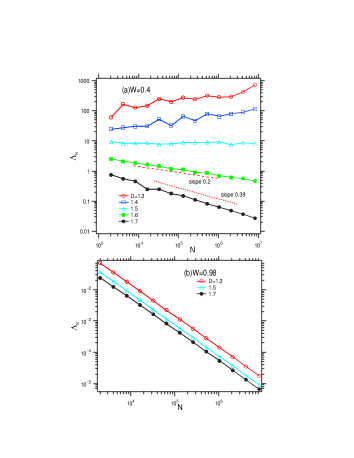
Figure 4: (Color online) The normalized localization length $\Lambda_{N}$ as a function of the system size $N$ with several values of the fractal dimension for the potential strength, (a)$W=0.4$ and (b)$W=0.98$. Note that the data plotted in double-logarithmic scale.

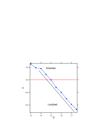
Figure 5: (Color online) The index $\delta$ of Eq.(9) as a function of the fractal dimension $D$ for the case $W=0.4$ in Fig.4. The result has been obtained by the least square fit for the $N-$dependence of the normalized localization length $\Lambda_{N}$. The straight line with a slope $-1.88$ is shown as a guide for eye.

3.3 Strong disorder regime

We examine the $\Lambda_{N}$ behavior to get the delocalization in the relatively strong disorder regime ($W>0.7$).

Figure 4(b) shows the system size dependence of the NLL for $W=0.98$. It clearly shows that the wavefunction goes to localized states in the thermodynamic limit as $\Lambda_{N}\sim N^{-1}$ irrespective of the fractal dimension for the relatively large disorder strength $W=0.98$. Surely we have to investigate the smaller values of $D(\sim 1)$ to make the delocalized states for $W=0.98$ although it is very hard.

Figure 6 illustrates the more detailed behavior of $\Lambda_{N}$ as a function of $D$ and $W$ for $D<3/2$ and the relatively strong disorder $W>0.7$. It is found that the crossing points gradually shift and converge to certain value in the thermodynamic limit $N\to\infty$. This result suggests that the critical value of $D$ decreases less than $3/2$ for the relatively large potential strength $W$.

The $N-$dependence of the NLL for Fig.6(a) and (d) are drawn in Fig.7(a) and (c). The latter both reveal a clear change from the decreasing function to increasing one, as the $D$ and $W$ decreases, respectively. Next, we try to construct the scaling function by the parallel shift of the horizontal axis. If the OPST around the LDT exists, then the NLL behaviors as

$$\Lambda_{N}=f(N/\xi),$$ (11)

where $f(...)$ is the scaling function and $\xi$ is the amount of the parallel shift, corresponding to the localization length or correlation length. In Fig.7(b) and (d), we show the result for the latter shift in the Fig.7(a) and (c), respectively. The general forms of the graph are similar to the results for 1DDS with FFM-potential shima04 .

The upper (lower) brunches are delocalized (localized) regimes. As seen in Fig.7(b) and (d), it seems that the data of the lower branches look like being on a common curve while the data for the upper branches do not belong to an universal curve, as far as present data show. The $N-$dependence of $\Lambda_{N}$ with adequate numerical accuracy for the larger system size is necessary to perform the finite-size scaling analysis around the critical point.

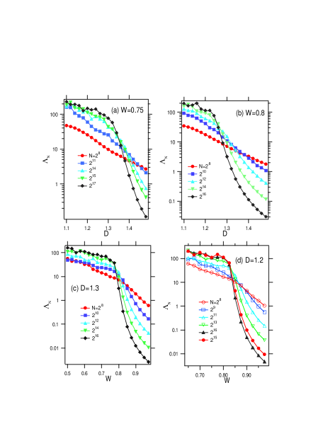
Figure 6: (Color online) Some enlargements of the $D-$dependence and $W-$dependence of the normalized localization length $\Lambda_{N}$. (a)$W=0.75$ and (b)$W=0.8$, (c)$D=1.2$, (d)$D=1.3$. The system size $N$ is varied as $2^{8}$ $\sim 2^{17}$. The averaging is taken over $2^{12}$ realizations. Note that the data are plotted in the semi-logarithmic scale.

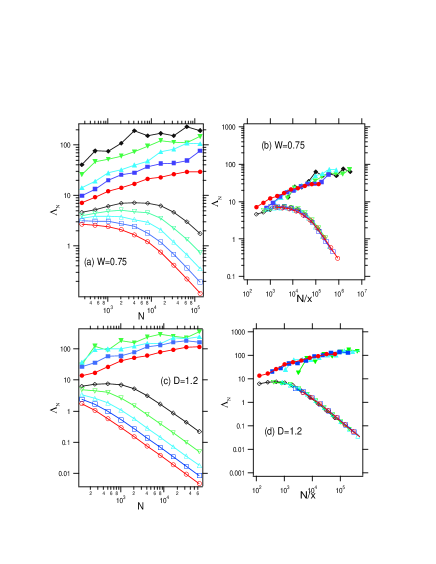
Figure 7: (Color online) The normalized localization length $\Lambda_{N}$ as a function of the system size $N$ with (a)$W=0.75$ for the different values of $D$. $\Lambda_{N}$ as a function of the system size $N$ with (c)$D=1.2$ for the values of $W$. Panels (b) and (d) are the scaling function construction from the numerical data in panels (a) and (c), respectively. Note that all are plotted in double-logarithmic scales.

3.4 phase diagram

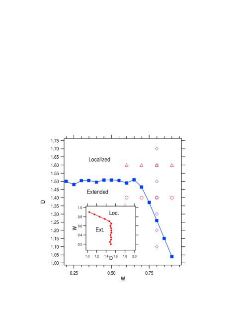
Figure 8: (Color online) Phase diagram of the localization-delocalization transition in the $W-D$ plane. The transition points (denoted by the filled blue squares) have been obtained by numerical plots of the normalized localization length as shown in Fig.2, Fig.3 and Fig.6. The inset shows the diagram in the $D-W$ plane. The open symbols (circles, triangles, rhombuses) indicate the parameter sets used in the quantum diffusion in Fig.9 and Fig.10.

We determined the critical values of $D$ and/or $W$ by the $D-$dependence and $W-$dependence of NLL as seen in Fig.2, Fig.3,

Fig.4 andFig.6. Figure 8 shows the phase diagram in the $D-W$ space separating the localized and delocalized states. The most interesting point here is that the critical disorder strength $W_{c}$ depends on $D$ in the strong disorder regime ($W>0.7$). This result implies that the LDT with the $D-$dependent critical disorder strength is different from the one observed in the 1DDS with FFM-potential, in which it is $W_{c}=2$ in our notation independent of the spectrum exponent $\alpha$ shima04 . And our result in part coincides with one for the FFM-system by Kaya that the critical values of $W$ increases when $\alpha$ increases, while the critical exponent $\nu$ decreases when $\alpha$ increases kaya07 . Accordingly this result suggests that the phase diagram in the $\alpha-W$ space might be different even if the potential sequences are characterized by the same exponent $\alpha$ of the power spectrum in the LDT in the 1DDS.

4 Quantum diffusion

It can be expected that for sufficiently differentiable potentials a band of delocalized states occurs due to destruction of the interference effects in the reflected components of the wavepacket.

In this section, we examine the quantum diffusion of the initially localized wave packet by changing the parameter $D$. We monitor the mean square displacement (MSD) of the wavepacket,

$$m_{2}(t)=\sum_{n}(n-n_{0})^{2}|u(n,t)|^{2},$$ (12)

where $n_{0}$ is an initially localized site. The quantum time-evolution is given by,

$$i\hbar\frac{\partial u(n,t)}{\partial t}=u(n+1,t)+u(n-1,t)+WV(n)u(n,t),$$ (13)

where $n=1,2,...,N$ with initial state $u(n,t=0)=\delta_{n,n_{0}}$ and $\hbar=1$.

Figure 9 shows the time-dependence of the MSD for a fixed potential strength $W=0.8$ and varying the fractal dimension $D$. The parameter sets we used are denoted in Fig.8 by some open symbols. Apparently, the $m_{2}$ ballistically grows for the relatively small values of $D$, and it is localized for the cases with $D>3/2$.

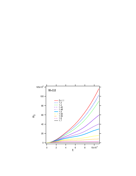
Figure 9: (Color online) The second moment $m_{2}$ as a function of time for some fractal dimensions with $W=0.8$. The bold curve corresponds to the critical case $D=3/2$. We set $\hbar=1$ and $\delta t=0.05$. The system size and sample sizes are $N=2^{16}$ and $10$, respectively.

Next, Fig.10 shows the diffusive properties for some values of the potential strength with fractal dimension, $D=1.4$, $D=1.6$, denoted by the open symbols in Fig.8. It follows that the ballistic-like motion ($m_{2}\sim t^{\beta},\beta>1$) can be obtained for all cases with $D=1.4$, while it is well-localized for the relatively larger value of $W$ in the cases with $D=1.6$. The all of the cases of $D=1.6$ are localized for the long-time calculation. (It is not shown here.)

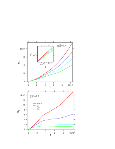
Figure 10: (Color online) The second moment $m_{2}$ as a function of time for some values of $W$ ($W=0.6,0.7,0.8,0.9$) at (a)$D=1.6$ and (b)$D=1.4$. We set $\hbar=1$ and $\delta t=0.05$. The system size and sample sizes are $N=2^{16}$ and $10$, respectively. The inset shows the log-log plots.

As a result, it seems that in the quantum diffusion the critical value $D_{c}$ also around $D\sim 3/2$ which is consistent with the result by the normalized localization length $\Lambda_{N}$ in the last section. However, clear subdiffusive behavior have not been observed around the critical point $D_{c}=3/2$, which is different from the localization-delocalization transition in three-dimensional disordered systems and polychromatically perturbed 1DDS, in which cases an asymptotic behavior, $m_{2}\sim t^{2/3}$, has been obtained at the critical point yamada99 ; yamada04 ; delande08 . This discrepancy is not so surprising if the correlation-induced LDT deviates from the standard OPST as shown in the previous section.

5 Summary and Discussion

In this work we numerically investigated the combined effects of the disorder strength $W$ and the order of the long-range correlation characterized by fractal dimension $D$ in the one-dimensional tight-binding model with the Weierstrass potential. The result based on the normalized localization length strongly suggests that quantum states are localized for $D>3/2$, whereas we have obtained critical disorder strength $W_{c}$ which separates extended and localized regimes for $D\leq 3/2$. In particular, the result that the critical value $D_{c}=3/2$ is not depend on the $W$ is consistent with the result given by Garcia and Cuevas in the weak disorder limit. While the critical value of the fractal dimension depends on the potential strength in the strong disorder regime. Furthermore, the localization-delocalization property reflected on the quantum diffusion of the initially delocalized wavepacket although the subdiffusion could not be observed at the critical case. The disorder strength dependence of the correlation-induced transition is one of the interesting features in the localization-delocalization transition.

Concerning the power spectrum $S(f)\sim 1/f^{\alpha},\alpha=2$, the localization-delocalization transition point $D_{c}=3/2$ is consistent with one predicted in the system with some other correlated potential such as FFM potential izrailev99 ; esmailpour07 ; pinto04 ; croy11 ; petersen12 . Moreover, there are the other types of long-range correlated potential with discrete values such as binary and ternary sequences pinto04 ; yamada91 . One of the common points between the discrete and continuous models is nonstationary of the potential sequences caused by the long-range correlation. Accordingly, the indifferentiable everywhere condition may be unified into the nonstationary condition ($\alpha\geq 2$) for the delocalization in the 1DDS.

An interesting question to ask is whether it is possible to characterize the correlation-induced localization-delocalization transition by the standard one-parameter scaling theory. The study of the finite-size scaling and critical exponents with adequate numerical accuracy are future challenge.

Appendix A Correlation function

The normalized autocorrelation function $C(a,n,m)$ of the Weierstrass potential sequence $V(n)$ can be analytically calculated, as given for the FFM-potential by Petersen and Sandler petersen13 . The explicit form becomes,

$$C(a,n,m) = \frac{<V(n)V(m)>}{<V(n)^{2}>},$$ (14)

$$= \frac{\displaystyle{\sum_{k=0}^{L/2}}a^{-2(2-D)k}\cos\left[2\pi a^{k}\frac{|n-m|}{L}\right]}{\displaystyle{\sum_{k=0}^{L/2}}a^{-2(2-D)k}},$$ (15)

where $<...>$ denotes the ensemble average over the independent phases $\{\phi_{k}\}$ in Eq.(2). We set the distance between positions $\ell\equiv n-m$, and impose the periodic boundary conditions on the correlation function defined in $\ell\in[0,L/2]$. In addition, we set $r=2\ell/L$ and $r\in[0,1]$ for the thermodynamic limit $L\to\infty$. Then the autocorrelation function can be written as

$$C(a,r) = \frac{\displaystyle{\sum_{k=0}^{\infty}}a^{-2(2-D)k}\cos(\pi a^{k}r)}{\displaystyle{\sum_{k=0}^{\infty}}a^{-2(2-D)k}},$$ (16)

In the critical case, $D=3/2$, it becomes

$$C(a,r) = \frac{\displaystyle{\sum_{k=0}^{\infty}}a^{-k}\cos(\pi a^{k}r)}{\displaystyle{\sum_{k=0}^{\infty}}a^{-k}}.$$ (17)

Figure 11 shows the autocorrelation function $C(a=2,r)$ given by Eq.(16) for various values of some fractal dimensions. It follows that the correlation function rapidly decays with complex fluctuation for $D=1.9$. Moreover, the correlation function becomes concave for $D<3/2$ and it linearly decreases near $r\simeq 0$ for the critical value $D_{c}=3/2$. The smaller the fractal dimension $D$ becomes, the correlation becomes more negative. The inset of the Fig. 11 shows the values of the correlation function at $r=1$ as a function of the fractal dimension. It is noted that the correlation function goes negative value at the thermodynamic limit $r=1$ for $D<3/2$. Such a property has been pointed out by Petersen and Sandler in the case of the FFM-potential petersen13 .

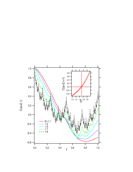
Figure 11: (Color online) The autocorrelation function $C(r)$ as a function of the distance $r$ for various fractal dimension $D$ given by Eq.(16). The parameters are $a=2$, $N=2^{15}$. The inset shows the correlation function between the two most distant points.

References

- (1) K. Ishii, Prog. Theor. Phys. Suppl. 53, 77(1973).
- (2) See, for example, L.M. Lifshiz, S.A. Gredeskul and L.A. Pastur, Introduction to the theory of Disordered Systems, (Wiley, New York,1988).
- (3) P.Stollmann, Caught by Disorder: Bound States in Random Media, (Birkhauser, 2001).
- (4) Ya. Goldsheid, S. Molchanov, and L. Pastur, Funct. Anal. Appl. 11, 1-10 (1977).
- (5) S. Kotani, ”Lyaponov indices determine absolutely continuous spectra of stationary random onedimensional Schrodinger operators”, Proc. Kyoto Stoch. Conf., 1982.
- (6) B. Simon, Commun. Math. Phys. 89, 227-234(1983).
- (7) S. Kotani, Contemp. Math., 50 (1986).
- (8) D. Damanik and R. Killip, Acta Math. 193, 31-72 (2004).
- (9) F.A.B.F.de Moura, and M.L.Lyra, Phys. Rev. Lett. 81 3735(1998).
- (10) F.M.Izrailev and A.A.Krokhin, Phys. Rev. Lett. 82, 4062(1999).
- (11) L.Y. Gong, P.Q. Tong, and Z.C. Zhou, Eur. Phys. J. B 77, 413-417(2010).
- (12) Chao-Sheng Deng, and HuiXu, Physica E 44 1473-1477(2012).
- (13) T. Kaya, Eur. Phys. J. B 55 (2007) 49.
- (14) Longyan Gong, Ling Wei, Shengmei Zhao, and Weiwen Cheng, Phys. Rev. E 86, 061122 (2012).
- (15) C. Albrecht and S. Wimberger, Phys. Rev. B 85, 045107 (2012).
- (16) S. Bocker, W. Kirsch, and P. Stollmann, ”Spectral Theory for Nonstationary Random Potentials”, Interacting Stochastic Systems 2005, pp 103-117 Lecture Notes in Mathematics.
- (17) C.R. de Oliveira and G.Q. Pellegrino, J. Phys. A 34, L239-L243 (2001).
- (18) H.Shima, T.Nomura and T.Nakayama, Phys. Rev. B 70, 075116(2004).
- (19) N. P. Greis and H. S. Greenside, Phys. Rev. A 44, 2324(1991).
- (20) A. M. Garcia-Garcia, and E. Cuevas, Phys. Rev. B 79, 073104 (2009).
- (21) A. M. Garcia-Garcia, and E. Cuevas, Phys. Rev. B 82, 033412 (2010).
- (22) A. E. B. Costa and F. A. B. F. DE Moura, Int. J. Mod. Phys. C 22, 573 (2011).
- (23) G.M. Petersen and N. Sandler, Phys. Rev. B 87,195443(2013).
- (24) E. Abrahams, P. W. Anderson, D. C. Licciardello, and T. V. Ramakrishnan, Rhys. Rev.Lett. 42, 673 (1979).
- (25) H.Yamada and K.S. Ikeda, Phys. Rev. E 59, 5214-5230(1999).
- (26) H.Yamada and K.S.Ikeda, Phys. Lett. A 328, 170-176(2004).
- (27) J. Chabe, G. Lemarie, B. Gremaud, D. Delande, P. Szriftgiser, Phys. Rev. Lett. 101, 255702(2008).
- (28) A. Esmailpour, H. Cheraghchi, P. Carpena and M. R. R. Tabar, J. Stat. Mech. P09014(2007).
- (29) R. A. Pinto, M. Rodriguez,1 J. A. Gonzalez, and E. Medina, Phys. Lett. A 341, 101-106(2005).
- (30) A. Croy, P. Cain, and M. Schreiber, Eur. Phys. J. B 82, 20212 (2011).
- (31) G.M. Petersen and N. Sandler, arXiv:1206.3370v3 [cond-mat.dis-nn].
- (32) H. Yamada, M. Goda and Y. Aizawa, J. Phys.: Condens. Matter 3, 10043(1991), H.Yamada, Phys. Rev. B 69 014205(2004), H.Yamada, Phys. Lett. A 325 118(2004), H. Yamada, Phys. Lett. A 332, 65-73(2004), H.Yamada and T.Okabe, Phys. Rev. E 63, 026203(2001).