A quasi-linear analysis of the impurity effect on turbulent momentum transport and residual stress

Abstract

We study the impact of impurities on turbulence driven intrinsic rotation (via residual stress) in the context of the quasi-linear theory. A two-fluid formulation for main and impurity ions is employed to study ion temperature gradient modes in sheared slab geometry modified by the presence of impurities. An effective form of the parallel Reynolds stress is derived in the center of mass frame of a coupled main ion-impurity system. Analyses show that the contents and the radial profile of impurities have a strong influence on the residual stress. In particular, an impurity profile aligned with that of main ions is shown to cause a considerable reduction of the residual stress, which may lead to the reduction of turbulence driven intrinsic rotation.

I Introduction

The presence of a certain amount of impurities is, in some sense, an inevitable consequence of tokamak plasma operation. The contents and the radial profile of the dominant impurity species depend on the details of discharge conditions, plasma-wall interaction, and the physical process of impurity transport. In tokamaks, the material constituting plasma facing components (PFCs), for instance, carbon in DIII-DDIIID and KSTARKSTAR , or tungsten in ASDEX-UAUG , JETJET and ITERITER_impW , is usually observed as a dominant impurity species. In addition to impurities originating from the surrounding PFCs, a considerable amount of helium ash will be present in ITER or fusion reactors as a result of fusion reactionITER_impHe ; Polevoi .

Studies of impurity transport in tokamaks have usually focused on the determination of impurity profiles (e.g. the impurity peaking factor) from either neoclassicalHirsh-Sig ; NeoKim ; Neo2 or turbulent mechanismsGarbet ; AP . The main goal of this endeavour is to predict the degree of impurity accumulation for a given set of discharge parameters to avoid deleterious effect from impurity accumulation. Turbulent transport of impurities, which has been a subject of an extensive study in fusion plasma physics for decades Garbet ; AP ; Coppi ; Dong1 ; Dong2 ; Dong ; FW is rekindling interest in this regard since recent experimental evidence has shown the importance of the turbulent transport process in determining the core impurity profileAngioni-JET .

When impurity concentration is sufficiently low, one may treat the impurities as passive reactants to background turbulence. In this case, the so-called trace approximation has been used to study turbulent impurity transportAP ; Nordman . If impurity concentration is considerable, however, they start to affect microinstabilityCoppi ; Dong1 ; Dong2 ; Dong and the trace approximation becomes invalid, as pointed out by Fülöp and NordmanFN . Most notably, the alignment of a impurity profile with that of main ions has been known to yield a significant change of stability of the ion temperature gradient (ITG) mode, sometimes leading to the destabilization of an independent impurity drift modeTang ; Dong

Our interest in this paper lies in the study of the impact of impurities on turbulent momentum transport, in particular, the generation of intrinsic rotation via residual stressRS1 ; RS2 . We note that few results are available in this aspect, given a lot of published papers on turbulent impurity transport in tokamaks. Intrinsic rotation in magnetic fusion plasmas is thought to be generated through the conversion of radial inhomogeneity into $\left<k_{||}\right>$ (= spectrally averaged wavenumber in parallel direction) asymmetry via residual stress. This conversion process requires some symmetry breaking mechanismGurcan1 ; Gurcan2 ; McDevitt ; Singh ; Ram . An early paper calculated the particle flux in the presence of combined ITG, impurity and parallel velocity gradients, but not addressed the turbulent residual stress giving rise to intrinsic rotationDong .

The purpose of this study is to provide a simple physics insight into which how turbulence driven residual stress is related to the characteristics of impurities. Intuitively, one may expect that the change of stability and characteristics of an unstable mode structure in the presence of a considerable amount of impurities will alter the turbulent residual stress. This effect may change the amount of intrinsic torque anticipated in toakamak experiments. Since intrinsic rotation is envisioned to provide necessary plasma rotation in reactor-relevant tokamak experiments, including ITER, because of the limited capability of driving the necessary torque in a reactor by neutral beam injection, it is of importance to conduct a sufficiently detailed study of this effect.

To address the problem mentioned above, we employ a set two fluid equations for main and impurity ions. By treating impurities as a separate species satisfying impurity fluid equations, we can incorporate the effects of impurities on the characteristics of the ITG mode self-consistently. For simplicity, we adopt the sheared slab geometry. By avoiding the complication in analysis due to the sophisticated toroidal geometry, we focus on the basic physics of the impurity effect on residual stress in the presence of impurity-modified ITG turbulence. Analyses show that the relative importance of residual stress to the diffusive momentum flux is reduced when the gradient of impurity and main ions has the same sign. This indicates a possible decrease of intrinsic rotation when a considerable amount of core-peaked impurity is present.

The remainder of the paper is organized as follows. In Sec. II, we describe the basic formulation. A derivation is given of a linear dispersion relation and an eigenmode equation for ITG modes using two fluid equations for ions and impurities. In Sec. III, we perform a numerical analysis to evaluate eigenmode structures of unstable modes. A detailed study of the change of eigenmode characteristics, such as the variation of the mode shift off the rational surface, is made in this section. Section IV is devoted to the quasi-linear calculations of momentum flux. After introducing some underlying assumptions made in this study, we calculate turbulent parallel Reynolds stress (both diffusive and residual stresses) in the context of the quasi-linear analysis. A particular emphasis is placed on the evaluation of the ratio of residual stress to diffusive one, which ameliorates the limitation of the quasi-linear theory. Possible implications of the results will be discussed in this section. We conclude this paper in Sec. V with a brief summary of main results and some discussions.

II Formulation

We begin with a set of two fluid equations for main and impurity ions consisting of the conservation of density ($n_{j}$), parallel momentum density $(m_{j}n_{j}v_{\parallel j})$, and pressure $P_{j}$,

$$\frac{\partial n_{j}}{\partial t}+\nabla\cdot(n_{j}{\mathbf{v}}_{j})=0,$$

$$m_{j}n_{j}\frac{d{\mathbf{v}}_{\parallel j}}{dt}+\nabla_{\parallel}P_{j}+n_{j}e_{j}\nabla_{\parallel}\phi=0,$$

$$\frac{dP_{j}}{dt}+\Gamma P_{j}\nabla\cdot{\mathbf{v}}_{\parallel}=0,$$ (1)

where the subscript $j=i$ ($Z$) denotes the main (impurity) ions, $\phi$ is the electrostatic potential fluctuation, and $\Gamma$ is the adiabatic index. The fluid velocity is decomposed into the parallel and the perpendicular components, $\mathbf{v}_{j}=\mathbf{v}_{\parallel j}+\mathbf{v}_{\perp j}$ with $\mathbf{v}_{\perp j}=\mathbf{v}_{Ej}+\mathbf{v}_{*j}+\mathbf{v}_{pj}$, where $\mathbf{v}_{Ej}$, $\mathbf{v}_{*j}$, and $\mathbf{v}_{pj}$ are the $E\times B$, the diamagnetic, and the polarization drift of the species $j$, respectively. We employ the sheared slab geometry with a background magnetic field in the vicinity of a reference surface ($r_{0}$), $\vec{B}_{0}=B_{0}\left(\hat{z}+{x}/{L_{s}}\hat{y}\right)$. Here, $L_{s}=qR/rq^{\prime}$ is the magnetic shear scale length with $q$ the safety factor, $R$ ($r$) the major (minor) radius, and the prime denotes a derivative with respect to $x=r-r_{0}$.

Linearization of Eq. (1) can be done straightforwardly giving rise to

$$d_{t}^{E}(n_{i}-\nabla^{2}_{\perp}\phi)+L_{ei}(1+K_{i}\nabla^{2}_{\perp})\nabla_{y}\phi+\nabla_{\parallel}v_{\parallel i}=0,$$ (2a)

$$d_{t}^{E}v_{\parallel i}-\hat{V}_{0\parallel i}^{\prime}\nabla_{y}\phi+\nabla_{\parallel}\phi+\tau_{i}\nabla_{\parallel}p_{i}=0,$$ (2b)

$$d_{t}^{E}p_{i}+L_{ei}(1+\eta_{i})\nabla_{y}\phi+\Gamma\nabla_{\parallel}v_{\parallel i}=0,$$ (2c)

$$d_{t}^{E}(n_{Z}-\frac{\mu}{Z}\nabla^{2}_{\perp}\phi)+L_{eZ}(1+\frac{\mu}{Z^{2}}K_{Z}\nabla^{2}_{\perp})\nabla_{y}\phi+\nabla_{\parallel}v_{\parallel Z}=0,$$ (2d)

$$d_{t}^{E}v_{\parallel Z}-\hat{V}_{0\parallel Z}^{\prime}\nabla_{y}\phi+\frac{Z}{\mu}\nabla_{\parallel}\phi+\frac{\tau_{Z}}{\mu}\nabla_{\parallel}p_{Z}=0,$$ (2e)

$$d_{t}^{E}p_{Z}+L_{eZ}(1+\eta_{Z})\nabla_{y}\phi+\Gamma\nabla_{\parallel}v_{\parallel Z}=0,$$ (2f)

where $d_{t}^{E}=(\partial_{t}+x\hat{V}_{E0}^{\prime}\nabla_{y})$ with $\hat{V}_{E0}^{\prime}$ the normalized equilibrium $E\times B$ flow shear. Various quantities in Eq. (2) are normalized as $x=x/\rho_{s}$, $y=y/\rho_{s}$, $z=z/L_{ne}$, $t=t/(L_{n_{e}}/c_{s})$, $\phi=(e\phi/T_{e})(L_{n_{e}}/\rho_{s})$, $n_{i}=(n_{i1}/n_{i0})(L_{n_{e}}/\rho_{s})$, $n_{Z}=(n_{Z1}/n_{Z0})(L_{n_{e}}/\rho_{s})$, $v_{i||}=(v_{i\parallel 1}/c_{s})(L_{n_{e}}/\rho_{s})$, $v_{Z||}=(v_{Z\parallel 1}/c_{s})(L_{n_{e}}/\rho_{s})$, $\hat{V}_{E0}^{\prime}=(L_{n_{e}}/c_{s})(dV_{E0}/dx)$, $\hat{V}_{0\parallel i}^{\prime}=(L_{n_{e}}/c_{s})(dV_{i0\parallel}/dr)$, $\hat{V}_{0\parallel Z}^{\prime}=(L_{n_{e}}/c_{s})(dV_{Z0\parallel}/dr)$, $p_{i}=(P_{i1}/P_{i0})(L_{n_{e}}/\rho_{s})$, $p_{Z}=(P_{Z1}/P_{Z0})(L_{n_{e}}/\rho_{s})$ with $L_{ne}^{-1}=-\nabla n_{0}/n_{0}$ the equilibrium density scale length, $c_{s}=\sqrt{T_{e0}/m_{i}}$ ($T_{e0}$: equilibrium electron temperature), and $\rho_{s}=c_{s}/\Omega_{i}$ the ion-acoustic Larmor radius. Also, various dimensionless parameters are defined as $\mu=m_{Z}/m_{i}$, $\eta_{i}={L_{n}}/{L_{Ti}}$ with $L_{Ti}^{-1}=-\nabla T_{0i}/T_{0i}$ the equilibrium ion temperature scale length, $\eta_{Z}=L_{nZ}/L_{TZ}$, $K_{i}=\tau_{i}(1+\eta_{i})$ with $\tau_{i}=T_{i0}/T_{e0}$, $K_{Z}=\tau_{Z}(1+\eta_{Z})$ with $\tau_{Z}=T_{Z0}/T_{e0}$, $L_{ei}=L_{n_{e}}/L_{n_{i}}$, and $L_{eZ}=L_{n_{e}}/L_{n_{Z}}$.

We consider perturbations of the form $f=f_{k}(x)\exp\left(ik_{y}y+ik_{z}z-i\omega t\right)$, where $\omega$ is normalized to $c_{s}/L_{n}$. Then, one can calculate ion and impurity density fluctuations from Eqs. (2a) to (2f),

$$n_{ik}=-\frac{1}{\hat{\omega}}\left[\left(\hat{\omega}+k_{y}L_{ei}K_{i}\right)k_{\perp}^{2}-k_{y}L_{ei}-\frac{k_{\parallel}\hat{\omega}}{\hat{\omega}^{2}-k_{\parallel}^{2}\tau_{i}\Gamma}\left({k_{\parallel}-k_{y}\hat{V}_{0\parallel i}^{\prime}}+\frac{k_{y}k_{\parallel}L_{ei}K_{i}}{\hat{\omega}}\right)\right]\phi_{k},$$

and

$$n_{Zk}=-\frac{1}{\hat{\omega}}\left[\frac{\mu}{Z}\left(\hat{\omega}+\frac{k_{y}L_{eZ}K_{Z}}{Z}\right)k_{\perp}^{2}-{k_{y}L_{eZ}}-\frac{k_{\parallel}\hat{\omega}}{\hat{\omega}^{2}-k_{\parallel}^{2}({\tau_{Z}}/{\mu})\Gamma}\left({k_{\parallel}-k_{y}\hat{V}_{0\parallel Z}^{\prime}}+\frac{k_{y}k_{\parallel}L_{eZ}K_{Z}}{\hat{\omega}}\right)\right]\phi_{k},$$

where $\hat{\omega}=\omega-k_{y}x\hat{V}_{E0}^{\prime}$ is the normalized frequency of the fluctuation accounting for the Doppler shift.

Ions, impurities, and electrons are coupled through the quasi-neutrality condition, $n_{ek}=(1-f_{Z})n_{ik}+f_{Z}n_{Zk}$ where $f_{Z}={Zn_{Z0}}/{n_{e0}}$ is the fraction of impurity under consideration. Assuming the adiabatic electron response, $n_{ek}=\phi_{k}$, one can derive, after a little algebra, an eigenvalue equation in $\phi_{k}$,

$$\frac{d^{2}\phi_{k}}{dx^{2}}+U(k_{\parallel},k_{y},\hat{\omega})\phi_{k}=0,$$ (3)

where

$$U(k_{\parallel},k_{y},\hat{\omega}) = -k_{y}^{2}+\frac{k_{y}-\hat{\omega}}{\alpha\hat{\omega}+k_{y}A}+\frac{(1-f_{Z})\hat{\omega}}{(\alpha\hat{\omega}+k_{y}A)(\hat{\omega}^{2}-\tau_{i}k_{\parallel}^{2}\Gamma)}\left(k_{\parallel}^{2}-k_{y}k_{\parallel}\hat{V}_{0\parallel i}^{\prime}+\frac{k_{y}k_{\parallel}^{2}L_{ei}K_{i}}{\hat{\omega}}\right)$$ (4)

$$+\frac{f_{Z}\hat{\omega}}{(\alpha\hat{\omega}+k_{y}A)\left[\hat{\omega}^{2}-({\tau_{Z}}/{\mu})k_{\parallel}^{2}\Gamma\right]}\left(\frac{Z}{\mu}k_{\parallel}^{2}-k_{y}k_{\parallel}\hat{V}_{0\parallel Z}^{\prime}+\frac{k_{y}k_{\parallel}^{2}L_{eZ}K_{Z}}{\mu\hat{\omega}}\right)$$

with the definitions $\alpha=1-f_{Z}+({\mu}/{Z})f_{Z}$ and $A=(1-f_{Z})L_{ei}K_{i}+f_{Z}({\mu}/{Z^{2}})L_{eZ}K_{Z}$. Equation (4) represents a complete potential function for the ITG eigenmode modified by the presence of impurities whose fraction is $f_{Z}$. Following Singh et. al.,Ram , we assume that the mode frequency is much higher than the equilibrium shearing rate and the ion acoustic wave frequency, i.e., $\omega^{2}\gg k_{\parallel}^{2}\tau_{i}\Gamma$ and $\omega\gg k_{y}\hat{V}_{E0}^{\prime}$. We further assume that the equilibrium ion and impurity velocity profiles are equal, $\hat{V}_{0\parallel i}=\hat{V}_{0\parallel Z}=\hat{V}_{0\parallel}$. Under these assumptions, Eq. (4) is reduced to

$$U(k_{y},\omega,x)=A_{0}+A_{1}x+A_{2}x^{2},$$ (5)

where

$$A_{0}=-k_{y}^{2}+\frac{k_{y}-\omega}{\alpha\omega+k_{y}A},$$

$$A_{1}=\frac{k_{y}}{\alpha\omega+k_{y}A}\left(\hat{V}_{E0}^{\prime}-\frac{k_{y}s}{\omega}\hat{V}_{\parallel i}^{\prime}\right),$$

$$A_{2}=\frac{\beta\omega+k_{y}B}{\alpha\omega+k_{y}A}\frac{k_{y}^{2}s^{2}}{\omega^{2}},$$

with the definitions $\beta=1-f_{Z}+({Z}/{\mu})f_{Z}$ and $B=(1-f_{Z})L_{ei}K_{i}+({f_{Z}}/{\mu})L_{eZ}K_{Z}$. Equation (5) with the coefficients $A_{0},A_{1},A_{2}$ is a simplified form of the impurity-modified potential function for the ITG mode with the frequency $\hat{\omega}$ and the mode number $k_{y}$. The impurity effect on mode characteristics are now contained in the parameters $\alpha$, $A$ and $B$ in this formulation.

Solutions to Eq. (3) are well-known Hermite polynomials. To make an analytical progress, we consider the most dominant zeroth order Hermite polynomial. Then, the eigenfunction becomes

$$\phi_{k_{y}} =\phi_{0}\exp\left[-\frac{1}{2}i\sqrt{A_{3}}\left(x+\frac{A_{2}}{A_{3}}\right)^{2}\right]$$ (6)

$$=\Phi_{0k_{y}}\exp\left[-\frac{1}{2}\left(\frac{x-X_{0}}{\Delta_{k_{y}}}\right)^{2}\right],$$

where

$$X_{0}=-\left(Re\frac{A_{2}}{2A_{3}}+\frac{Re\sqrt{A_{3}}}{Im\sqrt{A_{3}}}Im\frac{A_{2}}{2A_{3}}\right)$$ (7)

is the shift of the mode from the mode rational surface,

$$\Delta^{-2}_{k_{y}}=-Im\sqrt{A_{3}}$$ (8)

is the width of the mode, and

$$\Phi_{0k_{y}} =\Phi_{0}(A_{1},A_{2},A_{3})\exp\left[-\frac{i}{2}Re\sqrt{A_{3}}\left(x+Re\frac{A_{2}}{2A_{3}}-\frac{Im\sqrt{A_{3}}}{Re\sqrt{A_{3}}}Im\frac{A_{2}}{2A_{3}}\right)^{2}\right].$$ (9)

We plug Eq. (6) into Eq. (3) and evaluate the resulting relation,

$$\left(A_{1}-\frac{A_{2}^{2}}{4A_{3}}\right)/\sqrt{-A_{3}}=1,$$

which converts into the following dispersion relation,

$$-k_{y}^{2}+\frac{k_{y}-\omega}{\alpha\omega+k_{y}A}-\frac{k_{y}^{2}}{4D(\alpha\omega+k_{y}A)^{2}}\left(\frac{\omega}{k_{y}s}\hat{V}_{E0}^{\prime}-\hat{V}_{0\parallel}^{\prime}\right)^{2}=i\sqrt{D}\frac{k_{y}s}{\omega},$$ (10)

where $D=(\beta\omega+k_{y}B)/(\alpha\omega+k_{y}A)$. One can rearrange Eq. (10) to obtain

$$\omega^{2}(1+\alpha k_{y}^{2})+k_{y}\omega(-1+k_{y}^{2}A+i\sqrt{D}s\alpha)+i\sqrt{D}k_{y}^{2}sA=-\frac{k_{y}^{2}\omega}{4D(\alpha\omega+k_{y}A)}\left(\frac{\omega}{k_{y}s}\hat{V}_{E0}^{\prime}-\hat{V}_{0\parallel}^{\prime}\right)^{2}.$$ (11)

It is an easy task to show that Eq. (11) recovers the dispersion relation without impuritiesSingh when $f_{Z}=0$, $\alpha=1$, $A=K_{i}$ and $D=1$.

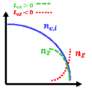
Figure 1: A schematic diagram illustrating the wall-peaked ($L_{eZ}<0$, red dotted) and the core-peaked ($L_{eZ}>0$, green dashed) impurity profiles. Solid blue line represents an equilibrium plasma density profile.

Equation (11) is the desired equation to be analysed in this paper. It has been known that the radial profile of an impurity has a significant influence on ITG stabilityCoppi ; Tang ; Dong1 ; Dong2 . In the case of a wall-peaked impurity profile schematically shown in Fig. 1 (red dotted line), the ITG mode is destabilized while the core-peaked one (green dashed line in Fig. 1), stabilizes it. Therefore, before performing a detailed numerical analysis, it is instructive to examine if Eq. (11) recovers these known results. To make the analysis simple, we first consider Eq. (11) in the slow mode (i.e., the long wavelength) limitSingh ; Balescu which is characterized by the relation $|k_{y}^{2}A|\ll 1$. We further assume that $\hat{V}_{E0}^{\prime}=\hat{V}_{0\parallel}^{\prime}=0$, and $s\ll 1$. Then, one obtains a purely growing mode with the growth rate,

$$\omega_{0i}\sim ik_{y}sA =ik_{y}s\left[(1-f_{Z})L_{ei}K_{i}+f_{Z}\frac{\mu}{Z^{2}}L_{eZ}K_{Z}\right]$$ (12)

$$=ik_{y}s\left[K_{i}-f_{Z}L_{eZ}\left(K_{i}-\frac{\mu}{Z^{2}}K_{Z}\right)\right],$$

where the relation $L_{ei}=\left({1-f_{Z}L_{eZ}}\right)/(1-f_{Z})$ is used from the quasi-neutrality condition. From Eq. (12), one can see that the mode becomes stabilized when $L_{eZ}>0$ (i.e., the core-peaked case), while it is destabilized when $L_{eZ}<0$ (i.e., the wall-peaked case). In slab ITG modes, this can be interpreted by an effective reduction or enhancement of negative compressibility due to impurity inertia. We now consider the other limit where the relation $|1-k_{y}^{2}A|\leq s\ll 1$ holds, i.e., the fast mode limit. In this limit, the fastest growing mode occurs at $k_{y}^{2}=A^{-1}$, giving rise to the dispersion relation,

$$\omega=(-1+i)\sqrt{\frac{s}{2(1+\alpha/A)}}.$$

Again, the mode becomes stabilized (destabilized) when $L_{eZ}>0$ ($L_{eZ}<0$) due to the decrease (increase) of $A=(1-f_{Z})L_{ei}K_{i}+(\mu/Z^{2})f_{Z}L_{eZ}K_{Z}$.

III Eigenmode analysis

Figure 2(a) and 2(b) show the real frequency ($\omega_{r}$) and the growth rate ($\gamma$), respectively, as a function of $L_{eZ}=L_{n_{e}}/L_{n_{Z}}$ for two representative impurity ions in tokamaks, ${\rm{He}^{2+}}$ in blue and $\rm{C}^{6+}$ in red. To produce Fig. 2 we solved Eq. (11) numerically using the parameters, $\tau_{i}=\tau_{Z}=1$, $f_{z}=0.3$, $k_{y}=0.5$, $\eta_{i}=2$, $\hat{V}_{E0}^{\prime}=-0.01$, and $\hat{V}_{0\parallel}^{\prime}=-0.1$. The wavenumber $k_{y}=0.5$ corresponds to the most unstable mode giving rise to the maximum growth rate in this case. The equilibrium $E\times B$ shear $\hat{V}_{E0}^{\prime}=-0.01$ roughly corresponds to $E_{r}\approx-5~{}kV$ if we assume $B_{T}=1~{}\rm{Tesla}$ and $T_{e}\approx 3~{}keV$. This is approximately $\sim 1/4$ of the radial electric field well in typical H-mode dischargesEr-DIII ; Er-JET . Deuterium is used as the main ion species in these calculations and throughout the paper. Figure 2 basically confirms the analytic estimation of the impact of $L_{eZ}$ on ITG stability presented in Sec. II: stabilization (destabilization) of the ITG mode by a wall-peaked (core-peaked) impurity profile. The lighter impurity species (${\rm He}^{2+}$) shows a little higher real frequency and growth rate compared to a heavier one, but the deviation is insignificant as long as the $f_{Z}$ value is fixed.

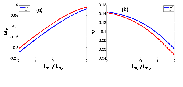
Figure 2: The real frequency ($\omega_{r}$) (a) and the growth rate ($\gamma$) of the most unstable eigenmode corresponding to $k_{y}=0.5$ as a function of the ratio between the equilibrium scale length of the electron ($L_{ne}=-n_{0}/\nabla n_{0}$) to the impurity ($L_{nZ}=-n_{Z0}/\nabla n_{Z0}$) density. $\rm{He}^{2+}$ (blue) and $\rm{C}^{6+}$ (red) are considered as representative impurities in tokamaks. Deuterium is assumed to be the main ion species. Plasma parameters being used are $\tau_{i}=\tau_{Z}=1$, $f_{Z}=0.3$, $\eta_{i}=2$, $\hat{V}_{E0}^{\prime}=-0.01$, and $\hat{V}_{0\parallel}^{\prime}=-0.1$.

The impact of impurity fraction, $f_{Z}$, on the eigenfrequncy is shown in Figs. 3(a) and 3(b). In these figures, we consider two different impurity profiles: $L_{eZ}=1$ (solid) and $L_{eZ}=-1$ (dotted). Other parameters to produce Fig. 3 are same as those of Fig. 2. The stabilization ($L_{eZ}=1$) or destabilization ($L_{eZ}=-1$) of the ITG mode by impurities becomes stronger as $f_{Z}$ increases. An interesting observation is that there is asymmetry in the stabilization and destabilization by impurities for a fixed $f_{Z}$ value, as can be seen in Fig. 3(b). Thus, a heavy impurity with a core-peaked profile has a stronger stabilizing influence compared to the lighter impurity, while the destabilization effect due to it with a wall-peaked profile is weaker than that of the latter.

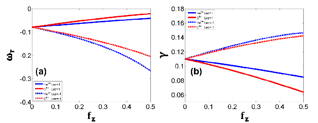
Figure 3: The real frequency ($\omega_{r}$) (a) and the growth rate ($\gamma$) of the most unstable eigenmode as a function of impurity contents ($f_{Z}$). Solid and dotted lines represent when $L_{eZ}=1$ and $-1$, respectively. $\rm{He}^{2+}$ (blue) and $\rm{C}^{6+}$ (green) are considered as representative impurities. The same plasma parameters (except for $f_{Z}$) as those in Fig. 2 have been used.

Of particular interest in this paper is the strength of the mode shift ($X_{0}$) given in Eq. (7). This is because $X_{0}$ driven by the $E\times B$ shear is an essential quantity in the calculation of residual stressGurcan1 ; Gurcan2 ; Singh ; Ram , hence the intrinsic rotation, in the quasi-linear theory. Figure 4(a) shows $|X_{0}|$ vs. $L_{n_{e}}/L_{n_{Z}}$ for $\rm{C}^{6+}$ when $f_{z}=0.1$ (solid) and 0.3 (dotted). In general, $|X_{0}|$ for a given value of $\hat{V}_{E0}^{\prime}$ decreases as the local impurity profile changes from wall- to core-peaked one, regardless of $f_{Z}$. Thus, one may expect that the ITG-driven residual stress will increase as the impurity profile changes from the wall to core-peaked one. The trend of $|X_{0}|$ reduction shows a remarkable difference depending on the impurity contents. When $f_{Z}=0.1$, $|X_{0}|$ shows an almost linear behaviour in the whole range of conceivable $L_{n_{e}}/L_{n_{Z}}$ values, as can be seen in Fig. 4(a). When $f_{Z}=0.3$, however, $|X_{0}|$ does not change much when negative $L_{n_{e}}/L_{n_{Z}}<0$, while it starts to decrease very rapidly as soon as $L_{n_{e}}/L_{n_{Z}}$ becomes positive. For example, the reduction in $|X_{0}|$ as $L_{n_{e}}/L_{n_{Z}}$ changes from $0$ to $1$ is $\sim 25\%$ and $\sim 9\%$ when $f_{Z}=0.3$ and $0.1$, respectively.

Figure 4(b) shows the effect of $f_{Z}$ on $|X_{0}|$ when $L_{n_{e}}/L_{n_{Z}}=1$ (solid) and $-1$ (dotted), respectively. Unlike the growth rate, $|X_{0}|$ always decreases as $f_{Z}$ increases, regardless of the impurity profile shape. The decrease of $X_{0}$ can be seen more clearly in the core-peaked impurity profile which exhibits a significant reduction of $|X_{0}|$ when $f_{Z}$ increases. The impurity effect on $X_{0}$ is not considerable for a wall-peaked profile with a moderate dilution of a plasma, i.e.,, when $f_{Z}<0.2$. A core-peaked profile, however, will result in large reduction of $X_{0}$, which eventually leads to a significant decrease of residual stress. This is a subject for the next section.

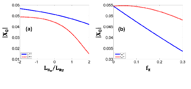
Figure 4: The shift ($X_{0}$) of the most unstable ITG mode ($k_{y}=0.5$) off the rational surface as a function of $L_{eZ}=L_{n_{e}}/L_{n_{Z}}$ (a) and $f_{Z}$ (b). Blue solid and red dotted lines in (a) represent when $f_{Z}=0.1$ and 0.3, respectively. In (b), blue solid and red dotted lines show when $L_{eZ}=1$ and $-1$, respectively. $\rm{C}^{6+}$ impurity is used with plasma parameters $\tau_{i}=\tau_{Z}=1$, $\eta_{i}=2$, $\hat{V}_{E0}^{\prime}=-0.01$, and $\hat{V}_{0\parallel}^{\prime}=-0.1$.

IV Momentum Flux and Residual Stress

In this section, we calculate the parallel Reynolds stress in the presence of a small fraction of impurity ions. To begin, we add parallel force balance equations for ions and impurities, Eqs. (2b) and (2e), respectively, and take an ensemble average of the resulting equation to obtain

$$\frac{\partial\left<V_{\parallel}\right>}{\partial t}=-\frac{\partial}{\partial r}\left[\Pi^{(i)}_{r||}+\frac{m_{Z}n_{Z0}}{m_{i}n_{i0}}\Pi^{Z}_{r||}\right]+\frac{1}{m_{i}n_{i0}}\left[\left<\tilde{n}_{i}\nabla_{\parallel}\tilde{T}_{i}\right>+\left<\tilde{n}_{Z}\nabla_{\parallel}\tilde{T}_{Z}\right]\right>.$$ (13)

In Eq. (13), $\left<A\right>$ represents the ensemble average of a quantity $A$. In this study, we define an effective fluid velocity as $\left<V_{\parallel}\right>=\left<V_{\parallel i}\right>+\left[(m_{Z}n_{Z0})/(m_{i}n_{i0})\right]\left<V_{\parallel Z}\right>$, which is the center of mass (CM) velocity in an equilibrium state of a combined ion-impurity system. $\Pi^{(i)}_{r\parallel}$ and $\Pi^{(Z)}_{r\parallel}$ are the contribution to the total parallel Reynolds stress from main ions and impurities, respectively. The last two terms in Eq. (13) represent the parallel turbulence acceleration whose characteristics have been studied elsewhereWang ; Garbet-TA .

In this study, we do not take the turbulence acceleration effect into account, focusing ourselves on the residual stress due to the symmetry breaking by the $E\times B$ shear. Also, we assume that the equilibrium flow velocities of main ions and impurities under consideration is equal, ${V}_{0\parallel i}={V}_{0\parallel Z}\equiv V_{0||}$. This assumption is strictly valid at the edge region of a tokamak plasma with sufficiently high collisionality. We keep this assumption in this study by taking notice of the validity of our analysis. Then, Eq. (13) is simplified into the form,

$$\frac{\partial\left<V_{\parallel}\right>}{\partial t}=-\nabla_{r}\Pi^{\rm{eff}}_{r\parallel},$$ (14)

where $\Pi^{\rm{eff}}_{r\parallel}$ is the effective parallel Reynolds stress of the coupled ion-impurity system. One can write $\Pi^{\rm{eff}}_{r\parallel}$ in a canonical form in the quasilinar theory,

$$\Pi_{r\parallel}^{\rm eff}=-\chi_{\phi}^{\rm{eff}}\frac{\partial V_{\parallel 0}}{\partial r}+\Pi_{res}^{\rm{eff}}$$ (15)

with $\chi_{\phi}^{\rm{eff}}$ and $\Pi_{res}^{\rm{eff}}$ the effective momentum diffusivity and the residual stress defined at the CM frame, respectively. Then, it is easy to derive expressions for $\chi_{\phi}^{\rm{eff}}$ and $\Pi_{res}^{\rm{eff}}$ to obtain

$$\chi_{\phi}^{\rm{eff}}=\frac{1}{1+\hat{M}}\chi^{i}_{\phi}+\frac{\hat{M}}{1+\hat{M}}\chi^{Z}_{\phi},$$ (16)

$$\Pi_{res}^{\rm{eff}}=\frac{1}{1+\hat{M}}\Pi^{i}_{res}+\frac{\hat{M}}{1+\hat{M}}\Pi^{Z}_{res},$$ (17)

where $\hat{M}=m_{Z}n_{Z0}/m_{i}n_{i0}$, $\chi^{i}_{\phi}$ ($\chi^{Z}_{\phi}$) is the turbulent ion (impurity) momentum diffusivity, and $\Pi^{i}_{res}$ ($\Pi^{Z}_{res}$) is the residual stress whose radial gradient brings about the intrinsic torque. The physical origin for the appearance of $\hat{M}$ is obvious. Since we assume an equal flow velocity for main ions and impurities, the turbulence driven intrinsic torque is distributed between them according to their inertia. This effect is represented by $\hat{M}$ in Eqs. (16) and (17).

To complete the derivation, we need to evaluate the momentum diffusivities and parallel residual stress terms. It is straightforward to calculate them to obtain

$$\Pi^{i}_{r||}=\langle\delta v_{E_{r}}\delta v_{\parallel i}\rangle = \left(\frac{c_{s}\rho_{s}}{L_{n_{e}}}\right)^{2}\sum_{\vec{k}}\frac{\gamma k_{y}^{2}}{|\omega|^{2}}\left[-\hat{V}_{0\parallel i}^{\prime}+\left<\frac{k_{\parallel}}{k_{y}}\right>\left(1+\frac{2k_{y}\omega_{r}L_{ei}K_{i}}{|\omega|^{2}}\right)\right]|\phi_{k}|^{2}$$ (18)

$$\equiv -\chi^{i}_{\phi}\frac{\partial V_{0\parallel i}}{\partial r}+\Pi^{i}_{res},$$

$$\Pi^{Z}_{r||}=\langle\delta v_{E_{r}}\delta v_{\parallel Z}\rangle = \left(\frac{c_{s}\rho_{s}}{L_{n_{e}}}\right)^{2}\sum_{\vec{k}}\frac{\gamma k_{y}^{2}}{|\omega|^{2}}\left[-\hat{V}_{0\parallel Z}^{\prime}+\frac{Z}{\mu}\left<\frac{k_{\parallel}}{k_{y}}\right>\left(1+\frac{2k_{y}\omega_{r}L_{eZ}K_{Z}}{Z|\omega|^{2}}\right)\right]|\phi_{k}|^{2}\$$ (19)

$$\equiv -\chi^{Z}_{\phi}\frac{\partial V_{0\parallel Z}}{\partial r}+\Pi^{Z}_{res},$$

where

$$\chi^{i}_{\phi} = \chi^{Z}_{\phi}=\left(\frac{c_{s}\rho_{s}}{L_{n_{e}}}\right)^{2}\sum_{\vec{k}}\frac{\gamma k_{y}^{2}}{|\omega|^{2}}|\phi_{k}|^{2},$$ (20)

$$\Pi^{i}_{res} = \left(\frac{c_{s}\rho_{s}}{L_{n_{e}}}\right)^{2}\sum_{\vec{k}}\gamma\frac{k_{y}\left<k_{\parallel}\right>}{|\omega|^{2}}\left(1+\frac{2k_{y}\omega_{r}L_{ei}K_{i}}{|\omega|^{2}}\right)|\phi_{k}|^{2},$$ (21)

$$\Pi^{Z}_{res} = \left(\frac{c_{s}\rho_{s}}{L_{n_{e}}}\right)^{2}\sum_{\vec{k}}\gamma\frac{Z}{\mu}\frac{k_{y}\left<k_{\parallel}\right>}{|\omega|^{2}}\left(1+\frac{2k_{y}\omega_{r}L_{eZ}K_{Z}}{Z|\omega|^{2}}\right)|\phi_{k}|^{2}.$$ (22)

Equations (15) to (22) are main results of the present work. They describe $\Pi^{\rm eff}_{r\parallel}$ driven by ITG turbulence modified by the presence of a single impurity species.

The most important impurity effects on $\Pi^{\rm eff}_{r\parallel}$ are implicitly contained in Eqs. (20), (21), and (22). The characteristics of ITG turbulence, such as the growth rate, the mode shift giving rise to $\left<k_{\parallel}\right>$, and the fluctuation amplitude, change as impurity characteristics vary, as shown in Sec. III. Therefore, a complete study of impurity effects on $\Pi_{res}^{\rm eff}$ requires calculations of actual value of $|\phi_{k}|^{2}$ by the variation of impurity characteristics. This is impossible in the quasi-linear theory. To overcome this limitation of the quasi-linear theory, we evaluate the ratio of $\Pi^{\rm{eff}}_{res}$ to the diffusive flux [$\Pi^{\rm{eff}}_{D}=-\chi^{\rm{eff}}_{\phi}(\partial V_{0\parallel}/\partial r)$] for a fixed equilibrium flow gradient,

$$R=\frac{\Pi^{\rm{eff}}_{res}}{\Pi^{\rm{eff}}_{D}}=-\frac{\Pi^{\rm{eff}}_{res}}{\chi^{\rm{eff}}_{\phi}{\partial V_{0\parallel}}/{\partial r}}.$$ (23)

Then, $R$ can be used as a quantitative measure, in the context of the quasi-linear theory, of the relative importance of the residual stress when impurity characteristics vary. Increase of $R$ implies the grow of the relative importance of $\Pi_{res}$ compared to $\Pi_{D}$, and vice versa. Note that $R$ does not involve $|\phi_{k}|^{2}$ term, which eliminates the difficulty of the quasi-linear theory in predicting the level of turbulence amplitude.

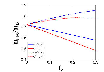
Figure 5: The ratio of the residual stress ($\Pi_{res}$) to the diffusive momentum flux ($\Pi_{D}$) as a function of $f_{Z}$. $\rm C^{6+}$ (red) and $\rm He^{2+}$ (blue) are considered. Dotted and solid lines represent the cases when $L_{eZ}=-1$ and 1, respectively. The quasi-linear momentum flux is calculated by integrating over all $k_{y}$ values giving rise to instability. Other plasma parameters being used are same as those of Fig. 2.

Figure 5 shows $R$ as a function of $f_{Z}$ for ${\rm C}^{6+}$ (red) and ${\rm He}^{2+}$ (blue) impurities. Plasma parameters being used to produce Fig. 5 are same as those of Fig. 2. In calculating the radial momentum flux in Figs. 5 and 6, we keep all the unstable modes in Eqs. (20), (21), and (22) by integrating over all $k_{y}$ giving rise to positive growth rate. $R$ shows a remarkably different trend depending on the alignment of an impurity profile to the main ion density profile. It increases when two profiles have a different sign (dotted lines) while it decreases when they have the same sign (solid lines). For example, the reduction in $R$ as $f_{Z}$ changes from $0$ to $0.15$ is $9.6\%$ and $16.6\%$ for $\rm{He}^{2+}$ and $\rm{C}^{6+}$ cases, respectively. For a same absolute value of $L_{eZ}$, the decrease rate of $R$ when $L_{eZ}>0$ is larger than the increase rate when $L_{eZ}<0$. Figure 6 highlights the impact of the profile alignment on $R$ for a fixed value of $f_{Z}=0.3$. The cyan dotted line in Fig. 6 represents the $R$ value when $f_{Z}=0$. It shows a considerable reduction from its reference value (dotted line) as $L_{ne}/L_{nZ}$ increases.

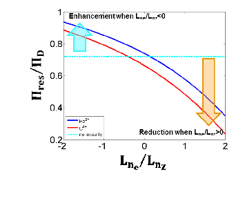
Figure 6: The ratio of the residual stress ($\Pi_{res}$) to the diffusive momentum flux ($\Pi_{D}$) as a function of $L_{eZ}=L_{n_{e}}/L_{n_{Z}}$. $\rm C^{6+}$ (red) and $\rm He^{2+}$ (blue) are considered with a fixed value of $f_{Z}=0.3$. A cyan dotted line represents the $\Pi_{res}/\Pi_{D}$ value without impurities. Other plasma parameters being used are same as those of Fig. 5.

To understand the results in Figs. 5 and 6, we evaluate $R$ for a fixed equilibrium velocity gradient and a $k_{y}$ value corresponding to the most unstable mode. Using the quasi-neutrality condition, Eq. (17) becomes

$$\Pi_{res}^{\rm{eff}} = \frac{1}{1+\hat{M}}\left(\frac{c_{s}\rho_{s}}{L_{n_{e}}}\right)^{2}\sum_{\vec{k}}\gamma\frac{k_{y}k_{\parallel}}{|\omega|^{2}}\frac{1}{1-f_{Z}}$$ (24)

$$\times \left\{1+\frac{2k_{y}\omega_{r}}{|\omega|^{2}}L_{ei}\left[K_{i}-f_{Z}\left(K_{i}-\frac{L_{eZ}}{L_{ei}}\frac{K_{Z}}{Z}\right)\right]\right\}|\phi_{k}|^{2},$$

where the relation $\hat{M}={m_{Z}n_{Z0}}/{m_{i}n_{i0}}=({\mu}/{Z})\left[{f_{Z}}/{1-f_{Z}}\right]$ is used. Next, noting that $\chi^{\rm{eff}}_{\phi}=(\chi^{i}_{\phi}+\hat{M}\chi^{Z}_{\phi})/(1+\hat{M})=\chi^{i}_{\phi}$ from Eq. (21), one can easily show that

$$\left<R\right>_{k_{y}}\sim\frac{1}{1+\hat{M}}\left<\frac{k_{\parallel}}{k_{y}}\right>\frac{1}{1-f_{Z}}\left\{1+\frac{2k_{y}\omega_{r}}{|\omega|^{2}}L_{ei}\left[K_{i}-f_{Z}\left(K_{i}-\frac{L_{eZ}}{L_{ei}}\frac{K_{Z}}{Z}\right)\right]\right\},$$ (25)

where $\left<R\right>_{k_{y}}$ denotes an ensemble averaged value of $R$ for a fixed $k_{y}$.

From the examination of Eq. (25), one can see that impurities affect $R$ through four ways:

• the mode shift which is contained in $\left<k_{\parallel}/k_{y}\right>$,

• impurity contents ($f_{Z}$),

• stability change by the change of the sign of $L_{eZ}$,

• the radial inhomogeneity of a impurity profile represented by $K_{Z}$, i.e., the direct impurity effect to the residual stress.

All the first three effects turn out to be important in the determination of $R$. Among them, the mode shift, which is presented in Fig. 4, is found to be the most crucial factor determining the amount of residual stress by the variation of $L_{eZ}$. The last term in Eq. (25) represents a driving term to the residual stress solely from the free energy of impurities, i.e., the radial inhomogeneity of an impurity profile. Positive $L_{eZ}$ makes the last term of Eq. (25) negative since $L_{ei}>0$ in nominal tokamak discharges and $\omega_{r}<0$. Thus, this term can further reduce $\left<R\right>_{k_{y}}$ combined with a strong reduction of $|X_{0}|$ when $L_{eZ}>0$. However, the effect of this term is marginal for cold impurity ions or high $Z$ impurities like $W^{46+}$ expected in machines with full tungsten PFCsAngioni-JET . However, this term may play a role in $\left<R\right>$ when fusion-born helium ashes are present because of their small charge number and natural tendency to align with main ions. Thus, results in this section might raise a potential concern to ITER operation where a significant amount of plasma rotation is envisioned to be produced via intrinsic rotation.

V Summary and conclusions

In conclusion, this paper has shown that impurities may change the amount of intrinsic rotation by affecting the residual stress driven by turbulence. To make an analytic study, we employed a two fluid model for ions and impurities for ITG turbulence in sheared slab geometry. The ion and impurity velocities are assumed to be equal, which is strictly valid in the collisional regime. Then, we evaluated the momentum diffusivity and the residual stress in a coupled main ion-impurity system. The principal findings of this paper are summarized as follows:

• Characteristics of ITG modes, such as the growth rate or the mode structure, changes significantly by the variation of impurities contents and/or the alignment of an impurity profile with that of main ions. Quasi-linear calculations show that these changes result in a considerable change of turbulence driven residual stress, hence the amount of intrinsic rotation.

• The ratio of residual stress ($\Pi_{res}$) to the diffusive momentum flux ($\Pi_{D}$), $R=\Pi_{res}/\Pi_{D}$, can be used as a quantitative measure of relative importance of $\Pi_{res}$ over $\Pi_{D}$.

• For a core-peaked impurity profile shown in Fig. 1(a) schematically, $R$ decreases due to the stabilization and a large increase of the mode shift of the unstable mode. For a wall-peaked impurity profile shown in Fig. 1(b) schematically, $R$ increases a little implying the predominance of $\Pi_{res}$ over $\Pi_{D}$. The degree of the enhancement of $R$ when $L_{eZ}<0$ is smaller than that of reduction when $L_{eZ}<0$ for a given impurity content.

As a possible implication of the present study, we pointed out that the amount of intrinsic rotation in burning plasma experiments might be reduced. This is due to the presence of ${\rm He^{2+}}$ ashes which is likely to be aligned with the main ion profile. For example, approximately $\sim 10\%$ of intrinsic rotation loss is expected if we assume the presence of $\rm{He}^{2+}$ ions with $f_{Z}=0.15$ well-aligned with a main ion profile. Such a well-aligned impurity profile is also possible in present day devices, as shown in recent experiments in KSTARKSTAR , due to the prevalence of turbulent impurity transport. We note that this may cause the decoupling of the ion temperature and the toroidal rotation profiles, which has been observed in recent KSTAR H-mode experimentsWKo . When $L_{eZ}>0$, the reduction of residual stress will be larger than that of the diffusive momentum flux. Since the intrinsic torque is believed to be maximized near the pedestal top region as shown in recent flux-driven gyrofluid simulationsJKPS ; Tokunaga , the reduction of the residual stress due to impurities will result in the reduction of a net intrinsic torque. This will reduce the total amount of toroidal rotation when an edge pedestal build up. To confirm this scenario, measurements of a rotation profile for a varying impurity contents is necessary. This is left as a future investigation.

As an extension of the present study, we plan to perform a gyrokinetic analysis including impurities. Nonlinear gyrokinetic or gyrofluid simulations are also planned to elucidate the nonlinear physical process of intrinsic rotation generation and saturation in the presence of impurities. These will be outstanding research subjects which will be published in the future.

- (1) D. G. Whyte, M. R.Wade, D. F. Finkenthal, K. H. Burrell, P. Monier-Garbet, B. W. Rice, D. P. Schissel, W. P. West, and R. D. Wood, Nucl. Fusion 38, 387 (1997).
- (2) H. H. Lee (private communication, 2014).
- (3) A. Kallenbach, R. Dux, M. Mayer, R. Neu, T. Pütterich, V. Bobkov, J. C. Fuchs, T. Eich, L. Giannone, O. Gruber, A. Herrmann, L. D. Horton, C. F. Maggi, H. Meister, H. W. Müller, V. Rohde, A. Sips, A. Stäbler, J. Stober, and ASDEX Upgrade Team, Nucl. Fusion 49, 045007 (2009).
- (4) F. Romanelli and JET EFDA Contributors, Nucl. Fusion 53, 104002 (2013).
- (5) G. Federici, P. Andrew, P. Barabaschi, J. Brooks, R. Doerner, A. Geier, A. Herrmann, G. Janeschitz, K. Krieger, A. Kukushkin, A. Loarte, R. Neu, G. Saibene, M. Shimada, G. Strohmayer, and M. Sugihara, J. Nucl. Mater. 313-316, 11 (2003).
- (6) D. Reiter, H. Kever, G. H. Wolf, M. Baelmans, R. Behrisch and R. Schneider, Plasma Phys. Control. Fusion, 33, 1579 (1991).
- (7) A. R. Polevoi, M. Shimada, M. Sugihara, Yu. L. Igitkhanov, V. S. Mukhovatov, A. S. Kukushkin, S. Yu. Medvedev, A. V. Zvonkov, and A.A. Ivanov Nucl. Fusion 45, 1451 (2005).
- (8) S. P. Hirshman and D. J. Sigmar, Nucl. Fusion 21, 1079 (1981).
- (9) Y. B. Kim, P. H. Diamond, and, R. J. Groebner, Phys. Fluids B 3, 2050 (1991).
- (10) R. Dux and A. G. Peeters, Nucl. Fusion 40, 1721 (2000).
- (11) X. Garbet, N. Dubuit, E. Asp, Y. Sarazin, C. Bourdelle, P. Ghendrih, and G. T. Hoang, Phys. Plasmas 12, 082511 (2005).
- (12) C. Angioni and A. G. Peeters, Phys. Rev. Lett. 96, 095003 (2006).
- (13) B. Coppi, H. P. Furth, M. N. Rosenbluth, and R. Z. Sagdeev, Phys. Rev. Lett. 17, 377 (1966).
- (14) J. Q. Dong, W. Horton, and W. Dorland, Phys. Plasmas 1, 3635 (1994).
- (15) J. Q. Dong, and W. Horton, Phys. Plasmas 2, 3412 (1995).
- (16) X. Y. Fu, J. Q. Dong, W. Horton, C. T. Ying, and G. J. Liu, Phys. Plasmas 4, 588 (1997).
- (17) T. Fülöp and J. Weiland, Phys. Plasmas 13, 112504 (2006).
- (18) C. Angioni, L. Carraro, T. Dannert, N. Dubuit, R. Dux, C. Fuchs, X. Garbet, L. Garzotti, C. Giroud, R. Guirlet, F. Jenko, O. J. W. F. Kardaun, L. Lauro-Taroni, P. Mantica, M. Maslov, V. Naulin, R. Neu, A. G. Peeters, G. Pereverzev, M. E. Puiatti, T. Pütterich, J. Stober, M. Valovič, M. Valisa, H. Weisen, A. Zabolotsky, ASDEX Upgrade Team, and JET EFDA Contributors, Phys. Plasmas 14, 055905 (2007).
- (19) H. Nordman, R. Singh, T. Fülöp, L.-G. Eriksson, R. Dumont, J. Anderson, P. Kaw, P. Strand, M. Tokar, and J. Weiland, Phys. Plasmas 15, 042316 (2008).
- (20) T. Fülöp and H. Nordman, Phys. Plasmas 16, 032306 (2009.
- (21) W. M. Tang, R. B. White, and P. N. Guzdar, Phys. Fluids 23, 167 (1980).
- (22) P. H. Diamond, C. J. McDevitt, Ö . D. Gürcan, T. S. Hahm, W. X. Wang, E. S. Yoon, I. Holod, Z. Lin, V. Naulin, and R. Singh, Nucl. Fusion 49, 045002 (2009).
- (23) P. H. Diamond, C. J. McDevitt, Ö . D. Gürcan, T. S. Hahm, and V. Naulin, Phys. Plasmas 15, 012303 (2008).
- (24) Ö. D. Gürcan, P. H. Diamond, T. S. Hahm, and R. Singh, Phys. Plasmas 14, 042306 (2007).
- (25) Ö. D. Gürcan, P. H. Diamond, P. Hennequin, C. J. McDevitt, X. Garbet, and C. Bourdelle, Phys. Plasmas 17, 112309 (2010).
- (26) C. J. McDevitt, P. H. Diamond, Ö. D. Gürcan, and T. S. Hahm, Phys. Rev. Lett, 103, 205003 (2009).
- (27) Rameswar Singh, Rajaraman Ganesh, Raghvendra Singh, Predhiman Kaw, and Abhijit Sen, Nucl. Fusion 51, 013002 (2011).
- (28) Rameswar Singh, R. Singh, Hogun Jhang and P. H. Diamond, Phys. Plasmas 21, 012302 (2014).
- (29) R. Balescu, Aspects of anomalous transport in plasmas, (IOP Publishing Ltd., Bristol, UK, 2005), p. 55.
- (30) P. Gohil, K. H. Burrell, and T. N. Carlstrom, Nucl. Fusion 38, 93 (1998).
- (31) N. C. Hawkes, D. V. Bartlett, D. J. Campbell, N. Deliyanakis, R. M. Gianella, P. J. Lomas, N. J. Peakcock, L. Porte, A. Rookes, and P. R. Thomas, Plasma Phys. Control. Fusion 38, 1261 (1996).
- (32) L. Wang and P.H. Diamond, Phys. Rev. Lett. 110, 265006 (2013).
- (33) X. Garbet, D. Esteve, Y. Sarazin, J. Abiteboul, C. Bourdelle, G. Dif-Pradalier, P. Ghendrih, V. Grandgirard, G. Latu, and A. Smolyakov, Phys. Plasmas 20, 072502 (2013).
- (34) Won-Ha Ko, H. Lee, P.H. Diamond, S.H. Ko, J.M. Kwon, L. Terzolo, S. Oh, K. Ida, Y.M. Jeon, K.D.Lee, J.H. Lee, S.W. Yoon, Y.S. Bae, W.C. Kim, Y.K. Oh, and J.G. Kwak, in Proceedings of the 24th IAEA Fusion Energy Conference, San Diego, USA, October 8-13, 2012 (International Atomic Energy Agency, Vienna, 2012), PD/P8-22.
- (35) Hogun Jhang, S. S. Kim, and P. H. Diamond, Jour. Kor. Phys. Soc. 61, 55 (2012).
- (36) S. Tokunaga, Hogun Jhang, S. S. Kim, and P. H. Diamond, Phys. Plasmas 19, 092303 (2012).