Monte Carlo Motion Planning for Robot Trajectory Optimization Under Uncertainty

Abstract

This article presents a novel approach, named MCMP (Monte Carlo Motion Planning), to the problem of motion planning under uncertainty, i.e., to the problem of computing a low-cost path that fulfills probabilistic collision avoidance constraints. MCMP estimates the collision probability (CP) of a given path by sampling via Monte Carlo the execution of a reference tracking controller (in this paper we consider LQG). The key algorithmic contribution of this paper is the design of statistical variance-reduction techniques, namely control variates and importance sampling, to make such a sampling procedure amenable to real-time implementation. MCMP applies this CP estimation procedure to motion planning by iteratively (i) computing an (approximately) optimal path for the deterministic version of the problem (here, using the FMT${}^{*}\,$algorithm), (ii) computing the CP of this path, and (iii) inflating or deflating the obstacles by a common factor depending on whether the CP is higher or lower than a target value. The advantages of MCMP are threefold: (i) asymptotic correctness of CP estimation, as opposed to most current approximations, which, as shown in this paper, can be off by large multiples and hinder the computation of feasible plans; (ii) speed and parallelizability, and (iii) generality, i.e., the approach is applicable to virtually any planning problem provided that a path tracking controller and a notion of distance to obstacles in the configuration space are available. Numerical results illustrate the correctness (in terms of feasibility), efficiency (in terms of path cost), and computational speed of MCMP.

1 Introduction

Robotic motion planning is the problem of computing a path that connects an initial and a terminal robot state while avoiding collisions with obstacles and optimizing an objective function LaValle (2006). Despite the fact that finding a feasible, let alone optimal, solution to a motion planning problem is difficult (even the most basic versions of the problem are already PSPACE-hard Reif (1979); LaValle (2006)), in the past three decades key breakthroughs have made the solution to this problem largely practical (see LaValle (2006) and references therein for a comprehensive historical account). Most works in the literature, however, focus on a deterministic setup where the state of a robot is perfectly known and its actions lead to a deterministic, unique outcome. While this is usually an excellent approximation for robots operating in highly structured environments (e.g., manipulators in an assembly line), it falls short in unstructured settings, e.g., for ground or aerial field robots or surgical robotic systems LaValle (2011). In such cases, motion uncertainty, sensing uncertainty, and environment uncertainty may dramatically alter the safety and quality of a path computed via deterministic techniques (i.e., neglecting uncertainty). Hence, accounting for uncertainty in the planning process is regarded as an essential step for the deployment of robotic systems “outside the factory floor” LaValle (2011). In this paper we introduce Monte Carlo Motion Planning, a novel approach to planning under uncertainty that is accurate, fast, and general.

Related work: Conceptually, to enable a robot to plan its motion under uncertainty, one needs to design a strategy for a decision maker. In this regard, robotic motion planning can be formalized as a partially observable Markov decision process (POMDP) Kaelbling et al. (1998), where the key idea is to assume that the state evolves according to a controlled Markov chain, the state is only partially observed, and one seeks to design a control policy that maps state probability distributions to actions. However, despite the theoretical Kaelbling et al. (1998) and practical Kurniawati et al. (2008) successes of the POMDP theory, the online computation of a control policy for robotic applications is extremely computationally intensive, and possibly even unnecessary as after a short time horizon the environment map may have changed LaValle (2006). The alternative and widely adopted approach is then to restrict the optimization process to open-loop trajectories, which involves the much simpler task of computing a control sequence (as opposed to a control policy), and recompute the reference trajectory in a receding horizon fashion (e.g., every few seconds). This is the approach we consider in this paper.

To select open-loop trajectories, a large number of works cast the problem into a chance-constrained optimization problem Blackmore et al. (2010), where under the assumption of linear dynamics and convex obstacles, an open-loop control sequence is computed as the solution to a mixed-integer linear program. The works in Vitus and Tomlin (2011); Ono et al. (2013) extend this approach to an optimization over the larger class of affine output feedback controllers, comprising a nominal control input and an error feedback term. These works, however, require an explicit characterization of the obstacle space (in the configuration space), which is oftentimes unavailable (LaValle, 2006, Chapter 5). This has prompted a number of researchers to extend the sampling-based motion planning paradigm to the problem of planning under uncertainty (in the sampling-based paradigm, an explicit construction of the configuration space is avoided and the configuration space is probabilistically “probed” with a sampling scheme LaValle (2006)). A common approach is to forgo path optimization and recast the problem as an unconstrained planning problem where the path collision probability (CP) is minimized. For example, the approach of LQG-MP Berg et al. (2011) is to approximate a path CP by combining pointwise CPs as if they were independent, running the rapidly-exploring random trees (RRT) LaValle and Kuffner (2001) algorithm multiple times, and then selecting the path with minimum (approximate) path CP. The pointwise CPs are computed within the model that a reference tracking controller is employed to track a nominal open-loop path. This is closely related to model predictive control (MPC) with closed-loop prediction Oldewurtel et al. (2008) and leads to a less conservative collision probability estimate than if the nominal control was executed without feedback. A similar approach is used in Sun et al. (2013), where the authors employ a truncation method Patil et al. (2012) to improve the accuracy of path CP computation.

The interplay between minding collision probability while simultaneously optimizing a path planning cost objective function is considered in Sun et al. (2015), although still with an approximation to the path CP. There, cost optimization is considered over the set of path plans satisfying a lower bound on success probability. The inclusion of path CP as a constraint is also considered in Luders et al. (2010), where the authors propose CC-RRT, an RRT-based algorithm that approximates path CP via Boole’s bound. CC-RRT has been extended to include dynamic obstacles via Bayesian nonparametric models Aoude et al. (2013), tailored to the control of unmanned aerial vehicles Kothari and Postlethwaite (2013) and parafoils Luders et al. (2013b), and combined with the RRT* asymptotically optimal version of RRT Luders et al. (2013a).

Contributions: In this paper we present an algorithm for robot planning under uncertainty that returns high quality solutions (in terms of a general planning objective) which satisfy a specified constraint on collision probability, or safety tolerance. The motivation of this work is that all of the aforementioned approaches approximate path CP in ways that can be quite inaccurate, thus potentially drastically mischaracterizing the feasible domain of path optimization. In particular, we show (see Figure 2) that those approximations can be off by many multiples in simple examples. To address this problem, our first contribution is to design a variance-reduced (that is, quickly-converging) Monte Carlo (MC) probability estimation algorithm for CP computation. This algorithm estimates the collision probability of a given trajectory by sampling many realizations of a reference-tracking controller, modeling the effort of a robot to follow a reference path. In particular, in this paper, we assume a Linear-Quadratic Gaussian (LQG) tracking controller, similar to LQG-MP Berg et al. (2011) and MPC with closed-loop prediction Oldewurtel et al. (2008). Our algorithm does not suffer the inaccuracies of the approximations mentioned earlier, and indeed provides the exact path CP given enough time (in contrast to current approaches). Most importantly, our variance-reduction scheme, which combines and tailors control variate and importance sampling techniques in an original fashion to the problem at hand, enables the computation of very accurate estimates in a way compatible with real-time operations. This holds even when working with very small CPs, a regime in which a straightforward Monte Carlo method would require great computational expense to arrive at accurate estimates. Another key advantage of our algorithm is that it comes with an estimate of its variance, so that we have a measure of accuracy, unlike the aforementioned approximations. It is also trivially parallelizable and has the potential to be extended to very general controllers and uncertainty models.

Our estimation algorithm enables a novel approach to planning under uncertainty, which we call Monte Carlo Motion Planning (MCMP)—our second contribution. MCMP proceeds by performing bisection search over CP and obstacle inflation, at each step solving a deterministic version of the problem with inflated obstacles. To demonstrate the performance of MCMP, we present simulation results that illustrate the correctness (in terms of feasibility), efficiency (in terms of path cost), and computational speed of MCMP. From a conceptual standpoint, MCMP can be viewed as a planning analogue to MC approaches for robot localization Thrun et al. (2001).

Organization: This paper is structured as follows. Section 2 reviews some background on MC variance reduction. Section 3 formally defines the problem we consider in this paper. Section 4 elucidates the shortcomings of previous path CP approximation schemes. Section 5 presents variance-reduction techniques for fast MC computation of path CP. Section 6 presents the overall MCMP approach. Section 7 presents results from numerical experiments supporting our statements. Finally, in Section 8, we draw some conclusions and discuss directions for future work.

2 Background on Monte Carlo Variance Reduction

The use of Monte Carlo (MC) to estimate the probability of complex events is well-studied. In this section we will briefly introduce MC and the two variance reduction techniques that provide the basis for our main result in Section 5. For more detail and other topics on Monte Carlo, the reader is referred to the excellent unpublished text Owen (2013), from which the material of this section is taken.

2.1 Simple Monte Carlo

In its most general form, MC is a way of estimating the expectation of a function of a random variable by drawing many independent and identically distributed (i.i.d.) samples of that random variable, and averaging their function values. Explicitly, consider a random variable $\bm{X}\in\mathbb{R}^{n}$ and a bounded function $f:\mathbb{R}^{n}\rightarrow\mathbb{R}$. For a sequence of $m$ i.i.d. realizations of $\bm{X}$, $\{\bm{X}^{(i)}\}_{i=1}^{m}$, the central limit theorem gives,

$$\sqrt{m}\left(\frac{1}{m}\sum_{i=1}^{m}f\left(\bm{X}^{(i)}\right)-\mathbb{E}\left[f\left(\bm{X}\right)\right]\right)\stackrel{{\scriptstyle\mathcal{D}}}{{\longrightarrow}}N\left(0,\tau^{2}\right),$$ (1)

as $m\rightarrow\infty$, where $\stackrel{{\scriptstyle\mathcal{D}}}{{\longrightarrow}}$ denotes convergence in distribution, and $N(0,\tau^{2})$ refers to the Gaussian distribution with mean $0$ and variance $\tau^{2}$. This implies $\frac{1}{m}\sum_{i=1}^{m}f\left(\bm{X}^{(i)}\right)\stackrel{{\scriptstyle p}}{{\longrightarrow}}\mathbb{E}\left[f\left(\bm{X}\right)\right]$ as $m\rightarrow\infty$, where $\stackrel{{\scriptstyle p}}{{\longrightarrow}}$ denotes convergence in probability.

In this paper, $\bm{X}$ will be a random trajectory controlled to follow a nominal path, and $f$ will be the indicator function that a trajectory collides with an obstacle; call this collision event $A$. Therefore, the expectation in Equation (1) is just $\mathbb{E}[f(\bm{X})]=\mathbb{P}(A)$. Denote this collision probability by $p$, and define $\hat{p}_{\text{simple}}:=\frac{1}{m}\sum_{i=1}^{m}f\left(\bm{X}^{(i)}\right)$. Then $\tau^{2}$ can be consistently estimated by the sample variance of the $f(\bm{X}^{(i)})$,

$$\hat{\tau}^{2}:=\frac{1}{m}\sum_{i=1}^{m}\left(f\left(\bm{X}^{(i)}\right)-\hat{p}_{\text{simple}}\right)^{2}\stackrel{{\scriptstyle p}}{{\longrightarrow}}\tau^{2},$$ (2)

as $m\rightarrow\infty$. $\hat{V}_{\text{simple}}:=\hat{\tau}^{2}/m$ allows us to quantify the uncertainty in the CP estimator $\hat{p}_{\text{simple}}$ by approximating its variance. The material from this subsection can be found with more detail in (Owen, 2013, Chapter 2).

2.2 Control Variates

To reduce the variance of $\hat{p}_{\text{simple}}$, we can use the method of control variates (CV). CV requires a function $h:\mathbb{R}^{n}\rightarrow\mathbb{R}$ such that $\theta:=\mathbb{E}[h(\bm{X})]$ is known. Then if $h(\bm{X}^{(i)})$ is correlated with $f(\bm{X}^{(i)})$, its variation around its (known) mean can be used to characterize the variation of $f(\bm{X}^{(i)})$ around its (unknown) mean, which can then be subtracted off from $\hat{p}_{\text{simple}}$. Explicitly, given a scaling parameter value $\beta$, we estimate $p=\mathbb{E}[f(\bm{X})]$ by,

$$\hat{p}_{\beta}:=\frac{1}{m}\sum_{i=1}^{m}(f(\bm{X}^{(i)})-\beta h(\bm{X}^{(i)}))+\beta\theta=\hat{p}_{\text{simple}}-\beta(\hat{\theta}-\theta),$$ (3)

where $\hat{\theta}$ is the sample average of the $h(\bm{X}^{(i)})$. The optimal (variance-minimizing) choice of $\beta$ can be estimated from the simulated data as

$$\hat{\beta}:=\sum_{i=1}^{m}(f(\bm{X}^{(i)})-\hat{p}_{\text{simple}})(h(\bm{X}^{(i)})-\hat{\theta})\Big{/}\sum_{i=1}^{m}(h(\bm{X}^{(i)})-\hat{\theta})^{2}.$$ (4)

We then use the CP estimator $\hat{p}_{\hat{\beta}}$, whose variance can be estimated by,

$$\hat{V}_{\hat{\beta}}:=\frac{1}{m^{2}}\sum_{i=1}^{m}(f(\bm{X}^{(i)})-\hat{p}_{\hat{\beta}}-\hat{\beta}(h(\bm{X}^{(i)})-\hat{\theta}))^{2}.$$ (5)

The data-dependent choice of $\beta$ introduces a bias in $\hat{p}_{\hat{\beta}}$ that is asymptotically (in $m$) negligible compared to its variance, so we will ignore it here. As $m\rightarrow\infty$, the variance reduction due to CV can be characterized by $\operatorname{Var}(\hat{p}_{\hat{\beta}})/\operatorname{Var}(\hat{p}_{\text{simple}})\rightarrow 1-\rho^{2}$, where $\rho$ is the correlation between $f(\bm{X})$ and $h(\bm{X})$. The material from this subsection can be found with more detail in (Owen, 2013, Section 8.9).

2.3 Importance Sampling

When $f(\bm{X})$ is the indicator function for a rare event $A$, as it is in this paper (we assume that in most settings, path CP constraints will be small to ensure a high likelihood of safety), MC variance reduction is often needed, with importance sampling (IS) a particularly useful tool. Since $p\ll 1$, we can approximate the coefficient of variation (ratio of standard deviation to expected value) of the estimator $\hat{p}_{\text{simple}}$ as,

$$\frac{\sqrt{\operatorname{Var}(\hat{p}_{\text{simple}})}}{\mathbb{E}[\hat{p}_{\text{simple}}]}=\frac{\sqrt{p(1-p)/m}}{p}\approx\frac{1}{\sqrt{m}}\frac{1}{\sqrt{p}}.$$ (6)

This means that in order to get the relative uncertainty in $\hat{p}_{\text{simple}}$ to be small, one needs $m\gg 1/p$ which can be very large, and this is simply due to the rarity of observing the event $A$. IS allows us to sample $\bm{X}$ from a distribution that makes the event $A$ more common and still get an unbiased estimate of $p$.

Until now we have considered $\bm{X}$ to have some fixed probability density function (pdf) $P:\mathbb{R}^{n}\rightarrow\mathbb{R}_{\geq 0}$. Denoting the expectation of $f(\bm{X})$ when $\bm{X}$ has pdf $P$ by $\mathbb{E}_{P}[f(\bm{X})]$, then for any pdf $Q$ whose support contains that of $P$ (that is, $P(\bm{x})>0\Rightarrow Q(\bm{x})>0$),

$$\mathbb{E}_{P}[f(\bm{X})]=\int_{\mathbb{R}^{n}}f(\bm{x})P(\bm{x})d\bm{x}=\int_{\mathbb{R}^{n}}f(\bm{x})\frac{P(\bm{x})}{Q(\bm{x})}Q(\bm{x})d\bm{x}=\mathbb{E}_{Q}\left[f(\bm{X})\frac{P(\bm{X})}{Q(\bm{X})}\right]$$

Therefore, letting $\{\tilde{\bm{X}}^{(i)}\}_{i=1}^{m}$ be i.i.d. samples with pdf $Q$, the IS estimate and associated variance estimate are,

$$\hat{p}_{Q}:=\frac{1}{m}\sum_{i=1}^{m}\frac{f(\tilde{\bm{X}}^{(i)})P(\tilde{\bm{X}}^{(i)})}{Q(\tilde{\bm{X}}^{(i)})},\qquad\quad\hat{V}_{Q}:=\frac{1}{m^{2}}\sum_{i=1}^{m}\left(\frac{f(\tilde{\bm{X}}^{(i)})P(\tilde{\bm{X}}^{(i)})}{Q(\tilde{\bm{X}}^{(i)})}-\hat{p}_{Q}\right)^{2}.$$ (7)

If $Q$ can be chosen in such a way that $A$ is common and the likelihood ratio $P(\bm{X})/Q(\bm{X})$ does not have high variance for $\bm{X}\in A$, then $\operatorname{Var}(\hat{p}_{Q})$ can be much smaller (orders of magnitude) than $\operatorname{Var}(\hat{p}_{\text{simple}})$ for the same $m$. The material from this subsection can be found with more detail in (Owen, 2013, Chapter 9).

2.4 Comments

CV and IS may be combined into one estimator, summarized in Algorithm 1, the full mathematical details of which are contained in (Owen, 2013, Section 9.10). Although CV and IS can both be excellent frameworks for variance reduction in MC, there is no general method for selecting $h$ or $Q$, and good choices for either one are extremely problem-dependent. Indeed, the main contribution of this paper is to find, for the important case of linear dynamics and Gaussian noise, $h$ and $Q$ that make MC estimation of CPs converge fast enough for real-time planning.

3 Problem Statement

We pose the problem of motion planning under uncertainty with safety tolerance as a constraint separate from the path cost to be optimized. We consider robots described by linear dynamics with control policies derived as LQG controllers tracking nominal trajectories. These nominal trajectories are planned assuming continuous dynamics, but in order to make the computation of path CPs tractable, we assume discretized (zero-order hold) approximate dynamics for the tracking controllers The full details of the continuous vs. discrete problem formulations are rather standard and due to space limitations are provided in Appendix A of the extended version of this paper Janson et al. (2015). Briefly here, with $\mathcal{N}(\mu,\Sigma)$ denoting a multivariate Gaussian with mean $\mu$ and covariance matrix $\Sigma$, the system dynamics are given by

$$\mathbf{x}_{t+1}=A\mathbf{x}_{t}+B\mathbf{u}_{t}+\mathbf{v}_{t},\quad\mathbf{v}_{t}\sim\mathcal{N}(\mathbf{0},V),\quad\mathbf{y}_{t}=C\mathbf{x}_{t}+\mathbf{w}_{t},\quad\mathbf{w}_{t}\sim\mathcal{N}(\mathbf{0},W).$$ (8)

where $\mathbf{x}_{t}\in{\mathbb{R}}^{d}$ is the state, $\mathbf{u}_{t}\in{\mathbb{R}}^{\ell}$ is the control input, $\mathbf{y}_{t}$ is the workspace output, and $\mathbf{v}_{t}$ and $\mathbf{w}_{t}$ represent Gaussian process and measurement noise, respectively. With deviation variables from a nominal trajectory defined as $\delta\mathbf{x}_{t}:=\mathbf{x}_{t}-\mathbf{x}^{\text{nom}}_{t}$, $\delta\mathbf{u}_{t}:=\mathbf{u}_{t}-\mathbf{u}^{\text{nom}}_{t}$, and $\delta\mathbf{y}_{t}:=\mathbf{y}_{t}-\mathbf{y}^{\text{nom}}_{t}$, for $t=0,\dots,T$, the discrete LQG controller $\delta\mathbf{u}^{\text{LQG}}_{t}:=L_{t}\,\widehat{\delta}\mathbf{x}_{t}$, with $L_{t}$ and $\widehat{\delta}\mathbf{x}_{t}$ denoting the feedback gain matrix and Kalman state estimate respectively, minimizes the tracking cost function

$$J:=\mathbb{E}\left[\delta\mathbf{x}_{T}^{T}F\delta\mathbf{x}_{T}+\sum_{t=0}^{T-1}\delta\mathbf{x}_{t}^{T}Q\delta\mathbf{x}_{t}+\delta\mathbf{u}_{t}^{T}R\delta\mathbf{u}_{t}\right].$$

The computation details of $L_{t}$ and the dynamics of $\widehat{\delta}\mathbf{x}_{t}$ are standard and given in Appendix A Janson et al. (2015); in the remainder of this paper we use only the notation that the combined state/estimate deviations evolve as multivariate Gaussians $\left[\delta\mathbf{x}_{t};\widehat{\delta}\mathbf{x}_{t}\right]\sim\mathcal{N}\left(\mu_{t},\Sigma_{t}\right)$ and for suitable definitions of $M_{t}$ and $N_{t}$ we may write

$$\begin{bmatrix}\delta\mathbf{x}_{t+1}\\ \widehat{\delta}\mathbf{x}_{t+1}\end{bmatrix}\sim\mathcal{N}\left(\mu_{t+1}=M_{t}\mu_{t},\Sigma_{t+1}=M_{t}\Sigma_{t}M_{t}^{T}+N_{t}\right).$$ (9)

Let $\mathcal{X}_{\text{obs}}$ be the obstacle space, so that $\mbox{$\mathcal{X}_{\text{free}}$}:={\mathbb{R}}^{d}\backslash\mbox{$\mathcal{X}_{\text{obs}}$}$ is the free space. Let $\mbox{$\mathcal{X}_{\text{goal}}$}\subset\mbox{$\mathcal{X}_{\text{free}}$}$ and $\mbox{$\bm{x}_{0}$}\in\mbox{$\mathcal{X}_{\text{free}}$}$ be the goal region and initial state. Given a path cost measure $c$ and letting $\overline{\mathbf{x}_{0},\dots,\mathbf{x}_{T}}$ denote the continuous curve traced by the robot’s random trajectory (connecting the waypoints $\mathbf{x}_{0},\dots,\mathbf{x}_{T}$) we wish to solve

Discretized stochastic motion planning (SMP):

$$\begin{split}\min_{\mathbf{u}^{\text{nom}}(\cdot)}&\quad c(\mathbf{x}^{\text{nom}}(\cdot))\\ \text{s.t.}&\quad\mathbb{P}\left(\overline{\mathbf{x}_{0},\dots,\mathbf{x}_{T}}\cap\mbox{$\mathcal{X}_{\text{obs}}$}\neq\varnothing\right)\leq\alpha\\ &\quad\mathbf{u}_{t}=\mathbf{u}^{\text{nom}}_{t}+\delta\mathbf{u}^{\text{LQG}}_{t}\\ &\quad\mathbf{x}_{0}\sim\mathcal{N}(\mathbf{x}^{\text{nom}}_{0},P_{0}),\quad\mathbf{x}_{T}\in\mbox{$\mathcal{X}_{\text{goal}}$}\\ &\quad\text{Equation \eqref{eqn:DLQG}}.\end{split}$$ (10)

Note that the optimization is still over continuous-time nominal paths, which we discretize when computing the path collision probability $\mathbb{P}\left(\overline{\mathbf{x}_{0},\dots,\mathbf{x}_{T}}\cap\mbox{$\mathcal{X}_{\text{obs}}$}\neq\varnothing\right)$.

This formulation is inspired by Oldewurtel et al. (2008); Berg et al. (2011) and represents a compromise between a POMDP formulation involving a minimization over the class of output-feedback control laws, and an open-loop formulation, in which the state is assumed to evolve in an open loop (i.e., no tracking). This can be justified in two ways. One is that the general constrained POMDP formulation is vastly more complex than ours and would require much more computation. The other is that, in practice, a motion plan is executed in a receding horizon fashion, so that computing output-feedback policies may not even be useful, since after a short time-horizon the environment map may have changed, requiring recomputation anyway. We note that the problem formulation could be readily generalized to a nonlinear setup and to any tracking controller (e.g., LQG with extended Kalman filter estimation is essentially already in the same form)—indeed, one of the key advantages of the MC approach is that it is able to handle (at least theoretically) such general versions of the problem. However, in the present paper, we limit our attention to the aforementioned LQG setup.

In the remainder of the paper, we discuss how to quickly and consistently (i.e., in a way that is asymptotically exact as the discretization step $\Delta t\to 0$) estimate the path CP appearing in equation (10), and then we will employ MCMP to generate approximate solutions to the discretized SMP problem.

4 The Problem of Computing Path CP

In general, the key difficulty for planning under uncertainty (provided a probabilistic uncertainty model is given) is to accurately compute path CP. All previous approaches essentially rely on two approaches, namely:

• Additive approach, e.g., Luders et al. (2010): using Boole’s inequality, i.e., $\mathbb{P}\left(\cup_{i}A_{i}\right)\leq\sum_{i}\mathbb{P}\left(A_{i}\right),$ by which a path CP is approximated by summing pointwise CP_i at a certain number of waypoints along the path, i.e., $\text{CP}\approx\sum_{i}\text{CP}_{i}$.

• Multiplicative approach, e.g., Berg et al. (2011): a path CP is approximated by multiplying the complement of point-wise CP_i, specifically $\text{CP}\approx 1-\prod_{i}(1-\text{CP}_{i})$.

There are three approximations inherent in both approaches:

1. The path CP is approximated by combining waypoint CP_i’s. That is, no accounting is made for what happens in between waypoints.

2. The waypoint CP_i’s are combined in an approximate manner. That is, in general there is a complex high-dimensional dependence between collisions at different waypoints, and these are not accounted for in either approach. In particular, the additive approach treats waypoint collisions as mutually exclusive, while the multiplicative approach treats them as independent. Since neither mutual exclusivity nor independence hold in general, this constitutes another approximation.

3. Each waypoint CP_i is approximated (e.g., by using a nearest obstacle). This is usually done because integrating a multivariate density over an intersection of half-planes (defining the obstacle set) can be quite computationally expensive.

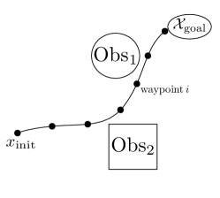
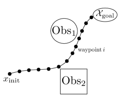
Figure 1: Illustration of the interplay between approximations (A) and (B). In (a), there are not enough waypoints to properly characterize the pathwise CP, while in (b), the waypoints may be too close to not account for their dependence.

A fundamental limitation in both approaches comes from the interplay between approximations (A) and (B). Specifically, while approximation (A) improves with higher-resolution waypoint placement along the path, approximation (B) actually gets worse, see Figure 1. In Figure 1, although Obs₂ comes very close to the path, it does not come very close to any of the waypoints, and thus the pathwise CP will not be properly accounted for by just combining pointwise CPs. In Figure 1, the waypoints closest to Obs₁ will have highly-correlated CPs, which again is not accounted for in either the additive or multiplicative approaches. For the linear Gaussian setting considered here, as the number of waypoints along a fixed path goes to infinity, the path CP estimate from the additive approach actually tends to $\infty$, while that of the multiplicative approach tends to 1, regardless of the true path CP. To see this, note that for any fixed path, there exists a positive number $\epsilon>0$ such that CP_i is larger than or equal to $\epsilon$ for any point on the path. Therefore,

$$\sum_{i=1}^{k}\text{CP}_{i}\geq k\,\epsilon\stackrel{{\scriptstyle k\rightarrow\infty}}{{\longrightarrow}}\infty,\qquad\;1\geq 1-\prod_{i=1}^{k}(1-\text{CP}_{i})\geq 1-(1-\epsilon)^{k}\stackrel{{\scriptstyle k\rightarrow\infty}}{{\longrightarrow}}1,$$ (11)

where $k$ is the number of waypoints. In other words, both approaches are asymptotically tautological, as they upper-bound a probability with a number greater than or equal to one. An important consequence of this is that as the number of waypoints approaches infinity, either approach would deem all possible paths infeasible with respect to any fixed non-trivial path CP constraint. This point is emphasized in Figure 2, which compares true path CP to approximations computed using the additive and multiplicative approaches for two different paths, as a function of the number of waypoints along the path. Off the plotted area, the additive approach passes through an approximate probability of 1 and continues to infinity, while the multiplicative approach levels off at 1. Even with few waypoints, both approaches are off by hundreds of percent. The overly conservative nature of the multiplicative approach has been recognized in Patil et al. (2012), where the authors replace approximate marginal pointwise CPs in the multiplicative approach with approximate pointwise CPs conditional on the previous waypoint being collision-free. While this is a first-order improvement on the standard approaches, the conditional pointwise probabilities are quite complex but are approximated by Gaussians for computational reasons, with the result that their approximate path CPs can still be off by many multiples of the true value, especially for small path CPs (which will usually be the relevant ones). The red curve in Figure 2 and 2 shows that the approximation of Patil et al. (2012), while a substantial improvement over the alternatives, can still be off by factors of 5 or more, and the discrepancy appears to be increasing steadily with the number of waypoints.

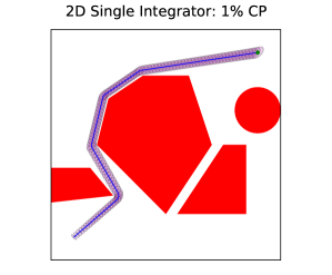
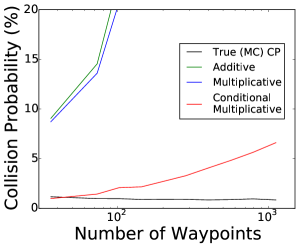
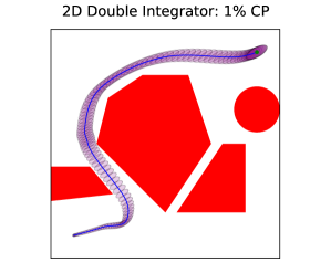
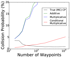
Figure 2: Illustration of path CP approximation schemes for two robotic systems where the true path CP is around 1% under the continuous controller. In (a) and (c), the blue curve represents the nominal path, the red boxes are the obstacles, and the purple ellipses represent 95% pointwise marginal confidence intervals at individual waypoints at discretizations with 102 and 104 points respectively. Panels (b) and (d) show the collision probability estimated by each approximation scheme as a function of the number of waypoints. Approximation (C) in all approaches is matched to their respective papers (additive: Luders et al. (2010); Aoude et al. (2013); Kothari and Postlethwaite (2013); Luders et al. (2013a), multiplicative: Berg et al. (2011), conditional multiplicative: Patil et al. (2012); Sun et al. (2013); Liu and Ang (2014)).

A few comments are in order. First, there is nothing pathological in the example in Figure 2, as similar results are obtained with other obstacle configurations and in higher dimensions. Second, we note that approximations such as these may be very useful for unconstrained problems that penalize or minimize path CP, since they may measure the relative CP between paths well, even if they do not agree with the true path CP in absolute terms. However, to address the chance-constrained SMP, one needs an accurate (in absolute terms) and fast method to estimate path CP, which is one of the key contributions of this paper. Third, the additive approach is guaranteed to be conservative with respect to approximation (B). That is, ignoring (A) and (C) (the latter of which can also be made conservative), the additive approach will produce an overestimate of the path CP. Although this can result in high-cost paths or even problem infeasibility, it is at least on the safe side. This guarantee comes at a cost of extreme conservativeness, and the two less-conservative multiplicative approaches have no such guarantee for any finite number of waypoints. Fourth, the limits in equation (11) apply to any uncertainty model supported on the entire configuration space, and even to bounded uncertainty models so long as the path in question has a positive-length segment of positive pointwise CP.

In the next section, we will present a MC approach that addresses all three approximations (A)-(C) stated earlier. Specifically, for (A), although collisions can truly be checked along a continuous path only for special cases of obstacles, Monte Carlo simply checks for collisions along a sampled path and thus can do so at arbitrary resolution, regardless of the resolution of the actual waypoints, so approximation (A) for MC has no dependence on waypoint resolution. For (B), the high-dimensional joint distribution of collisions at waypoints along the path is automatically accounted for when sampling entire realizations of the tracking controller. And for (C), since MC only has to check for collisions at specific points in space, no multivariate density integration needs to be done.

5 Variance-Reduced Monte Carlo for Computing Pathwise CP

5.1 Control Variates

As discussed in Section 2.2, a good control variate $h$ for $f$ should have a known (or rapidly computable) expected value, and should be highly correlated with $f$. As mentioned in the previous section, existing probability-approximation methods, while not accurate in absolute terms, can act as very good proxies for CP in that they resemble a monotone function of the CP. Coupled with the fact that such approximations are extremely fast to compute, they make ideal candidates for $h$.

Since even individual waypoint CPs are expensive to compute exactly for all but the simplest obstacle sets, we approximate the obstacle set locally as a union of half-planes, similar to Patil et al. (2012). For each waypoint $\mathbf{x}^{\text{nom}}_{t}$ along the nominal path, we compute the closest obstacle points $\mathbf{z}_{t}^{(i)}$ and their corresponding obstacle half-planes such that none of these points are occluded by each others’ half-planes. “Close” is measured in terms of the Mahalanobis distance defined by the covariance matrix of the robot state at that waypoint, and the obstacle half-planes are defined as tangent to the multivariate Gaussian density contour at each close point. Mathematically this corresponds to at most one point per convex obstacle region $\mbox{$\mathcal{X}_{\text{obs}}$}^{(i)}$ (with $\mbox{$\mathcal{X}_{\text{obs}}$}=\bigcup_{i=1}^{M}\mbox{$\mathcal{X}_{\text{obs}}$}^{(i)}$), i.e.,

$$\mathbf{z}_{t}^{(i)}=\operatorname*{arg\,min}_{\mathbf{a}\in\mbox{$\mathcal{X}_{\text{obs}}$}^{(i)}}(\mathbf{a}-\mathbf{x}^{\text{nom}}_{t})^{T}\Sigma_{t}^{-1}(\mathbf{a}-\mathbf{x}^{\text{nom}}_{t}).$$

We then approximate the pointwise probability of collision by the probability of crossing any one of these half-planes; this probability is approximated in turn by Boole’s bound so that an expectation is simple to compute. That is, we define $h_{ti}(\bm{X})$ to be the indicator that $\mathbf{x}^{\text{nom}}_{t}$ crosses the $\mathbf{z}_{t}^{(i)}$ obstacle half-plane, and define $h(\bm{X})=\sum_{t,i}h_{ti}(\bm{X})$. We note that considering multiple close obstacle points, as opposed to only the closest one, is important when planning in tight spaces with obstacles on all sides. Correlations between $h$ and $f$ in testing were regularly around 0.8.

5.2 Importance Sampling

From a statistical standpoint, the goal in selecting the importance distribution $Q$ is to make the pathwise CP sampled under $Q$ on the order of 1, while keeping the colliding paths sampled from $Q$ as likely as possible under the nominal distribution $P$. From a computational standpoint, we want $Q$ to be fast to sample from and for the likelihood ratio $P/Q$ to be easy to compute. Our method for importance sampling constructs $Q$ as a mixture of sampling distributions $Q_{0},...,Q_{K}$—one for each close obstacle point $\mathbf{z}_{t}^{(i)}$ along the nominal trajectory. The intent of distribution $Q_{ti}$ is to sample a path that is likely to collide with the obstacle set at waypoint $t$. We accomplish this by shifting the means of the noise distributions $\mathbf{n}_{s}$, $0\leq s\leq t$, leading up to time $t$ so that $\mathbb{E}_{Q_{ti}}[\delta\mathbf{x}_{t}]=\mathbf{z}_{t}^{(i)}-\mathbf{x}_{t}^{\text{nom}}$. To minimize likelihood ratio $P(\bm{X})/Q_{ti}(\bm{X})$ variance, we distribute the shift in the most likely manner according to Mahalanobis distance. This amounts, through Equation (9), to solving the least-squares problem

$$\min_{{\Delta\mu}_{0},\dots,{\Delta\mu}_{t}} \quad\sum_{s=0}^{t}{\Delta\mu}_{s}^{T}N_{s}^{-1}{\Delta\mu}_{s}$$ (12)

$$s.t. \quad\sum_{s=0}^{t}\begin{bmatrix}I&0\end{bmatrix}\left(\prod_{r=0}^{t-s-1}M_{t-r}\right){\Delta\mu}_{s}=\mathbf{z}_{t}^{(i)}-\mathbf{x}_{t}^{\text{nom}}$$

and sampling the noise as $\tilde{\mathbf{n}}_{s}\sim\mathcal{N}\left({\Delta\mu}_{s},N_{s}\right)$ for $0\leq s\leq t$.

We weight the full mixture IS distribution, with $\theta=\mathbb{E}[h(\bm{X})]$, as

$$Q=\sum_{t,i}\left(\frac{\mathbb{E}[h_{ti}(\bm{X})]}{\theta}\right)Q_{ti}.$$

That is, the more likely it is for the true path distribution to collide at $t$, the more likely we are to sample a path pushed toward collision at $t$.

5.3 Combining the Two Variance-Reduction Techniques

Due to space limitations, we do not discuss the full details of combining CV and IS here, but simply state the final combined procedure in Algorithm 1.

Algorithm 1 Monte Carlo Path CP Estimation

0:  Nominal distribution $P$, control variate $h$ as in Section 5.1, $\theta:=\mathbb{E}_{P}[h(\bm{X})]$, importance distribution $Q$ as in Section 5.2, number of samples $m$

1:  Sample $\{\tilde{\bm{X}}^{(i)}\}_{i=1}^{m}$ i.i.d. from $Q$

2:  Denoting the likelihood ratio $L(\tilde{\bm{X}}^{(i)}):=P(\tilde{\bm{X}}^{(i)})/Q(\tilde{\bm{X}}^{(i)})$, compute

$$\hat{p}_{Q} =\frac{1}{m}\sum_{i=1}^{m}f(\tilde{\bm{X}}^{(i)})L(\tilde{\bm{X}}^{(i)}),\qquad\quad\hat{\theta}_{Q}=\frac{1}{m}\sum_{i=1}^{m}h(\tilde{\bm{X}}^{(i)})L(\tilde{\bm{X}}^{(i)}),$$

$$\hat{\beta}_{Q} =\frac{\sum_{i=1}^{m}\left(f(\tilde{\bm{X}}^{(i)})L(\tilde{\bm{X}}^{(i)})-\hat{p}_{Q}\right)\left(h(\tilde{\bm{X}}^{(i)})L(\tilde{\bm{X}}^{(i)})-\hat{\theta}_{Q}\right)}{\sum_{i=1}^{m}\left(h(\tilde{\bm{X}}^{(i)})L(\tilde{\bm{X}}^{(i)})-\hat{\theta}_{Q}\right)^{2}},$$

$$\hat{p}_{Q,\hat{\beta}_{Q}} =\frac{1}{m}\sum_{i=1}^{m}f(\tilde{\bm{X}}^{(i)})L(\tilde{\bm{X}}^{(i)})-\hat{\beta}_{Q}h(\tilde{\bm{X}}^{(i)})L(\tilde{\bm{X}}^{(i)})+\hat{\beta}_{q}\theta$$

$$\hat{V}_{Q,\hat{\beta}_{Q}} =\frac{1}{m^{2}}\sum_{i=1}^{m}\left(f(\tilde{\bm{X}}^{(i)})L(\tilde{\bm{X}}^{(i)})-\hat{p}_{Q,\hat{\beta}_{Q}}-\hat{\beta}\left(h(\tilde{\bm{X}}^{(i)})L(\tilde{\bm{X}}^{(i)})-\theta\right)\right)^{2}$$

3:  return  $\hat{p}_{Q,\hat{\beta}_{Q}}$, $\hat{V}_{Q,\hat{\beta}_{Q}}$

6 MCMP Algorithm

With an algorithm for path CP estimation in hand, we now incorporate it into a simple scheme for generating high-quality paths subject to a path CP constraint. Algorithm 2 describes the Monte Carlo Motion Planning (MCMP) algorithm in pseudocode.

Algorithm 2 Monte Carlo Motion Planning

0:  Maximum inflation $I_{\text{max}}$ (e.g. configuration space diameter), minimum inflation $I_{\text{min}}$ (e.g. 0), number of bisection steps $r$, path CP constraint $\alpha$

1:  for $i=1:r$ do

2:     Compute an (approximately) optimal path $\hat{\sigma}$ using, e.g., an asymptotically optimal sampling-based motion planning (SBMP) algorithm, for the deterministic version of the problem with the obstacles inflated by ${(I_{\text{min}}+I_{\text{max}})/2}$

3:     Compute a MC estimate $\hat{p}$ of the CP of $\hat{\sigma}$ (set $\hat{p}=0$ if the previous step fails to find a feasible solution)

4:     if $\hat{p}>\alpha$ then

5:        $I_{\text{min}}=(I_{\text{min}}+I_{\text{max}})/2$

6:     else

7:        $I_{\text{max}}=(I_{\text{min}}+I_{\text{max}})/2$

8:     end if

9:  end for

10:  return  $\hat{\sigma}$

The idea of MCMP is simple: solve the deterministic motion planning problem with inflated obstacles to make the resulting path safer, and then adjust the inflation so that the path is exactly as safe as desired. Note that in line 3 of Algorithm 2, MC could be replaced by any of the approximations from Section 4, but the output would suffer in quality. In the case of the multiplicative approaches, the CP may be underestimated, in which case the safety constraint will be violated. More commonly (for a reasonable number of waypoints), for both additive and multiplicative approaches, the CP may be substantially overestimated. Although the resulting path will not violate the safety constraint, it will be inefficient in that it will take a costlier path than needed (or than the one returned by using MC CP estimation) in order to give the obstacles a wider berth than necessary. Another possibility is that the obstacle inflation needed to satisfy the conservative safety constraint actually closes off all paths to the goal, rendering the problem infeasible, even if it may have been feasible using MC estimation.

It is worth pointing out that the tails, or probability of extreme values, of the Gaussian distribution fall off very rapidly, at a double-exponential rate. For instance, the $0.01^{th}$ percentile of a Gaussian distribution is only about 20% farther from the mean than the $0.1^{th}$ percentile. In the Gaussian framework of this paper, this means that a path that already has a small CP can make its CP much smaller by only shifting slightly farther from the obstacles. Thus although the additive or multiplicative approximations may overestimate the pathwise CP by hundreds of percent, the cost difference between using them in line 3 of Algorithm 2 and using MC in line 3 of Algorithm 2 may not be nearly so drastic. However, it can be if the increased obstacle inflation required closes off an entire homotopy class, or renders the problem infeasible altogether.

7 Numerical Experiments

We implemented variance-reduced path CP estimation and MCMP in Julia Bezanson et al. (2012) for numerical experiments on a range of linear dynamical systems and obstacle sets, run using a Unix operating system with a 2.0 GHz processor and 8 GB of RAM. Many implementation details and tuning parameters have been omitted in the discussion below; the code for these results may be accessed at https://github.com/schmrlng/MCMP-ISRR15.

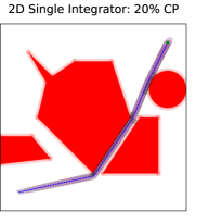
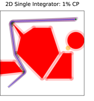
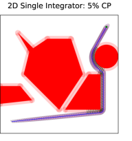
Figure 3: Illustration of the MCMP algorithm output given a range of target path CPs for a 2D single integrator system. For these uncertainty parameters, we see that the precise safety tolerance value (between 1%–20%) will correspond to a nominal solution in one of three distinct homotopy classes. The orange obstacle in (b) is added by the “block and backtrack” modification, discussed in Section 7, to the basic MCMP bisection Algorithm 2. The black and green lines denote the close obstacle points and vectors defining their half planes respectively; only the pruned set is depicted.

Figures 2 and 3 display some example results for single integrator ($\dot{x}=u$) and double integrator ($\ddot{x}=u$) systems in a two-dimensional workspace, and Table 1 summarizes a range of statistics on algorithm performance in three-dimensional workspaces as well. The deterministic planning step (Algorithm 2, line 2) was accomplished using the differential FMT${}^{*}\,$algorithm Schmerling et al. (2015) on a fixed set of nodes. By caching nearest-neighbor and distance data for these nodes (Offline Planning), the total replanning time over all inflation factors (Online Planning, essentially consisting only of collision checking) was significantly reduced. For the single integrator systems 2D SI and 3D SI, the planning problem is equivalent to geometric planning, which allowed us to apply the ADAPTIVE-SHORTCUT rubber-band-style heuristic for smoothing planned paths Hsu (2000). Applying this smoothing heuristic ensures that the path CP varies continuously with inflation factor within a path homotopy class. Between homotopy classes the CP may be discontinuous as a function of inflation factor. If increasing the inflation factor increases the CP discontinuously, the bisection process is not affected; otherwise if the CP decreases (e.g. Figure 3 (b) and (c)—the CPs are 0.3% and 1.5% respectively around the inflation factor which closes off the (c) route) the MCMP bisection algorithm may get stuck before reaching the target CP $\alpha$ (e.g. 1% in the case of Table 1 row 2). To remedy this issue, we implemented a “block and backtrack” modification to Algorithm 2 which blocks off the riskier homotopy class with an obstacle placed at its waypoint most likely to be in collision, and then resets the bisection lower bound for the inflation factor. This results in increased computation time, but returns a path with the goal CP in the end.

We did not implement any smoothing procedure for the double integrator systems. Each nominal trajectory is selected as a concatenation of local steering connections, subject to variance in the placement of the finite set of planning nodes. In practice, this means that path CP is piecewise constant, with many small discontinuities, as a function of inflation factor. If the bisection procedure terminates at an interval around the desired CP, we choose the path satisfying the safety constraint: this explains the mean True CP below the goal value in Table 1 rows 4 and 5.

In order to speed up the Monte Carlo CP estimation, we prune the set of close obstacle points $\mathbf{z}_{t}^{(i)}$ so that the ones that remain are expected to have their term in the mixture distribution $Q$ sampled at least once. We note that this style of pruning does not bias the results; it only affects computation time and estimator variance. Additionally, since during each MCMP run we only use the CP estimate for bisection, we also save time by terminating the estimation procedure early when estimated estimator variance suggests we may do so with confidence.

	Goal	Offline	Online	MC	Discretization	Bisection	MC
	CP (%)	Planning (s)	Planning (s)	Time (s)	Points	Iterations	Particles
2D SI (A)	1	0.25 $\pm$ 0.03	1.25 $\pm$ 0.24	2.64 $\pm$ 0.83	102.5 $\pm$ 0.8	6.3 $\pm$ 1.5	2085 $\pm$ 686
2D SI (B)	1	0.27 $\pm$ 0.04	2.48 $\pm$ 0.77	4.65 $\pm$ 1.70	116.5 $\pm$ 0.7	13.3 $\pm$ 4.4	2955 $\pm$ 1052
3D SI	1	0.35 $\pm$ 0.03	1.95 $\pm$ 0.76	3.00 $\pm$ 0.89	83.6 $\pm$ 1.4	6.3 $\pm$ 3.1	1667 $\pm$ 764
2D DI	1	6.64 $\pm$ 0.14	2.86 $\pm$ 0.98	5.82 $\pm$ 2.33	107.7 $\pm$ 6.0	8.6 $\pm$ 2.9	2383 $\pm$ 952
3D DI	1	20.90 $\pm$ 1.11	6.27 $\pm$ 2.40	7.45 $\pm$ 3.75	71.7 $\pm$ 10.8	7.8 $\pm$ 3.3	2117 $\pm$ 938

	Goal	Nominal	True (MC)	Additive	Multiplicative	Cond. Mult.
	CP (%)	Path Cost	CP (%)	Estimate (%)	Estimate (%)	Estimate (%)
2D SI (A)	1	1.47 $\pm$ 0.00	1.01 $\pm$ 0.06	22.67 $\pm$ 2.39	20.35 $\pm$ 1.92	2.04 $\pm$ 0.20
2D SI (B)	1	1.69 $\pm$ 0.01	1.00 $\pm$ 0.06	12.88 $\pm$ 3.72	12.10 $\pm$ 2.97	1.37 $\pm$ 0.26
3D SI	1	1.28 $\pm$ 0.03	1.00 $\pm$ 0.06	47.48 $\pm$ 7.98	38.84 $\pm$ 5.51	2.15 $\pm$ 0.23
2D DI	1	7.20 $\pm$ 0.43	0.67 $\pm$ 0.27	15.04 $\pm$ 8.97	13.78 $\pm$ 7.59	1.39 $\pm$ 0.68
3D DI	1	9.97 $\pm$ 1.61	0.66 $\pm$ 0.33	12.26 $\pm$ 5.88	11.68 $\pm$ 5.43	0.59 $\pm$ 0.32

Table 1: (MCMP in various state spaces). Results averaged over 400 MCMP runs: 20 runs each for 20 SBMP sample sets. SI and DI denote single and double integrator respectively. We aim to minimize arc-length for the SI systems, and a mixed time/control energy cost for the DI systems. 2D SI (A) refers to the obstacle set in Figure 2, and 2D SI (B) refers to the obstacle set in Figure 3.

From Table 1 we see that MCMP run times approach real time in a range of state spaces from 2–6 dimensions, on the order of 5–10 seconds total, excluding planning computation that may be cached offline. This is accomplished even at a level of tracking discretization sufficient to approximate continuous LQG. Planning time and probability estimation time are similar in magnitude, indicating that the MC portion of MCMP is not significantly holding back algorithm run time compared to a faster approximation scheme, even in this single processor implementation. Computing the Monte Carlo path simulations (MC Particles) in parallel could greatly reduce that time. We note that the few thousand simulations required in total by MCMP would not be enough to certify, using simple Monte Carlo, that a path CP is within the interval $(0.9\%,1.1\%)$ even once, which highlights the effectiveness of our proposed estimator variance reduction techniques.

As can be seen from the simulations, the accuracies of the additive, multiplicative, and conditional multiplicative approximations vary over problems and parameters, even occasionally being quite accurate. At this level of discretization, we see that the conditional multiplicative approximation scheme is within a factor of 2 of the true CP value, but may either underestimate or overestimate depending on which of approximation (A) or (B) from Section 4 has the stronger effect. This sheds light on a key difference between using MC to estimate path CP as opposed to its alternatives: MC not only gives accurate estimates, but also comes with a standard error of that estimate, effectively allowing the user to know whether or not the estimate is a good one. On the other hand, there is no certification for the various other approximations; they simply return point values with no information about how far from the truth they are. This difference is especially crucial given the overarching goal of this exercise, which is to come up with paths that are guaranteed to have a high probability of success and have low cost. The standard error estimates that come from MC can be used as a kind of certificate of accuracy that gives the user confidence in its value, while alternatives come with no such certificate.

8 Conclusion

We have presented a computationally fast method for provably-accurate pathwise collision probability estimation using variance-reduced Monte Carlo. The variance-reduction techniques employ a novel planning-specific control variate and importance distribution. This probability-estimation technique can be used as a component in a simple meta-algorithm for chance-constrained motion planning, generating low-cost paths that are not conservative with respect to a nominal path CP constraint. Simulation results confirm our theory, and demonstrate that computation can be done at speeds amenable to real-time planning.

This works leaves many avenues for further investigation, the foremost of which is parallelization. As noted earlier, a key feature of MC is that it is trivially parallelizable (which is not changed by CV or IS). As most of the computation time is spent computing likelihood ratios, which is mostly linear algebra, our technique is ideally suited for implementation on a GPU. Another future research direction is to extend this work to more general controllers and uncertainty models. Heavier-tailed distributions, compared to the Gaussian model addressed here, would require larger shifts in inflation factor to affect similar changes in path CP, making a non-conservative CP estimation procedure all the more important. Monte Carlo itself is extremely flexible to these parameters, but it remains to be seen if appropriate control variates or importance distributions can be developed to speed it up. We note that the meta-algorithm mentioned in this paper is extremely simple, and can surely be improved upon, although there was not space in this paper to investigate all such possibilities. One potential improvement is to incorporate domain knowledge to differentially inflate the constraints, or to do so in an iterative or adaptive way, similar in spirit to Ono and Williams (2008). Another improvement could be to make bisection search adaptive and to incorporate the uncertainty in the probability estimates. We also reiterate that the meta-algorithm can be used with any deterministic planning algorithm, and thus it is worth exploring which particular algorithms are best for different planning problems and cost functions. Finally, although we use our MC method to solve the chance-constrained motion planning problem, it is in no way tied to that problem, and we plan to test our method on other problems, such as minimizing CP or optimizing a objective function that penalizes CP.

A Problem Formulation

As briefly discussed in Section 3, we consider the evolution of the robot’s path as a discrete approximation of an LQG controller tracking a continuous nominal trajectory. Here we provide the complete characterization of the problem setup.

A.1 Continuous-time formulation

We assume the robot’s dynamics evolve according to the stochastic linear model:

$$\dot{\mathbf{x}}(t)=A_{c}\mathbf{x}(t)+B_{c}\mathbf{u}(t)+\mathbf{v}(t),\qquad\quad\mathbf{y}(t)=C_{c}\mathbf{x}(t)+\mathbf{w}(t),$$ (13)

where $\mathbf{x}(t)\in{\mathbb{R}}^{d}$ is the state, $\mathbf{u}(t)\in{\mathbb{R}}^{\ell}$ is the control input, $\mathbf{y}(t)$ is the observed output, and $\mathbf{v}\sim\mathcal{N}(\mathbf{0},V_{c})$ and $\mathbf{w}\sim\mathcal{N}(\mathbf{0},W_{c})$ represent Gaussian process and measurement noise, respectively. Let $\mathcal{X}_{\text{obs}}$ be the obstacle space, so that $\mbox{$\mathcal{X}_{\text{free}}$}:={\mathbb{R}}^{d}\backslash\mbox{$\mathcal{X}_{\text{obs}}$}$ is the free space. Let $\mbox{$\mathcal{X}_{\text{goal}}$}\subset\mbox{$\mathcal{X}_{\text{free}}$}$ and $\mbox{$\bm{x}_{0}$}\in\mbox{$\mathcal{X}_{\text{free}}$}$ be the goal region and initial state, respectively.

Let $\mathbf{x}^{\text{nom}}(t)$ be a nominal solution, i.e., a solution to the deterministic version of the system’s equations:

$$\dot{\mathbf{x}}^{\text{nom}}(t)=A_{c}\mathbf{x}^{\text{nom}}(t)+B_{c}\mathbf{u}^{\text{nom}}(t),\qquad\quad\mathbf{y}^{\text{nom}}(t)=C_{c}\mathbf{x}^{\text{nom}}(t),$$

where $\mathbf{u}^{\text{nom}}(t)$ is the nominal control input, $\mathbf{y}^{\text{nom}}(t)$ is the nominal measured output, $\mathbf{x}^{\text{nom}}_{0}$ is the (deterministic) initial state, $\mathbf{x}^{\text{nom}}(T)\in\mbox{$\mathcal{X}_{\text{goal}}$}$, and $T$ is the final time. Consider the deviation variables $\delta\mathbf{x}(t):=\mathbf{x}(t)-\mathbf{x}^{\text{nom}}(t)$, $\delta\mathbf{u}(t):=\mathbf{u}(t)-\mathbf{u}^{\text{nom}}(t)$, and $\delta\mathbf{y}(t):=\mathbf{y}(t)-\mathbf{y}^{\text{nom}}(t)$. The dynamics of the deviation variables are readily obtained as

$$\dot{\delta}\mathbf{x}(t)=A_{c}\delta\mathbf{x}(t)+B_{c}\delta\mathbf{u}(t)+\mathbf{v}(t),\qquad\quad\delta\mathbf{y}(t)=C_{c}\delta\mathbf{x}(t)+\mathbf{w}(t),$$

where $\delta\mathbf{x}(0)$ is the initial condition. Consider the quadratic cost functional

$$J=\mathbb{E}\left[\delta\mathbf{x}(T)^{T}F\delta\mathbf{x}(T)\!+\!\int_{0}^{T}\!\!\delta\mathbf{x}(t)^{T}Q\delta\mathbf{x}(t)\!+\!\delta\mathbf{u}(t)^{T}R\delta\mathbf{u}(t)\right].$$

The functional $J$ is minimized by the Linear Quadratic Gaussian (LQG) controller [Speyer and Chung, 2008, Chapter 9] $\delta\mathbf{u}^{\text{LQG}}(t)=L(t)\,\widehat{\delta}\mathbf{x}(t)$, where $L(t)$ is the linear quadratic regulator (LQR) state feedback gain and $\widehat{\delta}\mathbf{x}(t)$ is the Kalman filter estimate of $\delta\mathbf{x}(t)$ (we refer the reader to [Speyer and Chung, 2008, Chapter 9] for further details on the continuous formulation and provide below detailed equations for the discrete version of the problem).

We are now in a position to state the problem we wish to solve. In words, we seek to compute a nominal path of minimum cost subject to the constraint that the stochastic dynamics driven by a reference-tracking LQG controller are collision-free with high probability. More rigorously, for a given nonnegative cost function $c$ (e.g., length) acting on paths, the stochastic motion planning problem is defined as

Stochastic motion planning (SMP):

$$\begin{split}\min_{\mathbf{u}^{\text{nom}}(\cdot)}&\quad c(\mathbf{x}^{\text{nom}}(\cdot))\\ \text{s.t.}&\quad\mathbb{P}\left(\exists t:\mathbf{x}(t)\in\mbox{$\mathcal{X}_{\text{obs}}$}\right)\leq\alpha\\ &\quad\mathbf{u}(t)=\mathbf{u}^{\text{nom}}(t)+\delta\mathbf{u}^{\text{LQG}}(t)\\ &\quad\mathbf{x}(0)\sim\mathcal{N}(\mathbf{x}^{\text{nom}}_{0},P_{0}),\quad\mathbf{x}(T)\in\mbox{$\mathcal{X}_{\text{goal}}$}\\ &\quad\text{Equation \eqref{eq:cont}}\end{split}$$ (14)

A.2 Discrete Approximation

To solve the SMP problem, one is required to compute path collision probabilities $\mathbb{P}\left(\exists t:\mathbf{x}(t)\in\mbox{$\mathcal{X}_{\text{obs}}$}\right)$. To make the problem tractable, we consider a discrete formulation whereby the dynamics are given by

$$\mathbf{x}_{t+1}=A\mathbf{x}_{t}+B\mathbf{u}_{t}+\mathbf{v}_{t},\quad\mathbf{v}_{t}\sim\mathcal{N}(\mathbf{0},V),\quad\mathbf{y}_{t}=C\mathbf{x}_{t}+\mathbf{w}_{t},\quad\mathbf{w}_{t}\sim\mathcal{N}(\mathbf{0},W),$$ (15)

for a given fixed timestep ${\Delta t}$. In equation (15), we used the definitions

$$A:=e^{A_{c}{\Delta t}},\quad B:=\left(\int_{0}^{\Delta t}e^{A_{c}s}ds\right)B_{c},\quad C:=C_{c},\quad V:=\int_{0}^{\Delta t}e^{A_{c}s}V_{c}e^{A^{T}_{c}s}ds,\quad W:=\frac{1}{{\Delta t}}W_{c}.$$

The deviation variables are then defined as $\delta\mathbf{x}_{t}:=\mathbf{x}_{t}-\mathbf{x}^{\text{nom}}_{t}$, $\delta\mathbf{u}_{t}:=\mathbf{u}_{t}-\mathbf{u}^{\text{nom}}_{t}$, and $\delta\mathbf{y}_{t}:=\mathbf{y}_{t}-\mathbf{y}^{\text{nom}}_{t}$, for $t=0,\dots,T$. The cost function for the discrete LQG controller is given by

$$J=\mathbb{E}\left[\delta\mathbf{x}_{T}^{T}F\delta\mathbf{x}_{T}+\sum_{t=0}^{T-1}\delta\mathbf{x}_{t}^{T}Q\delta\mathbf{x}_{t}+\delta\mathbf{u}_{t}^{T}R\delta\mathbf{u}_{t}\right],$$

and the LQG controller minimizing $J$ is given in Shaiju and Petersen [2008] by $\delta\mathbf{u}^{\text{LQG}}_{t}=L_{t}\,\widehat{\delta}\mathbf{x}_{t}$, where the feedback gain is

$$L_{t} =-(R+B^{T}S_{t+1}B)^{-1}B^{T}S_{t+1}A,$$

$$S_{t} =Q+A^{T}\left(S_{t+1}-S_{t+1}B(R+B^{T}S_{t+1}B)^{-1}B^{T}S_{t+1}\right)A,\qquad S_{T}=F,$$

and the Kalman estimate dynamics are

$$\widehat{\delta}\mathbf{x}_{t+1}=A\widehat{\delta}\mathbf{x}_{t}+BL_{t}\widehat{\delta}\mathbf{x}_{t}+K_{t}(\delta\mathbf{y}-C\widehat{\delta}\mathbf{x}_{t}),$$

$$K_{t}=AP_{t}C^{T}(W+CP_{t}C)^{-1},\qquad P_{t+1}=V+A\left(P_{t}-P_{t}C^{T}(W+CP_{t}C)^{-1}CP_{t}\right)A^{T},$$

with $P_{0}$ denoting the covariance of the initial state $\mathbf{x}_{0}$ (and hence of $\delta\mathbf{x}_{0}$). The combined system evolves according to

$$\begin{bmatrix}\delta\mathbf{x}_{t+1}\\ \widehat{\delta}\mathbf{x}_{t+1}\end{bmatrix}=\begin{bmatrix}A&BL_{t}\\ K_{t}C&A+BL_{t}-K_{t}C\end{bmatrix}\begin{bmatrix}\delta\mathbf{x}_{t}\\ \widehat{\delta}\mathbf{x}_{t}\end{bmatrix}+\begin{bmatrix}\mathbf{v}_{t}\\ K_{t}\mathbf{w}_{t}\end{bmatrix}=M_{t}\begin{bmatrix}\delta\mathbf{x}_{t}\\ \widehat{\delta}\mathbf{x}_{t}\end{bmatrix}+\mathbf{n}_{t},$$ (16)

where $\mathbf{n}_{t}\sim\mathcal{N}\left(\mathbf{0},N_{t}=\begin{bmatrix}V&0\\ 0&K_{t}WK_{t}^{T}\end{bmatrix}\right)$. Equation (16), in addition to providing a formula for simulating state trajectories, also represents a means for tracking the state uncertainty at each time step. Given that $\begin{bmatrix}\delta\mathbf{x}_{t}\\ \widehat{\delta}\mathbf{x}_{t}\end{bmatrix}\sim\mathcal{N}\left(\mu_{t},\Sigma_{t}\right)$, we have that

$$\begin{bmatrix}\delta\mathbf{x}_{t+1}\\ \widehat{\delta}\mathbf{x}_{t+1}\end{bmatrix}\sim\mathcal{N}\left(\mu_{t+1}=M_{t}\mu_{t},\Sigma_{t+1}=M_{t}\Sigma_{t}M_{t}^{T}+N_{t}\right).$$ (17)

Using this recursion we may compute the marginal distributions of each waypoint along the full LQG-controlled trajectory, starting from $\mu_{0}=\mathbf{0}$ and $\Sigma_{0}=\begin{bmatrix}P_{0}&0\\ 0&0\end{bmatrix}$. Letting $\overline{\mathbf{x}_{0},\dots,\mathbf{x}_{T}}$ denote the continuous curve traced by the robot’s random trajectory (which connects the points $\mathbf{x}_{0},\dots,\mathbf{x}_{T}$), the problem we wish to solve then becomes:

Discretized SMP:

$$\begin{split}\min_{\mathbf{u}^{\text{nom}}(\cdot)}&\quad c(\mathbf{x}^{\text{nom}}(\cdot))\\ \text{s.t.}&\quad\mathbb{P}\left(\overline{\mathbf{x}_{0},\dots,\mathbf{x}_{T}}\cap\mbox{$\mathcal{X}_{\text{obs}}$}\neq\varnothing\right)\leq\alpha\\ &\quad\mathbf{u}_{t}=\mathbf{u}^{\text{nom}}_{t}+\delta\mathbf{u}^{\text{LQG}}_{t}\\ &\quad\mathbf{x}_{0}\sim\mathcal{N}(\mathbf{x}^{\text{nom}}_{0},P_{0}),\quad\mathbf{x}_{T}\in\mbox{$\mathcal{X}_{\text{goal}}$}\\ &\quad\text{Equation \eqref{eqn:APP_DLQG}}\end{split}$$ (18)

References

- Aoude et al. [2013] G. S. Aoude, B. D. Luders, J. M. Joseph, N. Roy, and J. P. How. Probabilistically safe motion planning to avoid dynamic obstacles with uncertain motion patterns. Autonomous Robots, 35(1):51–76, 2013.
- Berg et al. [2011] J. V. D. Berg, P. Abbeel, and K. Goldberg. LQG-MP: Optimized path planning for robots with motion uncertainty and imperfect state information. International Journal of Robotics Research, 30(7):895–913, 2011.
- Bezanson et al. [2012] J. Bezanson, S. Karpinski, V. B. Shah, and A. Edelman. Julia: A fast dynamic language for technical computing. 2012. Available at http://arxiv.org/abs/1209.5145.
- Blackmore et al. [2010] L. Blackmore, M. Ono, A. Bektassov, and B. C. Williams. A probabilistic particle-control approximation of chance-constrained stochastic predictive control. IEEE Transactions on Robotics, 26(3):502–517, 2010.
- Hsu [2000] D. Hsu. Randomized Single-Query Motion Planning in Expansive Spaces. PhD thesis, Stanford University, 2000.
- Janson et al. [2015] L. Janson, E. Schmerling, and M. Pavone. Monte Carlo motion planning for robot trajectory optimization under uncertainty (extended version). Available at http://web.stanford.edu/~pavone/papers/JSP.ISRR15.pdf, 2015.
- Kaelbling et al. [1998] L. P. Kaelbling, M. L. Littman, and A.R. Cassandra. Planning and acting in partially observable stochastic domains. Artificial Intelligence, 101(1-2):99–134, 1998.
- Kothari and Postlethwaite [2013] M. Kothari and I. Postlethwaite. A probabilistically robust path planning algorithm for uavs using rapidly-exploring random trees. Journal of Intelligent & Robotic Systems, 71(2):231–253, 2013.
- Kurniawati et al. [2008] H. Kurniawati, D. Hsu, and W. S. Lee. SARSOP: Efficient point-based POMDP planning by approximating optimally reachable belief spaces. In Robotics: Science and Systems, pages 65–72, 2008.
- LaValle [2006] S. M. LaValle. Planning Algorithms. Cambridge University Press, 2006.
- LaValle [2011] S. M. LaValle. Motion planning: Wild frontiers. IEEE Robotics Automation Magazine, 18(2):108–118, 2011.
- LaValle and Kuffner [2001] S. M. LaValle and J. J. Kuffner. Randomized kinodynamic planning. International Journal of Robotics Research, 20(5):378–400, 2001.
- Liu and Ang [2014] W. Liu and M. H. Ang. Incremental sampling-based algorithm for risk-aware planning under motion uncertainty. In Proc. IEEE Conf. on Robotics and Automation, pages 2051–2058, May 2014.
- Luders et al. [2010] B. Luders, M. Kothari, and J. P. How. Chance constrained RRT for probabilistic robustness to environmental uncertainty. In AIAA Conf. on Guidance, Navigation and Control, 2010.
- Luders et al. [2013a] B. D. Luders, S. Karaman, and J. P. How. Robust sampling-based motion planning with asymptotic optimality guarantees. In AIAA Conf. on Guidance, Navigation and Control, 2013a.
- Luders et al. [2013b] B. D. Luders, I. Sugel, and J. P. How. Robust trajectory planning for autonomous parafoils under wind uncertainty. In AIAA Conf. on Guidance, Navigation and Control, 2013b.
- Oldewurtel et al. [2008] F. Oldewurtel, C. Jones, and M. Morari. A tractable approximation of chance constrained stochastic mpc based on affine disturbance feedback. In Proc. IEEE Conf. on Decision and Control, pages 4731–4736, 2008.
- Ono and Williams [2008] M. Ono and B.C. Williams. Iterative risk allocation: A new approach to robust model predictive control with a joint chance constraint. In Decision and Control, 2008. CDC 2008. 47th IEEE Conference on, pages 3427–3432, Dec 2008. doi: 10.1109/CDC.2008.4739221.
- Ono et al. [2013] M. Ono, B. C. Williams, and L. Blackmore. Probabilistic planning for continuous dynamic systems under bounded risk. Journal of Artificial Intelligence Research, 46:511–577, 2013.
- Owen [2013] A. B. Owen. Monte Carlo theory, methods and examples. 2013. Available at http://statweb.stanford.edu/~owen/mc/.
- Patil et al. [2012] S. Patil, J. van den Berg, and R. Alterovitz. Estimating probability of collision for safe motion planning under Gaussian motion and sensing uncertainty. In Proc. IEEE Conf. on Robotics and Automation, pages 3238–3244, 2012.
- Reif [1979] J. H. Reif. Complexity of the mover’s problem and generalizations. In 20th Annual IEEE Symposium on Foundations of Computer Science, pages 421–427, San Juan, Puerto Rico, October 1979.
- Schmerling et al. [2015] E. Schmerling, L. Janson, and M. Pavone. Optimal sampling-based motion planning under differential constraints: the drift case with linear affine dynamics. Available at http://arxiv.org/abs/1405.7421/, 2015.
- Shaiju and Petersen [2008] A. J. Shaiju and I. R. Petersen. Formulas for discrete time LQR, LQG, LEQG and minimax LQG optimal control problems. In IFAC World Congress, 2008.
- Speyer and Chung [2008] J. L. Speyer and W. H. Chung. Stochastic processes, estimation, and control, volume 17. SIAM, 2008.
- Sun et al. [2013] W. Sun, L. G Torres, J. V. D. Berg, and R. Alterovitz. Safe motion planning for imprecise robotic manipulators by minimizing probability of collision. In International Symposium on Robotics Research, 2013.
- Sun et al. [2015] W. Sun, S. Patil, and R. Alterovitz. High-frequency replanning under uncertainty using parallel sampling-based motion planning. Robotics, IEEE Transactions on, 31(1):104–116, 2015.
- Thrun et al. [2001] S. Thrun, D. Fox, W. Burgard, and F. Dellaert. Robust Monte Carlo localization for mobile robots. Artificial Intelligence, 128(1-2):99–141, 2001.
- Vitus and Tomlin [2011] M. P. Vitus and C. J. Tomlin. On feedback design and risk allocation in chance constrained control. In Proc. IEEE Conf. on Decision and Control, pages 734–739, 2011.