Don’t let Google know I’m lonely

Abstract

From buying books to finding the perfect partner, we share our most intimate wants and needs with our favourite online systems. But how far should we accept promises of privacy in the face of personalised profiling? In particular, we ask how can we improve detection of sensitive topic profiling by online systems? We propose a definition of privacy disclosure we call $\epsilon$-indistinguishability from which we construct scalable, practical tools to assess learning potential from personalised content. We demonstrate our results using openly available resources, detecting a learning rate in excess of $98\%$ for a range of sensitive topics during our experiments.

¡ccs2012¿ ¡concept¿ ¡concept_id¿10002951.10003260.10003261.10003263¡/concept_id¿ ¡concept_desc¿Information systems Web search engines¡/concept_desc¿ ¡concept_significance¿500¡/concept_significance¿ ¡/concept¿ ¡concept¿ ¡concept_id¿10002951.10003260.10003261.10003271¡/concept_id¿ ¡concept_desc¿Information systems Personalization¡/concept_desc¿ ¡concept_significance¿500¡/concept_significance¿ ¡/concept¿ ¡concept¿ ¡concept_id¿10002951.10003260.10003272¡/concept_id¿ ¡concept_desc¿Information systems Online advertising¡/concept_desc¿ ¡concept_significance¿500¡/concept_significance¿ ¡/concept¿ ¡concept¿ ¡concept_id¿10002951.10003260.10003261.10003270¡/concept_id¿ ¡concept_desc¿Information systems Social recommendation¡/concept_desc¿ ¡concept_significance¿300¡/concept_significance¿ ¡/concept¿ ¡concept¿ ¡concept_id¿10002951.10003260.10003277¡/concept_id¿ ¡concept_desc¿Information systems Web mining¡/concept_desc¿ ¡concept_significance¿300¡/concept_significance¿ ¡/concept¿ ¡concept¿ ¡concept_id¿10002951.10003260.10003261.10003269¡/concept_id¿ ¡concept_desc¿Information systems Collaborative filtering¡/concept_desc¿ ¡concept_significance¿100¡/concept_significance¿ ¡/concept¿ ¡concept¿ ¡concept_id¿10002978.10003022.10003028¡/concept_id¿ ¡concept_desc¿Security and privacy Domain-specific security and privacy architectures¡/concept_desc¿ ¡concept_significance¿500¡/concept_significance¿ ¡/concept¿ ¡concept¿ ¡concept_id¿10002978.10003029.10011150¡/concept_id¿ ¡concept_desc¿Security and privacy Privacy protections¡/concept_desc¿ ¡concept_significance¿500¡/concept_significance¿ ¡/concept¿ ¡concept¿ ¡concept_id¿10002978.10003029.10011703¡/concept_id¿ ¡concept_desc¿Security and privacy Usability in security and privacy¡/concept_desc¿ ¡concept_significance¿500¡/concept_significance¿ ¡/concept¿ ¡concept¿ ¡concept_id¿10002978.10003022.10003026¡/concept_id¿ ¡concept_desc¿Security and privacy Web application security¡/concept_desc¿ ¡concept_significance¿300¡/concept_significance¿ ¡/concept¿ ¡concept¿ ¡concept_id¿10002978.10003022.10003027¡/concept_id¿ ¡concept_desc¿Security and privacy Social network security and privacy¡/concept_desc¿ ¡concept_significance¿300¡/concept_significance¿ ¡/concept¿ ¡concept¿ ¡concept_id¿10002978.10002997.10003000¡/concept_id¿ ¡concept_desc¿Security and privacy Social engineering attacks¡/concept_desc¿ ¡concept_significance¿100¡/concept_significance¿ ¡/concept¿ ¡concept¿ ¡concept_id¿10002950.10003648.10003688.10003699¡/concept_id¿ ¡concept_desc¿Mathematics of computing Exploratory data analysis¡/concept_desc¿ ¡concept_significance¿300¡/concept_significance¿ ¡/concept¿ ¡/ccs2012¿

[500]Information systems Web search engines [500]Information systems Personalization [500]Information systems Online advertising [300]Information systems Social recommendation [300]Information systems Web mining [100]Information systems Collaborative filtering [500]Security and privacy Domain-specific security and privacy architectures [500]Security and privacy Privacy protections [500]Security and privacy Usability in security and privacy [300]Security and privacy Web application security [300]Security and privacy Social network security and privacy [100]Security and privacy Social engineering attacks [300]Mathematics of computing Exploratory data analysis

Pòl Mac Aonghusa and Douglas J. Leith, 2015. Don’t let Google know I’m lonely!

Supported by Science Foundation Ireland grant 11/PI/11771.

Author’s addresses: P. Mac Aonghusa, IBM Research, IBM Technology Campus, Dublin, Ireland; Douglas J. Leith, School of Computer Science and Statistics, Trinity College Dublin, Ireland.

acmcopyright 1094-9224/2015 0000001.0000001

X 0 0 2016 05

1 Introduction

We investigate threats to user privacy due to inference by a search engine through users’ online behaviour. Of particular interest is learning related to potentially sensitive topics such as health, finance and sexual orientation. Our goal is to inform the user by detecting evidence of privacy disclosure through analysis of personalised content. Our method is readily implementable with available open tools, simple to apply, and provides highly accurate results.

Our approach is borrowed from black-box testing: given a sequence of user queries we embed a subsequence of probe queries and observe corresponding search engine responses. By analysing changes in the responses to the probe queries over time, we hope to be able to spot learning of topics the user considers sensitive and so would prefer not to disclose to the search engine.

Using Bing and Google Search, we demonstrate that by monitoring changes in the adverts displayed in the response to probe queries we are able to accurately detect evidence of learning for a range of sensitive topics in over $98\%$ of cases. Topics studied include medical conditions (cancer, anorexia etc), sexual orientation, disability, bankruptcy and unemployment. Our method is accurate, with typical false detection rates of less than $10\%$ (and less than $1\%$ for many sensitive topics). We also show that detection rates remain high for anonymous users, suggesting that search engines learn quickly; even without search history as background knowledge. Our estimation of search engine adaptation rates indicate that sensitive topic learning is detectable after as few as $3-4$ queries on average.

The main contributions in this paper are:

• A definition of privacy we call $\epsilon$-indistinguishability that is both compatible with existing privacy models and readily implementable as a practical user technology

• An effective method for change detection across a sequence of queries by collecting and comparing responses to a subsequence of preselected probe queries

• A fast, scalable estimator of $\epsilon$-indistinguishability, we call PRI (”PRivacy for Individuals”) and which we implement using standard tools and apply in subsequent experiments

• An extensive measurement campaign showing that evidence of adaptation is easy to detect for a wide range of sensitive topics.

In this paper we focus on raising awareness of privacy concerns arising from personalisation by online services. We position our contribution as a starting point in a multi-step program. Our goal here is to demonstrate that practical individual awareness is possible, providing a stepping stone toward effective counter-measures.

2 Related Work

Personalisation of web search through implicit data collection – for example location, IP address and browser agent – is well studied. See [Spiliopoulou et al. (2012)] for an historical survey of results in web mining for personalisation. Even so-called ‘private’ browsing mode may not suffice; in [Aggarwal et al. (2010)], the authors investigate how a range of popular browser extensions and plugins undermine the security of private browsing.

In [boyd (2011)], individual user concerns with privacy are viewed in terms of two major factors – awareness of a sensitive social situation, and, the ability of an individual to control the social situation. In this paper we focus on raising awareness through detection of profiling of sensitive topics. Effective counter measures allowing a user to control their exposure to profiling are outside the scope of this present paper. Evidence that users are sensitive to personalisation – and will respond to increased awareness – is given in [Panjwani et al. (2013)], where a user study of internet search users showed a slight preference for personalised content. After raising awareness by fully informing users about risks to their privacy, the majority of users were satisfied to forego personalisation when search topics were judged sensitive. In [Agarwal et al. (2013)], a larger user study explores privacy concerns in more depth, finding that users are more concerned about the potential of being shown suggestive or embarrassing content than they are of tracking.

While improved user experience is generally offered as a positive motivation for user profiling, for example, see the Google online privacy policy [Foundation (2015b)], negative associations have been reported in the research literature:

Discrimination

Negative consequences associated with personalisation are investigated in [Sweeney (2013)], where an extensive review of adverts from Google and Reuters.com showed a strong correlation between adverts suggestive of an arrest record and an individual’s ethnicity. Searches containing first names considered black-identifying were on average $25\%$ more likely to receive adverts indicative of an arrest record than searches including white-identifying first names. In [Guha et al. (2010)], the authors identified more than half of online advertising targeted exclusively to gay men was neutral to sexual-orientation – posing a privacy threat through inadvertant user clicking. Our experiments confirm that evidence of profiling that could be termed discriminatory is detectable with high confidence.

Censorship

Personalisation as a form of censorship – termed a filter bubble in [Pariser (2011)] – is explored in [Hannak et al. (2013)]. In a filter bubble, a user cannot access subsets of information because the recommender system algorithm has decided it is irrelevant for that user. In [Hannak et al. (2013)] a filter bubble effect was detected in the case of Google Web Search in a test using 200 users. Censorship is an interesting complimentary perspective on user profiling that is not considered in this paper.

Much of the research literature in recommender system privacy has focused on techniques to implement privacy; for data processing on the server side – or – on the user side, techniques to obfuscate, encrypt or otherwise hide queries or mask user identity from the recommender. The query masking or obfuscation technique has been explored extensively, see for example [Howe et al. (2009), Peddinti and Saxena (2011)]. The essential challenge in this type of approach is to define a practical method of selecting the ‘noise’ queries and clicks to provide a verifiable level of anonymity while not overly upsetting overall utility. In our experiments we observe the recommender systems responding quickly to changes in user topic, compensating quickly after topic changes so that ‘noise injection’ alone may not provide adequate protection.

Several authors have examined privacy in the context of recommender systems, broadly addressing the question of data privacy with respect to the user data once collected by the recommender. In a 2001 work, [Ramakrishnan et al. (2001)], the authors identify threats from data linking or combination by identifying similar patterns of preference or behaviour conjunction with other data sources to uncover identities and reveal personal details. In their concluding remarks, the authors state that “the ideal deterrents are better awareness of the issues and more openness in how systems operate in the marketplace. In particular, individual sites should clearly state the policies and methodologies they employ with recommender systems”.

Techniques for preserving individual user privacy or anonymity have also been extensively discussed in the literature. A typical approach is to apply encryption and multi-party computation techniques to process sensitive user queries, leveraging techniques from the privacy preserving data mining domain. For example, in [Erkin et al. (2010), Erkin et al. (2011)], the authors propose to encrypt privacy sensitive data and generate recommendations by processing them under encryption. Approaches of this type typically rely on a user, or a learning algorithm, being able to identify which queries are sensitive, and trust in the service provider to perform query processing under secure encryption. In contrast, our approach seeks to inform a user about their ongoing privacy status.

Accountability, and enforcement of accountability, for privacy policy is an active area of research. Regulatory requirements for data handling in industries such as Healthcare (HIPPA) and Finance (GLBA) are well established. The position with respect to handling of data collected by online recommender systems is less clear. In [Datta (2014)], the author reviews computational approaches to specification and enforcement of privacy policies at large scale. Our approach differs in design, being intended for individual user implementation. While we also make use of inference, it is statistical inference rather than the logic-based inference approach discussed in [Datta (2014)].

Tools that seek to inform a user about whether an adversary is potentially gathering and sharing information exist. Browser add-ons such as Mozilla Lightbeam, [Foundation (2015c)], and PrivacyBadger, [Foundation (2015a)], show a user where data is shared with third parties from sites they visit. XRay, [Lécuyer et al. (2014)], reports high accuracy in identifying which sources of user data such as email or web search history might have triggered particular results from online services such as adverts.

Privad, [Guha et al. (2011)], and ObliviAd, [Backes et al. (2012)] allow advertisers to provide private advertising, by employing intermediate agents to mask direct access to user information. In both cases external agents hide user intentions and interactions with adverts. ObliviAd use secure hardware-based private information retrieval for advert distribution, with advertiser billing provided by secure tokens. These features allow the authors to provide provable cryptographic guarantees of anonymity for users of the system.

The importance of adverts to commercial search engines is underlined by the volume of research into how to position adverts to direct user attention to them. The position of commercial content on a result page is a key determinant of whether an advert will be selected or not. For example, in [Jansen et al. (2013)], the authors determined that the first advert on a page accounts for approximately $80\%$ of commercial revenue. In [Richardson et al. (2007)], the authors include results from user eye-tracking demonstrating how dramatically a user focuses on the first few results on a page.

Recommender systems continue to evolve more sophisticated methods of content selection. Semantic targetting techniques, where the overall theme of a web-page is used to select contextually related adverts, are used by companies such as Google Knowledge Graph, [Graph (2015)], and iSense, [iSense (2015)], while Zemanta, [Zemanta (2015)], provides a browser add-on that suggests semantically relevant articles, images, links and keywords to content creators. Experimental results, with Google in particular, appear to show early promise that the PRI technique applies to content selection models other than keyword-based .

Modelling a system as a black-box, where internal details of recommender systems algorithms and settings are unknown to users, is mentioned in several sources [Datta (2014)] and [Hannak et al. (2013)]. While the term “black-box” is used extensively throughout the privacy literature, the present authors have not seen black-box testing techniques – such as employing probes to calibrate responses – using extensively in the privacy literature.

In this paper, we seek a practical approach, allowing a user inform themselves of privacy disclosure threats due to search engine inference. By exploiting the idea that a commercial search engine combines user data with background knowledge to create personalised recommendations we ask how to assess ongoing risks to privacy based on simple observation of the recommender? In this way we help a user to make reasonable assessments of the ongoing risk of disclosure while using a search engine.

3 Threat Model

We consider privacy for a class of commercial internet systems seeking to maximise expected revenue by personalising commercial content to attract user interest. Users are generally aware of good privacy practice for obviously personally identifying information – such as name, address and credit card numbers – reflecting the visibility of personal identifiability as a central concept in information privacy regulation [Schwartz and Solove (2011), Ohm (2010)]. Personalisation practices, based on obvious features such as location, IP address and browser identifier, are also well known and extensively discussed in the literature [Spiliopoulou et al. (2012)]. In this paper we focus on detecting evidence of recommender system learning. User traceability or pseudo-anonymity is not considered.

It seems reasonable to assume that a for-profit commercial search engine selects page content to maximise its expected revenue. This means that when a search engine infers that a particular advertising topic is likely to be of interest to a user, and so more likely to generate click through and sales, it is obliged to use this information when selecting which adverts to display.

In this context the threat model we consider is one of distinguishability rather than individual identifiability – a search engine does not seek to identify the user as an individual but rather it seeks to determine the user’s likely interest in commercially valuable topics. Privacy becomes an issue when any of the topics matches subjects deemed sensitive by the user.

Since a revenue maximising search engine acts to display adverts associated with topics it detects are most interesting to the user, the potential exists to detect search engine learning via analysis of changes in the choice of displayed adverts and to inform the user of this learning.

In our experiments we find that adverts do indeed provide sufficiently dynamic content, as we shall show in Section 5.6. We note that, over the period of short query sessions we consider here, page content is usually constrained to be relatively insensitive with respect to personalisation in order to provide so-called rank-stability; link-based search algorithms are termed rank-stable if small perturbations in the link structure of the input graph do not affect the output ranking order it produces, [Lempel and Moran (2005)] and [Langville and Meyer (2006)]. In contrast, adverts may be chosen relatively freely, a fact which has also been noted by other authors, for example see [Guha et al. (2010)].

Evidence that page content varies for individuals over periods of time has been reported. [Hannak et al. (2013)] also observes that localised content such as news items is necessarily volatile and will vary to reflect currency. Our focus, in this paper, is on detecting learning by observing adverts and we do not consider other personalised content such as news and weather specifically in this study. For the typical period of time of a typical user session in this study – typically less than 20 minutes – experimental results in Section 5.6 indicate the assumption of “short-term” rank-stability in page content considered in our study is reasonable.

4 Mathematical Formulation

4.1 $\epsilon$-indistinguishability

We assume that a user interacts with a search engine by issuing a query, receiving a web page in response and then clicking on one or more items in the response. A single such interaction, labeled with index $j$, consists of a query, response page, item-click triple, denoted $\Omega_{j}=\left(q_{j},p_{j},l_{j}\right)$. A user session of length $k>0$ steps consists of a sequence of $k$ individual steps, and is denoted $\left\{\Omega_{k}\right\}_{k\geq 1}$. The sequence of interactions $\left\{\Omega_{k}\right\}_{k\geq 1}$ is jointly observed by the user and the search engine – and perhaps several other third-party observers.

Let $\mathscr{E}_{k}$ denote the prior evidence – also referred to as background knowledge – available to an observer at the start of step $k$. We assume the search engine does not change its background knowledge during a user session other than through $\Omega_{k}$. That is, $\mathscr{E}_{1}$ denotes the prior evidence available to an observer before the user session begins, e.g. the user’s login profile, historical queries, weblogs etc, and for $k=2,3,\cdots$ we have,

$$\mathscr{E}_{k} =\{\mathscr{E}_{k-1},\Omega_{k-1}\}$$

Let $C=\{c_{1},\ldots,c_{N}\}$ denote a set of interest categories which the user considers to be sensitive, e.g. bankrupt, cancer, addiction, etc and gather all non-sensitive interest categories into a catch-all category denoted $\bar{c}$. The category in which the user is interested in the current session is a random variable $X_{c}$ taking values in $C\cup\{\bar{c}\}$. In subsequent experiments multiple sensitive user categories will sometimes be aggregated into a single sensitive topic for clarity, so that $C\cup\{\bar{c}\}=${sensitive, non-sensitive} in this simplified case. The term “category” here denotes a topic or theme of interest to the user. Since the search engine adversary is regarded as a black-box we do not know if such user categories correspond to internal classifications by the adversary. Our intent is to detect if there is evidence of learning about user categories of interest to the user. We do not attempt to understand what internal classifications – if any – the search engine might apply to the user.

We adopt an indistinguishability definition of disclosure risk, tailored to our particular context:

Definition 4.1 ( $\epsilon$-indistinguishability ).

A user session $\Omega_{k}$ satisfies $\epsilon$-indistinguishability with respect to sensitive category $c\in C$ if there exists an $\epsilon>0$ such that

$$M_{k}(c)\leq e^{\epsilon},\ \ k=1,2,\cdots$$ (1)

where

$$M_{k}(c):=\frac{\text{\rm Prob}(X_{c}=c|\Omega_{k},\mathscr{E}_{k})}{\text{\rm Prob}(X_{c}=c|\mathscr{E}_{1})}$$ (2)

In other words there is a posteriori indistinguishability of interest in sensitive category $c$ after observing $\Omega_{k}$, $k=1,2,\cdots$.

Given the sequence of observations $\{\Omega_{k}\}_{k\geq 1}$ our aim is, with high probability, to (1) determine whether $\epsilon$-indistinguishability has been violated for one or more of the sensitive categories in $C$ (and so the adversary is likely to have successfully learned about the users interest in one or more of these categories), and (2) identify which of these sensitive categories have been learned.

4.2 Using Probe Queries to Simplify Estimation

Estimating $M_{k}(c)$ is challenging since it depends on the full user session history $\{\Omega_{j}\}_{j=1,\dots,k}$ up to step $k$. To simplify the task we assume that the user issues a pre-defined probe query at intervals during the session and that the links in the response to this query are not clicked. In brief, a probe query should be plausible in relation to a sensitive topic so that it does not suggest a change of topic to the search engine; a probe query should also be ambiguous so that the search engine has several possible adaptations to the probe query. In Section 5.3 experimental probe query selection is discussed, where selecting high-frequency terms appearing on multiple search result pages, while taking care to avoid obviously revealing terms, is shown to be a practical method of probe selection. In practice, a probe query might be issued in an automated manner by the user’s browser and the response processed in the background so as not to disturb the user.

In addition, we make the following assumptions.

Assumption 1 (Informative Probe Query).

Let $K\subset\{1,2,\cdots\}$ label the subsequence of steps at which a probe query is issued. At each step $k\in K$ at which a probe query is issued,

$$\frac{\text{\rm Prob}(X_{c}=c|\Omega_{k},\mathscr{E}_{k})}{\text{\rm Prob}(X_{c}=c|\mathscr{E}_{1})} =\frac{\text{\rm Prob}(X_{c}=c|\Omega_{k},\mathscr{E}_{1})}{\text{\rm Prob}(X_{c}=c|\mathscr{E}_{1})}$$ (3)

That is, it is not necessary to explicitly use knowledge of the search history during the current session when estimating $M_{k}(c)$ as this is already reflected in the response to the probe query at step $k$. Assumption 1 greatly simplifies estimation as it means we do not have to take account of the full search history, but requires that the response to the probe query reveals any search engine learning of interest in sensitive category $c$ which has occurred. Methods for the selection of an appropriate probe query that tends to elicit revealing responses are discussed in detail in Section 5.3.

Assumption 2 (Revealing Adverts).

In the search engine response to the probe query at step $k$ it is the adverts ${a}_{k}$ on response page $p_{k}$ which primarily reveal learning of sensitive categories. Therefore, since the probe query is fixed and the response page – for probe queries – is not clicked by the user,

$$\text{\rm Prob}(X_{c}=c|\Omega_{k},\mathscr{E}_{1})=\text{\rm Prob}(X_{c}=c|{a}_{k},\mathscr{E}_{1}),\ k\in K$$ (4)

This is in line with the observation in Section 3 that, over the lifetime of a typical user session, the informational response (search result links etc) to a query tends to be insensitive to learning of user interests. Note that personalisation of search results over longer time scales e.g. in response to changes in geographic location may still occur.

Under Assumptions 1-2, when

$${M}_{k}(c)=\frac{\text{\rm Prob}(X_{c}=c|{a}_{k},\mathscr{E}_{1})}{\text{\rm Prob}(X_{c}=c|\mathscr{E}_{1})}>e^{\epsilon}$$ (5)

for any $k\in K$ then $\epsilon$-indistinguishability is violated. To ensure that the converse holds, namely that when ${M}_{k}(c)\leq e^{\epsilon}$ for all $k\in K$ then $\epsilon$-indistinguishability is satisfied, we also need the following assumption.

Assumption 3 (Sufficiency of Sampling).

When $M_{k}(c)\leq e^{\epsilon}$ for $k\in K$ then $M_{k}(c)\leq e^{\epsilon}$ for $k\in\{1,2,\cdots\}$. That is, when $\epsilon$-indistinguishability is satisfied at the subsequence of steps $K$ at which the probe query is issued then it is satisfied at all steps.

In practice it can be difficult to verify whether Assumption 3 holds or not. When we cannot rely on Assumption 3 then, as already noted, violations ${M}_{k}(c)>e^{\epsilon}$ for $k\in K$ are still informative of disclosure risk and analysis based on the values ${M}_{k}(c)$, $k\in K$ should be regarded as an underestimate, or lower bound, of disclosure risk for the user.

4.3 Advert Text Processing

We briefly summarise Natural Language Processing (NLP) techniques we use to preprocess advert text into a format for analysis. For a full treatment of these techniques, using the Python language, see [Bird et al. (2009)].

In the first preprocessing step, advert text from result pages is extracted and tokenised into individual words by using white-spaces and punctuation as token separators. Common, uninformative high-frequency stop-words are removed and stemming is performed to remove common prefixes and suffixes, for example, $\{\text{clicking, clicks, clicked}\}\rightarrow\{\text{click}\}$ . After preprocessing and during the training phase we assign each unique keyword an integer id and also count the keyword’s frequency of occurrence in the training set to produce a lookup table of keyword id-frequency pairs. The lookup table of keywords and associated occurence counts is generally termed a Term-Frequency (TF) representation in NLP. Because the previous preprocessing step has removed uninformative high frequency words and has reduced word variations through stemming, the TF table transforms advert text to a smaller more computable representation.

During subsequent testing, an advert encountered on a result page is first preprocessed and then mapped to keyword ids the TF table. Preprocessing an advert in this way is called vectorisation in NLP, where the $\text{n}^{th}$ component of the vectorised advert is the number of occurences in the advert of the keyword stem with integer id n. Given two vectorised adverts it is now possible, for example, to compute similarity measures between adverts using any convenient vector metric – such as Cosine Similarity which is effectively vector inner product.

To streamline notation we assume that the available advert locations are the same for all pages $p_{k}$, $k=1,2,\cdots$. Let ${a}_{k}=\{a_{1,k},\cdots,a_{n,k}\}$ be the set of adverts on page $p_{k}$. An advert $a_{i,k}=\{w_{1},w_{2},\cdots,w_{|a_{i,k}|}\}$ appearing on a result page is modelled as a sequence of words drawn from a set of natural language terms $D$ (as discussed later, in our work we derive this set from training data). In practice result pages may contain localised content, such as news and weather, as well as other format content such as images and links, but leave consideration of these to future work.

We represent text preprocessing operations such as stemming and stop word removal operations as a filter over $D$. Specifically, let $f:D\rightarrow\tilde{D}\cup\emptyset$ be a text processing/filtering map taking words in dictionary $D$ either to a content-bearing term in set $\tilde{D}$ or to a null term $\emptyset$ corresponding to deletion of the word. Let $\tilde{a}_{i,k}=\{f(w_{1}),f(w_{2}),\ldots,f(w_{|a_{i,k}|})\}$ denote the sequence of content-bearing terms obtained by applying map $f$ to advert $a_{i,k}$ and let ${\tilde{a}}_{k}=\{\tilde{a}_{1,k},\cdots,\tilde{a}_{n,k}\}$.

Filtering implies a subtle assumption common in text classification, namely that preprocessing and filtering only removes statistically uniformative content that is not significant for subsequent analysis. That is, for any advert ${a}_{k}$ and category $c$,

$$\text{\rm Prob}(X_{c}=c|{a}_{k}) =\text{\rm Prob}(X_{c}=c|\ {\tilde{a}}_{k})$$ (6)

In addition, we assume that the content-bearing terms in $\tilde{D}$ have distinct meanings in the following sense.

Let $\Delta_{w,k}$ be a random variable which takes value $1$ when a term drawn uniformly at random from the page adverts ${\tilde{a}}_{k}$ equals $w$ and $\Delta_{w,k}$ equals $0$ otherwise. Hence, when $\Delta_{w,k}=1$ then term $w$ is known to be contained in the adverts displayed on a page. Our assumption is that after text processing $\text{\rm Prob}(X_{c}=c|{\tilde{a}}_{k},\mathscr{E}_{1})$ possesses the following mixture form:

Assumption 4 (Text Processing).

$$\text{\rm Prob}(X_{c}=c|{\tilde{a}}_{k},\mathscr{E}_{1})=\sum_{w\in\tilde{D}}\text{\rm Prob}(X_{c}=c|\Delta_{w,k}=1,\mathscr{E}_{1})\text{\rm Prob}(\Delta_{w,k}=1|{\tilde{a}}_{k},\mathscr{E}_{1})$$ (7)

Assumption 4 states that categories and adverts are correlated through the keyword terms. It is a similar to the assumption underpinning techniques such as Latent Class Analysis and Collaborative Filtering in recommender systems [Ricci et al. (2010)].

To streamline notation, from now on we omit the tilde $\,\tilde{}\,$ denoting filtered text, noting that all text is assumed to be filtered through the mapping $f$ unless stated otherwise.

4.4 Bayesian Estimator

By Assumptions 1, 2 and 4 we have:

$${M}_{k}(c) =\sum_{w\in{D}}\frac{\text{\rm Prob}(X_{c}=c|\Delta_{w,k}=1,\mathscr{E}_{1})\text{\rm Prob}(\Delta_{w,k}=1|{a}_{k},\mathscr{E}_{1})}{\text{\rm Prob}(X_{c}=c|\mathscr{E}_{1})}$$

$$\stackrel{{\scriptstyle(a)}}{{=}}\sum_{w\in{D}}\frac{\text{\rm Prob}(\Delta_{w,k}=1|c,\mathscr{E}_{1})\text{\rm Prob}(\Delta_{w,k}=1|{a}_{k},\mathscr{E}_{1})}{\text{\rm Prob}(\Delta_{w,k}=1|\mathscr{E}_{1})}$$ (8)

$$=\sum_{w\in{D}}\frac{p_{c,\mathscr{E}_{1}}p_{{a}_{k},\mathscr{E}_{1}}}{p_{\mathscr{E}_{1}}}$$ (9)

where equality $(a)$ follows from Bayes Theorem and

$$p_{c,\mathscr{E}_{1}} :=\text{\rm Prob}(\Delta_{w,k}=1|c,\mathscr{E}_{1})$$ (10)

$$p_{{a}_{k},\mathscr{E}_{1}} :=\text{\rm Prob}(\Delta_{w,k}=1|{a}_{k},\mathscr{E}_{1})$$ (11)

$$p_{\mathscr{E}_{1}} :=\text{\rm Prob}(\Delta_{w,k}=1|\mathscr{E}_{1})$$ (12)

We can define empirical estimators for $p_{c,\mathscr{E}_{1}}$, $p_{{a}_{k},\mathscr{E}_{1}}$ and $p_{\mathscr{E}_{1}}$ in the obvious way, as follows. Assume the availability of a training data set $T$ consisting of (label,advert) pairs, where the label is the category in $C\cup\{\bar{c}\}$ with which the corresponding advert is associated. Approximate the prior evidence at the begining of the query session empirically with this training data: $\hat{\mathscr{E}}_{1}=T$. Text preprocessing of $T$ by filtering produces a dictionary $D$. Given the dictionary $D$, let $\phi_{D}(x|X)$ denote the frequency with which an item $x\in D$ occurs in sequence $X=\{x_{1},x_{2},\cdots,x_{|X|}\}$. That is,

$$\phi_{D}(x|X) =\begin{cases}\frac{|\{i:i\in\{1,\cdots,|X|\},x_{i}=x\}|}{|X|}&\mbox{if }x\in D\\ 0&\mbox{if }x\notin D\end{cases}$$ (13)

From the definition of $\Delta_{w,k}$ we can now define the following estimator $\hat{p}_{{a}_{k},\hat{\mathscr{E}_{1}}}$ for $p_{{a}_{k},\hat{\mathscr{E}_{1}}}$:

$$\hat{p}_{{a}_{k},\hat{\mathscr{E}_{1}}} =\sum_{{a}\in{a}_{k}}\phi_{D}(w|{a})$$ (14)

Similarly, we define the following empirical estimator $\hat{p}_{\hat{\mathscr{E}_{1}}}$ for $p_{\hat{\mathscr{E}_{1}}}$:

$$\hat{p}_{\hat{\mathscr{E}_{1}}} =\sum_{a\in T}\phi_{D}(w|{a})$$ (15)

where the sum is over adverts in $T$. Letting $T(c)$ denote the subset of $T$ where the label is category $c$, we also obtain an empirical estimator $\hat{p}_{c,\hat{\mathscr{E}_{1}}}$ for $p_{c,\hat{\mathscr{E}_{1}}}$:

$$\hat{p}_{c,\hat{\mathscr{E}_{1}}} =\sum_{a\in T(c)}\phi_{D}(w|{a})$$ (16)

Combining these estimates using (9) then yields the following estimator for $M_{k}(c)$:

$$\hat{M}_{k}(c) =\sum_{w\in{D}}\left(\frac{\sum_{a\in T(c)}\phi_{D}(w|{a})}{\sum_{a\in T}\phi_{D}(w|{a})}\cdot\sum_{{a}\in{a}_{k}}\phi_{D}(w|{a})\right)$$ (17)

We refer to the expression for $\hat{M}_{k}(c)$ as the PRI estimator.

4.5 Example

Table 1: Illustrative example estimator values.

$w$	$\sum_{{a}\in T}\phi_{D}(w|{a})$	$\sum_{{a}\in T(c)}\phi_{D}(w|{a})$
		$c=prostate$	$\bar{c}=other$
prostat, cancer	$\frac{5}{12}$	$\frac{5}{12}$	0
possibl, learn, here	$\frac{1}{6}$	$\frac{1}{6}$	0
treat, suffer	$\frac{5}{12}$	$\frac{1}{4}$	$\frac{1}{6}$
risk	$\frac{5}{12}$	$\frac{1}{6}$	$\frac{1}{4}$
revers, natur, lifetim	$\frac{1}{6}$	0	$\frac{1}{6}$

Consider the following illustrative example. Let $C=\{\text{{\emph{prostate}}}\}$ (i.e. we have a single sensitive category), label non-sensitive category $\bar{c}$ as $other$ and suppose the training set (after text pre-processing) is,

$$T=\big{\{} (prostate,\ \{\text{prostat cancer possibl risk learn here}\}),$$

$$(prostate,\ \{\text{prostat cancer suffer treat}\}),$$

$$(other,\ \{\text{diabet treatment suffer discov revers natur}\}),$$

$$(other,\ \{\text{discov lifetim risk diabet}\})\big{\}}$$

Dictionary $D$ therefore consists of the terms {prostat, cancer, diabet, discov, possibl, learn, here, treat, risk, suffer, revers, natur, lifetim}. The PRI estimator values are given in Table II.

An advert with text terms (after filtering)

$$a=\{\text{{patient choos safer treat here}}\}$$

is observed. Since the terms patient, choos, safer do not appear in the training data set – only the terms treat, here contribute to $\hat{M}_{K}(c)$. We have $\phi_{D}(w|{a})=\frac{1}{5}$ for $w\in\{\text{treat, here}\}$ and so $\hat{M}_{K}(c)=\frac{8}{25}=0.32$ for $c=$ prostate. For comparison, $\hat{M}_{K}(c)=\frac{2}{25}=0.08$ for $c=$ other. The advert in this example is in fact taken from the Google result page for a probe query during a session where the user is carrying out searches related to prostate cancer. The high value for $\hat{M}_{K}(c)$ when $c=$ prostate is therefore as expected.

5 Experimental Setup

5.1 Hardware/Software Setup

Data was collected using two Linux virtual machines located in a University domain supporting approximately 9,000 users. Custom scripts were written to automate query execution and response collection. These scripts used Python $v2.7$, BeautifulSoup $v4.3.2$ for HTML processing and phantomjs $v1.9.8$ for browser automation. Analysis of results was performed on a $2.3$ GHz Intel Core i7 MacBook Pro. The Python SciKit toolkit $v0.15$ [Pedregosa et al. (2011)] was used for text preprocessing. Numeric processing was performed using the NumPy $v1.8.2$ numerical processing tookit [Idris (2012)].

Categories and associated keyword terms . Category Keywords anorexia nerves eating disorder body image binge diet weight lose fat bankrupt bankrupt insolvent bad credit poor credit clear your debts insolvency payday insolvent any purpose quick cash benefits low income diabetes diabetes mellitus hyperglycaemia blood sugar insulin resistance disabled disabled special needs accessibility wheelchair divorce divorce separation family law gambling addiction uncontrollable addiction compulsive dependency problem support counselling advice therapist therapy help treatment therapeutic recovery anonymous gay (homosexuality) gay queer lesbian homosexual bisexual transgender LGBT dyke queen homo location (london) london england uk payday loan default unsecured debt consolidate advice payday cheap prostate cancer prostate cancer PSA male urethra urination unemployed job seeker recruit search position cv work employment other Select the top-$50$ queries on Google Trends as examples of non-sensitive queries, excluding terms appearing in sensitive topics.

5.2 User Session Category Selection and Query Creation

We select twelve user interest categories to study, detailed in Table 5.1. Of the eleven sensitive topics, (i) ten are sensitive categories associated with subjects generally identified as causes of discrimination (medical condition, sexual orientation etc) or sensitive personal conditions (gambling addition, financial problems etc), see for example [Commission (2015)] (ii) a further sensitive topic is related to London as a specific destination location, providing an obviously interesting yet potentially sensitive topic that a search engine might track, (iii) the last topic is a non-sensitive category labeled other which is based on the top-$50$ queries taken from Google Trends [Google (2015)], providing the catch-all other topic representing topics that are not sensitive. The queries selected from Google Trends for the non-sensitive topic do not contain terms appearing in any of the sensitive topic queries.

For each category apart from other, a keyword list is created by extracting associated terms from curated sources including Wikipedia (common terms co-occurring on the category page) and Open Directory Project (pages and sub-topics associated with a category). These are detailed in Table 5.1. Candidate search queries are then generated for each category by drawing groups of one or more keywords uniformly at random with replacement from the keyword lists. These candidate queries are manually augmented with common words (and, of etc) to yield queries resembling the English language. In this way a keyword such as fat, for example, might be transformed into a query “why am i so fat”. Non-sensical or overly robotic queries are removed by manual inspection. For the other category, queries are taken from the top-$50$ on Google Trends.

Finally, to construct sequences of queries for use in user sessions, a predefined probe query is inserted at intervals of $1-5$ queries. In this way we obtain twelve “scripts” of queries, each consisting of between $25-40$ queries including the inserted probe queries. A user session then consists of a single iteration of a single script run from beginning to end.

5.3 Selecting Informative Probe Queries

A probe query is required to be sufficiently informative that it reveals adaptation in the user-search engine interaction (Assumption 1), but should not overly disturb the search engines responses to user queries (so as to preserve the utility of the search engine for the user). To meet these requirements we propose that a good probe query should possess the following general characteristics:

Ambiguity

It should be meaningful with respect to the sensitive topic but allow more than one interpretation, so allowing the search engine to choose from a variety of plausible topics.

Consistency

It should be consistent with the user’s information requirement so as not to disturb search engine learning. The probe should not “surprise” the search engine.

Candidate probe query keywords were identified by running each of the scripts in Table 5.1 three times, without probe queries, and collecting the response pages. We filtered the text in the response pages by stemming terms and removing stopwords. Next term frequency analysis of the filtered terms was performed and the top 10 terms identified, see Table 5.3.

Top-10 candidate probe terms with term frequency (TF) of occurrence. Google Bing Both Rank Term TF Term TF Term TF gray!25 1 help 4.37 help 4.62 help 4.49 gray!25 2 advice 4.32 advice 3.45 advice 4.02 gray!25 3 symptom 1.81 symptom 2.38 symptom 2.04 gray!25 4 cause 0.90 check 0.77 cause 0.82 gray!25 5 homecare 0.60 cause 0.68 person 0.53 6 offer 0.54 person 0.60 checker 0.49 7 person 0.48 plan 0.58 check 0.48 8 answer 0.48 checker 0.58 sign 0.45 9 gamble 0.44 sign 0.57 offer 0.43 10 checker 0.43 hiv 0.56 homecare 0.37

It can be seen that the top-$4$ words appearing in both Google and Bing search results are {help, advice, symptom, cause} and that these are significantly more frequent than lower ranked terms. Additionally these terms are in the top-$5$ for each of Google and Bing individually. We use these keywords to form two probe queries: “symptoms and causes” for disease and medical topics and “help and advice” for non-medical topics.

As a rough test of the ambiguity requirement for a probe query discussed in Section 4.2, we used the number of results indicator provided by each search engine. We recorded the number of results $N(c)$ returned from querying for sensitive topic $c$ and also the number of results $N(c,p_{j}),j=1,2$ returned when each of the candidate probe queries is appended to the queries for topic $c$ (with $p_{1}$=“symptoms and causes” and $p_{2}$ =“help and advice” ). We expect $N(c,p_{j})<N(c)$ since the extra query text will narrow the query to some extent. However, we would like to avoid this narrowing being too great, e.g. we would certainly like to avoid $N(c,p_{j})=0$. The values measured are reported in Table 5.3 for Google. Also reported in this table is the ratio $\hat{P}(c|p_{j})=\frac{N(c,p_{j})}{N(c)}$. It can be seen that $\hat{P}(c|p_{1})=0$ for the bankrupt topic and has a low value for gambling, gay and unemployed. In contrast, for these topics $\hat{P}(c|p_{2})$ has a fairly high value. This therefore indicates the use of the “help and advice” probe query for non-medical topics rather than the “symptoms and causes” probe query, which seems intuitive. Based on Table 5.3 the “help and advice” probe query also seems reasonable for use with medical topics, and $\hat{P}(c|p_{1})$ (corresponding to the “symptoms and causes” probe) is also reasonable for these topics. Again, this is as might be expected.

Approximate result numbers returned by Google on different topics and for different choices of probe query. Counts are in units of millions. $p_{1}=\text{'symptoms and causes'}$ $p_{2}=\text{'help and advice'}$ Topic = c N(c) N(c,$p_{1}$) $\hat{P}(c|p_{1})$ N(c, $p_{2}$) $\hat{P}(c|p_{2})$ anorexia 28.5 0.834 3% 1.78 6% bankrupt 86.9 0.434 0% 48.6 56% diabetes 267 66.5 25% 114 43% disabled 506 26 5% 159 31% divorce 185 11.1 6% 79.7 43% gambling 103 0.526 1% 30.6 30% gay 782 9.53 1% 119 15% location (london) 1930 72.2 4% 373 19% payday 70.3 45.9 65% 6.57 9% prostate 83.3 14.7 18% 12.5 15% unemployed 54.8 0.619 1% 48.1 88%

5.4 User Click Emulation

To reduce the appearance of robotic interaction, the script automation program inserts a random pause of 1 to 10 seconds between queries, see Table 2 for an example. After remaining 5 seconds on a clicked link page, the browser “back” button is invoked to navigate back to the search result page.

To emulate user clicking, we adopt the following user click model. Given the response page generated in response to a query, for each search result and advert we calculate the Term-Frequency (TF) of the visible text with respect to the keywords associated with session interest category, see Table 5.1. When the score is $TF>0.1$, the item is clicked, otherwise it is not clicked. As mentioned in Section 4.2, search results in response to probe queries are not clicked.

Table 2: Example query script. The command !wait n instructs the Python script to wait $n$ seconds

! keywords: london england uk
! probe: help and advice
help and advice
! wait 7
weather forecast for  london
! wait 5
find hotels in london city
! wait 3
help and advice
! wait 7
cheap hotels in london
! wait 10
hotels in regents park cheap
! wait 7
marriott courtyard regents park
! wait 4
help and advice
! wait 7
things to do london next week
! wait 5
regents park hotels
! wait 7
get cheap london show tickets
! wait 7
shows on london now
! wait 5
tickets  london shows
! wait 7
help and advice

5.5 Data Collection

Data was gathered and analysed from the Google Search and Bing search engines. Data was gathered over a period of 4 weeks during November and December 2014. Scripts were executed daily in the morning and evening over 28 days.

We took a number of precautions to minimise interactions between runs of each script – cleaning cookies, history and cache before and after scripts, terminating the session and logging the user out, and waiting for a minimum of twenty minutes between runs to ensure connections are reset or timed out. All scripts were run for $3$ registered users and $1$ anonymous user, and for both the Google and Bing search engines, yielding a data set consisting of $37,134$ queries and response.

The data was partitioned into training and test data sets, see Table 5.5. The test data contains $28$ separate runs of each of the $12$ test scripts. For training and performance evaluation we labeled all queries in a session with the intended topic of the session as given by the query script used. For example, all queries from a session about prostate are labeled as prostate or sensitive, including probe queries. In this respect the labels capture the intended behavior, rather than attempting an individual interpretation of specific query keywords durring a user session.

Summary of training and test data sets. $N_{queries}$ is the number of user search queries and $N_{probes}$ the number of probe queries for which data was collected.

	Training Data Sets		Test Data Sets
Name	$N_{queries}$	$N_{probes}$	$N_{queries}$	$N_{probes}$
Bing	1,051	367	10,970	3,795
Google	1,343	451	14,669	4,488

5.6 Feature Selection: Adverts or Links?

Search result pages contain multiple content types, in particular search links and adverts. For the collected data sets Table 5.6 summarises the percentage change in the text of search links and adverts for each of the interest categories and for each search engine. Also shown is $\pm$ the standard error in the mean. It can be seen that link text changes very little, less than $3\%$ for Google and $5\%$ for Bing. In contrast it can be seen that the advert text is much more dynamic with $12.4\%-65.5\%$ of the advert text changing for Bing and $17.3\%-39\%$ for Google.

This data provides quite strong support for Assumption 2 above, namely that it is the adverts which primarily reveal personalised learning by the search engine.

Average percentage content change per instance of probe query, grouped by topic and search engine. Bing Google Topic Advert Link Advert Link anorexia 65.4% $\pm$ 7.7% 3.6% $\pm$ 0.3% 34.8% $\pm$ 1.5% 0.9% $\pm$ 0.2% bankrupt 15.8% $\pm$ 1.5% 5.0% $\pm$ 0.3% 39.0% $\pm$ 2.5% 2.0% $\pm$ 0.3% diabetes 49.4% $\pm$ 12.5% 3.9% $\pm$ 0.3% 39.5% $\pm$ 1.7% 0.9% $\pm$ 0.2% disabled 12.4% $\pm$ 1.0% 3.5% $\pm$ 0.2% 17.3% $\pm$ 1.7% 2.1% $\pm$ 0.3% divorce 15.8% $\pm$ 1.7% 4.7% $\pm$ 0.4% 22.1% $\pm$ 2.5% 2.9% $\pm$ 0.5% gambling 15.7% $\pm$ 1.3% 4.0% $\pm$ 0.2% 34.2% $\pm$ 1.7% 1.8% $\pm$ 0.3% gay 13.8% $\pm$ 1.3% 4.0% $\pm$ 0.2% 34.3% $\pm$ 1.8% 2.4% $\pm$ 0.3% location 16.3% $\pm$ 1.5% 4.8% $\pm$ 0.3% 25.3% $\pm$ 2.1% 2.4% $\pm$ 0.4% payday 17.4% $\pm$ 1.4% 3.9% $\pm$ 0.2% 29.7% $\pm$ 1.7% 1.4% $\pm$ 0.3% prostate 52.6% $\pm$ 6.8% 3.7% $\pm$ 0.3% 34.6% $\pm$ 1.4% 0.9% $\pm$ 0.2% unemployed 14.3% $\pm$ 1.2% 4.5% $\pm$ 0.3% 22.8% $\pm$ 1.8% 2.9% $\pm$ 0.5% other 17.8% $\pm$ 27.9% 3.7% $\pm$ 0.2% 27.5% $\pm$ 1.5% 1.4% $\pm$ 0.2%

6 Detecting Disclosure

As already discussed, our approach is to issue a sequence of probe queries at steps $k\in K$ interleaved amongst the user queries, use the PRI estimator to estimate $\hat{M}_{k}(c)$, $k\in K$ based on the response to each probe query and then look for significant changes in these $\hat{M}_{k}(c)$ values. To determine whether changes are significant, for each topic $c\in C$ we use the mean plus/minus three standard deviations to define a confidence interval (the mean and standard deviation are estimated using the training data). The choice of three standard deviations is taken after performing verification testing on the training data before testing. Choosing the number of standard deviations to use is a balance – too small a number of standard deviations generates excessive “False Negatives” while too large a number of standard deviations results in a larger number of “False Positives”.

6.1 Sensitive – Non-sensitive Detection

We begin by evaluating the performance of this approach for detecting whether learning of any sensitive topics has taken place or not during a query session, without trying to specify which sensitive topics are involved. For this we use the catch-all other topic $\bar{c}$. Namely, when the estimate $\hat{M}_{k}(\bar{c})$ lies outside its confidence interval during a user session we take this as rejecting the hypothesis that no learning of sensitive topics has occurred during that session. We standardise a query session to consist of the first $5$ probe queries in a run for the purposes of analysis.

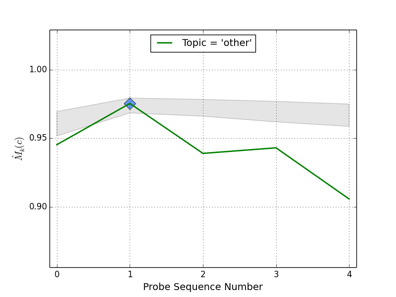
(a)

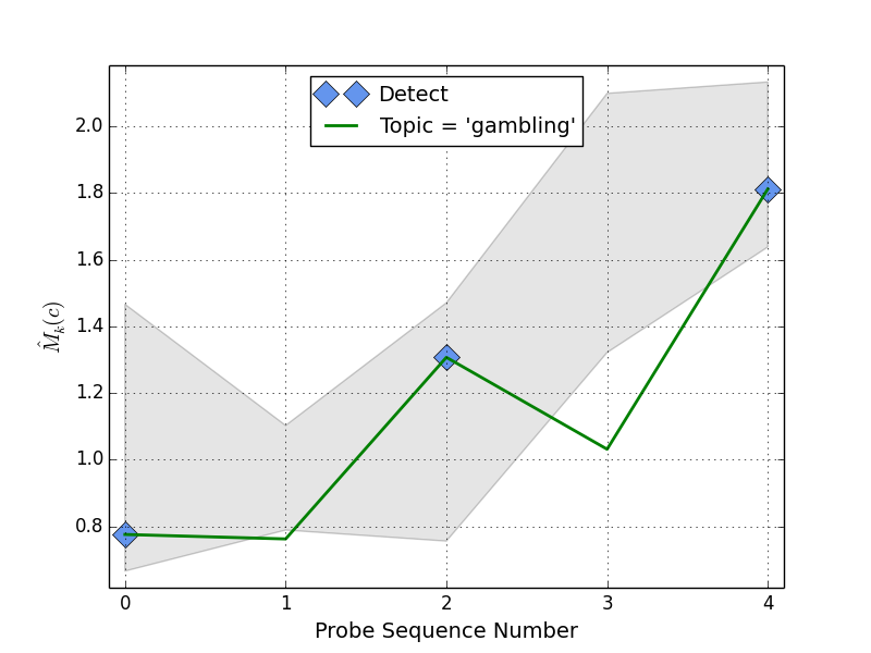
(b)

Figure 1: Illustrating detection of learning for a user session on topic gambling. Shaded areas indicate the confidence interval for $\hat{M}_{k}$ for the other topic in the upper figure, and for the gambling topic in the lower figure. Google search engine.

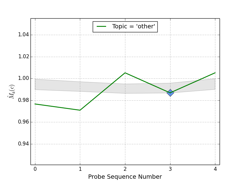
(a)

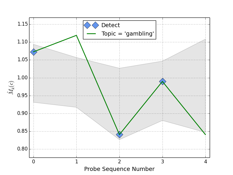
(b)

Figure 2: Illustrating detection of learning for a user session on topic gambling. Shaded areas indicate the confidence interval for $\hat{M}_{k}$ for the other topic in the upper figure, and for the gambling topic in the lower figure. Bing search engine.

The plots in Figure 1 illustrates this procedure for a user session on the topic gambling with the Google search engine. It can be seen from Figure 1(a) that $\hat{M}_{k}$ for the other topic (i.e. $\bar{c}$) quickly leaves its confidence interval as the session progresses (probe $1$ is detected as other, however the other probe queries $\{0,2,3,4\}$ lie outside the other confidence interval). In comparison, it can be seen from Figure 1(b) that $\hat{M}_{k}$ for the gambling topic (i.e. the topic which matches the user session) stays close to the confidence interval throughout the user session. The corresponding results for the Bing search engine are shown in Figure 2 and exhibit similar behaviour.

Table 6.1 summarises the detection performance on a full set of Bing and Google test data. We declare a positive detection when at least one probe query in a session of $5$ probes is detected as sensitive. For user sessions on sensitive topics it can be seen that the detection accuracy is high. For Google, $100\%$ of user sessions on a sensitive topic reject the hypothesis that no learning of the sensitive topic by the search engine has taken place and so are identified as sensitive. For Bing the corresponding detection rate is $91\%$. Recall that this hypothesis testing is being carried out based purely on the adverts in the response pages to user queries, and the queries themselves are not being used. We manually inspected a sample of the user sessions, confirming the results of Table 5.6, that the displayed adverts consistently change signficantly over the course of user sessions on sensitive topics. It is therefore reasonable to conclude that learning by the search engine has indeed occurred. That is, the rejection of the hypothesis that no learning has occured that is reported in Table 6.1 appears to be justified.

Measured detection rate of search engine learning of at least one occurence of one or more sensitive topics during a 5 probe session.

		Predicted
		Bing		Google
		Sens.	Non-sens.	Sens.	Non-sens.
Expected	Sensitive	91%	9%	100%	0%
	Non-sensitive	1%	99%	1%	99%

Table 6.1 also shows the percentage of user sessions which are sensitive but which are flagged as non-sensitive, which can be interpreted as the false negative rate. For Google, no sensitive sessions are classed as non-sensitive, and for Bing 9% are classes as non-sensitive. Also shown in the table is the percentage of user sessions which are non-sensitive but are flagged as sensitive, which can be interpreted as the false positive rate. This is low at 1% for both search engines. A manual inspection of the data shows that the first probe in a session can be misdetected sometimes, demonstrating a topic lag effect after there is a change in topic. The influence of the first probe makes it difficult to distinguish sensitive/non-sensitive based on observation of a single step. We will discuss misdetection in detail in Section 6.5.

Overall, the results in Table 6.1 indicate that the proposed approach can correctly identify potential privacy concerns for sensitive topics while keeping noise levels from false positive detections low.

We comment briefly on the difference in Table 6.1 in the measured False Negative rates for the two search engines. This difference is at least partially explained by two factors. The first is that Bing seems to be slower at adapting to changes in session topic than Google, see Section 6.5. This apparent difference in adaptation rate is also observable by comparing Figures 1(b) and 2(b), noting the differences in behaviour of the confidence intervals for the gambling topic. The second factor is differences between the search engines in the range and diversity of the available adverts across the various topics. For example, analysis of our test data shows that Google has on average $3.3$ unique adverts per probe across all topics whereas Bing has a lower average of $1.7$ unique adverts per probe. This suggests that Google’s dominant position in the search market means it may have a larger advert pool allowing more finely tuned fitting of adverts to detected topics of interest.

6.2 Individual Sensitive Topic Detection

We now evaluate the detection performance for individual sensitive topics. For each sensitive topic $c$ studied, when (i) the estimated $\hat{M}_{k}(c)$ lies inside the confidence interval for that topic and (ii) $\hat{M}_{k}(\bar{c})$ lies outside the confidence interval for the catch-all other topic (i.e. $\bar{c}$), then we say that we cannot reject the hypothesis that learning of topic $c$ has occurred.

Table 3: Measured detection rate of search engine learning of individual sensitive topics.

	Reference Topic
	anorexia	bankrupt	diabetes	disabled	divorce	gambling	gay	location	payday	prostate	unemployed
True Detect	100%	98%	100%	99%	99%	99%	98%	99%	99%	99%	99%
True Other	100%	91%	93%	93%	98%	95%	100%	87%	92%	96%	97%
False Detect	0%	9%	7%	7%	2%	5%	0%	13%	8%	4%	3%
False Other	0%	2%	0%	1%	1%	1%	2%	1%	1%	1%	1%

(a)

	Reference Topic
	anorexia	bankrupt	diabetes	disabled	divorce	gambling	gay	location	payday	prostate	unemployed
True Detect	100%	100%	96%	100%	100%	100%	100%	99%	99%	99%	100%
True Other	96%	96%	92%	100%	100%	100%	100%	100%	100%	100%	100%
False Detect	4%	4%	8%	0%	0%	0%	0%	0%	0%	0%	0%
False Other	0%	0%	4%	0%	0%	0%	0%	1%	1%	1%	0%

(b)

Table 3 summarises the detection performance for the Bing and Google test data for each of the sensitive topics studied. When evidence of learning of sensitive topic $c$ is detected and the user session is on topic $c$ then we label this a “True Detect”, otherwise we label this a “False Detect”. Conversely, when no evidence is found of topic $c$ then when the user session is in fact on topic $c$ we label this a “False Other”, otherwise we label this a “True Other”. Again, recall that the hypothesis testing here is being carried out based purely on the adverts in the response pages to probe queries.

In the Google results in Table 3(b), it can be seen that “True Detect” and “True Other” results range from $96-100\%$ across all sensitive topics. “False Detect” results, corresponding to false positives, lie in a range of $0-8\%$. “False Other” results, corresponding to false negatives, are in the range $0-4\%$. We note that topics such as bankrupt and payday tended to share adverts related to financial services, see next section, making these topics harder to distinguish from one another. This data therefore provides strong support for the assertion that detection of individual sensitive topics is indeed feasible with Google.

Table 3(a) presents the corresponding results for Bing. The “False Detect” results, corresponding to false positives, tend to be higher than for the Google data. We note that the responses for some sensitive topics overlap in terms of advert content and are not readily differentiated in our data for Bing search (as already noted, in our data set we find that Bing displays fewer unique adverts than Google). Since our test classifies all non-sensitive topics as other then sensitive topics that share adverts with other may increase the number of false positives. Overall, the detection rate for individual sensitive topics is notably high (exceeding 98%) and the false positive rate remains below 10% except for the location topic.

We next test whether probe queries can themselves generate significant levels of false positive sensitive topic detections. We constructed a test script consisting of randomly selected queries from Google Trends into which we injected the previously selected probe queries. This randomised script was executed for both Bing and Google and for each of our user configurations. Relevant result items appearing on non-probe queries were clicked. In total $1,264$ probe queries were tested for both Bing and Google using the PRI framework. Tests yielded a $0\%$ sensitive topic detection rate for any sensitive topic in combinations of search engine and users. We conclude that the selected probe queries do not themselves generate a significant amount of false sensitive topic detection.

6.3 Topic Similarity and Topic Confusion

Intuitively, we expect that some sensitive topics are similar in the sense that similar adverts tend to be associated with each. For example, the adverts prompted by the bankrupt topic, which relates to insolvency, might be expected to have some overlap with the payday topic, which relates to short-term loans.

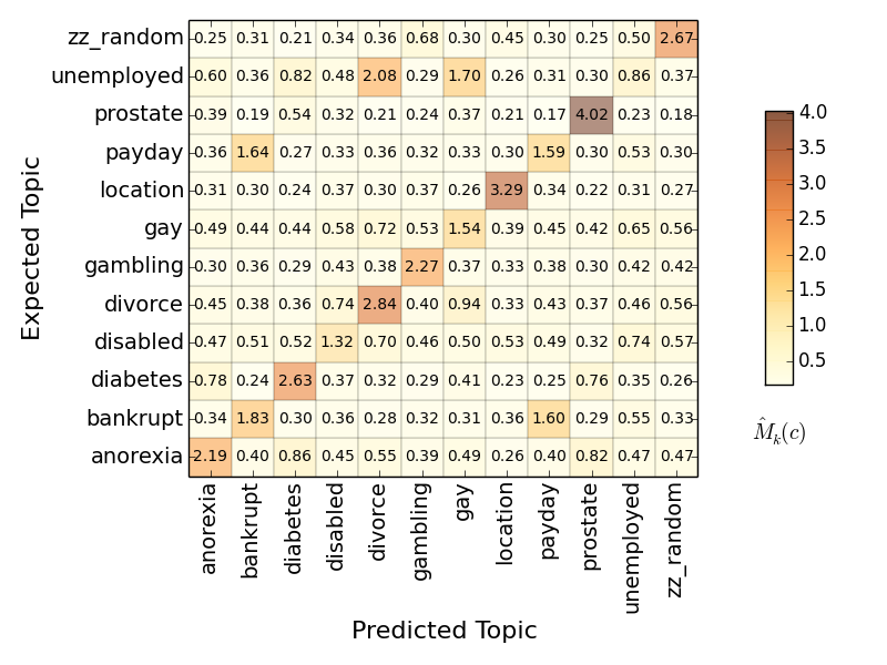
(a)

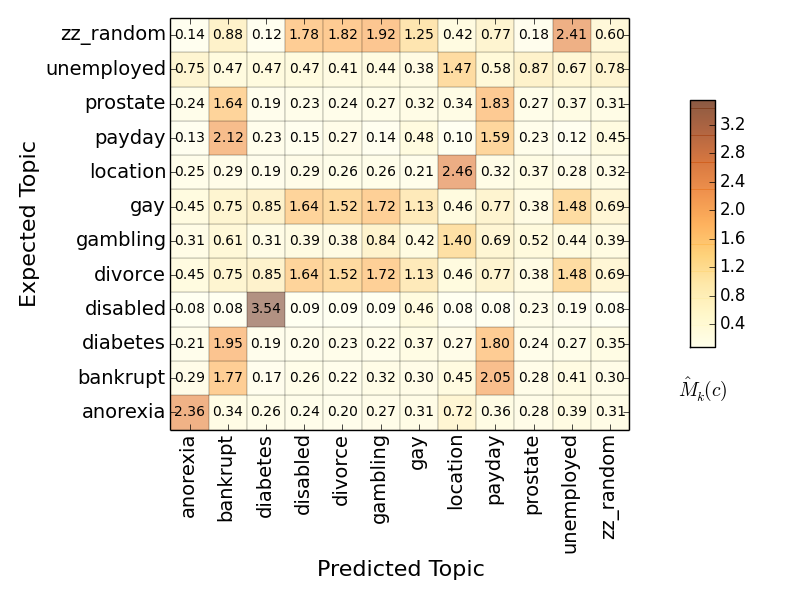
(b)

Figure 3: Average $\hat{M}_{k}(c)$ measured by topic.

We can gain some insight into this via the $\hat{M}_{k}(c)$ estimates for each topic. Figure 3 shows the average $\hat{M}_{k}(c)$ measured for each topic $c$ vs the user session topic. That is, cell $(i,j)$ shows the average $\hat{M}_{k}(c)$ measured value attained by topic $j$ when running query scripts for reference topic $i$. Each cell is heat-mapped within its row, from brightest for maximum value to darkest for lowest value per row, to improve readability. Figure LABEL:sub@fig:google_topic_matrix shows results for the Google data and Figure LABEL:sub@fig:bing_topic_matrix for the Bing data.

For the Google data, it can be seen that the maximum element in each row and column is the diagonal element, as expected from the results presented in the previous section. However, it can also be seen that the payday topic has a significantly higher $\hat{M}_{k}(c)$ value than other topics for user sessions on the bankrupt topic. Similarly, the bankrupt topic has a significantly higher $\hat{M}_{k}(c)$ value for user sessions on the payday topic. Less pronounced, but still evident, is that all health related topics tend have a higher $\hat{M}_{k}(c)$ value whenever the user session is on a health topic. For example, diabetes and prostate have elevated $\hat{M}_{k}(c)$ values for user sessions on anorexia.

For the Bing data in Figure LABEL:sub@fig:bing_topic_matrix it can be seen that the results are more complicated. As with Google, the adverts for the payday and bankrupt topics show correlated behaviour. Similarly, the adverts for health-related topics tend to be correlated. However, the Bing adverts for the disabled, divorce, gambling, gay and unemployed topics also exhibit significant correlation. This is consistent with the results in the previous section where it was observed that topics for Bing appear less readily distinguishable, possibly due to the smaller size of the pool of available adverts.

While the existence of correlation among topics is itself unsurprising, the fact that the proposed approach for detecting search engine learning is able to uncover this correlation provides additional support for the effectiveness of the approach. It also suggests that the potential exists to use the approach to infer additional information from displayed adverts. We explore this further in the following sections.

6.4 You click – therefore – I learn!

In addition to entering queries, users provide feedback to the search engine via the links that they click. Since clicking is an active step, we might expect it to influence search engine learning. Separate sets of non-click data were collected by running a single iteration of all of the test scripts on both search engines with user clicking turned off. Table 6.4 shows the percentage change in the average $\hat{M}_{k}(c)$ score for each test topic with and without user clicking of relevant search results. It can be seen that all topics had higher $\hat{M}_{k}(c)$ values when the user clicks on relevant links, suggesting that user clicks are actively used by the search engine for learning.

Percentage increase in $\hat{M}_{k}(c)$ by topic for click versus non-click. Google search data. Topic – % Increase in $\hat{M}_{k}(c)$ anorexia 49% divorce 153% payday 62% bankrupt 30% gambling 108% prostate 451% diabetes 417% gay 158% unemployed 62% disabled 57% location 63% other 233%

6.5 Time to Learn?

Inspection of the test data reveals that correct topic identification sometimes lags by one to two probes at the start of a new user session. This accounts for approximately $70\%$ of cases where “False Detects” and “False Other” results are encounted in testing. Examination of these cases provides insight into the observed speed of recommender learning, and the potential consequences for noise based privacy defences. Letting $X$ denote the random variable counting the number of consecutive misclassifications occurring together, then dividing by the total number of misclassifications we can estimate the probability that $X=1$, $X=2$, etc. This data is shown in the first column of Table 6.5. It can be seen that there are no runs of more than two misclassifications and the average length of a run of misclassifications is,

$$\mathbb{E}[X;\text{ Bing }] =1.77$$

$$\mathbb{E}[X;\text{ Google }] =1.05$$

Letting $Y$ be a random variable indicating the probe sequence number where a “False Detects” or “False Other” event first occurs, Table 6.5 reports the estinated probability that $Y=1$, $Y=2$, etc. As expected the overwhelming majority for “False Detects” and “False Other” events happen on the first probe in a session, with $\mathbb{P}(Y=1)>0.90$ for both Bing and Google.

The data in Table 6.5 therefore suggests that Google search takes an average of $1.05$ probe queries and Bing takes an average of $1.77$ probe queries to re-callibrate learning after a topic change. On average probe queries in the test data were issued after $4$ user queries. Hence, Google appears to adapt to a new topic in approximately $4$ queries, while Bing requires approximately $7$ queries. Rapid recalibration can also be seen in Table 6.5 by looking at sensitive topic classification recall for Google when successive probe queries are excluded from the calculation. When every probe query is included true positive recall is $62\%$. True positive accuracy improves once the first probe query is excluded and stabilises at $66\%$ thereafter. The false positive rates are low in all cases, falling to $0\%$ when the first three probes are excluded.

Estimated probabilities of misclassification of various lengths and probe number of first misclassification in a session. Number of Consecutive Misclassifications (X) Probe ID of First Misclassification (Y) Bing Google Bing Google $\mathbb{P}(X=1)$ 0.23 0.95 $\mathbb{P}(Y=1)$ 0.92 0.98 $\mathbb{P}(X=2)$ 0.77 0.05 $\mathbb{P}(Y=2)$ 0.03 0.01 $\mathbb{P}(X=3)$ 0.00 0.00 $\mathbb{P}(Y=3)$ 0.04 0.01 $\mathbb{P}(X=4)$ 0.00 0.00 $\mathbb{P}(Y=4)$ 0.00 0.00 $\mathbb{P}(X=5)$ 0.00 0.00 $\mathbb{P}(Y=5)$ 0.00 0.00

Recall rate by probe query excluding successive probe queries – Google. Include All Exclude $k=1$ Exclude $k=1,2$ Exclude $k=1,2,3$ True Positive 62% 66% 66% 66% False Positive 1% 1% 1% 0%

This means that a privacy defence based on random topic changes achieved, for example, by injecting spurious queries, could prove to be ineffective unless the spurious queries are repeated at intervals of less than every $4$ real queries for Google and $7$ for Bing. This is a considerable overhead.

6.6 Logged-in vs Anonymous

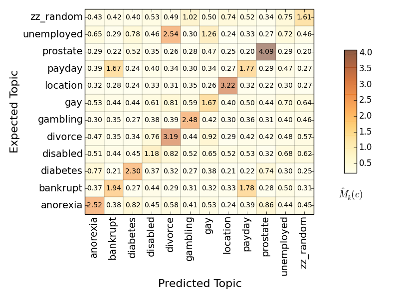
Figure 4: Average $\hat{M}_{k}(c)$ by topic. Anonymous user, Google test data

We collected data for user sessions both when the user is logged-in and when the user is anonymous. As already noted, we clean local caches and user session data between each user session.

Measured detection rate of search engine learning for an anonymous user. Predicted Bing Google Sensitive Non-sensitive Sensitive Non-sensitive Expected Sensitive 83% 0% 100% 0% Non-sensitive 17% 100% 0% 100%

Figure 4 shows the average $\hat{M}_{k}(c)$ measured for each topic for the Google search engine when the user is not logged in. It can be seen that this shows a similar overall pattern to Figure 3(a), suggesting the search engine is successful at identifying sensitive topics even in the case of an anonymous user.

Table 4: Measured detection rate of search engine learning of individual sensitive topics for an anonymous user.

	Reference Topic
	anorexia	bankrupt	diabetes	disabled	divorce	gambling	gay	location	payday	prostate	unemployed
True Detect	100%	95%	100%	98%	100%	100%	96%	100%	100%	98%	100%
True Other	100%	83%	86%	86%	100%	100%	100%	75%	100%	100%	100%
False Detect	0%	17%	14%	14%	0%	0%	0%	25%	0%	0%	0%
False Other	0%	5%	0%	2%	0%	0%	4%	1%	0%	2%	0%

(a) Bing

	Reference Topic
	anorexia	bankrupt	diabetes	disabled	divorce	gambling	gay	location	payday	prostate	unemployed
True Detect	97%	100%	100%	100%	100%	100%	100%	100%	100%	100%	100%
True Other	100%	100%	92%	100%	100%	100%	100%	100%	100%	100%	100%
False Detect	4%	0%	8%	0%	0%	0%	0%	0%	0%	0%	0%
False Other	3%	0%	0%	0%	0%	0%	0%	0%	0%	0%	0%

(b) Google

Table 6.6 shows the corresponding measured rates for sensitive/non-sensitive topic detection, which can be compared to Table 6.1. Table XIV shows the detection rate for individual topics, which can be compared to Table 3. It can be seen that the detection rates are similar to the results presented previously for logged-in users. In particular the True Detection rate for individual topics is high e.g. $97-100\%$ for Google.

We conclude that anonymity seems to provide little protection within an individual query session. The results of Section 6.5 show that the users previous search history is not really required to infer the topic of a sessions, the session itself is enough.

7 Conclusions and Discussion

With $\epsilon$-indistinguishability as a practical model for detection of user privacy risk, we show that this is readily implementable with available open tools that are simple to apply and provide highly accurate results. An appealing aspect is the use of openly available resources – Bing and Google search – a feature often missing in traditional privacy research where concerns over data disclosure limit access to potentially sensitive test data sources.

The results in this paper suggest a number of interesting avenues for future research into how to construct effective counter-measures to sensitive user profiling. The observations of learning lag in Section 6.5, the observation of low, but non-zero false positives in experimental results in Section 6, and the effect of clicking on learning in Section 6.4 appear promising for future research into effective counter-measures.

Our current experiments focus on browser-based interaction from a personal computer. In the interests of simplicity, we excluded platforms, such as mobile devices, from our current investigation. Mobile devices represent an interesting area for further investigation. The physical size of the screen on mobile and tablet devices increases the urgency to target adverts, while access to finer-grained location and usage data provides even more opportunity to target recommendations.

The user-browser interaction model chosen for this paper in Section 5.2 is based on clicking on links and subsequently navigating back to the original search page by pressing the “back” button. The user-browser interaction model can be extended in interesting ways: by allowing the user to spawn new browser tabs and new windows for example. We also removed cookies stored by the search engine during sessions to ensure observations were related to individual sessions. Allowing cookies to persist across sessions, and so potentially preserve learning effects across sessions, is another interesting variation of user-browser interaction that merits investigation.

In Section 5.2 the method for selecting probe queries in this paper based on high-occurrence terms is discussed. The resulting choice of probe queries in Section 5.2 is dependent on the choice of topics. A different choice of topics may necessitate a different choice of probe query. The approach taken in Section 5.2 is to select keywords with the highest term frequency across result pages. It is possible that other combinations of keywords may generate more informative probes, allowing more sensitive detection of search engine adaptation. How to select the most effective and informative probe queries, aligned with an individual user’s choice of topics, in a way that is not overly onerous for a user is a subject for future research.

In this paper, training set data was derived by selecting subsets of test data and deriving a dictionary of terms $D$. In a practical implementation, a predefined dictionary containing words appearing in adverts can be substituted for $D$. Frequency data for terms can then be learned either in batch mode from a pre-labelled set of example adverts, or in online mode by user labelling with new terms being added to the dictionary of terms as they are encountered. In a practical implementation some degree of online learning is desirable as adverts change over time. For example, comparison of data gathered over six month intervals indicates that as much as $30\%$ of terms used in adverts may change over that period of time.

In this paper, our goal is to inform the user by detecting evidence of privacy disclosure. In this way we hope to raise individual awareness of privacy concerns from online personalisation. A natural next step for future research is to ask what actions an individual can take to assert control in the face of privacy concerns? The varying and contextual nature of individual privacy concerns, explored in [boyd (2011)], [Panjwani et al. (2013)] and [Agarwal et al. (2013)], suggests that this is a challenge for future research.

We view this paper as a starting point towards practical user privacy in the face of ever-evolving and more powerful online systems. Future avenues of research include: looking beyond search engines to other recommender systems where content types other than adverts may provide better content for adaptation detection in the case of other recommender systems; extending $\epsilon$-indistinguishability to incorporate more complex user interaction models; constructing effective user privacy defences by exploiting observations of topic similarity and confusion encountered in our experiments, and, investigating how PRI performs for different models of contextual advert selection such as semantic or sense-based techniques that employ non-keyword based selection techniques to select adverts. In conclusion, our results indicate that evidence of adaptation is easy to find. Indeed it is mandated to maximise shareholder value. This suggests that there is an “Elephant in the Room” for privacy in the face of sophisticated of modern commercial internet systems. Namely, focusing on personal de-identification is to risk missing the larger threat of distinguishability. Our observation that such sensitive topic profiling persists even for anonymous users helps to further underline the nature of the privacy threat.

References

- [1]
- Agarwal et al. (2013) Lalit Agarwal, Nisheeth Shrivastava, Sharad Jaiswal, and Saurabh Panjwani. 2013. Do Not Embarrass: Re-examining User Concerns for Online Tracking and Advertising. In Proceedings of the Ninth Symposium on Usable Privacy and Security (SOUPS ’13). ACM, New York, NY, USA, Article 8, 13 pages. DOI:http://dx.doi.org/10.1145/2501604.2501612
- Aggarwal et al. (2010) Gaurav Aggarwal, Elie Bursztein, Collin Jackson, and Dan Boneh. 2010. An Analysis of Private Browsing Modes in Modern Browsers. In Proceedings of the 19th USENIX Conference on Security (USENIX Security’10). USENIX Association, Berkeley, CA, USA, 6–6. http://dl.acm.org/citation.cfm?id=1929820.1929828
- Backes et al. (2012) Michael Backes, Aniket Kate, Matteo Maffei, and Kim Pecina. 2012. ObliviAd: Provably Secure and Practical Online Behavioral Advertising. In Proceedings of the 2012 IEEE Symposium on Security and Privacy (SP ’12). IEEE Computer Society, Washington, DC, USA, 257–271. DOI:http://dx.doi.org/10.1109/SP.2012.25
- Bird et al. (2009) Steven Bird, Ewan Klein, and Edward Loper. 2009. Natural Language Processing with Python (1st ed.). O’Reilly Media, Inc.
- boyd (2011) danah boyd. June 6,2011. Networked Privacy. (June 6,2011).
- Commission (2015) U.S. Equal Employment Opportunity Commission. 2015. Types of Discrimination. (2015). (Retrieved on March 21, 2015 from http://www.eeoc.gov/laws/types/).
- Datta (2014) Anupam Datta. 2014. Privacy Through Accountability: A Computer Science Perspective. In Proceedings of the 10th International Conference on Distributed Computing and Internet Technology - Volume 8337 (ICDCIT 2014). Springer-Verlag New York, Inc., New York, NY, USA, 43–49. DOI:http://dx.doi.org/10.1007/978-3-319-04483-5_5
- Erkin et al. (2010) Zekeriya Erkin, Michael Beye, Thijs Veugen, and Reginald L. Lagendijk. 2010. Privacy enhanced recommender system. In 31st Symposium on Information Theory in the Benelux, WIC 2010. IEEE Benelux Information Theory Chapter, 35–42. http://doc.utwente.nl/87258/
- Erkin et al. (2011) Zekeriya Erkin, Michael Beye, Thijs Veugen, and Reginald L Lagendijk. 2011. Efficiently computing private recommendations. In Acoustics, Speech and Signal Processing (ICASSP), 2011 IEEE International Conference on. IEEE, 5864–5867.
- Foundation (2015a) Electronic Frontier Foundation. Retrieved: 25-09-2015a. https://www.eff.org/privacybadger. (Retrieved: 25-09-2015).
- Foundation (2015b) Electronic Frontier Foundation. Retrieved: 25-09-2015b. https://www.google.com/intl/en/policies/privacy/?fg=1. (Retrieved: 25-09-2015).
- Foundation (2015c) Mozilla Foundation. Retrieved: 25-09-2015c. https://www.mozilla.org/en-US/lightbeam/. (Retrieved: 25-09-2015).
- Google (2015) Google. 2015. Google Trends. Retrieved on March 21, 2015 from http://www.google.com/trends/. (2015).
- Graph (2015) Google Knowledge Graph. Retrieved: 30-09-2015. http://googleblog.blogspot.co.uk/2012/05/introducing-knowledge-graph-things-not.html. (Retrieved: 30-09-2015).
- Guha et al. (2010) Saikat Guha, Bin Cheng, and Paul Francis. 2010. Challenges in Measuring Online Advertising Systems. In Proceedings of the 10th ACM SIGCOMM Conference on Internet Measurement (IMC ’10). ACM, New York, NY, USA, 81–87. DOI:http://dx.doi.org/10.1145/1879141.1879152
- Guha et al. (2011) Saikat Guha, Bin Cheng, and Paul Francis. 2011. Privad: Practical Privacy in Online Advertising. In Proceedings of the 8th USENIX Conference on Networked Systems Design and Implementation (NSDI’11). USENIX Association, Berkeley, CA, USA, 169–182. http://dl.acm.org/citation.cfm?id=1972457.1972475
- Hannak et al. (2013) Aniko Hannak, Piotr Sapiezynski, Arash Molavi Kakhki, Balachander Krishnamurthy, David Lazer, Alan Mislove, and Christo Wilson. 2013. Measuring Personalization of Web Search. In Proceedings of the 22Nd International Conference on World Wide Web (WWW ’13). International World Wide Web Conferences Steering Committee, Republic and Canton of Geneva, Switzerland, 527–538. http://dl.acm.org/citation.cfm?id=2488388.2488435
- Howe et al. (2009) Daniel C Howe, Helen Nissenbaum, and Vincent Toubiana. 2009. TrackMeNot. mrl. nyu. edu/dhower/trackmenot (2009).
- Idris (2012) Ivan Idris. 2012. NumPy Cookbook. Packt Publishing.
- iSense (2015) iSense. Retrieved: 30-09-2015. http://www.isense.net. (Retrieved: 30-09-2015).
- Jansen et al. (2013) Bernard J Jansen, Zhe Liu, and Zach Simon. 2013. The effect of ad rank on the performance of keyword advertising campaigns. Journal of the American Society for Information Science and Technology 64, 10 (2013), 2115–2132.
- Langville and Meyer (2006) Amy N. Langville and Carl D. Meyer. 2006. Google’s PageRank and Beyond: The Science of Search Engine Rankings. Princeton University Press, Princeton, NJ, USA.
- Lécuyer et al. (2014) Mathias Lécuyer, Guillaume Ducoffe, Francis Lan, Andrei Papancea, Theofilos Petsios, Riley Spahn, Augustin Chaintreau, and Roxana Geambasu. 2014. XRay: Enhancing the Web’s Transparency with Differential Correlation. In Proceedings of the 23rd USENIX Conference on Security Symposium (SEC’14). USENIX Association, Berkeley, CA, USA, 49–64. http://dl.acm.org/citation.cfm?id=2671225.2671229
- Lempel and Moran (2005) Ronny Lempel and Shlomo Moran. 2005. Rank-stability and rank-similarity of link-based web ranking algorithms in authority-connected graphs. Information Retrieval 8, 2 (2005), 245–264.
- Ohm (2010) Paul Ohm. 2010. Broken promises of privacy: Responding to the surprising failure of anonymization. UCLA Law Review 57 (2010), 1701.
- Panjwani et al. (2013) Saurabh Panjwani, Nisheeth Shrivastava, Saurabh Shukla, and Sharad Jaiswal. 2013. Understanding the Privacy-personalization Dilemma for Web Search: A User Perspective. In Proceedings of the SIGCHI Conference on Human Factors in Computing Systems (CHI ’13). ACM, New York, NY, USA, 3427–3430. DOI:http://dx.doi.org/10.1145/2470654.2466470
- Pariser (2011) Eli Pariser. 2011. The Filter Bubble: What the Internet Is Hiding from You. Penguin Group , The.
- Peddinti and Saxena (2011) Sai Teja Peddinti and Nitesh Saxena. 2011. On the limitations of query obfuscation techniques for location privacy. In Proceedings of the 13th international conference on Ubiquitous computing. ACM, 187–196.
- Pedregosa et al. (2011) F. Pedregosa, G. Varoquaux, A. Gramfort, V. Michel, B. Thirion, O. Grisel, M. Blondel, P. Prettenhofer, R. Weiss, V. Dubourg, J. Vanderplas, A. Passos, D. Cournapeau, M. Brucher, M. Perrot, and E. Duchesnay. 2011. Scikit-learn: Machine Learning in Python. Journal of Machine Learning Research 12 (2011), 2825–2830.
- Ramakrishnan et al. (2001) Naren Ramakrishnan, Benjamin J Keller, Batul J Mirza, Ananth Y Grama, and George Karypis. 2001. Privacy Risks in Recommender Systems. IEEE Internet Computing 5, 6 (2001), 54–62.
- Ricci et al. (2010) Francesco Ricci, Lior Rokach, Bracha Shapira, and Paul B. Kantor. 2010. Recommender Systems Handbook (1st ed.). Springer-Verlag New York, Inc., New York, NY, USA.
- Richardson et al. (2007) Matthew Richardson, Ewa Dominowska, and Robert Ragno. 2007. Predicting clicks: estimating the click-through rate for new ads. In Proceedings of the 16th international conference on World Wide Web. ACM, 521–530.
- Schwartz and Solove (2011) Paul M Schwartz and Daniel J Solove. 2011. PII Problem: Privacy and a New Concept of Personally Identifiable Information, The. NYUL Rev. 86 (2011), 1814.
- Spiliopoulou et al. (2012) Myra Spiliopoulou, Bamshad Mobasher, Olfa Nasraoui, and Osmar Zaiane. 2012. Guest editorial: special issue on a decade of mining the Web. Data Mining and Knowledge Discovery 24, 3 (2012), 473–477. DOI:http://dx.doi.org/10.1007/s10618-012-0257-y
- Sweeney (2013) Latanya Sweeney. 2013. Discrimination in Online Ad Delivery. Queue 11, 3, Article 10 (March 2013), 20 pages. DOI:http://dx.doi.org/10.1145/2460276.2460278
- Zemanta (2015) Zemanta. Retrieved: 30-09-2015. http://www.zemanta.com. (Retrieved: 30-09-2015).