Trust, but Verify: Two-Phase Typing for Dynamic Languages

Abstract.

A key challenge when statically typing so-called dynamic languages is the ubiquity of value-based overloading, where a given function can dynamically reflect upon and behave according to the types of its arguments. Thus, to establish basic types, the analysis must reason precisely about values, but in the presence of higher-order functions and polymorphism, this reasoning itself can require basic types. In this paper we address this chicken-and-egg problem by introducing the framework of two-phased typing. The first “trust” phase performs classical, i.e. flow-, path- and value-insensitive type checking to assign basic types to various program expressions. When the check inevitably runs into “errors” due to value-insensitivity, it wraps problematic expressions with DEAD-casts, which explicate the trust obligations that must be discharged by the second phase. The second phase uses refinement typing, a flow- and path-sensitive analysis, that decorates the first phase’s types with logical predicates to track value relationships and thereby verify the casts and establish other correctness properties for dynamically typed languages.

1. Introduction

Higher-order constructs are increasingly adopted in dynamic scripting languages, as they facilitate the production of clean, correct and maintainable code. Consider, for example, the following (first-order) JavaScript function

⬇

function minIndexFO(a) {

if (a.length $\leq$ 0)

return -1;

var min = 0;

for (var i = 0; i < a.length; i++) {

if (a[i] < a[min])

min = i;

}

return min;

}

which computes the index of the minimum value in the array a by looping over the array, updating the min value with each index i whose value a[i] is smaller than the “current” a[min]. Modern dynamic languages let programmers factor the looping pattern into a higher-order $reduce function (Figure 1), which frees them from manipulating indices and thereby prevents the attendant “off-by-one” mistakes. Instead, the programmer can compute the minimum index by supplying an appropriate f to reduce as in minIndex shown at the right of Figure 1.

⬇

function $reduce(a, f, x) {

var res = x, i = 0;

for (i = 0; i < a.length; i++)

res = f(res, a[i], i++);

return res;

}

function reduce(a, f, x) {

if (arguments.length === 3)

return $reduce(a, f, x);

return $reduce(a, f, a[0]);

}

⬇

function minIndex(a) {

if (a.length $\leq$ 0)

return -1;

function step(min, cur, i) {

return cur < a[min] ? i:min;

}

return reduce(a, step, 0);

}

Figure 1. Computing the minimum-valued index with Higher-Order Functions

This trend towards abstraction and reuse poses a challenge to static program analyses: how to precisely trace value relationships across higher-order functions and containers? A variety of dataflow- or abstract interpretation- based analyses could be used to verify the safety of array accesses in minIndexFO by inferring the loop invariant that i and min are between 0 and a.length. Alas, these analyses would fail on minIndex. The usual methods of procedure summarization apply to first-order functions, and it is not clear how to extend higher-order analyses like CFA to track the relationships between the values and closures that flow to $reduce.

An Approach: Refinement Types.

Refinement types [31] hold the promise of a precise and compositional analysis for higher-order functions. Here, basic types are decorated with refinement predicates that constrain the values inhabiting the type. For example, we can define

⬇

type idx<x> = {v:number | 0 $\leq$ v && v < len(x) }

to denote the set of valid indices for an array x and can be used to type $reduce as

⬇

$reduce :: <A,B>(a: A[], f: (B,A,idx<a>) $\Rightarrow$ B, x: B) $\Rightarrow$ B

The above type is a precise relational summary of the behavior of $reduce: the higher-order f is only invoked with valid indices for a. Consequently, step is only called with valid indices for a, which ensures array safety.

Problem: Value-based Overloading.

A main attraction of dynamic languages is value-based overloading, where syntactic entities (e.g. variables) may be bound to multiple types at run-time, and furthermore, computations may be customized to particular types, by reflecting on the values bound to variables. For example, it is common to simplify APIs by overloading the reduce function to make the initial value x optional; when omitted, the first array element a[0] is used instead. Here, reduce really has two different function types: one with 3 parameters and another one with 2. Furthermore, reduce reflects on the size of arguments to select the behavior appropriate to the calling context.

Value-based overloading conflicts with a crucial prerequisite for refinements, namely that the language possesses an unrefined static type system that provides basic invariants about values which can then be refined using logical predicates. Unfortunately, as shown by reduce, to soundly establish basic typing we must reason about the logical relationships between values, which, ironically, is exactly the problem we wished to solve via refinement typing. In other words, value-based overloading creates a chicken-and-egg problem: refinements require us to first establish basic typing, but the latter itself requires reasoning about values (and hence, refinements!).

Solution: Trust but Verify.

We introduce two-phased typing, a new strategy for statically analyzing dynamic languages. The key insight is that we can completely decouple reasoning about basic types and refinements into distinct phases by converting “type errors” from the first phase into “assertion failures” for the second. Two-phase typing starts with a source language where value-based overloading is specified using intersections and (untagged) unions of the different possible (run-time) types.

The first phase performs classical, i.e. flow-, path- and value-insensitive type checking to assign basic types to various program expressions. When the check inevitably runs into “errors” due to value-insensitivity, it wraps problematic expressions with DEAD-casts which allow the first phase to proceed, trusting that the expressions have the casted types. In other words, the first phase elaborates [10] the source language with intersection and (untagged) union types, into a target ML-like language with classical products, (tagged) sums and DEAD-casts, which explicate the trust obligations that must be discharged by the second phase. The second phase carries out refinement, i.e. flow- and path-sensitive inference, to decorate the basic types (from the first phase) with predicates that precisely track relationships about values, and uses the refinements to verify the casts and other properties, discharging the assumptions of the first phase.

For example, reduce is described as the intersection of two contexts, i.e. function types which take two and three parameters respectively. The trust-phase checks the body under both contexts (separately). In each context, one of the calls to $reduce is “ill-typed”. In the context where the function takes two inputs, the call using x is undefined; when the function takes three inputs, there is a mismatch in the types of f and a[0]. Consequently, each ill-typed expression is wrapped with a cast which obliges the verify phase to prove that the call is dead code in that context, thereby verifying overloading in a cooperative manner.

Benefits.

While it is possible to account for value-based overloading in a single phase, the currently known methods that do so are limited to the extremes of types and program logics. At one end, systems like Typed Racket [28] and Flow Typing [16] extend classical type systems to account for a fixed set of typeof-style tests, but cannot reason about general value tests (e.g. the size of arguments) that often appear in idiomatic code. At the other end, systems like System D [7] embed the typing relation in an expressive program logic, allowing general value tests, but give up on basic type structure, thereby sacrificing inference, causing a significant annotation overhead. In contrast, our approach separates the concerns of basic typing and reasoning about values, thereby yielding several concrete benefits by modularizing specification, verification and soundness.

• Specification: Instead of a fixed set of type-tests, two-phase typing handles complex value relationships which can be captured inside refinements in an expressive logic. Furthermore, the expressiveness of the basic type system and logics can be extended independently, e.g. to account for polymorphism, classes or new logical theories, directly yielding a more expressive specification mechanism.

• Verification: Two-phase typing enables the straightforward composition of simple type checkers (uncomplicated by reasoning about values) with program logics (relying upon the basic invariants provided by typing – e.g. the parametric polymorphism needed to verify minIndex). Furthermore, two-phase typing allows us to compose basic typing with abstract interpretation [23], which drastically lowers the annotation burden for using refinement types.

• Soundness: Finally, our elaboration-based approach makes it straightforward to establish soundness for two-phased typing. The first phase ignores values and refinements, so we can use classical methods to prove the elaborated target is “equivalent to” the source. The second phase uses standard refinement typing techniques on the well-typed elaborated target, and hence lets us directly reuse the soundness theorems for such systems [18] to obtain end-to-end soundness for two-phased typing.

Contributions.

Concretely, in this paper we make the following contributions. First, we informally illustrate (§ 2) how two-phase typing lets us statically analyze dynamic, value-based overloading patterns drawn from real-world code, where, we empirically demonstrate, value-based overloading is ubiquitous. Second, we formalize two-phase typing using a core calculus, Rsc, whose syntax and semantics are detailed in § 3. Third, we formalize the first phase (§ 4), which elaborates [10] a source language with value-based overloading into a target language with DEAD-casts in lieu of overloading. We prove that the elaborated target preserves the semantics of the source, i.e. the DEAD-casts fail iff the source would hit a type error at run time. Finally, we demonstrate how standard refinement typing machinery can be applied to the elaborated well-typed target (§ 5) to statically verify the DEAD-casts, yielding end-to-end soundness for our system.

2. Overview

We begin with an overview illustrating how we soundly verify value-based overloading using our novel two-phased approach.

2.1. Value-based Overloading

⬇

neg :: (number, number) $\Rightarrow$ number

/\ (number, boolean) $\Rightarrow$ boolean

function neg(flag, x) {

if (flag) return 0-x;

return !x;

}

⬇

var a = neg(1,1); // OK

var b = neg(0,true); // OK

var c = neg(0,1); // ERR

var d = neg(1,true); // ERR

Figure 2. An example program with value-based overloading

Consider the code in Figure 2. The function neg behaves as follows. When a number is passed as input, indicated by passing in a non-zero, i.e. “truthy” flag, the function flips its sign by subtracting the input from 0. Instead, when a boolean is passed in, indicated by a zero, i.e. “falsy” flag, the function returns the boolean negation. Hence, the calls made to assign a and b are legitimate and should be statically accepted. However, the calls made to assign c and d lead to run-time errors (assuming we eschew implicit coercions), and hence, should be rejected.

The function neg distils value-based overloading to its essence: a run-time test on one parameter’s value is used to determine the type of, and hence the operation to be applied to, another value. Of course in JavaScript, one could use a single parameter and the typeof operator for this particular simple case, and design analyses targeted towards a fixed set of type tests, e.g. using variants of the typeof operator [28, 16]. However, arbitrary value tests – such as tests of the size of arguments shown in reduce in Figure 1 – can be and are used in practice. Thus, we illustrate the generality of the problem and our solution without using the typeof operator (which is a special case of our solution).

Prevalence of Value-based Overloading.

The code from Figure 1 is not a pathological toy example. It is adapted from the widely used D3 visualization library. The advent of TypeScript makes it possible to establish the prevalence of value-based overloading in real-world libraries, as it allows developers to specify overloaded signatures for functions. (Even though TypeScript does not verify those signatures, it uses them as trusted interfaces for external JavaScript libraries and code completion.) The Definitely Typed repository  contains TypeScript interfaces for a large number of popular JavaScript libraries. We analyzed the TypeScript interfaces to determine the prevalence of value-based overloading. Intuitively, every function or method with multiple (overloaded) signatures or optional arguments has an implementation that uses value-based overloading.

Figure 3 summarizes the results of our study. On the left, we show the fraction of overloaded functions in the 10 benchmarks analyzed by Feldthaus et al. [12]. The data shows that over 25% of the functions in 4 of 10 libraries use value-based overloading, and an even larger fraction is overloaded in libraries like jquery and d3. On the right we summarize the occurrence of overloading across all the libraries in Definitely Typed. The data shows, for example, that in more than 25% of the libraries, more than 25% of the functions are overloaded with multiple types. The figure jumps to nearly 55% of functions if we also include optional arguments.

File	#Funs	%Ovl	%Opt	%Any
[filter=ace/ace.d.ts fabricjs/fabricjs.d.ts jquery/jquery.d.ts underscore/underscore.d.ts pixi/pixi.d.ts box2d/box2dweb.d.ts leaflet/leaflet.d.ts threejs/three.d.ts d3/d3.d.ts sugar/sugar.d.ts, late after line=
, late after last line=

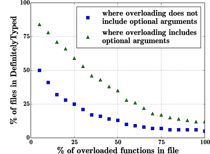
Figure 3. The prevalence of value-based overloading. (L) Libraries from [12]: #Funs is the number of functions in the signature, %Ovl is %-functions with multiple signatures, %Opt is %-functions with optional arguments, and %Any is %-functions with either of these features. (R) Overloading across all files in DefinitelyTyped. A point $(x,y)$ means $y\%$ of files have more than $x\%$ overloaded functions.

The signatures in Definitely Typed have not been soundly checked against their implementations. Hence, it is possible that they mischaracterize the semantics of the actual code, but modulo this caveat, we believe the study demonstrates that value-based overloading is ubiquitous, and so to soundly and statically analyze dynamic languages, it is crucial that we develop techniques that can precisely and flexibly account for it.

2.2. Refinement Types

Types and Refinements.

A basic refinement type $T$ is a basic type, e.g. number, refined with a logical formula from an SMT decidable logic – for the purposes of this paper, the quantifier-free logic of uninterpreted functions and linear integer arithmetic (QF_UFLIA [25]). For example, {v:number | v != 0} describes the subset of numbers that are non-zero. We write $A$ to abbreviate the trivially refined type ${\{{\nu}\!:\!{A}\mid\textit{true}\}}$, e.g. number is an abbreviation for ${\{{\nu}\!:\!{\texttt{\color[rgb]{0,0.4,0}number}}\mid\textit{true}\}}$.

Summaries: Function Types.

We can specify the behavior of functions with refined function types, of the form

$$({{x}_{1}:{T}_{1},\ldots,{x}_{n}:{T}_{n}})\Rightarrow{T}$$

where arguments are named $x_{i}$ and have types $T_{i}$ and the output is a $T$. In essence, the input types $T_{i}$ specify the function’s preconditions, and the output type $T$ describes the postcondition. Furthermore, each input type and the output type can refer to the arguments $x_{i}$ which yields precise function contracts. For example,

$$({{{x}\!:\!{0\leq x}}})\Rightarrow{{\{{\nu}\!:\!{\texttt{\color[rgb]{0,0.4,0}number}}\mid x<\nu\}}}$$

is a function type that describes functions that require a non-negative input, and ensure that the output is greater than the input.

Example.

Returning to neg in Figure 2, we can define two refinements of number:

⬇

type tt = {v:number | v != 0} // "truthy" numbers

type ff = {v:number | v = 0} // "falsy" numbers

which are used to specify a refined type for neg shown on the left in Figure 4.

Problem: A Circular Dependency.

While it is easy enough to specify a type signature, it is another matter to verify it, and yet another matter to ensure soundness. The challenge is that value-based overloading introduces a circular dependency between types and refinements. The soundness of basic types requires (i.e. is established by) the refinements, while the refinements themselves require (i.e. are attached to) basic types. In classical refinement systems like DML [31], basic types are established without requiring refinements. A classical refinement system is thus a conservative extension of the corresponding non-refined language, i.e. removing the refinements from a DML program, yields valid, well-typed ML. Unfortunately, value-based overloading removes this crucial property, posing a circular dependency between types and refinements.

Solution: Two-Phase Checking.

We break the cycle by typing programs in two phases. In the first, we trust the basic types are correct and use them (ignoring the refinements) to elaborate source programs into a target overloading-free language. Inevitably, value-based overloading leads to “errors” when typing certain sub-expressions in the wrong context, e.g. subtracting a boolean-valued x from 0. Instead of rejecting the program, the elaboration wraps ill-typed expressions with DEAD-casts, which are assertions stating the program is well-typed assuming those expressions are dead code. In the second phase we reuse classical refinement typing techniques to verify that the DEAD-casts are indeed unreachable, thereby discharging the assumptions made in the first phase.

⬇

neg :: (tt, number) $\Rightarrow$ number

/\ (ff, boolean) $\Rightarrow$ boolean

function neg(flag, x) {

if (flag) return 0-x;

return !x;

}

var a = neg(1,1); //OK

var b = neg(0,true); //OK

var c = neg(0,1); //ERR

var d = neg(1,true); //ERR

⬇

neg#1 :: (tt, number) $\Rightarrow$ number

function neg#1(flag, x) {

if (flag) return 0-x;

return !DEAD(x);

}

neg#2 :: (ff, boolean) $\Rightarrow$ boolean

function neg#2(flag, x) {

if (flag) return 0-DEAD(x);

return !x;

}

var neg = (neg#1, neg#2);

var a = fst(neg)(1,1); //OK

var b = snd(neg)(0,true); //OK

var c = fst(neg)(0,1); //ERR

var d = snd(neg)(1,true); //ERR

Figure 4. Source program (l) and target (r) resulting from first phase elaboration.

2.3. Phase 1: Trust

The first phase elaborates the source program into an equivalent typed target language with two key properties: First, the target program is simply typed – i.e. has no union or intersection types, but just classical ML-style sums and products. Second, source-level type errors are elaborated to target-level DEAD-casts. The right side of Figure 4 shows the elaboration of the source from the left side. While we formalize the elaboration declaratively using a single judgment form (§ 4), it comprises two different steps. Critically, each step, and hence the entire first phase, is independent of the refinements – they are simply carried along unchanged.

A. Clone.

In the first step, we create separate clones of each overloaded function, where each clone is assigned a single conjunct of the original overloaded type. For example, we create two clones neg#1 and neg#2 respectively typed using the two conjuncts of the original neg. The binder neg is replaced with a tuple of its clones. Finally, each use of neg extracts the appropriate element from the tuple before issuing the call.

Since the trust phase must be independent of refinements, the overload resolution in this step uses only the basic types at the call-site to determine which of the two clones to invoke. For example, in the assignment to a, the source call neg(1,1) – which passes in two number values, and hence, matches the first overload (conjunct) – is elaborated to the target call fst(neg)(1,1). In the assignment to d, the source call neg(1,true) – which passes in a number and a boolean, and hence matches the second overload – is elaborated to the target call snd(neg)(1,true), even though 1 does not have the refined type ff.

B: Cast.

In the second step we check – using classical, unrefined type checking – that each clone adheres to its specified type. Unlike under usual intersection typing [22, 10], in our context these checks almost surely “fail”. For example, neg#1 does not type-check as the parameter x has type number and so we cannot compute !x. Similarly, neg#2 fails because x has type boolean and so 0-x is erroneous. Rather than reject the program, we wrap such failures with DEAD-casts. For example, the above occurrences of x elaborate to $\texttt{DEAD}(\texttt{x})$ on the right in Figure 4.

Intuitively, the value relationships established at the call-sites and guards ensure that the failures will not happen at run-time. However, recall that the first phase’s goal is to decouple reasoning about types from reasoning about values. Hence, we just trust all the types but use DEAD-casts to explicate the value-relationship obligations that are needed to establish typing: namely that the DEAD-casts are indeed dead code.

2.4. Phase 2: Verify

The second phase takes as input the elaborated program emitted by the first phase, which is essentially a classical well-typed ML program with assertions and without any value-overloading. Hence, the second phase can use any existing program logic [14, 4], refinement typing [31, 18, 23, 2], or contracts & abstract interpretation [20] to check that the target’s assertions never fail, which, we prove, ensures that the source is type-safe.

To analyze programs with closures, collections and polymorphism, (e.g. minIndex from Figure 1) we perform the second phase using the refinement types that are carried over unchanged by the elaboration process of the first phase. Intuitively, refinement typing can be viewed as a generalization of classical program logics where assertions are generalized to type bindings, and the rule of consequence is generalized as subtyping. While refinement typing is a previously known technique, to make the paper self-contained, we illustrate how the second phase verifies the DEAD-casts in Figure 4.

Refinement Type Checking.

A refinement type checker works by building up an environment of type bindings that describe the machine state at each program point, and by checking that at each call-site, the actual argument’s type is a refined subtype of the expected type for the callee, under the context described by the environment at that site. The subtyping relation for basic types is converted to a logical verification condition whose validity is checked by an SMT solver. The subtyping relation for compound types (e.g. functions, collections) is decomposed, via co- and contra-variant subtyping rules, into subtyping constraints over basic types, which can be discharged as above.

Typing DEAD-Casts.

To use a standard refinement type checker for the second phase of verification, we only need to treat DEAD as a primitive operation with the refined type:

$$\texttt{DEAD}::\forall{A,B}.({{\{{\nu}\!:\!{A}\mid\textit{false}\}}})\Rightarrow{B}$$

That is, we assign DEAD the precondition false which states there are no valid inputs for it, i.e. that it should never be called (akin to assert(false) in other settings).

Environments.

To verify DEAD-casts, the refinement type checker builds up an environment of type binders describing variables and branch conditions that are in scope at each program point. For example, the DEAD call in neg#1, has the environment:

$$\Gamma_{1}\ \doteq \ {{\texttt{flag}}\!:\!{\texttt{\color[rgb]{0,0.4,0}tt}}},\ {{\texttt{x}}\!:\!{\texttt{\color[rgb]{0,0.4,0}number}}},\ {{\texttt{g}_{1}}\!:\!{{\{{\nu}\!:\!{\texttt{\color[rgb]{0,0.4,0}boolean}}\mid\texttt{flag}=0\}}}}$$ (1)

where the first two bindings are the function parameters, whose types are the input types. The third binding is from the “else” branch of the flag test, asserting the branch condition flag is “falsy” i.e. equals $0$. At the DEAD call in neg#2 the environment is:

$$\Gamma_{2}\ \doteq \ {{\texttt{flag}}\!:\!{\texttt{\color[rgb]{0,0.4,0}ff}}},\ {{\texttt{x}}\!:\!{\texttt{\color[rgb]{0,0.4,0}boolean}}},\ {{\texttt{g}_{1}}\!:\!{{\{{\nu}\!:\!{\texttt{\color[rgb]{0,0.4,0}boolean}}\mid\texttt{flag}\not=0\}}}}$$ (2)

At the assignments to a, b and c the environments are respectively:

$$\Gamma_{a}\ \doteq \ {{\texttt{\color[rgb]{0,0,0.75}neg}}\!:\!{T_{\texttt{\color[rgb]{0,0,0.75}neg}}}}$$ (3)

$$\Gamma_{b}\ \doteq \ \Gamma_{a},\ {{\texttt{a}}\!:\!{\texttt{\color[rgb]{0,0.4,0}number}}}$$ (4)

$$\Gamma_{c}\ \doteq \ \Gamma_{b},\ {{\texttt{b}}\!:\!{\texttt{\color[rgb]{0,0.4,0}boolean}}}$$ (5)

where $$T_{\texttt{\color[rgb]{0,0,0.75}neg}}$$ abbreviates the product type of the (elaborated) tuple neg.

$$T_{\texttt{\color[rgb]{0,0,0.75}neg}}\ \doteq \ (({\texttt{\color[rgb]{0,0.4,0}tt},\texttt{\color[rgb]{0,0.4,0}number}})\Rightarrow{\texttt{\color[rgb]{0,0.4,0}number}})\ \mathsf{\times}\ (({\texttt{\color[rgb]{0,0.4,0}ff},\texttt{\color[rgb]{0,0.4,0}boolean}})\Rightarrow{\texttt{\color[rgb]{0,0.4,0}boolean}})$$ (6)

Subtyping.

At each function call-site, the refinement type system checks that the actual argument is indeed a subtype of the expected one. For example, the DEAD calls inside neg#1 and neg#2 yield the respective subtyping obligation:

$$\Gamma_{1} \vdash\ {\{{\nu}\!:\!{\texttt{\color[rgb]{0,0.4,0}number}}\mid\nu=\texttt{x}\}} \ \sqsubseteq\ {\{{\nu}\!:\!{\texttt{\color[rgb]{0,0.4,0}number}}\mid\textit{false}\}}$$ (7)

$$\Gamma_{2} \vdash\ {\{{\nu}\!:\!{\texttt{\color[rgb]{0,0.4,0}boolean}}\mid\nu=\texttt{x}\}} \ \sqsubseteq\ {\{{\nu}\!:\!{\texttt{\color[rgb]{0,0.4,0}boolean}}\mid\textit{false}\}}$$ (8)

The obligation states that the type of the argument x should be a subtype of the input type of DEAD. Similarly, at the assignments to a, b and c the first arguments generate the respective subtyping obligations:

$$\Gamma_{a} \vdash\ {\{{\nu}\!:\!{\texttt{\color[rgb]{0,0.4,0}number}}\mid\nu=1\}} \ \sqsubseteq\ {\{{\nu}\!:\!{\texttt{\color[rgb]{0,0.4,0}number}}\mid\nu\not=0\}}$$ (9)

$$\Gamma_{b} \vdash\ {\{{\nu}\!:\!{\texttt{\color[rgb]{0,0.4,0}number}}\mid\nu=0\}} \ \sqsubseteq\ {\{{\nu}\!:\!{\texttt{\color[rgb]{0,0.4,0}number}}\mid\nu=0\}}$$ (10)

$$\Gamma_{c} \vdash\ {\{{\nu}\!:\!{\texttt{\color[rgb]{0,0.4,0}number}}\mid\nu=0\}} \ \sqsubseteq\ {\{{\nu}\!:\!{\texttt{\color[rgb]{0,0.4,0}number}}\mid\nu\not=0\}}$$ (11)

Verification Conditions.

To verify subtyping obligations, we convert them into logical verification conditions (VCs), whose validity determines whether the subtyping holds. A subtyping obligation ${\Gamma\vdash{\{{\nu}\!:\!{b}\mid p\}}\sqsubseteq{\{{\nu}\!:\!{b}\mid q\}}}$ translates to the VC ${[\![\Gamma]\!]\Rightarrow(p\Rightarrow q)}$ where $[\![\Gamma]\!]$ is the conjunction of the refinements of the binders in $\Gamma$. For example, the subtyping obligations (7) and (8) yield the respective VCs:

$$(\texttt{flag}\not=0\wedge\textit{true}\wedge\texttt{flag}=0) \Rightarrow\ {\nu=\texttt{x}} \ \Rightarrow\ {\textit{false}}$$ (12)

$$(\texttt{flag}=0\wedge\textit{true}\wedge\texttt{flag}\not=0) \Rightarrow\ {\nu=\texttt{x}} \ \Rightarrow\ {\textit{false}}$$ (13)

Here, the conjunct true arises from the trivial refinements e.g. the binding for x. The above VCs are deemed valid by an SMT solver as the hypotheses are inconsistent, which proves the call is indeed dead code. Similarly, (9), (10) respectively yield VCs:

true $$\Rightarrow\ {\nu=1} \ \Rightarrow\ {\nu\not=0}$$ (14)

true $$\Rightarrow\ {\nu=0} \ \Rightarrow\ {\nu=0}$$ (15)

which are deemed valid by SMT, verifying the assignments to a, b. However, by (11):

true $$\Rightarrow\ {\nu=0} \ \Rightarrow\ {\nu\not=0}$$ (16)

which is invalid, ensuring that we reject the call that assigns to c.

2.5. Two-Phase Inference

Our two-phased approach readily lends itself to abstract interpretation based refinement inference which can drastically lower the programmer annotations required to verify various safety properties, e.g. reducing the annotations needed to verify array bounds safety in ML programs from 31% of code size to under 1% [23]. Here we illustrate how inference works in the presence of value-based overloading. Suppose we are not given the refinements for the signature of neg but only the unrefined signature (either given to us explicitly as in TypeScript, or inferred via dataflow analysis [16, 11]). As inference is difficult with incorrect code, we omit the erroneous statements that assign to c and d.

Refinement inference proceeds in three steps. First, we create templates which are the basic types decorated with refinement variables $\kappa$ in place of the unknown refinements. Second, we perform the trust phase to elaborate the source program into a well-typed target free of overloading. Remember that this phase uses only the basic types and is oblivious to the (in this case unknown) refinements. Third, we perform the verify phase which now generates VCs over the refinement variables $\kappa$. These VCs – logical implications between the refinements and $\kappa$ variables – correspond to so-called Horn constraints over the $\kappa$ variables, and can be solved via abstract interpretation [13, 23].

0. Templates:

Let us revisit the program from Figure 2, with the goal of inferring the refinements. Recall that the (unrefined) type of neg is:

$$\texttt{\color[rgb]{0,0,0.75}neg}:: \ {({\texttt{\color[rgb]{0,0.4,0}number},\texttt{\color[rgb]{0,0.4,0}number}})\Rightarrow{\texttt{\color[rgb]{0,0.4,0}number}}}$$

$$\wedge \ {({\texttt{\color[rgb]{0,0.4,0}number},\texttt{\color[rgb]{0,0.4,0}boolean}})\Rightarrow{\texttt{\color[rgb]{0,0.4,0}boolean}}}$$

We create a template by refining each base type with a (distinct) refinement variable:

$$\texttt{\color[rgb]{0,0,0.75}neg}:: \ {({{\{{\nu}\!:\!{\texttt{\color[rgb]{0,0.4,0}number}}\mid\kappa_{1}\}},{\{{\nu}\!:\!{\texttt{\color[rgb]{0,0.4,0}number}}\mid\kappa_{2}\}}})\Rightarrow{{\{{\nu}\!:\!{\texttt{\color[rgb]{0,0.4,0}number}}\mid\kappa_{3}\}}}}$$

$$\wedge \ {({{\{{\nu}\!:\!{\texttt{\color[rgb]{0,0.4,0}number}}\mid\kappa_{4}\}},{\{{\nu}\!:\!{\texttt{\color[rgb]{0,0.4,0}boolean}}\mid\kappa_{5}\}}})\Rightarrow{{\{{\nu}\!:\!{\texttt{\color[rgb]{0,0.4,0}boolean}}\mid\kappa_{6}\}}}}$$

1. Trust:

The trust phase proceeds as before, propagating the refinements to the signatures of the elaborated target, yielding the code on the right in Figure 4 except that neg#1 and neg#2 have the respective templates:

$$\texttt{{\color[rgb]{0,0,0.75}neg}\#1}:: \ {({{\{{\nu}\!:\!{\texttt{\color[rgb]{0,0.4,0}number}}\mid\kappa_{1}\}},{\{{\nu}\!:\!{\texttt{\color[rgb]{0,0.4,0}number}}\mid\kappa_{2}\}}})\Rightarrow{{\{{\nu}\!:\!{\texttt{\color[rgb]{0,0.4,0}number}}\mid\kappa_{3}\}}}}$$

$$\texttt{{\color[rgb]{0,0,0.75}neg}\#2}:: \ {({{\{{\nu}\!:\!{\texttt{\color[rgb]{0,0.4,0}number}}\mid\kappa_{4}\}},{\{{\nu}\!:\!{\texttt{\color[rgb]{0,0.4,0}boolean}}\mid\kappa_{5}\}}})\Rightarrow{{\{{\nu}\!:\!{\texttt{\color[rgb]{0,0.4,0}boolean}}\mid\kappa_{6}\}}}}$$

2. Verify:

The verify phase proceeds as before, but using templates instead of the types. Hence, at the DEAD-cast in neg#1 and neg#2, and the calls to neg that assign to a and b, instead of the VCs (12), (13), (14) and (15), we get the respective Horn constraints:

$$({\kappa_{1}}\left[\texttt{flag}/\nu\right]\wedge\textit{true}\wedge\texttt{flag}=0) \Rightarrow\ {\nu=\texttt{x}} \ \Rightarrow\ {\textit{false}}$$ (17)

$$({\kappa_{4}}\left[\texttt{flag}/\nu\right]\wedge\textit{true}\wedge\texttt{flag}\not=0) \Rightarrow\ {\nu=\texttt{x}} \ \Rightarrow\ {\textit{false}}$$ (18)

true $$\Rightarrow\ {\nu=1} \ \Rightarrow\ \kappa_{1}$$ (19)

true $$\Rightarrow\ {\nu=0} \ \Rightarrow\ \kappa_{4}$$ (20)

These constraints are identical to the corresponding VCs except that $\kappa$ variables appear in place of the unknown refinements for the corresponding binders. We can solve these constraints using fixpoint computations over a variety of abstract domains such as monomial predicate abstraction [13, 23] over a set of ground predicates which are arithmetic (in)equalities between program variables and constants, to obtain a solution mapping each $\kappa$ to a concrete refinement:

$$\kappa_{1}\ \doteq\ \nu=0\qquad\qquad\kappa_{4}\ \doteq\ \nu\not=0\qquad\qquad\kappa_{2},\kappa_{3},\kappa_{5},\kappa_{6}\ \doteq\ \textit{true}$$

which, when plugged back into the templates, allow us to infer types for neg.

Higher-Order Verification.

Our two-phased approach generalizes directly to offer precise analysis for polymorphic, higher-order functions. Returning to the code in Figure 1, our two-phased inference algorithm infers the refinement types:

$$\text{$\texttt{\color[rgb]{0,0,0.75}\$reduce}$}:: \ \forall{A,B}.({{{a}\!:\!{{A}\mathtt{[\,]}}},{{f}\!:\!{({B,A,\texttt{\color[rgb]{0,0.4,0}idx}\langle a\rangle})\Rightarrow{B}}},{{x}\!:\!{B}}})\Rightarrow{B}$$

$$\text{$\texttt{\color[rgb]{0,0,0.75}reduce}$}:: \ \forall{A}.({{{a}\!:\!{{A}\mathtt{[\,]^{+}}}},{{f}\!:\!{({A,A,\texttt{\color[rgb]{0,0.4,0}idx}\langle a\rangle})\Rightarrow{A}}}})\Rightarrow{A}$$

$$\wedge \ \forall{A,B}.({{{a}\!:\!{{A}\mathtt{[\,]}}},{{f}\!:\!{({B,A,\texttt{\color[rgb]{0,0.4,0}idx}\langle a\rangle})\Rightarrow{B}}},{{x}\!:\!{B}}})\Rightarrow{B}$$

where $$\texttt{\color[rgb]{0,0.4,0}idx}\langle a\rangle a {A}\mathtt{[\,]^{+}}$$ describes valid indices for array , and describes non-empty arrays:

$$\texttt{\color[rgb]{0,0.4,0}idx}\langle a\rangle\doteq \ {\{{\nu}\!:\!{\texttt{\color[rgb]{0,0.4,0}number}}\mid 0\leq\nu<\texttt{len}({a})\}}$$

$${A}\mathtt{[\,]^{+}}\doteq \ \ {\{{\nu}\!:\!{{A}\mathtt{[\,]}}\mid 0<\texttt{len}({\nu})\}}$$

The above type is a precise summary for the higher-order behavior of $reduce: it describes the relationship between the input array $$a f B x f a$$, the step (“callback”) function , and the initial value of the accumulator, and stipulates that the output satisfies the same properties as the input . Furthermore, it captures the fact that the callback is only invoked on inputs that are valid indices for the array that is being reduced. Consequently, Liquid Types [23], for example, would automatically infer:

$$\texttt{\color[rgb]{0,0,0.75}step}:: \ \forall{A}.({\texttt{\color[rgb]{0,0.4,0}idx}\langle a\rangle,A,\texttt{\color[rgb]{0,0.4,0}idx}\langle a\rangle})\Rightarrow{\texttt{\color[rgb]{0,0.4,0}idx}\langle a\rangle}$$

$$\texttt{\color[rgb]{0,0,0.75}minIndex}:: \ \forall{A}.({{A}\mathtt{[\,]}})\Rightarrow{\texttt{\color[rgb]{0,0.4,0}number}}$$

thereby verifying the safety of array accesses in the presence of higher order functions, collections, and value-based overloading.

3. Syntax and Operational Semantics of Rsc

Source Language: Syntax

Values	$v$	$::=$	$\mathsf{c}\ \mid\ x\ \mid\ \lambda{x}.{e}$
Expressions	$e$	$::=$	$v\ \mid\ \texttt{let}\;x=e_{1}\;\texttt{in}\;e_{2}\ \mid\ {e}\;\texttt{?}\;{e_{1}}\;\texttt{:}\;{e_{2}}\ \mid\ {e_{1}}\;{e_{2}}$
Primitive Types	$\mathbb{B}$	$::=$	$\textsf{Num}\ \mid\ \textsf{Bool}$
Types	$A,B$	$::=$	$\mathbb{B}\ \mid\ {A}\rightarrow{B}\ \mid\ {A}\wedge{B}\ \mid\ {A}\vee{B}$

$\textrm{{Source Language: Operational Semantics}}\hfill\framebox{${e}\longrightarrow{e^{\prime}}$}$

E-ECtx $$\displaystyle{\hbox{\hskip 9.17627pt\vbox{\hbox{\hskip-9.17625pt\hbox{\hbox{$\displaystyle\displaystyle{e}\longrightarrow{e^{\prime}}$}}}\vbox{}}}\over\hbox{\hskip 22.69016pt\vbox{\vbox{}\hbox{\hskip-22.69014pt\hbox{\hbox{$\displaystyle\displaystyle{E[e]}\longrightarrow{E[e^{\prime}]}$}}}}}} \displaystyle{{\mathsf{c}}\;{v}}\longrightarrow{\llbracket{\mathsf{c}}\rrbracket(v)} \displaystyle{{(\lambda{x}.{e})}\;{v}}\longrightarrow{{[{v}/{x}]}\;{e}} \displaystyle{{\texttt{true}}\;\texttt{?}\;{e_{1}}\;\texttt{:}\;{e_{2}}}\longrightarrow{e_{1}} \displaystyle{{\texttt{false}}\;\texttt{?}\;{e_{1}}\;\texttt{:}\;{e_{2}}}\longrightarrow{e_{2}} \displaystyle{\texttt{let}\;x=v\;\texttt{in}\;e}\longrightarrow{{[{v}/{x}]}\;{e}}$$        E-App-1                 E-App-2                    E-Cond-True                   E-Cond-False                    E-Let               

Figure 5. Syntax and Operational Semantics of $\lambda_{\vee}^{\wedge}$

Next, we formalize two-phase typing via a core calculus Rsc comprising a source language $\lambda_{\vee}^{\wedge}$ with overloading via union and intersection types, and a simply typed target language $\lambda_{+}^{\times}$ without overloading, where the assumptions for safe overloading are explicated via DEAD-casts. In § 4, we describe the first phase that elaborates source programs into target programs, and finally, in § 5 we describe how the second phase verifies the DEAD-casts on the target to establish the safety of the source. Our elaboration follows the overall compilation strategy of Dunfield [10] except that we have value-based overloading instead of an explicit “merge” operator [22], and consequently, our elaboration and proofs must account for source level “errors” via DEAD-casts.

3.1. Source Language ($\lambda_{\vee}^{\wedge}$)

Terms.

We define a source language $\lambda_{\vee}^{\wedge}$, with syntax shown in Figure 5. Expressions include variables, functions, applications, let-bindings, a ternary conditional construct, and primitive constants $\mathsf{c}$ which include numbers $0,1,\ldots$, operators $+,-,\ldots$, etc.

Operational Semantics.

In figure 5 we also define a standard small-step operational semantics for $\lambda_{\vee}^{\wedge}$ with a left-to-right order of evaluation, based on evaluation contexts

$$E::=\langle\;\rangle\ \mid\ \texttt{let}\;x=E\;\texttt{in}\;e\ \mid\ {E}\;\texttt{?}\;{e_{1}}\;\texttt{:}\;{e_{2}}\ \mid\ {E}\;{e}\ \mid\ {v}\;{E}$$

Types.

Figure 5 shows the types $A$ in the source language. These include primitive types $\mathbb{B}$, arrow types ${A}\rightarrow{B}$ and, most notably, intersections ${A}\wedge{B}$ and (untagged) unions ${A}\vee{B}$ (hence the name $\lambda_{\vee}^{\wedge}$). Note that the source level types are not refined, as crucially, the first phase ignores the refinements when carrying out the elaboration.

Tags.

As is common in dynamically typed languages, runtime values are associated with type tags, which can be inspected with a type test (cf. JavaScript’s typeof operator). We model this notion to our static types, by associating each type with a set of possible tags. The multiplicity arises from unions. The meta-function $\texttt{TAG}(A)$, defined in Figure 6, returns the possible tags that values of type $A$ may have at runtime.

Well-Formedness.

In order to resolve overloads statically, we apply certain restrictions on the form of union and intersection types, shown by the judgment $\vdash A$ formalized in Figure 6. For convenience of exposition, the parts of an untagged union need to have distinct runtime tags, and intersection types require all conjuncts to have the same tag.

$\textrm{{Well-Formed Types}}\hfill\framebox{$\vdash A$}$

    $$\displaystyle\vdash\mathbb{B} \displaystyle{\hbox{\hskip 29.45996pt\vbox{\hbox{\hskip-29.45996pt\hbox{\hbox{$\displaystyle\displaystyle\vdash A$}\hskip 20.00003pt\hbox{\hbox{$\displaystyle\displaystyle\vdash B$}}}}\vbox{}}}\over\hbox{\hskip 14.73784pt\vbox{\vbox{}\hbox{\hskip-14.73782pt\hbox{\hbox{$\displaystyle\displaystyle\vdash{A}\rightarrow{B}$}}}}}} \displaystyle{\hbox{\hskip 60.61363pt\vbox{\hbox{\hskip-60.61363pt\hbox{\hbox{$\displaystyle\displaystyle\vdash A$}\hskip 20.00003pt\hbox{\hbox{$\displaystyle\displaystyle\vdash B$}\hskip 20.00003pt\hbox{\hskip-42.30731pt\hbox{\hbox{$\displaystyle\displaystyle\texttt{TAG}(A)=\texttt{TAG}(B)$}}}}}}\vbox{\hbox{\hskip-42.30731pt\hbox{\hbox{$\displaystyle\displaystyle\texttt{TAG}(A)=\texttt{TAG}(B)$}}}\vbox{}}}}\over\hbox{\hskip 15.57117pt\vbox{\vbox{}\hbox{\hskip-15.57117pt\hbox{\hbox{$\displaystyle\displaystyle\vdash{A}\wedge{B}$}}}}}} \displaystyle{\hbox{\hskip 64.78029pt\vbox{\hbox{\hskip-64.78027pt\hbox{\hbox{$\displaystyle\displaystyle\vdash A$}\hskip 20.00003pt\hbox{\hbox{$\displaystyle\displaystyle\vdash B$}\hskip 20.00003pt\hbox{\hskip-50.6406pt\hbox{\hbox{$\displaystyle\displaystyle\texttt{TAG}(A)\cap\texttt{TAG}(B)=\emptyset$}}}}}}\vbox{\hbox{\hskip-50.6406pt\hbox{\hbox{$\displaystyle\displaystyle\texttt{TAG}(A)\cap\texttt{TAG}(B)=\emptyset$}}}\vbox{}}}}\over\hbox{\hskip 15.57117pt\vbox{\vbox{}\hbox{\hskip-15.57117pt\hbox{\hbox{$\displaystyle\displaystyle\vdash{A}\vee{B}$}}}}}}$$                   

$$\begin{array}[]{lllll}\texttt{TAG}(\textsf{Num})&=\{\texttt{"number"}\}&&\texttt{TAG}({A}\wedge{A^{\prime}})&=\texttt{TAG}(A)\\ \texttt{TAG}(\textsf{Bool})&=\{\texttt{"boolean"}\}&&\texttt{TAG}({A}\vee{A^{\prime}})&=\texttt{TAG}(A)\cup\texttt{TAG}(A^{\prime})\\ \texttt{TAG}({A}\rightarrow{A^{\prime}})&=\{\texttt{"function"}\}&&&\end{array}$$

Figure 6. Basic Type Well-Formedness

3.2. Target Language ($\lambda_{+}^{\times}$)

The target language $\lambda_{+}^{\times}$ eliminates (value-based) overloading and thereby provides a basic, well-typed skeleton that can be further refined with logical predicates. Towards this end, unions and intersections are replaced with classical tagged unions, products and DEAD-casts, that encode the requirements for basic typing.

Terms.

Figure 7 shows the terms $M$ of $\lambda_{+}^{\times}$, which extend the source language with the introduction of pairs, projections, injections, a case-splitting construct and a special constant term $\texttt{DEAD}_{{A}\!{\shortdownarrow}\!{B}}\langle{M}\rangle$ which denotes an erroneous computation. Intuitively, a $\texttt{DEAD}_{{A}\!{\shortdownarrow}\!{B}}\langle{M}\rangle$ is produced in the elaboration phase whenever the actual type $A$ for a term $M$ is incompatible with an expected type $B$.

Target Language: Syntax

Expressions	$M,N$	$::=$	$\mathsf{c}\ \mid\ x\ \mid\ \lambda{x}.{M}\ \mid\ {M}\;\texttt{?}\;{M_{1}}\;\texttt{:}\;{M_{2}}\ \mid\ {M_{1}}\;{M_{2}}$
		$\ \mid$	${\color[rgb]{0,0,1}(M_{1},M_{2})}\ \mid\ {\color[rgb]{0,0,1}\texttt{proj}_{k}M}\ \mid\ {\color[rgb]{0,0,1}\texttt{inj}_{1}\;{M}}\ \mid\ {\color[rgb]{0,0,1}\texttt{inj}_{2}\;{M}}$
		$\ \mid$	${\color[rgb]{0,0,1}\texttt{case}\;{M}\;\texttt{of}\;\texttt{inj}_{1}\;{x_{1}}\Rightarrow{M_{1}}\;\texttt{|}\;\texttt{inj}_{2}\;{x_{2}}\Rightarrow{M_{2}}}\ \mid\ {\color[rgb]{0,0,1}\texttt{DEAD}_{{A}\!{\shortdownarrow}\!{B}}\langle{M}\rangle}$
Values	$W$	$::=$	$\mathsf{c}\ \mid\ x\ \mid\ \lambda{x}.{M}\ \mid\ \texttt{inj}_{1}\;{W}\ \mid\ \texttt{inj}_{2}\;{W}\ \mid\ (M,M)\ \mid\ \texttt{DEAD}_{{A}\!{\shortdownarrow}\!{B}}\langle{W}\rangle$
Ref. Types	$T,S$	$::=$	${\{{\nu}\!:\!{\mathbb{B}}\mid p\}}\ \mid\ {x\!:\!T}\rightarrow{S}\ \mid\ {T}\mathsf{+}{S}\ \mid\ T\ \mathsf{\times}\ S$

$\textrm{{Target Language: Operational Semantics}}\hfill\framebox{${M}\longrightarrow{M^{\prime}}$}$

TE-ECtx $$\displaystyle{\hbox{\hskip 15.31166pt\vbox{\hbox{\hskip-15.31165pt\hbox{\hbox{$\displaystyle\displaystyle{M}\longrightarrow{M^{\prime}}$}}}\vbox{}}}\over\hbox{\hskip 27.6728pt\vbox{\vbox{}\hbox{\hskip-27.67279pt\hbox{\hbox{$\displaystyle\displaystyle{\mathcal{E}[M]}\longrightarrow{\mathcal{E}[M^{\prime}]}$}}}}}} \displaystyle{\hbox{\hskip 43.74269pt\vbox{\hbox{\hskip-43.74269pt\hbox{\hbox{$\displaystyle\displaystyle W\not\equiv\texttt{DEAD}_{{A}\!{\shortdownarrow}\!{B}}\langle{W^{\prime}}\rangle$}}}\vbox{}}}\over\hbox{\hskip 31.80554pt\vbox{\vbox{}\hbox{\hskip-31.80554pt\hbox{\hbox{$\displaystyle\displaystyle{{\mathsf{c}}\;{W}}\longrightarrow{\llbracket{\mathsf{c}}\rrbracket(W)}$}}}}}} \displaystyle{{(\lambda{x}.{M})}\;{W}}\longrightarrow{{[{W}/{x}]}\;{M}} \displaystyle{{\texttt{true}}\;\texttt{?}\;{M_{1}}\;\texttt{:}\;{M_{2}}}\longrightarrow{M_{1}} \displaystyle{{\texttt{false}}\;\texttt{?}\;{M_{1}}\;\texttt{:}\;{M_{2}}}\longrightarrow{M_{2}} \displaystyle{\texttt{let}\;x=W\;\texttt{in}\;M}\longrightarrow{{[{W}/{x}]}\;{M}} \displaystyle{\texttt{proj}_{k}(M_{1},M_{2})}\longrightarrow{M_{k}} \displaystyle{\texttt{case}\;{\texttt{inj}_{k}\;{W}}\;\texttt{of}\;\texttt{inj}_{1}\;{x_{1}}\Rightarrow{M_{1}}\;\texttt{|}\;\texttt{inj}_{2}\;{x_{2}}\Rightarrow{M_{2}}}\longrightarrow{{[{W}/{x_{k}}]}\;{M_{k}}}$$        TE-App-1        TE-App-2                        TE-Cond-True                      TE-Cond-False                      TE-Let                           TE-Proj                      TE-Case                                    

Figure 7. Syntax and Operational Semantics of $\lambda_{+}^{\times}$

Operational Semantics.

As in the source language we define evaluation contexts

$$\begin{array}[]{rl}\mathcal{E}::=&\langle\;\rangle\ \mid\ \texttt{let}\;x=\mathcal{E}\;\texttt{in}\;M\ \mid\ {\mathcal{E}}\;\texttt{?}\;{M_{1}}\;\texttt{:}\;{M_{2}}\ \mid\ {\mathcal{E}}\;{M}\ \mid\ {v}\;{\mathcal{E}}\ \mid\ \texttt{inj}_{k}\;{\mathcal{E}}\\ \ \mid&\texttt{proj}_{k}\mathcal{E}\ \mid\ \texttt{DEAD}_{{A}\!{\shortdownarrow}\!{B}}\langle{\mathcal{E}}\rangle\ \mid\ \texttt{case}\;{\mathcal{E}}\;\texttt{of}\;\texttt{inj}_{1}\;{x_{1}}\Rightarrow{M_{1}}\;\texttt{|}\;\texttt{inj}_{2}\;{x_{2}}\Rightarrow{M_{2}}\end{array}$$

and use them to define a small-step operational semantics for the target in Figure 7. Note how evaluation is allowed in DEAD-casts and $\texttt{DEAD}_{{A}\!{\shortdownarrow}\!{B}}\langle{W}\rangle$ is a value.

Types.

The target language is checked against a refinement type checker. Thus, we modify the type language to account for the new language terms and refinements. Basic Refinement Types are of the form ${\{{\nu}\!:\!{\mathbb{B}}\mid p\}}$, consisting of the same basic types $\mathbb{B}$ as source types, and a logical predicate $p$ (over some decidable logic), which describes the properties that values of the type must satisfy. Here, $\nu$ is a special value variable that describes the inhabitants of the type, that does not appear in the program, but can appear inside the refinement $p$. Function types are of the form ${x\!:\!T}\rightarrow{S}$, to express the fact that the refinement predicate of the return type $S$ may refer to the value of the argument $x$. Sum and product types have the usual structure found in ML-like languages.

4. Phase 1: Trust

Terms of $\lambda_{\vee}^{\wedge}$ are elaborated to terms of $\lambda_{+}^{\times}$ by a judgment: ${\mathrm{\Gamma}\vdash e::A{\color[rgb]{0.4,0.0,0.4}\stackrel{{\scriptstyle}}{{\hookrightarrow}}M}}$. This is read: under the typing assumptions in $\mathrm{\Gamma}$, term $e$ of the source language is assigned a type $A$ and elaborates to a term $M$ of the target language. This judgment follows closely Dunfield’s elaboration judgment [10], but with crucial differences that arise due to dynamic, value-based overloading, which we outline below.

Elaboration Ignores Refinements.

A key aspect of the first phase is that elaboration is based solely on the basic types, i.e. does not take type refinements into account. Hence, the types assigned to source terms are transparent with respect to refinements; or more precisely, they work just as placeholders for refinements that can be provided as user specifications. These specifications are propagated as is during the first phase along with the respective basic types they are attached to. Due to this transparency of refinements we have decided to omit them entirely from our description of the elaboration phase.

4.1. Source Language Type-checking and Elaboration

Figure 8 shows the rules that formalize the elaboration process. At a high-level, following Dunfield [10], unions and intersections are translated to simpler typing constructs like sums and products (and the attendant injections, pattern-matches, and projections). Unlike the above work, which focuses on the classical intersection setting where overloading is explicit via a “merge” construct [22], we are concerned with the dynamic setting where overloading is value-based, leading to conventional type “errors”.

Elaboration Modes: Strict and Flexible.

Thus, one of the distinguishing features of our type system is its ability to not fail in cases where conventional static type system would raise type incompatibility errors, but instead elaborate the offending terms to the special error form $\texttt{DEAD}_{{A}\!{\shortdownarrow}\!{B}}\langle{M}\rangle$. However, these error forms do not appear indiscriminately, but under certain conditions, specified by two elaboration modes: (1) a flexible judgment ($\vdash_{\!\!\!{\mathrel{\raisebox{-0.5pt}{\tiny$F$}}}}$) for rules that may yield $\texttt{DEAD}_{{A}\!{\shortdownarrow}\!{B}}\langle{M}\rangle$ terms, and (2) a strict judgment ($\vdash_{\!\!\!{\mathrel{\raisebox{-0.5pt}{\tiny$S$}}}}$) for those that don’t. Most elaboration rules come in both flavors, depending on the surrounding rules in a typing derivation. We write $\alpha$ to parameterize over the two modes.

Intuitively, we use flexible mode when checking calls to non-overloaded functions (with a single conjunct) and strict mode when checking calls to overloaded ones. In the former case, a type incompatibility truly signals a (potential) run-time error, but in the latter case, incompatibility may indicate the wrong choice of overload. Consequently, the elaboration judgment also states whether the intersection rule has been used, or not, by annotating the hook-arrow with the label $y$ or $n$, respectively. As with strictness, we parametrize over $n$ and $y$ with the variable $\theta$, and use $\star$ to denote that the outcome is not important.

$\textrm{{Elaboration Typing}}\hfill\framebox{$\mathrm{\Gamma}\vdash e::A{\color[rgb]{0.4,0.0,0.4}\stackrel{{\scriptstyle}}{{\hookrightarrow}}M}$}$

T-TopLevel $$\displaystyle{\hbox{\hskip 29.82468pt\vbox{\hbox{\hskip-29.82468pt\hbox{\hbox{$\displaystyle\displaystyle\cdot\vdash_{\!\!\!{\mathrel{\raisebox{-0.5pt}{\tiny$\displaystyle F$}}}}e::A{\color[rgb]{0.4,0.0,0.4}\stackrel{{\scriptstyle n}}{{\hookrightarrow}}M}$}}}\vbox{}}}\over\hbox{\hskip 29.11272pt\vbox{\vbox{}\hbox{\hskip-29.1127pt\hbox{\hbox{$\displaystyle\displaystyle\cdot\vdash e::A{\color[rgb]{0.4,0.0,0.4}\stackrel{{\scriptstyle}}{{\hookrightarrow}}M}$}}}}}} \displaystyle{\hbox{\hskip 29.99194pt\vbox{\hbox{\hskip-29.99193pt\hbox{\hbox{$\displaystyle\displaystyle\mathrm{\Gamma}\vdash_{\!\!\!{\mathrel{\raisebox{-0.5pt}{\tiny$\displaystyle S$}}}}e::A{\color[rgb]{0.4,0.0,0.4}\stackrel{{\scriptstyle\theta}}{{\hookrightarrow}}M}$}}}\vbox{}}}\over\hbox{\hskip 29.99194pt\vbox{\vbox{}\hbox{\hskip-29.99193pt\hbox{\hbox{$\displaystyle\displaystyle\mathrm{\Gamma}\vdash_{\!\!\!{\mathrel{\raisebox{-0.5pt}{\tiny$\displaystyle F$}}}}e::A{\color[rgb]{0.4,0.0,0.4}\stackrel{{\scriptstyle\theta}}{{\hookrightarrow}}M}$}}}}}}$$      T-Weaken 

T-Cst            $$\displaystyle\mathrm{\Gamma}\vdash_{\!\!\!{\mathrel{\raisebox{-0.5pt}{\tiny$\displaystyle\alpha$}}}}\mathsf{c}::\texttt{ty\_c}{\color[rgb]{0.4,0.0,0.4}\stackrel{{\scriptstyle\theta}}{{\hookrightarrow}}\mathsf{c}} \displaystyle{\hbox{\hskip 88.16519pt\vbox{\hbox{\hskip-88.16519pt\hbox{\hbox{$\displaystyle\displaystyle\mathrm{\Gamma}\vdash_{\!\!\!{\mathrel{\raisebox{-0.5pt}{\tiny$\displaystyle\alpha$}}}}e_{1}::A_{1}{\color[rgb]{0.4,0.0,0.4}\stackrel{{\scriptstyle\star}}{{\hookrightarrow}}M_{1}}$}\hskip 20.00003pt\hbox{\hbox{$\displaystyle\displaystyle\mathrm{\Gamma},x\!:\!A_{1}\vdash_{\!\!\!{\mathrel{\raisebox{-0.5pt}{\tiny$\displaystyle\alpha$}}}}e_{2}::A_{2}{\color[rgb]{0.4,0.0,0.4}\stackrel{{\scriptstyle\theta}}{{\hookrightarrow}}M_{2}}$}}}}\vbox{}}}\over\hbox{\hskip 90.15317pt\vbox{\vbox{}\hbox{\hskip-90.15315pt\hbox{\hbox{$\displaystyle\displaystyle\mathrm{\Gamma}\vdash_{\!\!\!{\mathrel{\raisebox{-0.5pt}{\tiny$\displaystyle\alpha$}}}}\texttt{let}\;x=e_{1}\;\texttt{in}\;e_{2}::A_{2}{\color[rgb]{0.4,0.0,0.4}\stackrel{{\scriptstyle\theta}}{{\hookrightarrow}}\texttt{let}\;x=M_{1}\;\texttt{in}\;M_{2}}$}}}}}} \displaystyle{\hbox{\hskip 16.95483pt\vbox{\hbox{\hskip-16.95482pt\hbox{\hbox{$\displaystyle\displaystyle x\!:\!A\in\mathrm{\Gamma}$}}}\vbox{}}}\over\hbox{\hskip 27.98325pt\vbox{\vbox{}\hbox{\hskip-27.98325pt\hbox{\hbox{$\displaystyle\displaystyle\mathrm{\Gamma}\vdash_{\!\!\!{\mathrel{\raisebox{-0.5pt}{\tiny$\displaystyle\alpha$}}}}x::A{\color[rgb]{0.4,0.0,0.4}\stackrel{{\scriptstyle\theta}}{{\hookrightarrow}}x}$}}}}}} \displaystyle{\hbox{\hskip 103.19072pt\vbox{\hbox{\hskip-103.1907pt\hbox{\hbox{$\displaystyle\displaystyle\mathrm{\Gamma}\vdash_{\!\!\!{\mathrel{\raisebox{-0.5pt}{\tiny$\displaystyle F$}}}}e::\textsf{Bool}{\color[rgb]{0.4,0.0,0.4}\stackrel{{\scriptstyle n}}{{\hookrightarrow}}M}$}\hskip 20.00003pt\hbox{\hbox{$\displaystyle\displaystyle\forall{i\in\{1,2\}}\;.\;{\mathrm{\Gamma}\vdash_{\!\!\!{\mathrel{\raisebox{-0.5pt}{\tiny$\displaystyle\alpha$}}}}e_{i}::A{\color[rgb]{0.4,0.0,0.4}\stackrel{{\scriptstyle\theta}}{{\hookrightarrow}}M_{i}}}$}}}}\vbox{}}}\over\hbox{\hskip 68.26187pt\vbox{\vbox{}\hbox{\hskip-68.26186pt\hbox{\hbox{$\displaystyle\displaystyle\mathrm{\Gamma}\vdash_{\!\!\!{\mathrel{\raisebox{-0.5pt}{\tiny$\displaystyle\alpha$}}}}{e}\;\texttt{?}\;{e_{1}}\;\texttt{:}\;{e_{2}}::A{\color[rgb]{0.4,0.0,0.4}\stackrel{{\scriptstyle\theta}}{{\hookrightarrow}}{M}\;\texttt{?}\;{M_{1}}\;\texttt{:}\;{M_{2}}}$}}}}}} \wedge \displaystyle{\hbox{\hskip 89.75214pt\vbox{\hbox{\hskip-89.75212pt\hbox{\hbox{$\displaystyle\displaystyle\forall{k\in\{1,2\}}\;.\;{\mathrm{\Gamma}\vdash_{\!\!\!{\mathrel{\raisebox{-0.5pt}{\tiny$\displaystyle\alpha$}}}}v::A_{k}{\color[rgb]{0.4,0.0,0.4}\stackrel{{\scriptstyle\theta}}{{\hookrightarrow}}M_{k}}}$}\hskip 20.00003pt\hbox{\hbox{$\displaystyle\displaystyle\vdash{A_{1}}\wedge{A_{2}}$}}}}\vbox{}}}\over\hbox{\hskip 53.06825pt\vbox{\vbox{}\hbox{\hskip-53.06824pt\hbox{\hbox{$\displaystyle\displaystyle\mathrm{\Gamma}\vdash_{\!\!\!{\mathrel{\raisebox{-0.5pt}{\tiny$\displaystyle\alpha$}}}}v::{A_{1}}\wedge{A_{2}}{\color[rgb]{0.4,0.0,0.4}\stackrel{{\scriptstyle\theta}}{{\hookrightarrow}}(M_{1},M_{2})}$}}}}}} \wedge \displaystyle{\hbox{\hskip 38.31561pt\vbox{\hbox{\hskip-38.31561pt\hbox{\hbox{$\displaystyle\displaystyle\mathrm{\Gamma}\vdash_{\!\!\!{\mathrel{\raisebox{-0.5pt}{\tiny$\displaystyle\alpha$}}}}e::{A_{1}}\wedge{A_{2}}{\color[rgb]{0.4,0.0,0.4}\stackrel{{\scriptstyle\star}}{{\hookrightarrow}}M}$}}}\vbox{}}}\over\hbox{\hskip 42.32379pt\vbox{\vbox{}\hbox{\hskip-42.32379pt\hbox{\hbox{$\displaystyle\displaystyle\mathrm{\Gamma}\vdash_{\!\!\!{\mathrel{\raisebox{-0.5pt}{\tiny$\displaystyle\alpha$}}}}e::A_{k}{\color[rgb]{0.4,0.0,0.4}\stackrel{{\scriptstyle y}}{{\hookrightarrow}}\texttt{proj}_{k}M}$}}}}}} \displaystyle{\hbox{\hskip 67.57104pt\vbox{\hbox{\hskip-67.57103pt\hbox{\hbox{$\displaystyle\displaystyle\vdash{A}\rightarrow{B}$}\hskip 20.00003pt\hbox{\hbox{$\displaystyle\displaystyle\mathrm{\Gamma},x\!:\!A\vdash_{\!\!\!{\mathrel{\raisebox{-0.5pt}{\tiny$\displaystyle\alpha$}}}}e::B{\color[rgb]{0.4,0.0,0.4}\stackrel{{\scriptstyle\star}}{{\hookrightarrow}}M}$}}}}\vbox{}}}\over\hbox{\hskip 49.37514pt\vbox{\vbox{}\hbox{\hskip-49.37514pt\hbox{\hbox{$\displaystyle\displaystyle\mathrm{\Gamma}\vdash_{\!\!\!{\mathrel{\raisebox{-0.5pt}{\tiny$\displaystyle\alpha$}}}}\lambda{x}.{e}::{A}\rightarrow{B}{\color[rgb]{0.4,0.0,0.4}\stackrel{{\scriptstyle n}}{{\hookrightarrow}}\lambda{x}.{M}}$}}}}}} \displaystyle{\hbox{\hskip 69.39809pt\vbox{\hbox{\hskip-69.39807pt\hbox{\hbox{$\displaystyle\displaystyle\mathrm{\Gamma}\vdash_{\!\!\!{\mathrel{\raisebox{-0.5pt}{\tiny$\displaystyle\alpha$}}}}e_{1}::{A}\rightarrow{B}{\color[rgb]{0.4,0.0,0.4}\stackrel{{\scriptstyle y/n}}{{\hookrightarrow}}M_{1}}$}\hskip 20.00003pt\hbox{\hskip-33.13785pt\hbox{\hbox{$\displaystyle\displaystyle\mathrm{\Gamma}\vdash_{\!\!\!{\mathrel{\raisebox{-0.5pt}{\tiny{$\displaystyle S$/$\displaystyle F$}}}}}e_{2}::A{\color[rgb]{0.4,0.0,0.4}\stackrel{{\scriptstyle\star}}{{\hookrightarrow}}M_{2}}$}}}}}\vbox{\hbox{\hskip-33.13785pt\hbox{\hbox{$\displaystyle\displaystyle\mathrm{\Gamma}\vdash_{\!\!\!{\mathrel{\raisebox{-0.5pt}{\tiny{$\displaystyle S$/$\displaystyle F$}}}}}e_{2}::A{\color[rgb]{0.4,0.0,0.4}\stackrel{{\scriptstyle\star}}{{\hookrightarrow}}M_{2}}$}}}\vbox{}}}}\over\hbox{\hskip 45.45593pt\vbox{\vbox{}\hbox{\hskip-45.45592pt\hbox{\hbox{$\displaystyle\displaystyle\mathrm{\Gamma}\vdash_{\!\!\!{\mathrel{\raisebox{-0.5pt}{\tiny$\displaystyle\alpha$}}}}{e_{1}}\;{e_{2}}::B{\color[rgb]{0.4,0.0,0.4}\stackrel{{\scriptstyle n}}{{\hookrightarrow}}{M_{1}}\;{M_{2}}}$}}}}}} \bot \displaystyle{\hbox{\hskip 90.63255pt\vbox{\hbox{\hskip-90.63255pt\hbox{\hbox{$\displaystyle\displaystyle\mathrm{\Gamma}\vdash_{\!\!\!{\mathrel{\raisebox{-0.5pt}{\tiny$\displaystyle F$}}}}e::A{\color[rgb]{0.4,0.0,0.4}\stackrel{{\scriptstyle\theta}}{{\hookrightarrow}}M}$}\hskip 20.00003pt\hbox{\hbox{$\displaystyle\displaystyle\texttt{TAG}(A)\cap\texttt{TAG}(B)=\emptyset$}}}}\vbox{}}}\over\hbox{\hskip 53.39693pt\vbox{\vbox{}\hbox{\hskip-53.39693pt\hbox{\hbox{$\displaystyle\displaystyle\mathrm{\Gamma}\vdash_{\!\!\!{\mathrel{\raisebox{-0.5pt}{\tiny$\displaystyle F$}}}}e::B{\color[rgb]{0.4,0.0,0.4}\stackrel{{\scriptstyle\theta}}{{\hookrightarrow}}\texttt{DEAD}_{{A}\!{\shortdownarrow}\!{B}}\langle{M}\rangle}$}}}}}} \vee \displaystyle{\hbox{\hskip 59.61555pt\vbox{\hbox{\hskip-59.61555pt\hbox{\hbox{$\displaystyle\displaystyle\mathrm{\Gamma}\vdash_{\!\!\!{\mathrel{\raisebox{-0.5pt}{\tiny$\displaystyle F$}}}}e::A_{k}{\color[rgb]{0.4,0.0,0.4}\stackrel{{\scriptstyle\theta}}{{\hookrightarrow}}M}$}\hskip 20.00003pt\hbox{\hbox{$\displaystyle\displaystyle\vdash{A_{1}}\vee{A_{2}}$}}}}\vbox{}}}\over\hbox{\hskip 47.11559pt\vbox{\vbox{}\hbox{\hskip-47.11559pt\hbox{\hbox{$\displaystyle\displaystyle\mathrm{\Gamma}\vdash_{\!\!\!{\mathrel{\raisebox{-0.5pt}{\tiny$\displaystyle F$}}}}e::{A_{1}}\vee{A_{2}}{\color[rgb]{0.4,0.0,0.4}\stackrel{{\scriptstyle\theta}}{{\hookrightarrow}}\texttt{inj}_{k}\;{M}}$}}}}}} \vee \displaystyle{\hbox{\hskip 169.09877pt\vbox{\hbox{\hskip-169.09877pt\hbox{\hbox{$\displaystyle\displaystyle\phantom{\mathrm{\Gamma}\vdash_{\!\!\!{\mathrel{\raisebox{-0.5pt}{\tiny$\displaystyle\alpha$}}}}e_{0}::{A_{1}}\vee{A_{2}}{\color[rgb]{0.4,0.0,0.4}\stackrel{{\scriptstyle\theta}}{{\hookrightarrow}}M_{0}}}$}\hskip 20.00003pt\hbox{\hbox{$\displaystyle\displaystyle\mathrm{\Gamma},x_{1}\!:\!A_{1}\vdash_{\!\!\!{\mathrel{\raisebox{-0.5pt}{\tiny$\displaystyle\alpha$}}}}E[x_{1}]::B{\color[rgb]{0.4,0.0,0.4}\stackrel{{\scriptstyle\theta}}{{\hookrightarrow}}M_{1}}$}\hskip 20.00003pt\hbox{\hskip-104.3992pt\hbox{\hbox{$\displaystyle\displaystyle\mathrm{\Gamma}\vdash_{\!\!\!{\mathrel{\raisebox{-0.5pt}{\tiny$\displaystyle\alpha$}}}}e_{0}::{A_{1}}\vee{A_{2}}{\color[rgb]{0.4,0.0,0.4}\stackrel{{\scriptstyle\theta}}{{\hookrightarrow}}M_{0}}$}\hskip 20.00003pt\hbox{\hbox{$\displaystyle\displaystyle\mathrm{\Gamma},x_{2}\!:\!A_{2}\vdash_{\!\!\!{\mathrel{\raisebox{-0.5pt}{\tiny$\displaystyle\alpha$}}}}E[x_{2}]::B{\color[rgb]{0.4,0.0,0.4}\stackrel{{\scriptstyle\theta}}{{\hookrightarrow}}M_{2}}$}}}}}}}\vbox{\hbox{\hskip-104.3992pt\hbox{\hbox{$\displaystyle\displaystyle\mathrm{\Gamma}\vdash_{\!\!\!{\mathrel{\raisebox{-0.5pt}{\tiny$\displaystyle\alpha$}}}}e_{0}::{A_{1}}\vee{A_{2}}{\color[rgb]{0.4,0.0,0.4}\stackrel{{\scriptstyle\theta}}{{\hookrightarrow}}M_{0}}$}\hskip 20.00003pt\hbox{\hbox{$\displaystyle\displaystyle\mathrm{\Gamma},x_{2}\!:\!A_{2}\vdash_{\!\!\!{\mathrel{\raisebox{-0.5pt}{\tiny$\displaystyle\alpha$}}}}E[x_{2}]::B{\color[rgb]{0.4,0.0,0.4}\stackrel{{\scriptstyle\theta}}{{\hookrightarrow}}M_{2}}$}}}}\vbox{}}}}\over\hbox{\hskip 112.97122pt\vbox{\vbox{}\hbox{\hskip-112.9712pt\hbox{\hbox{$\displaystyle\displaystyle\mathrm{\Gamma}\vdash_{\!\!\!{\mathrel{\raisebox{-0.5pt}{\tiny$\displaystyle\alpha$}}}}E[e_{0}]::B{\color[rgb]{0.4,0.0,0.4}\stackrel{{\scriptstyle\theta}}{{\hookrightarrow}}\texttt{case}\;{M_{0}}\;\texttt{of}\;\texttt{inj}_{1}\;{x_{1}}\Rightarrow{M_{1}}\;\texttt{|}\;\texttt{inj}_{2}\;{x_{2}}\Rightarrow{M_{2}}}$}}}}}}$$       T-Let       T-Var       T-If       T-I       T-E       T-Lam       T-App       T-       T-I       T-E 

Figure 8. Elaboration Typing rules

Top-level Elaboration.

Our top-level judgment is agnostic of either of the aforementioned modes. Elaborating programs in an empty context ($\vdash$) is essentially elaborating in the flexible sense and assumes we are not in the context of intersection elimination (T-TopLevel). Furthermore, an elaboration that succeeds in strict mode also succeeds in flexible mode (T-Weaken), so all strict rules can be used as flexible ones.

Standard Rules.

Rules T-Cst, T-Var are standard and preserve the structure of the source program. Rule T-If expects the condition $e$ of a conditional expression ${e}\;\texttt{?}\;{e_{1}}\;\texttt{:}\;{e_{2}}$ to be of boolean type, and assigns the same type $A$ to each branch of the conditional. Rule T-Let checks expressions of the form $\texttt{let}\;x=e_{1}\;\texttt{in}\;e_{2}$. It assigns a type $A_{1}$ to expression $e_{1}$ and checks $e_{2}$ in an environment extended with the binding of $A_{1}$ for $x$.

Intersections.

In rule T-$\wedge$I the choice of the type we assign to a value $v$ causes different elaborated terms $W_{k}$, as different typing requirements cause the addition of DEAD-casts at different places. This rule is intended to be used primarily for abstractions, so it’s limited to accept values as input. Rule T-$\wedge$E for eliminating intersections replaces a term $e$ that is originally typed as an intersection with a projection of that part of the pair that has a matching type. By T-$\wedge$I values typed at an intersection get a pair form.

Unions.

Rule T-$\vee$I for union introduction is standard. The union elimination rule, taken from Dunfield’s elaboration scheme [10], states that an expression $e_{0}$ can be assigned a union type ${A_{1}}\vee{A_{2}}$ when placed at the “hole” of an evaluation context $E$, so long as the evaluation context can be typed with the same type $B$, when the hole is replaced with a variable typed as $A_{1}$ on the one hand and as $A_{2}$ on the other. While the rule is inherently non-deterministic, it suffices for a declarative description of the elaboration process; see Dunfield’s subsequent work on untangling type-checking of intersections and unions [9] for an algorithmic variant via a let-normal conversion.

Abstraction and Application.

Rule T-Lam assumes the arrow type ${A}\rightarrow{B}$ is given as annotation and is required to conform to the well-formedness constraints. At the crux of our type system is the rule T-App. Expression $e_{1}$ can be typed in flexible mode. Depending on whether intersection elimination was used for $e_{1}$ we toggle on the mode of checking $e_{2}$. To only allow sensible derivations, we disallow the use of the DEAD-cast insertion when choosing among the cases of an intersection type. Below, we justify this choice using an example. If on the other hand, the type for $e_{1}$ is assigned without choosing among the parts of an intersection, then expression $e_{2}$ can be typed in flexible mode, potentially producing DEAD-casts.

Trusting via DEAD-Casts.

The cornerstone of the “trust” phase lies in the presence of the T-$\bot$ rule. As we mentioned earlier, this rule can only be used in flexible mode. The main idea here is to allow cases that are obviously wrong, as far as the simple first phase type system is concerned; but, at the same time, include a DEAD-cast annotation and defer sound type-checking for the second phase. The premises of this rule specify that a DEAD-cast annotation will only be used if the inferred and the expected type have different tags. One of the consequences of this decision is that it does not allow DEAD-casts induced by a mismatch between higher-order types, as the tags for both types would be the same (most likely "function"). Thus, such mismatches are ill-typed and rejected in the first phase. This limitation is due to the limited information that can be encoded using the tag mechanism. A more expressive tag mechanism could eliminate this restriction but we omit this for simplicity of exposition.

Semantics of DEAD-Casts.

To prove that elaboration preserves source level behaviors, our design of DEAD-casts preserves the property that the target gets stuck iff the source gets stuck. That is, source level type “errors” do not lead to early failures (e.g. at function call boundaries). Instead, DEAD-casts correspond to markers for all source terms that can potentially cause execution to get stuck. Hence, the target execution itself gets stuck at the same places as the source – i.e. when applying to a non-function, branching on a non-boolean or primitive application over the wrong base value, except that in the target, the stuckness can only occur when the value in question carries a DEAD marker. Consider the source program ${(\lambda{x}.{x\ 1})\ 0}$ which gets stuck after the top-level application, when applying $1$ to $0$. It could be elaborated to ${(\lambda{x}.{x\ 1})\ \texttt{DEAD}_{{A}\!{\shortdownarrow}\!{B}}\langle{0}\rangle}$ (where $A$ and $B$ are respectively Num and ${\textsf{Num}}\rightarrow{\textsf{Num}}$) which also has a top-level application and gets stuck at the second, inner application.

Necessity of elaboration modes.

If we allowed the argument of an overloaded call-site to be checked in flexible context, then for the application ${f}\;{x}$, where $f$ has been assigned the type ${{f}\!:\!{{{\texttt{{I}}}\rightarrow{\texttt{{I}}}}\wedge{{\texttt{{B}}}\rightarrow{\texttt{{B}}}}}}$ and ${{x}\!:\!{\texttt{{B}}}}$, the following derivation would be possible:

T-App $$\displaystyle{\hbox{\hskip 138.8839pt\vbox{\hbox{\hskip-138.88388pt\hbox{\hbox{$\displaystyle\displaystyle\raise 10.57222pt\hbox{$\displaystyle\hbox{$\displaystyle\hbox{\small\small{{T-$\displaystyle\wedge$E}}}\;$}{\hbox{$\displaystyle\displaystyle{\hbox{\hskip 3.75pt\vbox{\hbox{\hskip-3.75pt\hbox{\hbox{$\displaystyle\displaystyle\vdots$}}}\vbox{}}}\over\hbox{\hskip 41.86655pt\vbox{\vbox{}\hbox{\hskip-41.86653pt\hbox{\hbox{$\displaystyle\displaystyle\dots\vdash_{\!\!\!{\mathrel{\raisebox{-0.5pt}{\tiny$\displaystyle F$}}}}f::{\texttt{{I}}}\rightarrow{\texttt{{I}}}{\color[rgb]{0.4,0.0,0.4}\stackrel{{\scriptstyle y}}{{\hookrightarrow}}\texttt{proj}_{1}f}$}}}}}}$}}\hbox{}$}\qquad\raise 11.26666pt\hbox{$\displaystyle\hbox{$\displaystyle\hbox{\small\small{{T-$\displaystyle\bot$}}}\;$}{\hbox{$\displaystyle\displaystyle{\hbox{\hskip 62.95491pt\vbox{\hbox{\hskip-62.95491pt\hbox{\hbox{$\displaystyle\displaystyle\dots\vdash_{\!\!\!{\mathrel{\raisebox{-0.5pt}{\tiny$\displaystyle F$}}}}x::\texttt{{B}}{\color[rgb]{0.4,0.0,0.4}\stackrel{{\scriptstyle n}}{{\hookrightarrow}}x}$}\hskip 20.00003pt\hbox{\hskip-48.19443pt\hbox{\hbox{$\displaystyle\displaystyle\texttt{TAG}(\texttt{{B}})\cap\texttt{TAG}(\texttt{{I}})=\emptyset$}}}}}\vbox{\hbox{\hskip-48.19443pt\hbox{\hbox{$\displaystyle\displaystyle\texttt{TAG}(\texttt{{B}})\cap\texttt{TAG}(\texttt{{I}})=\emptyset$}}}\vbox{}}}}\over\hbox{\hskip 48.8633pt\vbox{\vbox{}\hbox{\hskip-48.8633pt\hbox{\hbox{$\displaystyle\displaystyle\dots\vdash_{\!\!\!{\mathrel{\raisebox{-0.5pt}{\tiny$\displaystyle F$}}}}x::\texttt{{I}}{\color[rgb]{0.4,0.0,0.4}\stackrel{{\scriptstyle n}}{{\hookrightarrow}}\texttt{DEAD}_{{\texttt{{B}}}\!{\shortdownarrow}\!{\texttt{{I}}}}\langle{x}\rangle}$}}}}}}$}}\hbox{}$}$}}}\vbox{}}}\over\hbox{\hskip 104.94049pt\vbox{\vbox{}\hbox{\hskip-104.94049pt\hbox{\hbox{$\displaystyle\displaystyle f\!:\!{{\texttt{{I}}}\rightarrow{\texttt{{I}}}}\wedge{{\texttt{{B}}}\rightarrow{\texttt{{B}}}},x\!:\!\texttt{{B}}\vdash_{\!\!\!{\mathrel{\raisebox{-0.5pt}{\tiny$\displaystyle F$}}}}{f}\;{x}::\texttt{{I}}{\color[rgb]{0.4,0.0,0.4}\stackrel{{\scriptstyle n}}{{\hookrightarrow}}{(\texttt{proj}_{1}f)}\;{(\texttt{DEAD}_{{\texttt{{B}}}\!{\shortdownarrow}\!{\texttt{{I}}}}\langle{x}\rangle)}}$}}}}}}$$

But, clearly, the intended derivation here is:

T-App $$\displaystyle{\hbox{\hskip 97.50896pt\vbox{\hbox{\hskip-97.50894pt\hbox{\hbox{$\displaystyle\displaystyle\raise 10.57222pt\hbox{$\displaystyle\hbox{$\displaystyle\hbox{\small\small{{T-$\displaystyle\wedge$E}}}\;$}{\hbox{$\displaystyle\displaystyle{\hbox{\hskip 3.75pt\vbox{\hbox{\hskip-3.75pt\hbox{\hbox{$\displaystyle\displaystyle\vdots$}}}\vbox{}}}\over\hbox{\hskip 45.33879pt\vbox{\vbox{}\hbox{\hskip-45.33878pt\hbox{\hbox{$\displaystyle\displaystyle\dots\vdash_{\!\!\!{\mathrel{\raisebox{-0.5pt}{\tiny$\displaystyle F$}}}}f::{\texttt{{B}}}\rightarrow{\texttt{{B}}}{\color[rgb]{0.4,0.0,0.4}\stackrel{{\scriptstyle y}}{{\hookrightarrow}}\texttt{proj}_{2}f}$}}}}}}$}}\hbox{}$}\qquad\raise 0.0pt\hbox{$\displaystyle{\hbox{$\displaystyle\vbox{\hbox{\hskip 28.85768pt\vbox{\vbox{}\hbox{\hskip-28.85768pt\hbox{\hbox{$\displaystyle\displaystyle\dots\vdash_{\!\!\!{\mathrel{\raisebox{-0.5pt}{\tiny$\displaystyle S$}}}}x::\texttt{{B}}{\color[rgb]{0.4,0.0,0.4}\stackrel{{\scriptstyle n}}{{\hookrightarrow}}x}$}}}}}}$}}\hbox{}$}$}}}\vbox{}}}\over\hbox{\hskip 81.04597pt\vbox{\vbox{}\hbox{\hskip-81.04597pt\hbox{\hbox{$\displaystyle\displaystyle f\!:\!{{\texttt{{I}}}\rightarrow{\texttt{{I}}}}\wedge{{\texttt{{B}}}\rightarrow{\texttt{{B}}}},x\!:\!\texttt{{B}}\vdash_{\!\!\!{\mathrel{\raisebox{-0.5pt}{\tiny$\displaystyle F$}}}}{f}\;{x}::\texttt{{B}}{\color[rgb]{0.4,0.0,0.4}\stackrel{{\scriptstyle n}}{{\hookrightarrow}}{(\texttt{proj}_{2}f)}\;{x}}$}}}}}}$$

Subtyping.

This formulation has been kept simple with respect to subtyping. The only notion of subtyping appears in the T-$\vee$I rule, where a type $A_{1}$ is widened to ${A_{1}}\vee{A_{2}}$. We could have employed a more elaborate notion of subtyping, by introducing a subtyping relation ($\leq$) and a subsumption rule for our typing elaboration. The rules for this subtyping relation would include, among others, function subtyping:

$$\displaystyle{\hbox{\hskip 41.15556pt\vbox{\hbox{\hskip-41.15556pt\hbox{\hbox{$\displaystyle\displaystyle A_{1}^{\prime}\leq A_{1}$}\hskip 20.00003pt\hbox{\hbox{$\displaystyle\displaystyle{A_{2}\leq A_{2}^{\prime}}$}}}}\vbox{}}}\over\hbox{\hskip 29.48895pt\vbox{\vbox{}\hbox{\hskip-29.48895pt\hbox{\hbox{$\displaystyle\displaystyle{A_{1}}\rightarrow{A_{2}}\leq{A_{1}^{\prime}}\rightarrow{A_{2}^{\prime}}$}}}}}}$$

However, supporting subtyping in higher-order constructs would only be possible with the introduction of wrappers around functions to accommodate checks on the arguments and results of functions. So, assuming that a cast $c$ represents a dynamic check the above rule would correspond to a cast producing relation ($\triangleright$):

$$\displaystyle{\hbox{\hskip 57.72752pt\vbox{\hbox{\hskip-57.72752pt\hbox{\hbox{$\displaystyle\displaystyle A_{1}^{\prime}\triangleright A_{1}\rightsquigarrow c_{1}$}\hskip 20.00003pt\hbox{\hbox{$\displaystyle\displaystyle{A_{2}\triangleright A_{2}^{\prime}\rightsquigarrow c_{2}}$}}}}\vbox{}}}\over\hbox{\hskip 78.58174pt\vbox{\vbox{}\hbox{\hskip-78.58174pt\hbox{\hbox{$\displaystyle\displaystyle{A_{1}}\rightarrow{A_{2}}\triangleright{A_{1}^{\prime}}\rightarrow{A_{2}^{\prime}}\rightsquigarrow\lambda{f}.{\lambda{x}.{(c_{2}\;({f}\;{(c_{1}\;x)})){}}}$}}}}}}$$

This formulation would just complicate the translation without giving any more insight in the main idea of our technique, and hence we forgo it.

4.2. Source and Target Language Consistency

In this section, we present the theorems that precisely connect the semantics of source programs with their elaborated targets. The main challenges towards establishing those are that: (1) the source and target do not proceed in lock-step, a single step of the one may be matched by several steps of the other (for example evaluating a projection in the target language does not correspond to any step in the source language), and (2) we must design the semantics of the DEAD-casts in the target to ensure that DEAD-casts cause evaluation to get stuck iff some primitive operation in the source gets stuck. We address these, next, with a number of lemmas and state our assumptions.

Value Monotonicity.

This lemma fills in the mismatch that emerges when (non-value) expressions in the source language elaborate to values in the target language. Informally, if a source expression $e$ elaborates to a target value $W$, then $e$ evaluates (after potentially multiple steps) to a value $v$ that is related to the target value $W$ with an elaboration relation under the same type. Furthermore, all expressions on the path to the target value $v$ elaborate to the same value and get assigned the same type.

Lemma 4.1 (Value Monotonicity).

If $\mathrm{\Gamma}\vdash e::A{\color[rgb]{0.4,0.0,0.4}\stackrel{{\scriptstyle}}{{\hookrightarrow}}W}$, then there exists $v$ :

1. ${e}$

2. $\mathrm{\Gamma}\vdash v::A{\color[rgb]{0.4,0.0,0.4}\stackrel{{\scriptstyle}}{{\hookrightarrow}}W}$

3. $\forall{i\;\textit{s.t.}\;{e}\step{}^{*}{e_{i}}}\;.\;{\mathrm{\Gamma}\vdash e_{i}::A{\color[rgb]{0.4,0.0,0.4}\stackrel{{\scriptstyle}}{{\hookrightarrow}}W}}$

Proof 4.4.

The first two parts are handled similarly to Dunfield’s [10] Lemma 11. The last part is proved by induction on the length of the path ${e}$. Details of this proof can be found in the extended version of this paper [30].

The reverse of the above lemma also comes in handy. Namely, given a value $v$ that elaborates to an expression $M$ and gets assigned the type $A$, there exists a value in the target language $W$, such that $v$ elaborates to $W$ and get assigned the same type $A$.

Lemma 4.6 (Reverse Value Monotonicity).

If $\mathrm{\Gamma}\vdash v::A{\color[rgb]{0.4,0.0,0.4}\stackrel{{\scriptstyle}}{{\hookrightarrow}}M}$, then exists $W$ : ${M}$ and $\mathrm{\Gamma}\vdash v::A{\color[rgb]{0.4,0.0,0.4}\stackrel{{\scriptstyle}}{{\hookrightarrow}}W}$.

Proof 4.8.

Similar to proof of Lemma 4.1.

This is an interesting result as it establishes that different derivations may assign the same type to a term and still elaborate it to different target terms. For example, one can assume derivations that consecutively apply the intersection introduction and elimination rules. It’s easy to see that the same value $v$ can be used in the following elaborations:

$$\cdot\vdash v::{{A_{1}}\wedge{A_{2}}} {\color[rgb]{0.4,0.0,0.4}\stackrel{{\scriptstyle}}{{\hookrightarrow}}(W_{1},W_{2})}$$

$$\cdot\vdash v::{{A_{1}}\wedge{A_{2}}} {\color[rgb]{0.4,0.0,0.4}\stackrel{{\scriptstyle}}{{\hookrightarrow}}\underbrace{(\texttt{proj}_{1}(W_{1},W_{2}),\texttt{proj}_{2}(W_{1},W_{2}))}_{M}}$$

Lemma 4.6 guarantees it will always be the case that ${M}$. It is up to the implementation of the type-checking algorithm to produce an efficient target term.

Primitive Semantics.

To connect the failure of the DEAD-casts with source programs getting stuck, we assume that the primitive constants are well defined for all the values of their input domain but not for DEAD-cast values. This lets us establish that primitive operations $\mathsf{c}$ are invariant to elaboration. Hence, a source primitive application gets stuck iff the elaborated argument is a DEAD-cast. The forward version of this statement is the following assumption.

Assumption 1 (Primitive constant application).

If (1) $\cdot\vdash\mathsf{c}::{A}\rightarrow{B}{\color[rgb]{0.4,0.0,0.4}\stackrel{{\scriptstyle}}{{\hookrightarrow}}\mathsf{c}}$, (2) $\cdot\vdash v::A{\color[rgb]{0.4,0.0,0.4}\stackrel{{\scriptstyle}}{{\hookrightarrow}}W}$, and (3) $W\not\equiv\texttt{DEAD}_{{\cdot}\!{\shortdownarrow}\!{A}}\langle{\cdot}\rangle$, then (i) ${{\mathsf{c}}\;{v}}$, (ii) ${{\mathsf{c}}\;{W}}$, and (iii) $\cdot\vdash\llbracket{\mathsf{c}}\rrbracket(v)::B{\color[rgb]{0.4,0.0,0.4}\stackrel{{\scriptstyle}}{{\hookrightarrow}}\llbracket{\mathsf{c}}\rrbracket(W)}$.

Substitution lemma.

As it typical in these cases, the proof of soundness requires a form of substitution lemma.

Lemma 4.12 (Substitution).

If $\mathrm{\Gamma},x\!:\!A\vdash e::A^{\prime}{\color[rgb]{0.4,0.0,0.4}\stackrel{{\scriptstyle}}{{\hookrightarrow}}M}$ and $\mathrm{\Gamma}\vdash v::A{\color[rgb]{0.4,0.0,0.4}\stackrel{{\scriptstyle}}{{\hookrightarrow}}W}$ then $\mathrm{\Gamma}\vdash{[{v}/{x}]}\;{e}::A^{\prime}{\color[rgb]{0.4,0.0,0.4}\stackrel{{\scriptstyle}}{{\hookrightarrow}}{[{W}/{x}]}\;{M}}$.

Proof 4.13.

Similar to Dunfield’s substitution proof [10] (Lemma 12).

The first consistency result is the analogue of Dunfield’s Consistency Theorem [10] and states that the elaboration produces terms that are consistent with the source in that each step of the target is matched by a corresponding step of the source. Hence, behaviors of the target under-approximate the behaviors of the source.

Theorem 4.14 (Consistency).

If $\cdot\vdash e::A{\color[rgb]{0.4,0.0,0.4}\stackrel{{\scriptstyle}}{{\hookrightarrow}}M}$ and ${M}$ then there exists $e^{\prime}$ such that ${e}$ and $\cdot\vdash e^{\prime}::A{\color[rgb]{0.4,0.0,0.4}\stackrel{{\scriptstyle}}{{\hookrightarrow}}M^{\prime}}$.

Proof 4.17.

The proof of this theorem is by induction on the derivation $\cdot\vdash e::A{\color[rgb]{0.4,0.0,0.4}\stackrel{{\scriptstyle}}{{\hookrightarrow}}M}$, adapting the proof scheme given by Dunfield [10], and using Lemma 4.1. Details of this proof can be found in the extended version of this paper [30].

While this suffices to prove soundness – intuitively if the target does not “go wrong” then the source cannot “go wrong” either – it is not wholly satisfactory as a trivial translation that converts every source program to an ill-typed target also satisfies the above requirement. So, unlike Dunfield [10], we establish a completeness result stating that if the source term steps, then the elaborated program will also eventually step to a corresponding (by elaboration) term. Theorem C.43 declares that behaviors of the elaborated target over-approximate those of the source, and hence, in conjunction with Theorem C.1, ensure that the source “goes wrong” iff the target does.

Theorem 4.18 (Reverse Consistency).

If $\cdot\vdash e::A{\color[rgb]{0.4,0.0,0.4}\stackrel{{\scriptstyle}}{{\hookrightarrow}}M}$ and ${e}$ then there exists $M^{\prime}$ such that $\cdot\vdash e^{\prime}::A{\color[rgb]{0.4,0.0,0.4}\stackrel{{\scriptstyle}}{{\hookrightarrow}}M^{\prime}}$, and ${M}$.

Proof 4.21.

Similar to the proof of Theorem C.1, using adapted versions of the lemmas used by Dunfield [10] and Lemma 4.6. Again, details can be found in the accompanying report [30].

5. Phase 2: Verify

At the end of the first phase, we have elaborated the source with value based overloading into a classically well-typed target with conventional typing features and DEAD-casts which are really assertions that explicate the trust assumptions made to type the source. Thanks to Theorems C.1 and C.43 we know the semantics of the target are equivalent to the source. Thus, to verify the source, all that remains is to prove that the target will not “go wrong”, that is to prove that the DEAD-casts are indeed never executed at run-time.

One advantage of our elaboration scheme is that at this point any program analysis for ML-like languages (i.e. supporting products, sums, and first class functions) can be applied to discharge the DEAD-cast [8]: as long as the target is safe, the consistency theorems guarantee that the source is safe. In our case, we choose to instantiate the second phase with refinement types as they: (1) are especially well suited to handle higher-order polymorphic functions, like minIndex from Figure 1, (2) can easily express other correctness requirements, e.g. array bounds safety, thereby allowing us to establish not just type safety but richer correctness properties, and, (3) are automatically inferred via the abstract interpretation framework of Liquid Typing [23]. Next, we recall how refinement typing works to show how DEAD-cast checking can be carried out, and then present the end-to-end soundness guarantees established by composing the two phases.

5.1. Refinement Type-checking

We present a brief overview of refinement typing as the target language falls under the scope of existing refinement type systems [18], which can, after accounting for DEAD-casts, be reused as is for the second phase. Similarly, we limit the presentation to checking; inference follows directly from Liquid Type inference [23]. Figure 9 summarizes the refinement system. The type-checking judgment is ${G\vdash M::T}$, where type environment $G$ is a sequence of bindings of variables $x$ to refinement types $T$ and guard predicates, which encode control flow information gathered by conditional checks. As is standard [18] each primitive constant $\mathsf{c}$ has a refined type ty_c, and a variable $x$ with type $T$ is typed as $\mathsf{sngl}(T,x)$ which is ${\{{\nu}\!:\!{\mathbb{B}}\mid\nu=x\}}$ if $T$ is a basic type $\mathbb{B}$ and $T$ otherwise.

$\textrm{{Refined Typechecking}}\hfill\framebox{$G\vdash M::T$}$

R-Sub $$\displaystyle{\hbox{\hskip 60.8071pt\vbox{\hbox{\hskip-60.8071pt\hbox{\hbox{$\displaystyle\displaystyle G\vdash M::T_{1}$}\hskip 20.00003pt\hbox{\hbox{$\displaystyle\displaystyle G\vdash T_{1}\sqsubseteq T_{2}$}}}}\vbox{}}}\over\hbox{\hskip 25.73216pt\vbox{\vbox{}\hbox{\hskip-25.73216pt\hbox{\hbox{$\displaystyle\displaystyle G\vdash M::T_{2}$}}}}}} \displaystyle G\vdash\mathsf{c}::\texttt{ty\_c} \displaystyle{\hbox{\hskip 19.01624pt\vbox{\hbox{\hskip-19.01624pt\hbox{\hbox{$\displaystyle\displaystyle x\!:\!T\in G$}}}\vbox{}}}\over\hbox{\hskip 37.73499pt\vbox{\vbox{}\hbox{\hskip-37.73499pt\hbox{\hbox{$\displaystyle\displaystyle G\vdash x::\mathsf{sngl}(T,x)$}}}}}} \displaystyle{\hbox{\hskip 72.69392pt\vbox{\hbox{\hskip-72.69392pt\hbox{\hbox{$\displaystyle\displaystyle G\vdash M_{1}::T_{1}$}\hskip 20.00003pt\hbox{\hbox{$\displaystyle\displaystyle G,x\!:\!T_{1}\vdash M_{2}::T_{2}$}}}}\vbox{}}}\over\hbox{\hskip 54.56334pt\vbox{\vbox{}\hbox{\hskip-54.56334pt\hbox{\hbox{$\displaystyle\displaystyle G\vdash\texttt{let}\;x=M_{1}\;\texttt{in}\;M_{2}::T_{2}$}}}}}} \displaystyle{\hbox{\hskip 117.48584pt\vbox{\hbox{\hskip-117.48582pt\hbox{\hbox{$\displaystyle\displaystyle G\vdash M::\textsf{Bool}$}\hskip 20.00003pt\hbox{\hbox{$\displaystyle\displaystyle G,M\vdash M_{1}::T$}\hskip 20.00003pt\hbox{\hbox{$\displaystyle\displaystyle G,\neg M\vdash M_{2}::T$}}}}}\vbox{}}}\over\hbox{\hskip 44.45154pt\vbox{\vbox{}\hbox{\hskip-44.45154pt\hbox{\hbox{$\displaystyle\displaystyle G\vdash{M}\;\texttt{?}\;{M_{1}}\;\texttt{:}\;{M_{2}}::T$}}}}}} \displaystyle{\hbox{\hskip 44.94865pt\vbox{\hbox{\hskip-44.94865pt\hbox{\hbox{$\displaystyle\displaystyle G,x:T_{x};G\vdash M::T$}}}\vbox{}}}\over\hbox{\hskip 36.43427pt\vbox{\vbox{}\hbox{\hskip-36.43427pt\hbox{\hbox{$\displaystyle\displaystyle G\vdash\lambda{x}.{M}::{T_{x}}\rightarrow{T}$}}}}}} \displaystyle{\hbox{\hskip 66.61465pt\vbox{\hbox{\hskip-66.61465pt\hbox{\hbox{$\displaystyle\displaystyle G\vdash M_{1}::{T_{x}}\rightarrow{T}$}\hskip 20.00003pt\hbox{\hbox{$\displaystyle\displaystyle G\vdash M_{2}::T_{x}$}}}}\vbox{}}}\over\hbox{\hskip 47.18149pt\vbox{\vbox{}\hbox{\hskip-47.18147pt\hbox{\hbox{$\displaystyle\displaystyle G\vdash{M_{1}}\;{M_{2}}::{[{M_{2}}/{x}]}\;{T}$}}}}}} \displaystyle{\hbox{\hskip 54.35085pt\vbox{\hbox{\hskip-54.35083pt\hbox{\hbox{$\displaystyle\displaystyle\forall{k\in\{1,2\}}\;.\;{G\vdash M_{k}::T_{k}}$}}}\vbox{}}}\over\hbox{\hskip 53.94434pt\vbox{\vbox{}\hbox{\hskip-53.94432pt\hbox{\hbox{$\displaystyle\displaystyle G\vdash(M_{1},M_{2})::T_{1}\ \mathsf{\times}\ T_{2}$}}}}}} \displaystyle{\hbox{\hskip 39.63739pt\vbox{\hbox{\hskip-39.63739pt\hbox{\hbox{$\displaystyle\displaystyle G\vdash M::T_{1}\ \mathsf{\times}\ T_{2}$}}}\vbox{}}}\over\hbox{\hskip 35.07666pt\vbox{\vbox{}\hbox{\hskip-35.07666pt\hbox{\hbox{$\displaystyle\displaystyle G\vdash\texttt{proj}_{k}M::T_{k}$}}}}}} \displaystyle{\hbox{\hskip 25.87799pt\vbox{\hbox{\hskip-25.87799pt\hbox{\hbox{$\displaystyle\displaystyle G\vdash M::T_{k}$}}}\vbox{}}}\over\hbox{\hskip 39.09998pt\vbox{\vbox{}\hbox{\hskip-39.09998pt\hbox{\hbox{$\displaystyle\displaystyle G\vdash\texttt{inj}_{k}\;{M}::{T_{1}}\mathsf{+}{T_{2}}$}}}}}} \displaystyle{\hbox{\hskip 127.7053pt\vbox{\hbox{\hskip-127.7053pt\hbox{\hbox{$\displaystyle\displaystyle G\vdash M::{T_{1}}\mathsf{+}{T_{2}}$}\hskip 20.00003pt\hbox{\hbox{$\displaystyle\displaystyle G,x_{1}:T_{1}\vdash M_{1}::T$}\hskip 20.00003pt\hbox{\hbox{$\displaystyle\displaystyle G,x_{2}:T_{2}\vdash M_{2}::T$}}}}}\vbox{}}}\over\hbox{\hskip 91.90569pt\vbox{\vbox{}\hbox{\hskip-91.90567pt\hbox{\hbox{$\displaystyle\displaystyle G\vdash\texttt{case}\;{M}\;\texttt{of}\;\texttt{inj}_{1}\;{x_{1}}\Rightarrow{M_{1}}\;\texttt{|}\;\texttt{inj}_{2}\;{x_{2}}\Rightarrow{M_{2}}::T$}}}}}}$$       R-Cst                R-Var       R-Let        R-If        R-Lam        R-App        R-Pair        R-Proj        R-Inj        R-Case

$\textrm{{Refinement Subtyping}}\hfill\framebox{$G\vdash T_{1}\sqsubseteq T_{2}$}$

$$\sqsubseteq \displaystyle{\hbox{\hskip 65.84341pt\vbox{\hbox{\hskip-65.84341pt\hbox{\hbox{$\displaystyle\displaystyle\mathsf{Valid}(\llbracket\,G\,\rrbracket\wedge\llbracket\,p\,\rrbracket\Rightarrow\llbracket\,p^{\prime}\,\rrbracket)$}}}\vbox{}}}\over\hbox{\hskip 49.53337pt\vbox{\vbox{}\hbox{\hskip-49.53336pt\hbox{\hbox{$\displaystyle\displaystyle G\vdash{\{{\nu}\!:\!{\mathbb{B}}\mid p\}}\sqsubseteq{\{{\nu}\!:\!{\mathbb{B}}\mid p^{\prime}\}}$}}}}}} \sqsubseteq \displaystyle{\hbox{\hskip 71.31682pt\vbox{\hbox{\hskip-71.3168pt\hbox{\hbox{$\displaystyle\displaystyle G\vdash T_{x}^{\prime}\sqsubseteq T_{x}$}\hskip 20.00003pt\hbox{\hbox{$\displaystyle\displaystyle G,x\!:\!T_{x}^{\prime}\vdash T\sqsubseteq T^{\prime}$}}}}\vbox{}}}\over\hbox{\hskip 57.5267pt\vbox{\vbox{}\hbox{\hskip-57.52669pt\hbox{\hbox{$\displaystyle\displaystyle G\vdash{(x:T_{x})}\rightarrow{T}\sqsubseteq{(x:T_{x}^{\prime})}\rightarrow{T^{\prime}}$}}}}}}$$-Base       -Fun 

Figure 9. Refined Type-checking

Checking DEAD-casts.

The refinement system verifies DEAD-casts by treating them as special function calls, i.e. discharging them via the application rule R-App. Formally, $\texttt{DEAD}_{{A}\!{\shortdownarrow}\!{B}}\langle{M}\rangle$ is treated as call to:

$$\texttt{DEAD}_{{A}\!{\shortdownarrow}\!{B}}::{\mathsf{Bot}([{A}])}\rightarrow{\mathsf{Bot}([{B}])}$$

The notation $[{\cdot}]$ denotes the elaboration of $\lambda_{\vee}^{\wedge}$ types to $\lambda_{+}^{\times}$ types [10]:

$$[{\mathbb{B}}]\doteq\mathbb{B}\quad[{{A}\wedge{B}}]\doteq[{A}]\ \mathsf{\times}\ [{B}]\quad[{{A}\vee{B}}]\doteq{[{A}]}\mathsf{+}{[{B}]}\quad[{{A}\rightarrow{B}}]\doteq{[{A}]}\rightarrow{[{B}]}$$

The meta-function $\mathsf{Bot}(T)\doteq\mathsf{Tx}(T,\ \textit{false})$ where:

$$\mathsf{Tx}(\mathbb{B},\ r)$$

Returning to rule R-App for DEAD-casts and inverting, expression $M$ gets assigned a refinement type $T$. For simplicity we assume this is a base type $\mathbb{B}$. Due to R-Sub we get the subtyping constraint: ${G\vdash{\{{\nu}\!:\!{\mathbb{B}}\mid p\}}\sqsubseteq{\{{\nu}\!:\!{\mathbb{B}}\mid\textit{false}\}}}$, which generates the VC: ${\mathsf{Valid}(\llbracket\,G\,\rrbracket\wedge\llbracket\,p\,\rrbracket\Rightarrow\llbracket\,\textit{false}\,\rrbracket)}$. This holds if the environment combined with the refinement in the left-hand side is inconsistent, which means that the gathered flow conditions are infeasible, hence dead-code [18]. Thus, the refinements statically ensure that the specially marked DEAD values are never created at run-time. As only DEAD terms cause execution to get stuck, the refinement verification phase ensures that the source is indeed type safe.

Conditional Checking.

R-If and R-Case check each branch of a conditional or case splitting statement, by enhancing the environment with a guard ($M$ or $\neg M$) or the right binding ($x\!:\!T_{1}$ or $x\!:\!T_{2}$), that encode the boolean test performed at the condition, or the structural check at the pattern matching, respectively. Crucially, this allows the use of “tests” inside the code to statically verify DEAD-casts and other correctness properties. The other rules are standard and are described in the refinement type literature.

Correspondence of Elaboration and Refinement Typing.

The following result establishes the fact that the type $A$ assigned to a source expression $e$ by elaboration and the type $T$ assigned by refinement type-checking to the elaborated expression $M$ are connected with the relation: $[{A}]=\|{T}\|$, where $\|{T}\|$ is merely a (recursive) elimination of all refinements appearing in $T$. The notation $[{\mathrm{\Gamma}}]=\|{G}\|$ means that for each binding $x\!:\!A\in\mathrm{\Gamma}$ there exists $x\!:\!T\in G$, such that $[{A}]=\|{T}\|$, and vice versa.

Lemma 5.1 (Correspondence).

If $\mathrm{\Gamma}\vdash e::A{\color[rgb]{0.4,0.0,0.4}\stackrel{{\scriptstyle}}{{\hookrightarrow}}M}$, $G\vdash M::T$ and $[{\mathrm{\Gamma}}]=\|{G}\|$, then $[{A}]=\|{T}\|$.

Proof 5.2.

By induction on pairs of derivations: ${\mathrm{\Gamma}\vdash e::A{\color[rgb]{0.4,0.0,0.4}\stackrel{{\scriptstyle}}{{\hookrightarrow}}M}}$ and ${G\vdash M::T}$. Details of this proof can be found in the extended version of this paper [30].

The target language satisfies a progress and preservation theorem [18]:

Theorem 5.3 (Refinement Type Safety).

If ${\cdot}\vdash{M}\;:\;{T}$ then either $M$ is a value or there exists $M^{\prime}$ such that ${M}$ and ${\cdot}\vdash{M^{\prime}}\;:\;{T}$.

Proof 5.5.

Given by Vazou et al. [29] for a similar language.

5.2. Two-Phase Type Safety

We say that a source term $e$ is well two-typed if there exists a source type $A$, target term $M$ and target (refinement) type $T$ such that: (1) $\cdot\vdash e::A{\color[rgb]{0.4,0.0,0.4}\stackrel{{\scriptstyle}}{{\hookrightarrow}}M}$, and, (2) $\cdot\vdash M::T$. That is, $e$ is well two-typed if it elaborates to a refinement typed target. The Consistency Theorems C.1 and C.43, along with the Safety Theorem 5.3, yield end-to-end soundness: well two-typed terms do not get stuck, and step to well two-typed terms.

Theorem 5.6 (Two-Phase Soundness).

If $e$ is well two-typed then, either $e$ is a value, or there exists $e^{\prime}$ such that:

1. (Progress) ${e}$

2. (Preservation) $e^{\prime}$ is well two-typed.

Proof 5.8.

By induction on pairs of derivations: ${\mathrm{\Gamma}\vdash e::A{\color[rgb]{0.4,0.0,0.4}\stackrel{{\scriptstyle}}{{\hookrightarrow}}M}}$ and ${G\vdash M::T}$. Details are to be found in the extended version of this paper [30].

6. Related Work

We focus on the highlights of prior work relevant to the key points of our technique: static types for dynamic languages, intersections and union types, and refinement types.

Types for Dynamic Functional Languages.

Soft typing [5] incorporates static analysis to statically type dynamic languages: whenever a program cannot be proven safe statically, it is not rejected, but instead runtime checks are inserted. Henglein and Rehof [17] build up on this work by extending soft typing’s monomorphic typing to polymorphic coercions and providing a translation of Scheme programs to ML. These works foreshadow the notion of gradual typing [24] that allows the programmer to control the boundary between static and dynamic checking depending on the trade-off between the need for static guarantees and deployability. Returning to purely static enforcement, Tobin-Hochstadt et al. [27, 28] formalize the support for type tests as occurrence typing and extend it to an inter-procedural, higher-order setting by introducing propositional latent predicates that reflect the result of tests in Typed Racket function signatures.

Types for Dynamic Imperative Languages.

Thiemann [26] and Anderson et al. [1] describe early attempts towards static type systems for JavaScript, and Furr et al. [15] present DRuby, a tool for type inference for Ruby scripts. However, these systems do not handle value-based overloading (like TypeScript, DRuby allows overloaded specifications for external functions). Flow typing [16] and TeJaS [19] account for tests using flow analysis, bringing occurrence typing to the imperative JavaScript setting, but, unlike our approach, they restrict themselves to a fixed set of type-testing idioms (e.g. typeof), precluding general value-based overloading e.g. as in reduce from Figure 1.

Logics for Dynamic Languages.

The intuition of expressing subtyping relations as logical implication constraints and using SMT solvers to discharge these constraints allows for a more extensive variety of typing idioms. Bierman et al. [3] investigate semantic subtyping in a first order language with refinements and type-test expressions. In nested refinement types [7], the typing relation itself is a predicate in the refinement logic and a feature-rich language of predicates accounts for heavily dynamic idioms, like run-time type tests, value-indexed dictionaries, polymorphism and higher order functions. While program logics allow the use of arbitrary tests to establish typing, the circular dependency between values and basic types leads to two significant problems in theory and practice. First, the circular dependency complicates the metatheory which makes it hard to add extra (basic) typing features (e.g. polymorphism, classes) to the language. Second, the circular dependency complicates the inference of types and refinements, leading to significant annotation overheads which make the system difficult to use in practice. In contrast, two-phase typing allows arbitrary type tests while enabling the trivial composition of soundness proofs and inference algorithms.

Intersection and Union Types.

Central to our elaboration phase are intersection and union types: Pierce [21] indicates the connection between unions and intersections with sums and products, that is the basis of Dunfield’s elaboration scheme [10] on which we build. However, Dunfield studies static source languages that use explicit overloading via a merge operator [22]. In contrast, we target dynamic source languages with implicit value based overloading, and hence must account for “ill-typed” terms via DEAD-casts discharged via the second phase refinement check. Castagna et al. [6] describe a $\lambda\&$-calculus, where functions are overloaded by combining several different branches of code. The branch to be executed is determined at run-time by using the arguments’ typing information. This technique resembles the code duplication that happens in our approach, but overload resolution (i.e. deciding which branch is executed) is determined at runtime whereas we do so statically.

Refinement Types.

DML [31] is an early refinement type system composing ML’s types with a decidable constraint system. Hybrid type checking [18] uses arbitrary refinements over basic types. A static type system verifies basic specifications and more complex ones are defered to dynamically checked contracts, since the specification logic is statically undecidable. In these cases, the source language is well typed (ignoring refinements), and lacks intersections and unions. Our second phase can use Liquid Types [23] to infer refinements using predicate abstraction.

7. Conclusions and Future Work

In this paper, we introduce two-phased typing, a novel framework for analyzing dynamic languages where value-based overloading is ubiquitous. The advantage of our approach over previous methods is that, unlike purely type-based approaches [28], we are not limited to a fixed set of tag- or type- tests, and unlike purely program logic-based approach [7], we can decouple reasoning about basic typing from values, thereby enabling inference.

Hence, we believe two-phased typing provides an ideal foundation for building expressive and automatic analyses for imperative scripting languages like JavaScript. However, this is just the first step; much remains to achieve this goal. In particular we must account for the imperative features of the language. We believe that decoupling makes it possible to address this problem by applying various methods for tracking mutation and aliasing [32] in the first phase, and we intend to investigate this route in future work to obtain a practical verifier for TypeScript.

Appendix

We now provide detailed versions of the proofs mentioned in the main part of the paper. This part reuses the definitions of § 3, § 4 and § 5, and is structured in three main sections:

• Assumptions (A)

• Lemmas (B)

• Theorems (C)

Sections A and B build up to the main results:

• Consistency and Reverse Consistency Theorems (C.1, C.43)

• Two-phase Safety Theorem (C.113)

For the remainder of the document we are going to use the plain version of the elaboration relation, i.e. without mode annotations:

$$\mathrm{\Gamma}\vdash e::A{\color[rgb]{0.4,0.0,0.4}\stackrel{{\scriptstyle}}{{\hookrightarrow}}}{M}$$

The annotations on the judgment merely determine which rules are available at type-checking. The majority of the proofs below involve induction over the elaboration derivation, which is fixed once type-checking is complete, so the annotations can be safely ignored.

In certain lemmas the reader is referred to Dunfield’s techniques from his work on the elaboration of intersection and union types [10]. The proofs there refer to a language similar but not exactly the same as ours. The main proof ideas, however, hold.

Appendix A Assumptions

Assumption 1 (Primitive Constant Application).

If

1. $\cdot\vdash\mathsf{c}::{A}\rightarrow{B}{\color[rgb]{0.4,0.0,0.4}\stackrel{{\scriptstyle}}{{\hookrightarrow}}\mathsf{c}}$,

2. $\cdot\vdash v::A{\color[rgb]{0.4,0.0,0.4}\stackrel{{\scriptstyle}}{{\hookrightarrow}}W}$,

3. $W\not\equiv\texttt{DEAD}_{{\cdot}\!{\shortdownarrow}\!{A}}\langle{\cdot}\rangle$,

then

• ${{\mathsf{c}}\;{v}}$

• ${{\mathsf{c}}\;{W}}$

• $\cdot\vdash\llbracket{\mathsf{c}}\rrbracket(v)::B{\color[rgb]{0.4,0.0,0.4}\stackrel{{\scriptstyle}}{{\hookrightarrow}}\llbracket{\mathsf{c}}\rrbracket(W)}$

Assumption 2 (Lambda Application).

If

1. $\cdot\vdash\lambda{x}.{e}::{A}\rightarrow{B}{\color[rgb]{0.4,0.0,0.4}\stackrel{{\scriptstyle}}{{\hookrightarrow}}\lambda{x}.{M}}$,

2. $\cdot\vdash v::A{\color[rgb]{0.4,0.0,0.4}\stackrel{{\scriptstyle}}{{\hookrightarrow}}W}$,

3. $W\not\equiv\texttt{DEAD}_{{\cdot}\!{\shortdownarrow}\!{A}}\langle{\cdot}\rangle$,

then

• ${{(\lambda{x}.{e})}\;{v}}$

• ${{(\lambda{x}.{M})}\;{W}}$

Assumption 3 (Canonical Forms).

1. If $\mathrm{\Gamma}\vdash\lambda{x}.{e}::{A}\rightarrow{B}{\color[rgb]{0.4,0.0,0.4}\stackrel{{\scriptstyle}}{{\hookrightarrow}}W}$ then

   • $W\equiv\lambda{x}.{M}$ for some $M$, or

   • $W\equiv\texttt{DEAD}_{{\cdot}\!{\shortdownarrow}\!{{A}\rightarrow{B}}}\langle{W^{\prime}}\rangle$ for some $W^{\prime}$

2. If $\mathrm{\Gamma}\vdash\mathsf{c}::A{\color[rgb]{0.4,0.0,0.4}\stackrel{{\scriptstyle}}{{\hookrightarrow}}W}$ then

   • $W\equiv\mathsf{c}$, or

   • $W\equiv\texttt{DEAD}_{{\cdot}\!{\shortdownarrow}\!{A}}\langle{W^{\prime}}\rangle$ for some $W^{\prime}$

Appendix B Auxiliary lemmas

Lemma B.1 (Multi-Step Source Evaluation Context).

If ${e}$ then ${E[e]}$.

Proof B.4.

Based on Lemma 7 of Dunfield’s elaboration [10].

Lemma B.5 (Multi-Step Target Evaluation Context).

• If ${M}$ then ${\mathcal{E}[M]}$

• If ${M}$ then ${\mathcal{E}[M]}$

Proof B.10.

Similar to proof of Lemma B.1.

Lemma B.11 (Unions/Injections).

If $\mathrm{\Gamma}\vdash e::{A_{1}}\vee{A_{2}}{\color[rgb]{0.4,0.0,0.4}\stackrel{{\scriptstyle}}{{\hookrightarrow}}\texttt{inj}_{k}\;{M}}$ then $\mathrm{\Gamma}\vdash e::A_{k}{\color[rgb]{0.4,0.0,0.4}\stackrel{{\scriptstyle}}{{\hookrightarrow}}M}$.

Proof B.12.

Based on Lemma 8 of Dunfield’s elaboration [10].

Lemma B.13 (Intersections/Pairs).

If $\mathrm{\Gamma}\vdash e::{A_{1}}\wedge{A_{2}}{\color[rgb]{0.4,0.0,0.4}\stackrel{{\scriptstyle}}{{\hookrightarrow}}(M_{1},M_{2})}$ then there exist $e_{1}^{\prime}$ and $e_{2}^{\prime}$ such that:

1. ${e_{1}}$ and $\mathrm{\Gamma}\vdash e_{1}^{\prime}::A_{1}{\color[rgb]{0.4,0.0,0.4}\stackrel{{\scriptstyle}}{{\hookrightarrow}}M_{1}}$

2. ${e_{2}}$ and $\mathrm{\Gamma}\vdash e_{2}^{\prime}::A_{2}{\color[rgb]{0.4,0.0,0.4}\stackrel{{\scriptstyle}}{{\hookrightarrow}}M_{2}}$

Proof B.16.

Based on Lemma 9 of Dunfield’s elaboration [10].

Lemma B.17 (Beta Reduction Canonical Form).

If

1. $\cdot\vdash\lambda{x}.{e}::{A}\rightarrow{B}{\color[rgb]{0.4,0.0,0.4}\stackrel{{\scriptstyle}}{{\hookrightarrow}}W_{1}}$,

2. $\cdot\vdash v_{2}::A{\color[rgb]{0.4,0.0,0.4}\stackrel{{\scriptstyle}}{{\hookrightarrow}}W_{2}}$,

3. ${{(\lambda{x}.{e})}\;{v_{2}}}$

Then $W_{1}\equiv\lambda{x}.{M}$ for some $M$.

Lemma B.19 (Primitive Reduction Canonical Form).

If

1. $\cdot\vdash\mathsf{c}::{A}\rightarrow{B}{\color[rgb]{0.4,0.0,0.4}\stackrel{{\scriptstyle}}{{\hookrightarrow}}W_{1}}$

2. $\cdot\vdash v::A{\color[rgb]{0.4,0.0,0.4}\stackrel{{\scriptstyle}}{{\hookrightarrow}}W_{2}}$,

3. ${{\mathsf{c}}\;{v}}$

Then:

• $W_{1}\equiv\mathsf{c}$

• $W_{2}\not\equiv\texttt{DEAD}_{{\cdot}\!{\shortdownarrow}\!{A}}\langle{\cdot}\rangle$

Lemma B.21 (Conditional Canonical Form).

If

1. $\cdot\vdash\mathsf{c}::\textsf{Bool}{\color[rgb]{0.4,0.0,0.4}\stackrel{{\scriptstyle}}{{\hookrightarrow}}W}$,

2. $\cdot\vdash e_{1}::A{\color[rgb]{0.4,0.0,0.4}\stackrel{{\scriptstyle}}{{\hookrightarrow}}M_{1}}$ and $\cdot\vdash e_{2}::A{\color[rgb]{0.4,0.0,0.4}\stackrel{{\scriptstyle}}{{\hookrightarrow}}M_{2}}$,

3. ${{\mathsf{c}}\;\texttt{?}\;{e_{1}}\;\texttt{:}\;{e_{2}}}$

Then:

• $k=1\Rightarrow\mathsf{c}\equiv W\equiv\texttt{true}$.

• $k=2\Rightarrow\mathsf{c}\equiv W\equiv\texttt{false}$.

Lemma B.23 (Value Monotonicity).

If $\mathrm{\Gamma}\vdash e::A{\color[rgb]{0.4,0.0,0.4}\stackrel{{\scriptstyle}}{{\hookrightarrow}}W}$, then there exists $v$ :

1. ${e}$

2. $\mathrm{\Gamma}\vdash v::A{\color[rgb]{0.4,0.0,0.4}\stackrel{{\scriptstyle}}{{\hookrightarrow}}W}$

3. $\forall{\;i\;.;{e}\step{}^{*}{e_{i}}}\;.\;{\mathrm{\Gamma}\vdash e_{i}::A{\color[rgb]{0.4,0.0,0.4}\stackrel{{\scriptstyle}}{{\hookrightarrow}}W}}$

Proof B.26.

Parts (1) and (2) of the lemma has been proved by Dunfield [10] for a similar language, so here we are just going to prove part (3).

We will show this by induction on the length $i$ of the path: ${e}$.

1. For the case $i=0$: $e=e_{i}$, so it trivially holds.

2. Suppose it holds for $i=k$, i.e. for ${e}$, it holds that:

   $$\mathrm{\Gamma}\vdash e_{k}::A{\color[rgb]{0.4,0.0,0.4}\stackrel{{\scriptstyle}}{{\hookrightarrow}}W}$$ (2.1)

   We will show that it holds for $i=k+1$, i.e. for $e_{k+1}$ such that:

   $${e_{k}}$$ (2.2)

   We will do this by induction on the derivation (2.1), but limit ourselves to the terms $e_{k}$ that elaborate to values:

   1. Cases T-Cst, T-Var, T-$\wedge$I, T-Lam: For these cases, term $e_{k}$ is already a value, so doesn’t step.

   2. Case T-$\vee$I (assume left injection – the case for right injection is similar):

      $$\displaystyle{\hbox{\hskip 59.39336pt\vbox{\hbox{\hskip-59.39334pt\hbox{\hbox{$\displaystyle\displaystyle\mathrm{\Gamma}\vdash e_{k}::A_{1}{\color[rgb]{0.4,0.0,0.4}\stackrel{{\scriptstyle}}{{\hookrightarrow}}W}$}\hskip 20.00003pt\hbox{\hbox{$\displaystyle\displaystyle\vdash{A_{1}}\vee{A_{2}}$}}}}\vbox{}}}\over\hbox{\hskip 46.89339pt\vbox{\vbox{}\hbox{\hskip-46.89337pt\hbox{\hbox{$\displaystyle\displaystyle\mathrm{\Gamma}\vdash e_{k}::{A_{1}}\vee{A_{2}}{\color[rgb]{0.4,0.0,0.4}\stackrel{{\scriptstyle}}{{\hookrightarrow}}\texttt{inj}_{1}\;{W}}$}}}}}}$$

      By inversion:

      $$\mathrm{\Gamma}\vdash e_{k}::A_{1}{\color[rgb]{0.4,0.0,0.4}\stackrel{{\scriptstyle}}{{\hookrightarrow}}W}$$

      By i.h., using (LABEL:eq:monot:1):

      $$\mathrm{\Gamma}\vdash e_{k+1}::A_{1}{\color[rgb]{0.4,0.0,0.4}\stackrel{{\scriptstyle}}{{\hookrightarrow}}W}$$

      Applying rule T-$\vee$I on the latter one:

      $$\mathrm{\Gamma}\vdash e_{k+1}::{A_{1}}\vee{A_{2}}{\color[rgb]{0.4,0.0,0.4}\stackrel{{\scriptstyle}}{{\hookrightarrow}}\texttt{inj}_{1}\;{W}}$$

Lemma B.30 (Reverse Value Monotonicity).

If $\mathrm{\Gamma}\vdash v::A{\color[rgb]{0.4,0.0,0.4}\stackrel{{\scriptstyle}}{{\hookrightarrow}}M}$, then exists $W$ s.t.: ${M}$ and $\mathrm{\Gamma}\vdash v::A{\color[rgb]{0.4,0.0,0.4}\stackrel{{\scriptstyle}}{{\hookrightarrow}}W}$.

Proof B.32.

Similar to proof of Lemma B.23.

Lemma B.33 (Substitution).

If $\mathrm{\Gamma},x\!:\!A\vdash e::A^{\prime}{\color[rgb]{0.4,0.0,0.4}\stackrel{{\scriptstyle}}{{\hookrightarrow}}M}$ and $\mathrm{\Gamma}\vdash v::A{\color[rgb]{0.4,0.0,0.4}\stackrel{{\scriptstyle}}{{\hookrightarrow}}W}$ then $\mathrm{\Gamma}\vdash{[{v}/{x}]}\;{e}::A^{\prime}{\color[rgb]{0.4,0.0,0.4}\stackrel{{\scriptstyle}}{{\hookrightarrow}}{[{W}/{x}]}\;{M}}$.

Proof B.34.

Based on Lemma 12 of Dunfield’s elaboration [10].

Corollary B.35 (Target Multi-step Preservation).

If $\cdot\vdash M::T$ and ${M}$ then $\cdot\vdash M^{\prime}::T$.

Proof B.37.

Stems from Theorem 7 from main paper.

Corollary B.38 (DEAD-cast Invalid).

$\cdot\not\vdash\texttt{DEAD}_{{A}\!{\shortdownarrow}\!{B}}\langle{M}\rangle::T$

Lemma B.39 (Correspondence).

$$\forall\mathrm{\Gamma},e,A,M,G,T\quad.\quad \mathrm{\Gamma}\vdash e::A{\color[rgb]{0.4,0.0,0.4}\stackrel{{\scriptstyle}}{{\hookrightarrow}}M}$$ (0.1)

$$\wedge\quad G\vdash M::T$$ (0.2)

$$\wedge\quad [{\mathrm{\Gamma}}]=\|{G}\|$$ (0.3)

$$\Rightarrow\quad [{A}]=\|{T}\|$$

Proof B.40.

We prove this by induction on pairs T-Rule/R-Rule of derivations:

$$\mathrm{\Gamma}\vdash e::A{\color[rgb]{0.4,0.0,0.4}\stackrel{{\scriptstyle}}{{\hookrightarrow}}M}$$

$$G\vdash M::T$$

1. Case T-Cst/R-Cst:

   $$\mathrm{\Gamma}\vdash\mathsf{c}::\texttt{ty\_c}{\color[rgb]{0.4,0.0,0.4}\stackrel{{\scriptstyle}}{{\hookrightarrow}}\mathsf{c}}$$

   $$G\vdash\mathsf{c}::{\{{\nu}\!:\!{\texttt{ty\_c}}\mid\nu=\mathsf{Const}(\mathsf{c})\}}$$

   Meta-function $\mathsf{sngl}$ operates entirely on the refinement so it holds that:

   $$\|{{\{{\nu}\!:\!{\texttt{ty\_c}}\mid\nu=\mathsf{Const}(\mathsf{c})\}}}\|=\|{\texttt{ty\_c}}\|$$

   Also, it holds that:

   $$[{\texttt{ty\_c}}]=\|{\texttt{ty\_c}}\|$$

2. Case T-Var/R-Var:

   o X[c]X[c] $$\displaystyle{\hbox{\hskip 4.7222pt\vbox{\hbox{\hskip-4.7222pt\hbox{\hbox{$\displaystyle\displaystyle x\!:\!A\in\mathrm{\Gamma}$}}}\vbox{}}}\over\hbox{\hskip 5.13887pt\vbox{\vbox{}\hbox{\hskip-5.13885pt\hbox{\hbox{$\displaystyle\displaystyle\mathrm{\Gamma}\vdash x::A{\color[rgb]{0.4,0.0,0.4}\stackrel{{\scriptstyle}}{{\hookrightarrow}}x}$}}}}}}$$

   By inversion:

   $$x\!:\!A\in\mathrm{\Gamma}$$ (2.1)

   $$x\!:\!T\in G$$ (2.2)

   If $x$ is bound multiple times in $\mathrm{\Gamma}$ and $G$, we assume the we have picked the correct instances from each environment.

   By (0.3) we have that:

   $$[{\mathrm{\Gamma}(x)}]=\|{G(x)}\|$$

   Also meta-function $\mathsf{sngl}$ operates entirely on the refinement so it holds that:

   $$\|{T}\|=\|{\mathsf{sngl}(T,x)}\|$$ (2.3)

   By (2.1), (2.2) and (2.3) it holds that:

   $$[{A}]=\|{\mathsf{sngl}(T,x)}\|$$

3. Case T-Let/R-Let:

   From the first premise of the implication:

   $$\displaystyle{\hbox{\hskip 87.82762pt\vbox{\hbox{\hskip-87.82762pt\hbox{\hbox{$\displaystyle\displaystyle\mathrm{\Gamma}\vdash e_{1}::A_{1}{\color[rgb]{0.4,0.0,0.4}\stackrel{{\scriptstyle}}{{\hookrightarrow}}M_{1}}$}\hskip 20.00003pt\hbox{\hbox{$\displaystyle\displaystyle\mathrm{\Gamma},x\!:\!A_{1}\vdash e_{2}::A_{2}{\color[rgb]{0.4,0.0,0.4}\stackrel{{\scriptstyle}}{{\hookrightarrow}}M_{2}}$}}}}\vbox{}}}\over\hbox{\hskip 88.51012pt\vbox{\vbox{}\hbox{\hskip-88.5101pt\hbox{\hbox{$\displaystyle\displaystyle\mathrm{\Gamma}\vdash\texttt{let}\;x=e_{1}\;\texttt{in}\;e_{2}::A_{2}{\color[rgb]{0.4,0.0,0.4}\stackrel{{\scriptstyle}}{{\hookrightarrow}}\texttt{let}\;x=M_{1}\;\texttt{in}\;M_{2}}$}}}}}}$$

   By inversion:

   $$\mathrm{\Gamma}\vdash e_{1}::A_{1}{\color[rgb]{0.4,0.0,0.4}\stackrel{{\scriptstyle}}{{\hookrightarrow}}M_{1}}$$ (3.1)

   $$\mathrm{\Gamma},x\!:\!A_{1}\vdash e_{2}::A_{2}{\color[rgb]{0.4,0.0,0.4}\stackrel{{\scriptstyle}}{{\hookrightarrow}}M_{2}}$$ (3.2)

   From the second premise of the implication:

   $$\displaystyle{\hbox{\hskip 72.69392pt\vbox{\hbox{\hskip-72.69392pt\hbox{\hbox{$\displaystyle\displaystyle G\vdash M_{1}::T_{1}$}\hskip 20.00003pt\hbox{\hbox{$\displaystyle\displaystyle G,x\!:\!T_{1}\vdash M_{2}::T_{2}$}}}}\vbox{}}}\over\hbox{\hskip 54.56334pt\vbox{\vbox{}\hbox{\hskip-54.56334pt\hbox{\hbox{$\displaystyle\displaystyle G\vdash\texttt{let}\;x=M_{1}\;\texttt{in}\;M_{2}::T_{2}$}}}}}}$$

   By inversion:

   $$G\vdash M_{1}::T_{1}$$ (3.3)

   $$G,x\!:\!T_{1}\vdash M_{2}::T_{2}$$ (3.4)

   By i.h. on (0.3), (3.1) and (3.3):

   $$[{A_{1}}]=\|{T_{1}}\|$$ (3.5)

   By (0.3) and (3.5):

   $$[{\mathrm{\Gamma},x\!:\!A_{1}}]=\|{G,x:T_{1}}\|$$ (3.6)

   By i.h. on (3.2), (3.4) and (3.6):

   $$[{A_{2}}]=\|{T_{2}}\|$$

4. Case T-If/R-If: Similar to previous case.

5. Case T-$\wedge$I/R-Pair:

   From the first premise of the implication:

   $$\displaystyle{\hbox{\hskip 61.441pt\vbox{\hbox{\hskip-61.44098pt\hbox{\hbox{$\displaystyle\displaystyle\forall{k\in\{1,2\}}\;.\;{\mathrm{\Gamma}\vdash v::A_{k}{\color[rgb]{0.4,0.0,0.4}\stackrel{{\scriptstyle}}{{\hookrightarrow}}W_{k}}}$}}}\vbox{}}}\over\hbox{\hskip 51.46689pt\vbox{\vbox{}\hbox{\hskip-51.46687pt\hbox{\hbox{$\displaystyle\displaystyle\mathrm{\Gamma}\vdash v::{A_{1}}\wedge{A_{2}}{\color[rgb]{0.4,0.0,0.4}\stackrel{{\scriptstyle}}{{\hookrightarrow}}(W_{1},W_{2})}$}}}}}}$$

   By inversion:

   $$\forall{k\in\{1,2\}}\;.\;{\mathrm{\Gamma}\vdash v::A_{k}{\color[rgb]{0.4,0.0,0.4}\stackrel{{\scriptstyle}}{{\hookrightarrow}}W_{k}}}$$ (5.1)

   From the second premise of the implication:

   $$\displaystyle{\hbox{\hskip 54.37169pt\vbox{\hbox{\hskip-54.37167pt\hbox{\hbox{$\displaystyle\displaystyle\forall{k\in\{1,2\}}\;.\;{G\vdash W_{k}::T_{k}}$}}}\vbox{}}}\over\hbox{\hskip 53.98602pt\vbox{\vbox{}\hbox{\hskip-53.98601pt\hbox{\hbox{$\displaystyle\displaystyle G\vdash(W_{1},W_{2})::T_{1}\ \mathsf{\times}\ T_{2}$}}}}}}$$

   By inversion:

   $$\forall{k\in\{1,2\}}\;.\;{G\vdash W_{k}::T_{k}}$$ (5.2)

   By i.h. on (0.3), (5.1) and (5.2):

   $$\forall{k\in\{1,2\}}\;.\;{[{A_{k}}]=\|{T_{k}}\|}$$ (5.3)

   Using properties of $[{\cdot}]$ and $\|{\cdot}\|$:

   $$[{{A_{1}}\wedge{A_{2}}}]=[{A_{1}}]\ \mathsf{\times}\ [{A_{2}}]=\|{T_{1}}\|\ \mathsf{\times}\ \|{T_{2}}\|=\|{T_{1}\ \mathsf{\times}\ T_{2}}\|$$

6. Case T-$\wedge$E/R-Proj: Straightforward based on earlier cases.

7. Case T-Lam/R-Lam: Straightforward based on earlier cases.

8. Case T-App/R-App: Straightforward based on earlier cases.

9. Case T-$\vee$I/R-Inj: Straightforward based on earlier cases.

10. Case T-$\vee$E/R-Case:

    From the first premise of the implication:

    $$\displaystyle{\hbox{\hskip 168.33618pt\vbox{\hbox{\hskip-168.33618pt\hbox{\hbox{$\displaystyle\displaystyle\phantom{\mathrm{\Gamma}\vdash e_{0}::{A_{1}}\vee{A_{2}}{\color[rgb]{0.4,0.0,0.4}\stackrel{{\scriptstyle}}{{\hookrightarrow}}M_{0}}}$}\hskip 20.00003pt\hbox{\hbox{$\displaystyle\displaystyle\mathrm{\Gamma},x_{1}\!:\!A_{1}\vdash E[x_{1}]::B{\color[rgb]{0.4,0.0,0.4}\stackrel{{\scriptstyle}}{{\hookrightarrow}}M_{1}}$}\hskip 20.00003pt\hbox{\hskip-103.89081pt\hbox{\hbox{$\displaystyle\displaystyle\mathrm{\Gamma}\vdash e_{0}::{A_{1}}\vee{A_{2}}{\color[rgb]{0.4,0.0,0.4}\stackrel{{\scriptstyle}}{{\hookrightarrow}}M_{0}}$}\hskip 20.00003pt\hbox{\hbox{$\displaystyle\displaystyle\mathrm{\Gamma},x_{2}\!:\!A_{2}\vdash E[x_{2}]::B{\color[rgb]{0.4,0.0,0.4}\stackrel{{\scriptstyle}}{{\hookrightarrow}}M_{2}}$}}}}}}}\vbox{\hbox{\hskip-103.89081pt\hbox{\hbox{$\displaystyle\displaystyle\mathrm{\Gamma}\vdash e_{0}::{A_{1}}\vee{A_{2}}{\color[rgb]{0.4,0.0,0.4}\stackrel{{\scriptstyle}}{{\hookrightarrow}}M_{0}}$}\hskip 20.00003pt\hbox{\hbox{$\displaystyle\displaystyle\mathrm{\Gamma},x_{2}\!:\!A_{2}\vdash E[x_{2}]::B{\color[rgb]{0.4,0.0,0.4}\stackrel{{\scriptstyle}}{{\hookrightarrow}}M_{2}}$}}}}\vbox{}}}}\over\hbox{\hskip 112.71703pt\vbox{\vbox{}\hbox{\hskip-112.71701pt\hbox{\hbox{$\displaystyle\displaystyle\mathrm{\Gamma}\vdash E[e_{0}]::B{\color[rgb]{0.4,0.0,0.4}\stackrel{{\scriptstyle}}{{\hookrightarrow}}\texttt{case}\;{M_{0}}\;\texttt{of}\;\texttt{inj}_{1}\;{x_{1}}\Rightarrow{M_{1}}\;\texttt{|}\;\texttt{inj}_{2}\;{x_{2}}\Rightarrow{M_{2}}}$}}}}}}$$

    By inversion:

    $$\mathrm{\Gamma}\vdash e_{0}::{A_{1}}\vee{A_{2}}{\color[rgb]{0.4,0.0,0.4}\stackrel{{\scriptstyle}}{{\hookrightarrow}}M_{0}}$$ (10.1)

    $$\mathrm{\Gamma},x_{1}\!:\!A_{1}\vdash E[x_{1}]::B{\color[rgb]{0.4,0.0,0.4}\stackrel{{\scriptstyle}}{{\hookrightarrow}}M_{1}}$$ (10.2)

    $$\mathrm{\Gamma},x_{2}\!:\!A_{2}\vdash E[x_{2}]::B{\color[rgb]{0.4,0.0,0.4}\stackrel{{\scriptstyle}}{{\hookrightarrow}}M_{2}}$$ (10.3)

    From the second premise of the implication:

    $$\displaystyle{\hbox{\hskip 127.71646pt\vbox{\hbox{\hskip-127.71645pt\hbox{\hbox{$\displaystyle\displaystyle G\vdash M_{0}::{T_{1}}\mathsf{+}{T_{2}}$}\hskip 20.00003pt\hbox{\hbox{$\displaystyle\displaystyle G,x_{1}:T_{1}\vdash M_{1}::T$}\hskip 20.00003pt\hbox{\hbox{$\displaystyle\displaystyle G,x_{2}:T_{2}\vdash M_{2}::T$}}}}}\vbox{}}}\over\hbox{\hskip 93.30568pt\vbox{\vbox{}\hbox{\hskip-93.30568pt\hbox{\hbox{$\displaystyle\displaystyle G\vdash\texttt{case}\;{M_{0}}\;\texttt{of}\;\texttt{inj}_{1}\;{x_{1}}\Rightarrow{M_{1}}\;\texttt{|}\;\texttt{inj}_{2}\;{x_{2}}\Rightarrow{M_{2}}::T$}}}}}}$$

    By inversion:

    $$G\vdash M_{0}::{T_{1}}\mathsf{+}{T_{2}}$$ (10.4)

    $$G,x_{1}:T_{1}\vdash M_{1}::T$$ (10.5)

    $$G,x_{2}:T_{2}\vdash M_{2}::T$$ (10.6)

    By i.h. on (0.3), (10.1) and (10.4):

    $$[{{A_{1}}\vee{A_{2}}}]=\|{{T_{1}}\mathsf{+}{T_{2}}}\|$$

    From properties of type elaboration and refinement types:

    $$[{{A_{1}}\vee{A_{2}}}] ={[{A_{1}}]}\mathsf{+}{[{A_{2}}]}$$

    $$\|{{T_{1}}\mathsf{+}{T_{2}}}\| ={\|{T_{1}}\|}\mathsf{+}{\|{T_{2}}\|}$$

    The right-hand side of the last two equations are tagged unions, so it is possible to match the consituent parts by structure:

    $$[{A_{1}}]=\|{T_{1}}\|\quad\text{and}\quad[{A_{2}}]=\|{T_{2}}\|$$

    Combining the last equation with (0.3):

    $$[{\mathrm{\Gamma},x\!:\!A_{1}}]=\|{G,x:T_{1}}\|$$ (10.7)

    $$[{\mathrm{\Gamma},x\!:\!A_{2}}]=\|{G,x:T_{2}}\|$$ (10.8)

    By i.h. on (10.2), (10.5) and (10.7) (or (10.3), (10.6) and (10.8)):

    $$[{B}]=\|{T}\|$$

11. Case T-$\bot$/R-App:

    From the first premise of the implication:

    $$\displaystyle{\hbox{\hskip 90.37836pt\vbox{\hbox{\hskip-90.37836pt\hbox{\hbox{$\displaystyle\displaystyle\mathrm{\Gamma}\vdash e::A{\color[rgb]{0.4,0.0,0.4}\stackrel{{\scriptstyle}}{{\hookrightarrow}}M}$}\hskip 20.00003pt\hbox{\hbox{$\displaystyle\displaystyle\texttt{TAG}(A)\cap\texttt{TAG}(B)=\emptyset$}}}}\vbox{}}}\over\hbox{\hskip 53.14273pt\vbox{\vbox{}\hbox{\hskip-53.14273pt\hbox{\hbox{$\displaystyle\displaystyle\mathrm{\Gamma}\vdash e::B{\color[rgb]{0.4,0.0,0.4}\stackrel{{\scriptstyle}}{{\hookrightarrow}}\texttt{DEAD}_{{A}\!{\shortdownarrow}\!{B}}\langle{M}\rangle}$}}}}}}$$

    From the second premise of the implication:

    $$\displaystyle{\hbox{\hskip 104.04521pt\vbox{\hbox{\hskip-104.04521pt\hbox{\hbox{$\displaystyle\displaystyle G\vdash\texttt{DEAD}_{{A}\!{\shortdownarrow}\!{B}}::{\mathsf{Bot}([{A}])}\rightarrow{\mathsf{Bot}([{B}])}$}\hskip 20.00003pt\hbox{\hbox{$\displaystyle\displaystyle G\vdash M::S$}}}}\vbox{}}}\over\hbox{\hskip 75.2216pt\vbox{\vbox{}\hbox{\hskip-75.22159pt\hbox{\hbox{$\displaystyle\displaystyle G\vdash\texttt{DEAD}_{{A}\!{\shortdownarrow}\!{B}}\langle{M}\rangle::{[{M}/{x}]}\;{\mathsf{Bot}([{B}])}$}}}}}}$$

    The result type of the last derivation can also be written as:

    $${[{M}/{x}]}\;{\mathsf{Bot}([{B}])}=\mathsf{Bot}([{B}])$$

    Because after the application of $\mathsf{Bot}(\cdot)$ all original refinement get erased. Also, after removing the refinements:

    $$\|{\mathsf{Bot}([{B}])}\|=[{B}]$$

Appendix C Theorems

Theorem C.1 (Consistency).

If $\cdot\vdash e::A{\color[rgb]{0.4,0.0,0.4}\stackrel{{\scriptstyle}}{{\hookrightarrow}}M}$ and ${M}$ then there exists $e^{\prime}$ such that ${e}$ and $\cdot\vdash e^{\prime}::A{\color[rgb]{0.4,0.0,0.4}\stackrel{{\scriptstyle}}{{\hookrightarrow}}M^{\prime}}$.

Proof C.4.

By induction on the derivation $\cdot\vdash e::A{\color[rgb]{0.4,0.0,0.4}\stackrel{{\scriptstyle}}{{\hookrightarrow}}M}$

1. Cases T-Cst, T-Var, T-$\wedge$I, T-$\wedge$E and T-Lam:

   The respective target expression does not step.

2. Case T-Let:

   $$\displaystyle{\hbox{\hskip 80.7443pt\vbox{\hbox{\hskip-80.7443pt\hbox{\hbox{$\displaystyle\displaystyle\cdot\vdash e_{1}::A_{1}{\color[rgb]{0.4,0.0,0.4}\stackrel{{\scriptstyle}}{{\hookrightarrow}}M_{1}}$}\hskip 20.00003pt\hbox{\hbox{$\displaystyle\displaystyle x\!:\!A_{1}\vdash e_{2}::A_{2}{\color[rgb]{0.4,0.0,0.4}\stackrel{{\scriptstyle}}{{\hookrightarrow}}M_{2}}$}}}}\vbox{}}}\over\hbox{\hskip 87.88509pt\vbox{\vbox{}\hbox{\hskip-87.88507pt\hbox{\hbox{$\displaystyle\displaystyle\cdot\vdash\texttt{let}\;x=e_{1}\;\texttt{in}\;e_{2}::A_{2}{\color[rgb]{0.4,0.0,0.4}\stackrel{{\scriptstyle}}{{\hookrightarrow}}\texttt{let}\;x=M_{1}\;\texttt{in}\;M_{2}}$}}}}}}$$

   By inversion:

   $$\cdot\vdash e_{1}::A_{1}{\color[rgb]{0.4,0.0,0.4}\stackrel{{\scriptstyle}}{{\hookrightarrow}}M_{1}}$$ (2.1)

   $$x\!:\!A_{1}\vdash e_{2}::A_{2}{\color[rgb]{0.4,0.0,0.4}\stackrel{{\scriptstyle}}{{\hookrightarrow}}M_{2}}$$ (2.2)

   Cases on the form of ${M}$:

   1. Subcase:

      $$\displaystyle{\hbox{\hskip 6.79584pt\vbox{\hbox{\hskip-6.79582pt\hbox{\hbox{$\displaystyle\displaystyle{M_{1}}\step{M_{1}^{\prime}}$}}}\vbox{}}}\over\hbox{\hskip 37.00471pt\vbox{\vbox{}\hbox{\hskip-37.00471pt\hbox{\hbox{$\displaystyle\displaystyle{\texttt{let}\;x=M_{1}\;\texttt{in}\;M_{1}}\step{\texttt{let}\;x=M_{1}^{\prime}\;\texttt{in}\;M_{2}}$}}}}}}$$

      By inversion:

      $${M_{1}}$$ (2.3)

      By i.h. on (2.1) and (LABEL:eq:consistency:4) there exists $e_{1}^{\prime}$ :

      $${e_{1}}$$

      $$\cdot\vdash e_{1}^{\prime}::A_{1}{\color[rgb]{0.4,0.0,0.4}\stackrel{{\scriptstyle}}{{\hookrightarrow}}M_{1}^{\prime}}$$ (2.4)

      Applying rule T-Let on (2.2) and (2.4):

      $$\cdot\vdash\texttt{let}\;x=e_{1}^{\prime}\;\texttt{in}\;e_{2}::A_{2}{\color[rgb]{0.4,0.0,0.4}\stackrel{{\scriptstyle}}{{\hookrightarrow}}\texttt{let}\;x=M_{1}^{\prime}\;\texttt{in}\;M_{2}}$$

   2. Subcase:

                   $$\displaystyle{\texttt{let}\;x=W_{1}\;\texttt{in}\;M_{2}}$$

      Equation (2.1) becomes:

      $$\cdot\vdash e_{1}::A_{1}{\color[rgb]{0.4,0.0,0.4}\stackrel{{\scriptstyle}}{{\hookrightarrow}}W_{1}}$$

      By Lemma B.23 there exists $v_{1}$ such that:

      $${e_{1}}$$ (2.5)

      $$\cdot\vdash v_{1}::A_{1}{\color[rgb]{0.4,0.0,0.4}\stackrel{{\scriptstyle}}{{\hookrightarrow}}W_{1}}$$ (2.6)

      By Lemma B.1 using (LABEL:eq:consistency:5) on $E\equiv\texttt{let}\;x=\langle\;\rangle\;\texttt{in}\;e_{2}$ :

      $${\texttt{let}\;x=e_{1}\;\texttt{in}\;e_{2}}$$

      By Lemma B.33 on (2.2) and (2.6), there exists $e^{\prime}\equiv{[{v_{1}}/{x}]}\;{e}$ :

      $${\texttt{let}\;x=v_{1}\;\texttt{in}\;e_{2}}$$

      $$\cdot\vdash{[{v_{1}}/{x}]}\;{e_{2}}::A_{2}{\color[rgb]{0.4,0.0,0.4}\stackrel{{\scriptstyle}}{{\hookrightarrow}}{[{W_{1}}/{x}]}\;{M_{2}}}$$

3. Case T-If:

   $$\displaystyle{\hbox{\hskip 99.68626pt\vbox{\hbox{\hskip-99.68626pt\hbox{\hbox{$\displaystyle\displaystyle\cdot\vdash e_{c}::\textsf{Bool}{\color[rgb]{0.4,0.0,0.4}\stackrel{{\scriptstyle}}{{\hookrightarrow}}M}$}\hskip 20.00003pt\hbox{\hbox{$\displaystyle\displaystyle\forall{i\in\{1,2\}}\;.\;{\cdot\vdash e_{i}::A{\color[rgb]{0.4,0.0,0.4}\stackrel{{\scriptstyle}}{{\hookrightarrow}}M_{i}}}$}}}}\vbox{}}}\over\hbox{\hskip 68.41722pt\vbox{\vbox{}\hbox{\hskip-68.4172pt\hbox{\hbox{$\displaystyle\displaystyle\cdot\vdash{e_{c}}\;\texttt{?}\;{e_{1}}\;\texttt{:}\;{e_{2}}::A{\color[rgb]{0.4,0.0,0.4}\stackrel{{\scriptstyle}}{{\hookrightarrow}}{M_{c}}\;\texttt{?}\;{M_{1}}\;\texttt{:}\;{M_{2}}}$}}}}}}$$

   By inversion:

   $$\cdot\vdash e_{c}::\textsf{Bool}{\color[rgb]{0.4,0.0,0.4}\stackrel{{\scriptstyle}}{{\hookrightarrow}}M_{c}}$$ (3.1)

   $$\cdot\vdash e_{1}::A{\color[rgb]{0.4,0.0,0.4}\stackrel{{\scriptstyle}}{{\hookrightarrow}}M_{1}}$$ (3.2)

   $$\cdot\vdash e_{2}::A{\color[rgb]{0.4,0.0,0.4}\stackrel{{\scriptstyle}}{{\hookrightarrow}}M_{2}}$$ (3.3)

   Cases on the form of ${M}$:

   1. Subcase:

      $$\displaystyle{\hbox{\hskip 6.60754pt\vbox{\hbox{\hskip-6.60754pt\hbox{\hbox{$\displaystyle\displaystyle{M_{c}}\step{M_{c}^{\prime}}$}}}\vbox{}}}\over\hbox{\hskip 29.50464pt\vbox{\vbox{}\hbox{\hskip-29.50462pt\hbox{\hbox{$\displaystyle\displaystyle{{M_{c}}\;\texttt{?}\;{M_{1}}\;\texttt{:}\;{M_{2}}}\step{{M_{c}^{\prime}}\;\texttt{?}\;{M_{1}}\;\texttt{:}\;{M_{2}}}$}}}}}}$$

      By inversion:

      $${M_{c}}$$ (3.4)

      By i.h. using (3.1) and (LABEL:eq:consistency:10) there exists $e_{c}^{\prime}$ such that

      $${e_{c}}$$

      $$\cdot\vdash e_{c}^{\prime}::\textsf{Bool}{\color[rgb]{0.4,0.0,0.4}\stackrel{{\scriptstyle}}{{\hookrightarrow}}M_{c}^{\prime}}$$ (3.5)

      Applying rule T-If on (3.5), (3.2) and (3.3) we get:

      $$\cdot\vdash{e_{c}^{\prime}}\;\texttt{?}\;{e_{1}}\;\texttt{:}\;{e_{2}}::A{\color[rgb]{0.4,0.0,0.4}\stackrel{{\scriptstyle}}{{\hookrightarrow}}{M_{c}^{\prime}}\;\texttt{?}\;{M_{1}}\;\texttt{:}\;{M_{2}}}$$

   2. Subcase:

      $${{\texttt{true}}\;\texttt{?}\;{M_{1}}\;\texttt{:}\;{M_{2}}}$$

      Equation 3.1 becomes:

      $$\cdot\vdash e_{c}::\textsf{Bool}{\color[rgb]{0.4,0.0,0.4}\stackrel{{\scriptstyle}}{{\hookrightarrow}}\texttt{true}}$$

      By Lemma B.23 there exists $v_{c}$ such that:

      $${e_{c}}$$ (3.6)

      $$\cdot\vdash v_{c}::\textsf{Bool}{\color[rgb]{0.4,0.0,0.4}\stackrel{{\scriptstyle}}{{\hookrightarrow}}\texttt{true}}$$ (3.7)

      The only possible case for (3.7) to hold is:

      $$v_{c}\equiv\texttt{true}$$

      By applying Lemma B.1 using (LABEL:eq:consistency:12) on $E\equiv{\langle\;\rangle}\;\texttt{?}\;{e_{1}}\;\texttt{:}\;{e_{2}}$:

      $${{e_{c}}\;\texttt{?}\;{e_{1}}\;\texttt{:}\;{e_{2}}}$$

      By E-Cond-True:

      $${{\texttt{true}}\;\texttt{?}\;{e_{1}}\;\texttt{:}\;{e_{2}}}$$

      So there exists $e^{\prime}\equiv e_{1}$, such that ${e}$ and by (3.2) it holds that:

      $$\cdot\vdash e^{\prime}::A{\color[rgb]{0.4,0.0,0.4}\stackrel{{\scriptstyle}}{{\hookrightarrow}}M_{1}}$$

   3. Subcase:

      $${{\texttt{false}}\;\texttt{?}\;{M_{1}}\;\texttt{:}\;{M_{1}}}$$

      This case is similar to the previous one.

4. Case T-App: Similar to proof given by Dunfield [10] in proof of Theorem 13.

5. Case T-$\vee$I:

   $$\displaystyle{\hbox{\hskip 60.13634pt\vbox{\hbox{\hskip-60.13632pt\hbox{\hbox{$\displaystyle\displaystyle\cdot\vdash e::A_{k}{\color[rgb]{0.4,0.0,0.4}\stackrel{{\scriptstyle}}{{\hookrightarrow}}M_{0}}$}\hskip 20.00003pt\hbox{\hbox{$\displaystyle\displaystyle\vdash{A_{1}}\vee{A_{2}}$}}}}\vbox{}}}\over\hbox{\hskip 47.63637pt\vbox{\vbox{}\hbox{\hskip-47.63635pt\hbox{\hbox{$\displaystyle\displaystyle\cdot\vdash e::{A_{1}}\vee{A_{2}}{\color[rgb]{0.4,0.0,0.4}\stackrel{{\scriptstyle}}{{\hookrightarrow}}\texttt{inj}_{k}\;{M_{0}}}$}}}}}}$$

   By inversion:

   $$\cdot\vdash e::A_{k}{\color[rgb]{0.4,0.0,0.4}\stackrel{{\scriptstyle}}{{\hookrightarrow}}M_{0}}$$ (5.1)

   $$\vdash{A_{1}}\vee{A_{2}}$$ (5.2)

   The only possible case for ${M}$ is:

   $$\displaystyle{\hbox{\hskip 6.79584pt\vbox{\hbox{\hskip-6.79582pt\hbox{\hbox{$\displaystyle\displaystyle{M_{0}}\step{M_{0}^{\prime}}$}}}\vbox{}}}\over\hbox{\hskip 15.42499pt\vbox{\vbox{}\hbox{\hskip-15.42497pt\hbox{\hbox{$\displaystyle\displaystyle{\texttt{inj}_{k}\;{M_{0}}}\step{\texttt{inj}_{k}\;{M_{0}^{\prime}}}$}}}}}}$$

   By inversion:

   $${M_{0}}$$ (5.3)

   By i.h. using (5.1) and (LABEL:eq:consistency:101) there exists an $e^{\prime}$ such that:

   $${e}$$ (5.4)

   $$\cdot\vdash e^{\prime}::A_{k}{\color[rgb]{0.4,0.0,0.4}\stackrel{{\scriptstyle}}{{\hookrightarrow}}M_{0}^{\prime}}$$ (5.5)

   By T-$\vee$I on (5.5) and (5.2):

   $$\cdot\vdash e^{\prime}::{A_{1}}\vee{A_{2}}{\color[rgb]{0.4,0.0,0.4}\stackrel{{\scriptstyle}}{{\hookrightarrow}}\texttt{inj}_{k}\;{M_{0}^{\prime}}}$$

6. Case T-$\vee$E:

   $$\displaystyle{\hbox{\hskip 158.26674pt\vbox{\hbox{\hskip-158.26672pt\hbox{\hbox{$\displaystyle\displaystyle\phantom{\cdot\vdash e_{0}::{A_{1}}\vee{A_{2}}{\color[rgb]{0.4,0.0,0.4}\stackrel{{\scriptstyle}}{{\hookrightarrow}}M_{0}}}$}\hskip 20.00003pt\hbox{\hbox{$\displaystyle\displaystyle x_{1}\!:\!A_{1}\vdash E[x_{1}]::B{\color[rgb]{0.4,0.0,0.4}\stackrel{{\scriptstyle}}{{\hookrightarrow}}M_{1}}$}\hskip 20.00003pt\hbox{\hskip-97.91856pt\hbox{\hbox{$\displaystyle\displaystyle\cdot\vdash e_{0}::{A_{1}}\vee{A_{2}}{\color[rgb]{0.4,0.0,0.4}\stackrel{{\scriptstyle}}{{\hookrightarrow}}M_{0}}$}\hskip 20.00003pt\hbox{\hbox{$\displaystyle\displaystyle x_{2}\!:\!A_{2}\vdash E[x_{2}]::B{\color[rgb]{0.4,0.0,0.4}\stackrel{{\scriptstyle}}{{\hookrightarrow}}M_{2}}$}}}}}}}\vbox{\hbox{\hskip-97.91856pt\hbox{\hbox{$\displaystyle\displaystyle\cdot\vdash e_{0}::{A_{1}}\vee{A_{2}}{\color[rgb]{0.4,0.0,0.4}\stackrel{{\scriptstyle}}{{\hookrightarrow}}M_{0}}$}\hskip 20.00003pt\hbox{\hbox{$\displaystyle\displaystyle x_{2}\!:\!A_{2}\vdash E[x_{2}]::B{\color[rgb]{0.4,0.0,0.4}\stackrel{{\scriptstyle}}{{\hookrightarrow}}M_{2}}$}}}}\vbox{}}}}\over\hbox{\hskip 112.092pt\vbox{\vbox{}\hbox{\hskip-112.09198pt\hbox{\hbox{$\displaystyle\displaystyle\cdot\vdash E[e_{0}]::B{\color[rgb]{0.4,0.0,0.4}\stackrel{{\scriptstyle}}{{\hookrightarrow}}\texttt{case}\;{M_{0}}\;\texttt{of}\;\texttt{inj}_{1}\;{x_{1}}\Rightarrow{M_{1}}\;\texttt{|}\;\texttt{inj}_{2}\;{x_{2}}\Rightarrow{M_{2}}}$}}}}}}$$

   By inversion:

   $$\cdot\vdash e_{0}::{A_{1}}\vee{A_{2}}{\color[rgb]{0.4,0.0,0.4}\stackrel{{\scriptstyle}}{{\hookrightarrow}}M_{0}}$$ (6.1)

   $$x_{1}\!:\!A_{1}\vdash E[x_{1}]::B{\color[rgb]{0.4,0.0,0.4}\stackrel{{\scriptstyle}}{{\hookrightarrow}}M_{1}}$$ (6.2)

   $$x_{2}\!:\!A_{2}\vdash E[x_{2}]::B{\color[rgb]{0.4,0.0,0.4}\stackrel{{\scriptstyle}}{{\hookrightarrow}}M_{2}}$$ (6.3)

   Cases on the form of ${M}$:

   1. Subcase:

      $$\displaystyle{\hbox{\hskip 6.79584pt\vbox{\hbox{\hskip-6.79582pt\hbox{\hbox{$\displaystyle\displaystyle{M_{0}}\step{M_{0}^{\prime}}$}}}\vbox{}}}\over\hbox{\hskip 168.04413pt\vbox{\vbox{}\hbox{\hskip-168.04413pt\hbox{\hbox{\hbox{$\displaystyle\displaystyle\texttt{case}\;{M_{0}}\;\texttt{of}\;\texttt{inj}_{1}\;{x_{1}}\Rightarrow{M_{1}}\;\texttt{|}\;\texttt{inj}_{2}\;{x_{2}}\Rightarrow{M_{2}}\longrightarrow$}}\hskip 20.00003pt\hbox{$\displaystyle\displaystyle\texttt{case}\;{M_{0}^{\prime}}\;\texttt{of}\;\texttt{inj}_{1}\;{x_{1}}\Rightarrow{M_{1}}\;\texttt{|}\;\texttt{inj}_{2}\;{x_{2}}\Rightarrow{M_{2}}$}}}}}}$$

      By inversion:

      $${M_{0}}$$ (6.4)

      By i.h. using (6.1) and (LABEL:eq:consistency:16) there exists $e_{0}^{\prime}$ such that

      $${e_{0}}$$ (6.5)

      $$\cdot\vdash e_{0}^{\prime}::{A_{1}}\vee{A_{2}}{\color[rgb]{0.4,0.0,0.4}\stackrel{{\scriptstyle}}{{\hookrightarrow}}M_{0}^{\prime}}$$ (6.6)

      Applying T-$\vee$E on (6.6), (6.2) and (6.3):

      $$\cdot\vdash E[e_{0}^{\prime}]::A_{1}{\color[rgb]{0.4,0.0,0.4}\stackrel{{\scriptstyle}}{{\hookrightarrow}}\texttt{case}\;{M_{0}^{\prime}}\;\texttt{of}\;\texttt{inj}_{1}\;{x_{1}}\Rightarrow{M_{1}}\;\texttt{|}\;\texttt{inj}_{2}\;{x_{2}}\Rightarrow{M_{2}}}$$

      By applying Lemma B.5 using LABEL:eq:consistency:18:

      $${E[e_{0}]}$$

   2. Subcase:

      $${\texttt{case}\;{\texttt{inj}_{1}\;{W}}\;\texttt{of}\;\texttt{inj}_{1}\;{x_{1}}\Rightarrow{M_{1}}\;\texttt{|}\;\texttt{inj}_{2}\;{x_{2}}\Rightarrow{M_{2}}}$$

      Equation (6.1) becomes:

      $$\cdot\vdash e_{0}::{A_{1}}\vee{A_{2}}{\color[rgb]{0.4,0.0,0.4}\stackrel{{\scriptstyle}}{{\hookrightarrow}}\texttt{inj}_{1}\;{W}}$$ (6.7)

      Applying Lemma B.23 on (6.7), there exists $v_{0}$ such that:

      $${e_{0}}$$ (6.8)

      $$\cdot\vdash v_{0}::{A_{1}}\vee{A_{2}}{\color[rgb]{0.4,0.0,0.4}\stackrel{{\scriptstyle}}{{\hookrightarrow}}\texttt{inj}_{1}\;{W}}$$ (6.9)

      By applying Lemma B.11 on (6.9):

      $$\cdot\vdash v_{0}::A_{1}{\color[rgb]{0.4,0.0,0.4}\stackrel{{\scriptstyle}}{{\hookrightarrow}}W}$$ (6.10)

      Applying Lemma B.33 on (6.2) and (6.10):

      $$\cdot\vdash{[{v_{0}}/{x_{1}}]}\;{E[x_{1}]}::A_{1}{\color[rgb]{0.4,0.0,0.4}\stackrel{{\scriptstyle}}{{\hookrightarrow}}{[{W}/{x_{1}}]}\;{M_{1}}}$$

      Or, after the substitutions:

      $$\cdot\vdash E[v_{0}]::A_{1}{\color[rgb]{0.4,0.0,0.4}\stackrel{{\scriptstyle}}{{\hookrightarrow}}{[{W}/{x_{1}}]}\;{M_{1}}}$$ (6.11)

      Applying Lemma B.1 on (LABEL:eq:consistency:20):

      $${E[e_{0}]}$$

   3. Subcase:

      $${\texttt{case}\;{\texttt{inj}_{2}\;{W}}\;\texttt{of}\;\texttt{inj}_{1}\;{x_{1}}\Rightarrow{M_{1}}\;\texttt{|}\;\texttt{inj}_{2}\;{x_{2}}\Rightarrow{M_{2}}}$$

      is similar to the previous one.

7. Case T-$\bot$:

   $$\displaystyle{\hbox{\hskip 89.75333pt\vbox{\hbox{\hskip-89.75333pt\hbox{\hbox{$\displaystyle\displaystyle\cdot\vdash e::A{\color[rgb]{0.4,0.0,0.4}\stackrel{{\scriptstyle}}{{\hookrightarrow}}M}$}\hskip 20.00003pt\hbox{\hbox{$\displaystyle\displaystyle\texttt{TAG}(A)\cap\texttt{TAG}(B)=\emptyset$}}}}\vbox{}}}\over\hbox{\hskip 52.5177pt\vbox{\vbox{}\hbox{\hskip-52.5177pt\hbox{\hbox{$\displaystyle\displaystyle\cdot\vdash e::B{\color[rgb]{0.4,0.0,0.4}\stackrel{{\scriptstyle}}{{\hookrightarrow}}\texttt{DEAD}_{{A}\!{\shortdownarrow}\!{B}}\langle{M}\rangle}$}}}}}}$$

   By inversion:

   $$\cdot\vdash e::A{\color[rgb]{0.4,0.0,0.4}\stackrel{{\scriptstyle}}{{\hookrightarrow}}M}$$ (7.1)

   $$\texttt{TAG}(A)\cap\texttt{TAG}(B)=\emptyset$$ (7.2)

   The only possible step here is:

   $$\displaystyle{\hbox{\hskip 5.39583pt\vbox{\hbox{\hskip-5.39583pt\hbox{\hbox{$\displaystyle\displaystyle{M}\step{M^{\prime}}$}}}\vbox{}}}\over\hbox{\hskip 28.50743pt\vbox{\vbox{}\hbox{\hskip-28.50742pt\hbox{\hbox{$\displaystyle\displaystyle{\texttt{DEAD}_{{A}\!{\shortdownarrow}\!{B}}\langle{M}\rangle}\step{\texttt{DEAD}_{{A}\!{\shortdownarrow}\!{B}}\langle{M^{\prime}}\rangle}$}}}}}}$$

   By inversion:

   $${M}$$ (7.3)

   By i.h. using (7.1) and (LABEL:eq:consistency:110) there exists $e^{\prime}$ such that:

   $${e}$$

   $$\cdot\vdash e^{\prime}::A{\color[rgb]{0.4,0.0,0.4}\stackrel{{\scriptstyle}}{{\hookrightarrow}}M^{\prime}}$$ (7.4)

   By applying T-$\bot$ on (7.4) and (7.2):

   $$\cdot\vdash e^{\prime}::B{\color[rgb]{0.4,0.0,0.4}\stackrel{{\scriptstyle}}{{\hookrightarrow}}\texttt{DEAD}_{{A}\!{\shortdownarrow}\!{B}}\langle{M^{\prime}}\rangle}$$

Theorem C.43 (Reverse Consistency).

If $\cdot\vdash e::A{\color[rgb]{0.4,0.0,0.4}\stackrel{{\scriptstyle}}{{\hookrightarrow}}M}$ and ${e}$ then there exists $M^{\prime}$ such that $\cdot\vdash e^{\prime}::A{\color[rgb]{0.4,0.0,0.4}\stackrel{{\scriptstyle}}{{\hookrightarrow}}M^{\prime}}$, and ${M}$.

Proof C.46.

By induction on the derivation $\cdot\vdash e::A{\color[rgb]{0.4,0.0,0.4}\stackrel{{\scriptstyle}}{{\hookrightarrow}}M}$

1. Cases T-Cst, T-Var, T-$\wedge$I, T-Lam:

   The respective source expression does not step.

2. Case T-Let:

   $$\displaystyle{\hbox{\hskip 81.85538pt\vbox{\hbox{\hskip-81.85538pt\hbox{\hbox{$\displaystyle\displaystyle\cdot\vdash e_{1}::A_{1}{\color[rgb]{0.4,0.0,0.4}\stackrel{{\scriptstyle}}{{\hookrightarrow}}M_{1}}$}\hskip 20.00003pt\hbox{\hbox{$\displaystyle\displaystyle x\!:\!A_{1}\vdash e_{2}::A_{2}{\color[rgb]{0.4,0.0,0.4}\stackrel{{\scriptstyle}}{{\hookrightarrow}}M_{2}}$}}}}\vbox{}}}\over\hbox{\hskip 87.88509pt\vbox{\vbox{}\hbox{\hskip-87.88507pt\hbox{\hbox{$\displaystyle\displaystyle\cdot\vdash\texttt{let}\;x=e_{1}\;\texttt{in}\;e_{2}::A_{2}{\color[rgb]{0.4,0.0,0.4}\stackrel{{\scriptstyle}}{{\hookrightarrow}}\texttt{let}\;x=M_{1}\;\texttt{in}\;M_{2}}$}}}}}}$$ (2.1)

   By inversion:

   $$\cdot\vdash e_{1}::A_{1}{\color[rgb]{0.4,0.0,0.4}\stackrel{{\scriptstyle}}{{\hookrightarrow}}M_{1}}$$ (2.2)

   $$x\!:\!A_{1}\vdash e_{2}::A_{2}{\color[rgb]{0.4,0.0,0.4}\stackrel{{\scriptstyle}}{{\hookrightarrow}}M_{2}}$$ (2.3)

   Cases on the form of ${e}$:

   1. Subcase:

      $$\displaystyle{\hbox{\hskip 3.72813pt\vbox{\hbox{\hskip-3.72813pt\hbox{\hbox{$\displaystyle\displaystyle{e_{1}}\step{e_{1}^{\prime}}$}}}\vbox{}}}\over\hbox{\hskip 30.86932pt\vbox{\vbox{}\hbox{\hskip-30.86932pt\hbox{\hbox{$\displaystyle\displaystyle{\texttt{let}\;x=e_{1}\;\texttt{in}\;e_{2}}\step{\texttt{let}\;x=e_{1}^{\prime}\;\texttt{in}\;e_{2}}$}}}}}}$$

      By inversion:

      $${e_{1}}$$ (2.4)

      By i.h. using (2.2) and (LABEL:eq:rev:consistency:3): There exists $M_{1}^{\prime}$ such that:

      $$\cdot\vdash e_{1}^{\prime}::A_{1}{\color[rgb]{0.4,0.0,0.4}\stackrel{{\scriptstyle}}{{\hookrightarrow}}M_{1}^{\prime}}$$ (2.5)

      $${M_{1}}$$ (2.6)

      Applying rule T-Let on (2.3) and (2.5):

      $$\cdot\vdash\texttt{let}\;x=e_{1}^{\prime}\;\texttt{in}\;e_{2}::A_{2}{\color[rgb]{0.4,0.0,0.4}\stackrel{{\scriptstyle}}{{\hookrightarrow}}\texttt{let}\;x=M_{1}^{\prime}\;\texttt{in}\;M_{2}}$$

      By Lemma B.5 on (LABEL:eq:rev:consistency:5) we get:

      $${M}$$

   2. Subcase:

                 $$\displaystyle{\texttt{let}\;x=v_{1}\;\texttt{in}\;e_{2}}$$

      Equation (2.2) becomes:

      $$\cdot\vdash v_{1}::A_{1}{\color[rgb]{0.4,0.0,0.4}\stackrel{{\scriptstyle}}{{\hookrightarrow}}M_{1}}$$ (2.7)

      By Lemma B.30 on (2.7) there exists $W_{1}$ such that:

      $${M_{1}}$$ (2.8)

      $$\cdot\vdash v_{1}::A_{1}{\color[rgb]{0.4,0.0,0.4}\stackrel{{\scriptstyle}}{{\hookrightarrow}}W_{1}}$$ (2.9)

      By Lemma B.5 using (LABEL:eq:rev:consistency:6) on $\mathcal{E}\equiv\texttt{let}\;x=\langle\;\rangle\;\texttt{in}\;M_{2}$:

      $${\texttt{let}\;x=M_{1}\;\texttt{in}\;M_{2}}$$ (2.10)

      By TE-Let:

      $${\texttt{let}\;x=W_{1}\;\texttt{in}\;M_{2}}$$ (2.11)

      By (LABEL:eq:rev:consistency:123) and (LABEL:eq:rev:consistency:122):

      $${\texttt{let}\;x=M_{1}\;\texttt{in}\;M_{2}}$$

      And by Lemma B.33 on (2.3) and (2.9):

      $$\cdot\vdash{[{v_{1}}/{x}]}\;{e_{2}}::A_{2}{\color[rgb]{0.4,0.0,0.4}\stackrel{{\scriptstyle}}{{\hookrightarrow}}{[{W_{1}}/{x}]}\;{M_{2}}}$$

3. Case T-If:

   $$\displaystyle{\hbox{\hskip 99.68626pt\vbox{\hbox{\hskip-99.68626pt\hbox{\hbox{$\displaystyle\displaystyle\cdot\vdash e_{c}::\textsf{Bool}{\color[rgb]{0.4,0.0,0.4}\stackrel{{\scriptstyle}}{{\hookrightarrow}}M}$}\hskip 20.00003pt\hbox{\hbox{$\displaystyle\displaystyle\forall{i\in\{1,2\}}\;.\;{\cdot\vdash e_{i}::A{\color[rgb]{0.4,0.0,0.4}\stackrel{{\scriptstyle}}{{\hookrightarrow}}M_{i}}}$}}}}\vbox{}}}\over\hbox{\hskip 68.41722pt\vbox{\vbox{}\hbox{\hskip-68.4172pt\hbox{\hbox{$\displaystyle\displaystyle\cdot\vdash{e_{c}}\;\texttt{?}\;{e_{1}}\;\texttt{:}\;{e_{2}}::A{\color[rgb]{0.4,0.0,0.4}\stackrel{{\scriptstyle}}{{\hookrightarrow}}{M_{c}}\;\texttt{?}\;{M_{1}}\;\texttt{:}\;{M_{2}}}$}}}}}}$$ (3.1)

   By inversion:

   $$\cdot\vdash e_{c}::\textsf{Bool}{\color[rgb]{0.4,0.0,0.4}\stackrel{{\scriptstyle}}{{\hookrightarrow}}M_{c}}$$ (3.2)

   $$\cdot\vdash e_{1}::A{\color[rgb]{0.4,0.0,0.4}\stackrel{{\scriptstyle}}{{\hookrightarrow}}M_{1}}$$ (3.3)

   $$\cdot\vdash e_{2}::A{\color[rgb]{0.4,0.0,0.4}\stackrel{{\scriptstyle}}{{\hookrightarrow}}M_{2}}$$ (3.4)

   Cases on the form of ${e}$:

   1. Subcase:

      $$\displaystyle{\hbox{\hskip 3.53986pt\vbox{\hbox{\hskip-3.53984pt\hbox{\hbox{$\displaystyle\displaystyle{e_{c}}\step{e_{c}^{\prime}}$}}}\vbox{}}}\over\hbox{\hskip 20.30154pt\vbox{\vbox{}\hbox{\hskip-20.30154pt\hbox{\hbox{$\displaystyle\displaystyle{{e_{c}}\;\texttt{?}\;{e_{1}}\;\texttt{:}\;{e_{2}}}\step{{e_{c}^{\prime}}\;\texttt{?}\;{e_{1}}\;\texttt{:}\;{e_{2}}}$}}}}}}$$

      By inversion:

      $${e_{c}}$$ (3.5)

      By i.h. using (3.2) and (LABEL:eq:rev:consistency:11) there exists $M_{c}^{\prime}$ such that:

      $$\cdot\vdash e_{c}^{\prime}::\textsf{Bool}{\color[rgb]{0.4,0.0,0.4}\stackrel{{\scriptstyle}}{{\hookrightarrow}}M_{c}^{\prime}}$$ (3.6)

      $${M_{c}}$$ (3.7)

      By Lemma B.5 using (LABEL:eq:rev:consistency:121):

      $${{M_{c}}\;\texttt{?}\;{M_{1}}\;\texttt{:}\;{M_{2}}}$$

      Applying rule T-If on (3.6), (3.3) and (3.4) we get:

      $$\cdot\vdash{e_{c}^{\prime}}\;\texttt{?}\;{e_{1}}\;\texttt{:}\;{e_{2}}::A{\color[rgb]{0.4,0.0,0.4}\stackrel{{\scriptstyle}}{{\hookrightarrow}}{M_{c}^{\prime}}\;\texttt{?}\;{M_{1}}\;\texttt{:}\;{M_{2}}}$$

   2. Subcase:

      $${{\texttt{true}}\;\texttt{?}\;{e_{1}}\;\texttt{:}\;{e_{2}}}$$ (3.8)

      Equation 3.2 becomes:

      $$\cdot\vdash\texttt{true}::\textsf{Bool}{\color[rgb]{0.4,0.0,0.4}\stackrel{{\scriptstyle}}{{\hookrightarrow}}M_{c}}$$ (3.9)

      By Lemma B.30 there exists $W_{c}$ such that:

      $${M_{c}}$$ (3.10)

      $$\cdot\vdash\texttt{true}::\textsf{Bool}{\color[rgb]{0.4,0.0,0.4}\stackrel{{\scriptstyle}}{{\hookrightarrow}}W_{c}}$$ (3.11)

      By Lemma B.5 using (LABEL:eq:rev:consistency:133):

      $${{M_{c}}\;\texttt{?}\;{M_{1}}\;\texttt{:}\;{M_{2}}}$$ (3.12)

      By Lemma B.21 on (3.11), (3.3), (3.4) and (LABEL:eq:rev:consistency:131):

      $$W_{c}\equiv\texttt{true}$$ (3.13)

      By TE-Cond-True:

      $${{\texttt{true}}\;\texttt{?}\;{M_{1}}\;\texttt{:}\;{M_{2}}}$$ (3.14)

      By (LABEL:eq:rev:consistency:134) and (LABEL:eq:rev:consistency:136):

      $${{M_{c}}\;\texttt{?}\;{M_{1}}\;\texttt{:}\;{M_{2}}}$$

      Combining with (3.3) we get the wanted relation.

   3. Subcase:

      $${{\texttt{false}}\;\texttt{?}\;{e_{1}}\;\texttt{:}\;{e_{1}}}$$

      Similar to the previous case.

4. Case T-$\wedge$E: Similar to earlier cases.

5. Case T-App:

   $$\displaystyle{\hbox{\hskip 76.20229pt\vbox{\hbox{\hskip-76.20229pt\hbox{\hbox{$\displaystyle\displaystyle\cdot\vdash e_{1}::{A}\rightarrow{B}{\color[rgb]{0.4,0.0,0.4}\stackrel{{\scriptstyle}}{{\hookrightarrow}}M_{1}}$}\hskip 20.00003pt\hbox{\hbox{$\displaystyle\displaystyle\cdot\vdash e_{2}::A{\color[rgb]{0.4,0.0,0.4}\stackrel{{\scriptstyle}}{{\hookrightarrow}}M_{2}}$}}}}\vbox{}}}\over\hbox{\hskip 42.73007pt\vbox{\vbox{}\hbox{\hskip-42.73007pt\hbox{\hbox{$\displaystyle\displaystyle\cdot\vdash{e_{1}}\;{e_{2}}::B{\color[rgb]{0.4,0.0,0.4}\stackrel{{\scriptstyle}}{{\hookrightarrow}}{M_{1}}\;{M_{2}}}$}}}}}}$$ (5.1)

   By inversion:

   $$\cdot\vdash e_{1}::{A}\rightarrow{B}{\color[rgb]{0.4,0.0,0.4}\stackrel{{\scriptstyle}}{{\hookrightarrow}}M_{1}}$$ (5.2)

   $$\cdot\vdash e_{2}::A{\color[rgb]{0.4,0.0,0.4}\stackrel{{\scriptstyle}}{{\hookrightarrow}}M_{2}}$$ (5.3)

   Cases on the form of ${e}$:

   1. Subcase:

      $$\displaystyle{\hbox{\hskip 3.72813pt\vbox{\hbox{\hskip-3.72813pt\hbox{\hbox{$\displaystyle\displaystyle{e_{1}}\step{e_{1}^{\prime}}$}}}\vbox{}}}\over\hbox{\hskip 8.84512pt\vbox{\vbox{}\hbox{\hskip-8.84512pt\hbox{\hbox{$\displaystyle\displaystyle{{e_{1}}\;{e_{2}}}\step{{e_{1}^{\prime}}\;{e_{2}}}$}}}}}}$$

      Similar to eariler cases, e.g. ${\texttt{let}\;x=e_{1}\;\texttt{in}\;e_{2}}$

   2. Subcase:

      $$\displaystyle{\hbox{\hskip 3.72813pt\vbox{\hbox{\hskip-3.72813pt\hbox{\hbox{$\displaystyle\displaystyle{e_{2}}\step{e_{2}^{\prime}}$}}}\vbox{}}}\over\hbox{\hskip 9.12pt\vbox{\vbox{}\hbox{\hskip-9.12pt\hbox{\hbox{$\displaystyle\displaystyle{{v_{1}}\;{e_{2}}}\step{{v_{1}}\;{e_{2}^{\prime}}}$}}}}}}$$

      By inversion:

      $${e_{2}}$$ (5.4)

      By Lemma B.30 on (5.2) there exists $W_{1}$ such that:

      $${M_{1}}$$ (5.5)

      $$\cdot\vdash v_{1}::A_{2}{\color[rgb]{0.4,0.0,0.4}\stackrel{{\scriptstyle}}{{\hookrightarrow}}W_{1}}$$ (5.6)

      By Lemma B.5 using (LABEL:eq:rev:consistency:96):

      $${{M_{1}}\;{M_{2}}}$$ (5.7)

      By i.h. using (5.3) and (LABEL:eq:rev:consistency:90) there exists $M_{2}^{\prime}$ such that:

      $${M_{2}}$$ (5.8)

      $$\cdot\vdash e_{2}^{\prime}::A{\color[rgb]{0.4,0.0,0.4}\stackrel{{\scriptstyle}}{{\hookrightarrow}}M_{2}^{\prime}}$$ (5.9)

      By Lemma B.5 using (LABEL:eq:rev:consistency:91) on the target of (5.6):

      $${{W_{1}}\;{M_{2}}}$$

      And combining with (LABEL:eq:rev:consistency:99):

      $${{M_{1}}\;{M_{2}}}$$

      By rule T-App using (5.2) and (5.9):

      $$\cdot\vdash{v_{1}}\;{e_{2}^{\prime}}::A{\color[rgb]{0.4,0.0,0.4}\stackrel{{\scriptstyle}}{{\hookrightarrow}}{W_{1}}\;{M_{2}^{\prime}}}$$

   3. Subcase:

      $${{(\lambda{x}.{e_{0}})}\;{v_{2}}}$$ (5.10)

      By Lemma B.30 on (5.2) there exists $W_{1}$ such that:

      $$\cdot\vdash\lambda{x}.{e_{0}}::{A}\rightarrow{B}{\color[rgb]{0.4,0.0,0.4}\stackrel{{\scriptstyle}}{{\hookrightarrow}}W_{1}}$$ (5.11)

      $${M_{1}}$$ (5.12)

      By applying Lemma B.5 on $M\equiv{M_{1}}\;{M_{2}}$ given (LABEL:eq:rev:consistency:19):

      $${{M_{1}}\;{M_{2}}}$$ (5.13)

      Equation (5.3) is:

      $$\cdot\vdash v_{2}::A{\color[rgb]{0.4,0.0,0.4}\stackrel{{\scriptstyle}}{{\hookrightarrow}}M_{2}}$$ (5.14)

      By Lemma B.30 on (5.14), there exists $W_{2}$ such that:

      $${M_{2}}$$ (5.15)

      $$\cdot\vdash v_{2}::A{\color[rgb]{0.4,0.0,0.4}\stackrel{{\scriptstyle}}{{\hookrightarrow}}W_{2}}$$ (5.16)

      By Lemma B.17 on (5.11), (5.16) and (LABEL:eq:rev:consistency:140), there is a $M_{0}$ such that:

      $$W_{1}\equiv\lambda{x}.{M_{0}}$$

      So (5.2) becomes:

      $$\cdot\vdash\lambda{x}.{e_{0}}::{A}\rightarrow{B}{\color[rgb]{0.4,0.0,0.4}\stackrel{{\scriptstyle}}{{\hookrightarrow}}\lambda{x}.{M_{0}}}$$ (5.17)

      The only production of (5.17) is by T-Lam:

      $$\displaystyle{\hbox{\hskip 63.5516pt\vbox{\hbox{\hskip-63.55159pt\hbox{\hbox{$\displaystyle\displaystyle\vdash{A}\rightarrow{B}$}\hskip 20.00003pt\hbox{\hbox{$\displaystyle\displaystyle x\!:\!A\vdash e_{0}::B{\color[rgb]{0.4,0.0,0.4}\stackrel{{\scriptstyle}}{{\hookrightarrow}}M_{0}}$}}}}\vbox{}}}\over\hbox{\hskip 51.46318pt\vbox{\vbox{}\hbox{\hskip-51.46317pt\hbox{\hbox{$\displaystyle\displaystyle\mathrm{\Gamma}\vdash\lambda{x}.{e_{0}}::{A}\rightarrow{B}{\color[rgb]{0.4,0.0,0.4}\stackrel{{\scriptstyle}}{{\hookrightarrow}}\lambda{x}.{M_{0}}}$}}}}}}$$

      By inversion:

      $$x\!:\!A\vdash e_{0}::B{\color[rgb]{0.4,0.0,0.4}\stackrel{{\scriptstyle}}{{\hookrightarrow}}M_{0}}$$ (5.18)

      By applying Lemma B.33 on (5.18) and (5.16) we get:

      $$\cdot\vdash{[{v_{2}}/{x}]}\;{e_{0}}::B{\color[rgb]{0.4,0.0,0.4}\stackrel{{\scriptstyle}}{{\hookrightarrow}}{[{W_{2}}/{x}]}\;{M_{0}}}$$ (5.19)

      By applying Lemma B.5 on $M\equiv{(\lambda{x}.{M_{0}})}\;{M_{2}}$ given (LABEL:eq:rev:consistency:19):

      $${{(\lambda{x}.{M_{0}})}\;{M_{2}}}$$ (5.20)

      By rule TE-App-2:

      $${{(\lambda{x}.{M_{0}})}\;{W_{2}}}$$ (5.21)

      By (LABEL:eq:rev:consistency:110), (LABEL:eq:rev:consistency:20) and (LABEL:eq:rev:consistency:22) we get:

      $${{M_{1}}\;{M_{2}}}$$ (5.22)

      By (5.19) and (LABEL:eq:rev:consistency:112) we get the wanted relation.

   4. Subcase:

      $${{\mathsf{c}}\;{v}}$$ (5.23)

      Equations (5.2) and (5.3) become:

      $$\cdot\vdash\mathsf{c}::{A}\rightarrow{B}{\color[rgb]{0.4,0.0,0.4}\stackrel{{\scriptstyle}}{{\hookrightarrow}}M_{1}}$$ (5.24)

      $$\cdot\vdash v::A{\color[rgb]{0.4,0.0,0.4}\stackrel{{\scriptstyle}}{{\hookrightarrow}}M_{2}}$$ (5.25)

      By Lemma B.30 on (5.24) there exists $W_{1}$ such that:

      $$\cdot\vdash\mathsf{c}::{A}\rightarrow{B}{\color[rgb]{0.4,0.0,0.4}\stackrel{{\scriptstyle}}{{\hookrightarrow}}W_{1}}$$ (5.26)

      $${M_{1}}$$ (5.27)

      By Lemma B.5 on $M\equiv{M_{1}}\;{M_{2}}$ given (LABEL:eq:rev:consistency:82):

      $${{M_{1}}\;{M_{2}}}$$ (5.28)

      By Lemma B.30 on (5.25) there exists $W_{2}$ such that:

      $${M_{2}}$$ (5.29)

      $$\cdot\vdash v::A{\color[rgb]{0.4,0.0,0.4}\stackrel{{\scriptstyle}}{{\hookrightarrow}}W_{2}}$$ (5.30)

      By Lemma B.5 on (LABEL:eq:rev:consistency:54):

      $${{\mathsf{c}}\;{M_{2}}}$$ (5.31)

      By Lemma B.19 on (5.26), (5.30) and (LABEL:eq:rev:consistency:116):

      $$W_{1}\equiv\mathsf{c}$$ (5.32)

      $$W_{2}\not\equiv\texttt{DEAD}_{{\cdot}\!{\shortdownarrow}\!{A}}\langle{\cdot}\rangle$$ (5.33)

      So (5.26) becomes:

      $$\cdot\vdash\mathsf{c}::{A}\rightarrow{B}{\color[rgb]{0.4,0.0,0.4}\stackrel{{\scriptstyle}}{{\hookrightarrow}}\mathsf{c}}$$ (5.34)

      So we can apply TE-App-1:

      $${{\mathsf{c}}\;{W_{2}}}$$ (5.35)

      By (5.34), (LABEL:eq:rev:consistency:115) and (LABEL:eq:rev:consistency:146):

      $${{M_{1}}\;{M_{2}}}$$

      By assumption 1 using (5.34), (5.33) and (5.30):

      $$\cdot\vdash\llbracket{\mathsf{c}}\rrbracket(v)::A{\color[rgb]{0.4,0.0,0.4}\stackrel{{\scriptstyle}}{{\hookrightarrow}}\llbracket{\mathsf{c}}\rrbracket(W_{2})}$$

6. Case T-$\vee$I:

   $$\displaystyle{\hbox{\hskip 58.73633pt\vbox{\hbox{\hskip-58.73633pt\hbox{\hbox{$\displaystyle\displaystyle\cdot\vdash e::A_{k}{\color[rgb]{0.4,0.0,0.4}\stackrel{{\scriptstyle}}{{\hookrightarrow}}M}$}\hskip 20.00003pt\hbox{\hbox{$\displaystyle\displaystyle\vdash{A_{1}}\vee{A_{2}}$}}}}\vbox{}}}\over\hbox{\hskip 46.23636pt\vbox{\vbox{}\hbox{\hskip-46.23636pt\hbox{\hbox{$\displaystyle\displaystyle\cdot\vdash e::{A_{1}}\vee{A_{2}}{\color[rgb]{0.4,0.0,0.4}\stackrel{{\scriptstyle}}{{\hookrightarrow}}\texttt{inj}_{k}\;{M}}$}}}}}}$$

   By inversion:

   $$\cdot\vdash e::A_{k}{\color[rgb]{0.4,0.0,0.4}\stackrel{{\scriptstyle}}{{\hookrightarrow}}M}$$ (6.1)

   $$\vdash{A_{1}}\vee{A_{2}}$$ (6.2)

   By i.h. using (6.1) with ${e}$, there exists $M^{\prime}$ such that:

   $$\cdot\vdash e^{\prime}::A_{k}{\color[rgb]{0.4,0.0,0.4}\stackrel{{\scriptstyle}}{{\hookrightarrow}}M^{\prime}}$$ (6.3)

   $${M}$$ (6.4)

   By Lemma B.5 using (LABEL:eq:rev:consistency:148):

   $${\texttt{inj}_{k}\;{M}}$$

   Applying T-$\vee$I with premises (6.3) and (6.2):

   $$\cdot\vdash e^{\prime}::{A_{1}}\vee{A_{2}}{\color[rgb]{0.4,0.0,0.4}\stackrel{{\scriptstyle}}{{\hookrightarrow}}\texttt{inj}_{k}\;{M^{\prime}}}$$

7. Case T-$\vee$E:

   $$\displaystyle{\hbox{\hskip 157.7112pt\vbox{\hbox{\hskip-157.71118pt\hbox{\hbox{$\displaystyle\displaystyle\phantom{\cdot\vdash e_{0}::{A_{1}}\vee{A_{2}}{\color[rgb]{0.4,0.0,0.4}\stackrel{{\scriptstyle}}{{\hookrightarrow}}M_{0}}}$}\hskip 20.00003pt\hbox{\hbox{$\displaystyle\displaystyle x_{1}\!:\!A_{1}\vdash E[x_{1}]::B{\color[rgb]{0.4,0.0,0.4}\stackrel{{\scriptstyle}}{{\hookrightarrow}}M_{1}}$}\hskip 20.00003pt\hbox{\hskip-96.80748pt\hbox{\hbox{$\displaystyle\displaystyle\cdot\vdash e_{0}::{A_{1}}\vee{A_{2}}{\color[rgb]{0.4,0.0,0.4}\stackrel{{\scriptstyle}}{{\hookrightarrow}}M_{0}}$}\hskip 20.00003pt\hbox{\hbox{$\displaystyle\displaystyle x_{2}\!:\!A_{2}\vdash E[x_{2}]::B{\color[rgb]{0.4,0.0,0.4}\stackrel{{\scriptstyle}}{{\hookrightarrow}}M_{2}}$}}}}}}}\vbox{\hbox{\hskip-96.80748pt\hbox{\hbox{$\displaystyle\displaystyle\cdot\vdash e_{0}::{A_{1}}\vee{A_{2}}{\color[rgb]{0.4,0.0,0.4}\stackrel{{\scriptstyle}}{{\hookrightarrow}}M_{0}}$}\hskip 20.00003pt\hbox{\hbox{$\displaystyle\displaystyle x_{2}\!:\!A_{2}\vdash E[x_{2}]::B{\color[rgb]{0.4,0.0,0.4}\stackrel{{\scriptstyle}}{{\hookrightarrow}}M_{2}}$}}}}\vbox{}}}}\over\hbox{\hskip 112.092pt\vbox{\vbox{}\hbox{\hskip-112.09198pt\hbox{\hbox{$\displaystyle\displaystyle\cdot\vdash E[e_{0}]::B{\color[rgb]{0.4,0.0,0.4}\stackrel{{\scriptstyle}}{{\hookrightarrow}}\texttt{case}\;{M_{0}}\;\texttt{of}\;\texttt{inj}_{1}\;{x_{1}}\Rightarrow{M_{1}}\;\texttt{|}\;\texttt{inj}_{2}\;{x_{2}}\Rightarrow{M_{2}}}$}}}}}}$$

   By inversion:

   $$\cdot\vdash e_{0}::{A_{1}}\vee{A_{2}}{\color[rgb]{0.4,0.0,0.4}\stackrel{{\scriptstyle}}{{\hookrightarrow}}M_{0}}$$ (7.1)

   $$x_{1}\!:\!A_{1}\vdash E[x_{1}]::B{\color[rgb]{0.4,0.0,0.4}\stackrel{{\scriptstyle}}{{\hookrightarrow}}M_{1}}$$ (7.2)

   $$x_{2}\!:\!A_{2}\vdash E[x_{2}]::B{\color[rgb]{0.4,0.0,0.4}\stackrel{{\scriptstyle}}{{\hookrightarrow}}M_{2}}$$ (7.3)

   Cases on the form of ${e}$:

   1. Subcase:

      $$\displaystyle{\hbox{\hskip 3.72813pt\vbox{\hbox{\hskip-3.72813pt\hbox{\hbox{$\displaystyle\displaystyle{e_{0}}\step{e_{0}^{\prime}}$}}}\vbox{}}}\over\hbox{\hskip 10.48508pt\vbox{\vbox{}\hbox{\hskip-10.48508pt\hbox{\hbox{$\displaystyle\displaystyle{E[e_{0}]}\step{E[e_{0}^{\prime}]}$}}}}}}$$

      By inversion:

      $${e_{0}}$$ (7.4)

      By i.h. using (7.1) and (LABEL:eq:rev:consistency:26):

      $$\cdot\vdash e_{0}^{\prime}::{A_{1}}\vee{A_{2}}{\color[rgb]{0.4,0.0,0.4}\stackrel{{\scriptstyle}}{{\hookrightarrow}}M_{0}^{\prime}}$$ (7.5)

      $${M_{0}}$$ (7.6)

      Using rule T-$\vee$E on (7.5), (7.2) and (7.3):

      $$\cdot\vdash E[e_{0}^{\prime}]::B{\color[rgb]{0.4,0.0,0.4}\stackrel{{\scriptstyle}}{{\hookrightarrow}}\texttt{case}\;{M_{0}^{\prime}}\;\texttt{of}\;\texttt{inj}_{1}\;{x_{1}}\Rightarrow{M_{1}}\;\texttt{|}\;\texttt{inj}_{2}\;{x_{2}}\Rightarrow{M_{2}}}$$

      Also, applying Lemma B.5 on $\mathcal{E}\equiv\texttt{case}\;{\langle\;\rangle}\;\texttt{of}\;\texttt{inj}_{1}\;{x_{1}}\Rightarrow{M_{1}}\;\texttt{|}\;\texttt{inj}_{2}\;{x_{2}}\Rightarrow{M_{2}}$ using (LABEL:eq:rev:consistency:28):

      $$\texttt{case}\;{M_{0}}\;\texttt{of}\;\texttt{inj}_{1}\;{x_{1}}\Rightarrow{M_{1}}\;\texttt{|}\;\texttt{inj}_{2}\;{x_{2}}\Rightarrow{M_{2}}\longrightarrow^{+}$$

      $$\texttt{case}\;{M_{0}^{\prime}}\;\texttt{of}\;\texttt{inj}_{1}\;{x_{1}}\Rightarrow{M_{1}}\;\texttt{|}\;\texttt{inj}_{2}\;{x_{2}}\Rightarrow{M_{2}}$$

   2. Subcase:

      $$e_{0}\equiv v_{0}$$ (7.7)

      $${E[v_{0}]}$$ (7.8)

      Because $v_{0}$ is a value, we can split cases for its type. Without loss of generality we can assume that its type is $A_{1}$ (the same exact holds for $A_{2}$). This is depicted on the form of $M_{0}$ in equation (7.1), which now becomes (for some $M_{01}$):

      $$\cdot\vdash v_{0}::{A_{1}}\vee{A_{2}}{\color[rgb]{0.4,0.0,0.4}\stackrel{{\scriptstyle}}{{\hookrightarrow}}\texttt{inj}_{1}\;{M_{01}}}$$ (7.9)

      By Lemma B.11 on (7.9):

      $$\cdot\vdash v_{0}::A_{1}{\color[rgb]{0.4,0.0,0.4}\stackrel{{\scriptstyle}}{{\hookrightarrow}}M_{01}}$$ (7.10)

      By Lemma B.30 on (7.10) there exists $W_{01}$ such that:

      $${M_{01}}$$ (7.11)

      $$\cdot\vdash v_{0}::A_{1}{\color[rgb]{0.4,0.0,0.4}\stackrel{{\scriptstyle}}{{\hookrightarrow}}W_{01}}$$ (7.12)

      By Lemma B.30 on (7.9) there exists $W_{01}$ such that:

      $${\texttt{inj}_{1}\;{M_{01}}}$$ (7.13)

      $$\cdot\vdash v_{0}::{A_{1}}\vee{A_{2}}{\color[rgb]{0.4,0.0,0.4}\stackrel{{\scriptstyle}}{{\hookrightarrow}}\texttt{inj}_{1}\;{W_{01}}}$$ (7.14)

      Cases for the form of $E[v_{0}]$:

      1. $E[v_{0}]\equiv\texttt{let}\;x=v_{0}\;\texttt{in}\;e_{1}$

         The original elaboration judgment becomes:

         $$\displaystyle{\hbox{\hskip 184.53331pt\vbox{\hbox{\hskip-184.5333pt\hbox{\hbox{$\displaystyle\displaystyle\phantom{\cdot\vdash v_{0}::{A_{1}}\vee{A_{2}}{\color[rgb]{0.4,0.0,0.4}\stackrel{{\scriptstyle}}{{\hookrightarrow}}M_{0}}}$}\hskip 20.00003pt\hbox{\hbox{$\displaystyle\displaystyle x_{1}\!:\!A_{1}\vdash\texttt{let}\;x=x_{1}\;\texttt{in}\;e_{1}::B{\color[rgb]{0.4,0.0,0.4}\stackrel{{\scriptstyle}}{{\hookrightarrow}}M_{1}}$}\hskip 20.00003pt\hbox{\hskip-114.68889pt\hbox{\hbox{$\displaystyle\displaystyle\cdot\vdash v_{0}::{A_{1}}\vee{A_{2}}{\color[rgb]{0.4,0.0,0.4}\stackrel{{\scriptstyle}}{{\hookrightarrow}}M_{0}}$}\hskip 20.00003pt\hbox{\hbox{$\displaystyle\displaystyle x_{2}\!:\!A_{2}\vdash\texttt{let}\;x=x_{2}\;\texttt{in}\;e_{1}::B{\color[rgb]{0.4,0.0,0.4}\stackrel{{\scriptstyle}}{{\hookrightarrow}}M_{2}}$}}}}}}}\vbox{\hbox{\hskip-114.68889pt\hbox{\hbox{$\displaystyle\displaystyle\cdot\vdash v_{0}::{A_{1}}\vee{A_{2}}{\color[rgb]{0.4,0.0,0.4}\stackrel{{\scriptstyle}}{{\hookrightarrow}}M_{0}}$}\hskip 20.00003pt\hbox{\hbox{$\displaystyle\displaystyle x_{2}\!:\!A_{2}\vdash\texttt{let}\;x=x_{2}\;\texttt{in}\;e_{1}::B{\color[rgb]{0.4,0.0,0.4}\stackrel{{\scriptstyle}}{{\hookrightarrow}}M_{2}}$}}}}\vbox{}}}}\over\hbox{\hskip 129.9734pt\vbox{\vbox{}\hbox{\hskip-129.97339pt\hbox{\hbox{$\displaystyle\displaystyle\cdot\vdash\texttt{let}\;x=v_{0}\;\texttt{in}\;e_{1}::B{\color[rgb]{0.4,0.0,0.4}\stackrel{{\scriptstyle}}{{\hookrightarrow}}\texttt{case}\;{M_{0}}\;\texttt{of}\;\texttt{inj}_{1}\;{x_{1}}\Rightarrow{M_{1}}\;\texttt{|}\;\texttt{inj}_{2}\;{x_{2}}\Rightarrow{M_{2}}}$}}}}}}$$

         By inversion:

         $$\cdot\vdash v_{0}::{A_{1}}\vee{A_{2}}{\color[rgb]{0.4,0.0,0.4}\stackrel{{\scriptstyle}}{{\hookrightarrow}}M_{0}}$$

         $$x_{1}\!:\!A_{1}\vdash\texttt{let}\;x=x_{1}\;\texttt{in}\;e_{1}::B{\color[rgb]{0.4,0.0,0.4}\stackrel{{\scriptstyle}}{{\hookrightarrow}}M_{1}}$$ (7.15)

         $$x_{2}\!:\!A_{2}\vdash\texttt{let}\;x=x_{2}\;\texttt{in}\;e_{1}::B{\color[rgb]{0.4,0.0,0.4}\stackrel{{\scriptstyle}}{{\hookrightarrow}}M_{2}}$$

         The derivation for (7.15) is of the form:

         $$\displaystyle{\hbox{\hskip 101.44421pt\vbox{\hbox{\hskip-101.44421pt\hbox{\hbox{$\displaystyle\displaystyle x_{1}\!:\!A_{1}\vdash x_{1}::A_{1}{\color[rgb]{0.4,0.0,0.4}\stackrel{{\scriptstyle}}{{\hookrightarrow}}x_{1}}$}\hskip 20.00003pt\hbox{\hbox{$\displaystyle\displaystyle x_{1}\!:\!A_{1},x\!:\!A_{1}\vdash e_{1}::B{\color[rgb]{0.4,0.0,0.4}\stackrel{{\scriptstyle}}{{\hookrightarrow}}N_{1}}$}}}}\vbox{}}}\over\hbox{\hskip 67.28258pt\vbox{\vbox{}\hbox{\hskip-67.28256pt\hbox{\hbox{$\displaystyle\displaystyle x_{1}\!:\!A_{1}\vdash\texttt{let}\;x=x_{1}\;\texttt{in}\;e_{1}::B{\color[rgb]{0.4,0.0,0.4}\stackrel{{\scriptstyle}}{{\hookrightarrow}}\underbrace{\texttt{let}\;x=x_{1}\;\texttt{in}\;N_{1}}_{M_{1}}}$}}}}}}$$

         By inversion:

         $$x_{1}\!:\!A_{1},x\!:\!A_{1}\vdash e_{1}::B{\color[rgb]{0.4,0.0,0.4}\stackrel{{\scriptstyle}}{{\hookrightarrow}}N_{1}}$$ (7.16)

         Variable $x_{1}$ does not appear in $e_{1}$, so the above is equivalent to:

         $$x\!:\!A_{1}\vdash e_{1}::B{\color[rgb]{0.4,0.0,0.4}\stackrel{{\scriptstyle}}{{\hookrightarrow}}N_{1}}$$ (7.17)

         Applying Lemma B.33 on (7.12) and (7.17) we get:

         $$\cdot\vdash{[{v_{0}}/{x}]}\;{e_{1}}::B{\color[rgb]{0.4,0.0,0.4}\stackrel{{\scriptstyle}}{{\hookrightarrow}}{[{W_{01}}/{x}]}\;{N_{1}}}$$ (7.18)

         By E-Let:

         $${\texttt{let}\;x=v_{0}\;\texttt{in}\;e_{1}}$$ (7.19)

         Also, by Lemma B.5 using (LABEL:eq:rev:consistency:43):

         $$\texttt{case}\;{\texttt{inj}_{1}\;{M_{01}}}\;\texttt{of}\;\texttt{inj}_{1}\;{x_{1}}\Rightarrow{M_{1}}\;\texttt{|}\;\texttt{inj}_{2}\;{x_{2}}\Rightarrow{M_{2}}\longrightarrow^{*}$$

         $$\texttt{case}\;{\texttt{inj}_{1}\;{W_{01}}}\;\texttt{of}\;\texttt{inj}_{1}\;{x_{1}}\Rightarrow{M_{1}}\;\texttt{|}\;\texttt{inj}_{2}\;{x_{2}}\Rightarrow{M_{2}}$$

         By TE-Case:

         $${\texttt{case}\;{\texttt{inj}_{1}\;{W_{01}}}\;\texttt{of}\;\texttt{inj}_{1}\;{x_{1}}\Rightarrow{M_{1}}\;\texttt{|}\;\texttt{inj}_{2}\;{x_{2}}\Rightarrow{M_{2}}}$$

         From the equality: $M_{1}\equiv\texttt{let}\;x=x_{1}\;\texttt{in}\;N_{1}$, and because $x_{1}$ does not appear in $M_{1}$:

         $${[{W_{01}}/{x_{1}}]}\;{(\texttt{let}\;x=x_{1}\;\texttt{in}\;N_{1})}\equiv{\texttt{let}\;x=W_{01}\;\texttt{in}\;N_{1}}$$

         From the last relation along with (LABEL:eq:rev:consistency:38) and (7.18) stems the wanted result.

      2. $E[v_{0}]\equiv{v_{0}}\;\texttt{?}\;{e_{1}}\;\texttt{:}\;{e_{2}}$: Similar to case ${e_{c}}\;\texttt{?}\;{e_{1}}\;\texttt{:}\;{e_{2}}$

      3. $E[v_{0}]\equiv{v_{0}}\;{e}$: Similar to earlier cases.

      4. $E[v_{0}]\equiv{(\lambda{x}.{e_{0}})}\;{v_{0}}$: Similar to earlier cases.

8. Case T-$\bot$:

   $$\displaystyle{\hbox{\hskip 89.75333pt\vbox{\hbox{\hskip-89.75333pt\hbox{\hbox{$\displaystyle\displaystyle\cdot\vdash e::A{\color[rgb]{0.4,0.0,0.4}\stackrel{{\scriptstyle}}{{\hookrightarrow}}M}$}\hskip 20.00003pt\hbox{\hbox{$\displaystyle\displaystyle\texttt{TAG}(A)\cap\texttt{TAG}(B)=\emptyset$}}}}\vbox{}}}\over\hbox{\hskip 52.5177pt\vbox{\vbox{}\hbox{\hskip-52.5177pt\hbox{\hbox{$\displaystyle\displaystyle\cdot\vdash e::B{\color[rgb]{0.4,0.0,0.4}\stackrel{{\scriptstyle}}{{\hookrightarrow}}\texttt{DEAD}_{{A}\!{\shortdownarrow}\!{B}}\langle{M}\rangle}$}}}}}}$$

   By inversion:

   $$\cdot\vdash e::A{\color[rgb]{0.4,0.0,0.4}\stackrel{{\scriptstyle}}{{\hookrightarrow}}M}$$ (8.1)

   $$\texttt{TAG}(A)\cap\texttt{TAG}(B)=\emptyset$$ (8.2)

   There also exists $e^{\prime}$ such that:

   $${e}$$ (8.3)

   By i.h. on (8.1) and (LABEL:eq:rev:consistency:61) there exists $M^{\prime}$, such that:

   $${M}$$ (8.4)

   $$\cdot\vdash e^{\prime}::A{\color[rgb]{0.4,0.0,0.4}\stackrel{{\scriptstyle}}{{\hookrightarrow}}M^{\prime}}$$ (8.5)

   By Lemma B.5 on (LABEL:eq:rev:consistency:150):

   $${\texttt{DEAD}_{{A}\!{\shortdownarrow}\!{B}}\langle{M}\rangle}$$

   Applying rule T-$\bot$ on (8.5) and (8.2):

   $$\cdot\vdash e^{\prime}::B{\color[rgb]{0.4,0.0,0.4}\stackrel{{\scriptstyle}}{{\hookrightarrow}}\texttt{DEAD}_{{A}\!{\shortdownarrow}\!{B}}\langle{M^{\prime}}\rangle}$$

Theorem C.113 (Two-Phase Safety).

$\forall\;e,A,M,T\;\;$ :

1. $\cdot\vdash e::A{\color[rgb]{0.4,0.0,0.4}\stackrel{{\scriptstyle}}{{\hookrightarrow}}M}$,

2. $\cdot\vdash M::T$,

Then, either $e$ is a value, or there exists $e^{\prime}$ such that: ${e}$ and $\cdot\vdash e^{\prime}::A{\color[rgb]{0.4,0.0,0.4}\stackrel{{\scriptstyle}}{{\hookrightarrow}}M^{\prime}}$ for $M^{\prime}$, such that ${M}$ and $\cdot\vdash M^{\prime}::T$.

Proof C.116.

By induction on pairs T-Rule/R-Rule of derivations:

$$\mathrm{\Gamma}\vdash e::A{\color[rgb]{0.4,0.0,0.4}\stackrel{{\scriptstyle}}{{\hookrightarrow}}M}$$

$$G\vdash M::T$$

1. Cases T-Cst/R-Cst, T-Var/R-Var, T-$\wedge$I/R-Pair, T-Lam/R-Lam:

   The term $e$ is a value.

2. Case T-Let/R-Let:

   From (1) we have:

   $$\displaystyle{\hbox{\hskip 81.85538pt\vbox{\hbox{\hskip-81.85538pt\hbox{\hbox{$\displaystyle\displaystyle\cdot\vdash e_{1}::A_{1}{\color[rgb]{0.4,0.0,0.4}\stackrel{{\scriptstyle}}{{\hookrightarrow}}M_{1}}$}\hskip 20.00003pt\hbox{\hbox{$\displaystyle\displaystyle x\!:\!A_{1}\vdash e_{2}::A_{2}{\color[rgb]{0.4,0.0,0.4}\stackrel{{\scriptstyle}}{{\hookrightarrow}}M_{2}}$}}}}\vbox{}}}\over\hbox{\hskip 87.88509pt\vbox{\vbox{}\hbox{\hskip-87.88507pt\hbox{\hbox{$\displaystyle\displaystyle\cdot\vdash\texttt{let}\;x=e_{1}\;\texttt{in}\;e_{2}::A_{2}{\color[rgb]{0.4,0.0,0.4}\stackrel{{\scriptstyle}}{{\hookrightarrow}}\texttt{let}\;x=M_{1}\;\texttt{in}\;M_{2}}$}}}}}}$$

   By inversion:

   $$\cdot\vdash e_{1}::A_{1}{\color[rgb]{0.4,0.0,0.4}\stackrel{{\scriptstyle}}{{\hookrightarrow}}M_{1}}$$ (2.1)

   $$x\!:\!A_{1}\vdash e_{2}::A_{2}{\color[rgb]{0.4,0.0,0.4}\stackrel{{\scriptstyle}}{{\hookrightarrow}}M_{2}}$$ (2.2)

   From (2) we have:

   $$\displaystyle{\hbox{\hskip 63.72035pt\vbox{\hbox{\hskip-63.72035pt\hbox{\hbox{$\displaystyle\displaystyle\cdot\vdash M_{1}::T_{1}$}\hskip 20.00003pt\hbox{\hbox{$\displaystyle\displaystyle x\!:\!T_{1}\vdash M_{2}::T_{2}$}}}}\vbox{}}}\over\hbox{\hskip 51.74323pt\vbox{\vbox{}\hbox{\hskip-51.74321pt\hbox{\hbox{$\displaystyle\displaystyle\cdot\vdash\texttt{let}\;x=M_{1}\;\texttt{in}\;M_{2}::T_{2}$}}}}}}$$

   By inversion:

   $$\cdot\vdash M_{1}::T_{1}$$ (2.3)

   $$x\!:\!T_{1}\vdash M_{2}::T_{2}$$ (2.4)

   By i.h. using (2.1) and (2.3) we have two cases on the form of $e_{1}$:

   1. Expression $e_{1}$ is a value:

      $$e_{1}\equiv v_{1}$$

      By source language operational semantics:

      $$e\equiv{\texttt{let}\;x=v_{1}\;\texttt{in}\;e_{2}}$$ (2.5)

   2. There exists $e_{1}^{\prime}$ such that:

      $${e_{1}}$$ (2.6)

      Hence, by E-ECtx:

      $$e\equiv{\texttt{let}\;x=e_{1}\;\texttt{in}\;e_{2}}$$ (2.7)

   In either case, there exists $e^{\prime}$ such that:

   $${e}$$ (2.8)

   By Theorem C.43 on (1) and (LABEL:eq:safety:107), there exists $M^{\prime}$ such that:

   $${M}$$

   $$\cdot\vdash e::A_{2}{\color[rgb]{0.4,0.0,0.4}\stackrel{{\scriptstyle}}{{\hookrightarrow}}M^{\prime}}$$

   And by Corollary B.35:

   $$\cdot\vdash M^{\prime}::T$$

3. Case T-If/R-If:

   From (1) we have:

   $$\displaystyle{\hbox{\hskip 99.68626pt\vbox{\hbox{\hskip-99.68626pt\hbox{\hbox{$\displaystyle\displaystyle\cdot\vdash e_{c}::\textsf{Bool}{\color[rgb]{0.4,0.0,0.4}\stackrel{{\scriptstyle}}{{\hookrightarrow}}M}$}\hskip 20.00003pt\hbox{\hbox{$\displaystyle\displaystyle\forall{i\in\{1,2\}}\;.\;{\cdot\vdash e_{i}::A{\color[rgb]{0.4,0.0,0.4}\stackrel{{\scriptstyle}}{{\hookrightarrow}}M_{i}}}$}}}}\vbox{}}}\over\hbox{\hskip 68.41722pt\vbox{\vbox{}\hbox{\hskip-68.4172pt\hbox{\hbox{$\displaystyle\displaystyle\cdot\vdash{e_{c}}\;\texttt{?}\;{e_{1}}\;\texttt{:}\;{e_{2}}::A{\color[rgb]{0.4,0.0,0.4}\stackrel{{\scriptstyle}}{{\hookrightarrow}}{M_{c}}\;\texttt{?}\;{M_{1}}\;\texttt{:}\;{M_{2}}}$}}}}}}$$

   By inversion:

   $$\cdot\vdash e_{c}::\textsf{Bool}{\color[rgb]{0.4,0.0,0.4}\stackrel{{\scriptstyle}}{{\hookrightarrow}}M_{c}}$$ (3.1)

   $$\cdot\vdash e_{1}::A{\color[rgb]{0.4,0.0,0.4}\stackrel{{\scriptstyle}}{{\hookrightarrow}}M_{1}}$$ (3.2)

   $$\cdot\vdash e_{2}::A{\color[rgb]{0.4,0.0,0.4}\stackrel{{\scriptstyle}}{{\hookrightarrow}}M_{2}}$$

   From (2):

   $$\displaystyle{\hbox{\hskip 101.54962pt\vbox{\hbox{\hskip-101.54962pt\hbox{\hbox{$\displaystyle\displaystyle\cdot\vdash M_{c}::\textsf{Bool}$}\hskip 20.00003pt\hbox{\hbox{$\displaystyle\displaystyle M_{c}\vdash M_{1}::T$}\hskip 20.00003pt\hbox{\hbox{$\displaystyle\displaystyle\neg M_{c}\vdash M_{2}::T$}}}}}\vbox{}}}\over\hbox{\hskip 42.84314pt\vbox{\vbox{}\hbox{\hskip-42.84312pt\hbox{\hbox{$\displaystyle\displaystyle\cdot\vdash{M_{c}}\;\texttt{?}\;{M_{1}}\;\texttt{:}\;{M_{2}}::T$}}}}}}$$

   By inversion:

   $$\cdot\vdash M_{c}::\textsf{Bool}$$ (3.3)

   $$M_{c}\vdash M_{1}::T$$ (3.4)

   $$\neg M_{c}\vdash M_{2}::T$$ (3.5)

   By i.h. using (3.1) and (3.3) we have two case on the form of $e_{c}$:

   1. Expression $e_{c}$ is a value:

      $$e_{c}\equiv v_{c}$$

      By a standard canonical forms lemma $v_{c}$ is either true or false. Assume the first case (the latter case is identical but involving the “else" branch of the conditional): By E-Cond-True:

      $${{\texttt{true}}\;\texttt{?}\;{e_{1}}\;\texttt{:}\;{e_{2}}}$$

   2. There exists $e_{c}^{\prime}$ such that:

      $${e_{c}}$$ (3.6)

      Hence, by E-ECtx:

      $${{e_{c}}\;\texttt{?}\;{e_{1}}\;\texttt{:}\;{e_{2}}}$$

   In either case, there exists $e^{\prime}$ such that:

   $${e}$$ (3.7)

   By Theorem C.43 on (1) and (LABEL:eq:safety:110), there exists $M^{\prime}$ such that:

   $${M}$$

   $$\cdot\vdash e::A{\color[rgb]{0.4,0.0,0.4}\stackrel{{\scriptstyle}}{{\hookrightarrow}}M^{\prime}}$$

   And by Corollary B.35:

   $$\cdot\vdash M^{\prime}::T$$

4. Case T-$\wedge$E/R-Proj:

   Without loss of generality we’re going to assume first projection (the same holds for the second projection).

   From (1):

   $$\displaystyle{\hbox{\hskip 39.00722pt\vbox{\hbox{\hskip-39.0072pt\hbox{\hbox{$\displaystyle\displaystyle\cdot\vdash e::{A_{1}}\wedge{A_{2}}{\color[rgb]{0.4,0.0,0.4}\stackrel{{\scriptstyle}}{{\hookrightarrow}}M_{0}}$}}}\vbox{}}}\over\hbox{\hskip 42.35442pt\vbox{\vbox{}\hbox{\hskip-42.3544pt\hbox{\hbox{$\displaystyle\displaystyle\cdot\vdash e::A_{1}{\color[rgb]{0.4,0.0,0.4}\stackrel{{\scriptstyle}}{{\hookrightarrow}}\texttt{proj}_{1}M_{0}}$}}}}}}$$

   By inversion:

   $$\cdot\vdash e::{A_{1}}\wedge{A_{2}}{\color[rgb]{0.4,0.0,0.4}\stackrel{{\scriptstyle}}{{\hookrightarrow}}M_{0}}$$ (4.1)

   From (2):

   $$\displaystyle{\hbox{\hskip 36.82841pt\vbox{\hbox{\hskip-36.82841pt\hbox{\hbox{$\displaystyle\displaystyle\cdot\vdash M_{0}::T_{1}\ \mathsf{\times}\ T_{2}$}}}\vbox{}}}\over\hbox{\hskip 31.97603pt\vbox{\vbox{}\hbox{\hskip-31.97603pt\hbox{\hbox{$\displaystyle\displaystyle\cdot\vdash\texttt{proj}_{1}M_{0}::T_{1}$}}}}}}$$

   By inversion:

   $$\cdot\vdash M_{0}::T_{1}\ \mathsf{\times}\ T_{2}$$ (4.2)

   By i.h. using (4.1) and (4.2) we have two case on the form of $e$:

   1. Expression $e$ is a value:

      $$e\equiv v$$

      So the source term does not step.

   2. There exists $e^{\prime}$ such that:

      $${e}$$ (4.3)

      By Theorem C.43 on (1) and (LABEL:eq:safety:36), there exists $M^{\prime}$ such that:

      $${M}$$

      $$\cdot\vdash e::A{\color[rgb]{0.4,0.0,0.4}\stackrel{{\scriptstyle}}{{\hookrightarrow}}M^{\prime}}$$

      And by Corollary B.35:

      $$\cdot\vdash M^{\prime}::T$$

5. Case T-App/R-App:

   From (1):

   $$\displaystyle{\hbox{\hskip 76.20229pt\vbox{\hbox{\hskip-76.20229pt\hbox{\hbox{$\displaystyle\displaystyle\cdot\vdash e_{1}::{A}\rightarrow{B}{\color[rgb]{0.4,0.0,0.4}\stackrel{{\scriptstyle}}{{\hookrightarrow}}M_{1}}$}\hskip 20.00003pt\hbox{\hbox{$\displaystyle\displaystyle\cdot\vdash e_{2}::A{\color[rgb]{0.4,0.0,0.4}\stackrel{{\scriptstyle}}{{\hookrightarrow}}M_{2}}$}}}}\vbox{}}}\over\hbox{\hskip 42.73007pt\vbox{\vbox{}\hbox{\hskip-42.73007pt\hbox{\hbox{$\displaystyle\displaystyle\cdot\vdash{e_{1}}\;{e_{2}}::B{\color[rgb]{0.4,0.0,0.4}\stackrel{{\scriptstyle}}{{\hookrightarrow}}{M_{1}}\;{M_{2}}}$}}}}}}$$

   By inversion:

   $$\cdot\vdash e_{1}::{A}\rightarrow{B}{\color[rgb]{0.4,0.0,0.4}\stackrel{{\scriptstyle}}{{\hookrightarrow}}M_{1}}$$ (5.1)

   $$\cdot\vdash e_{2}::A{\color[rgb]{0.4,0.0,0.4}\stackrel{{\scriptstyle}}{{\hookrightarrow}}M_{2}}$$ (5.2)

   From (2):

   $$\displaystyle{\hbox{\hskip 59.86333pt\vbox{\hbox{\hskip-59.86333pt\hbox{\hbox{$\displaystyle\displaystyle\cdot\vdash M_{1}::{T_{x}}\rightarrow{T}$}\hskip 20.00003pt\hbox{\hbox{$\displaystyle\displaystyle\cdot\vdash M_{2}::T_{x}$}}}}\vbox{}}}\over\hbox{\hskip 44.36136pt\vbox{\vbox{}\hbox{\hskip-44.36136pt\hbox{\hbox{$\displaystyle\displaystyle\cdot\vdash{M_{1}}\;{M_{2}}::{[{M_{2}}/{x}]}\;{T}$}}}}}}$$

   By inversion:

   $$\cdot\vdash M_{1}::{T_{x}}\rightarrow{T}$$ (5.3)

   $$\cdot\vdash M_{2}::T_{x}$$ (5.4)

   By i.h. using (5.1) and (5.3) we have three cases on the form of $e_{1}$:

   1. Expression $e_{1}$ is a primitive value:

      $$e_{1}\equiv\mathsf{c}$$

      Elaboration (5.1) becomes:

      $$\cdot\vdash\mathsf{c}::{A}\rightarrow{B}{\color[rgb]{0.4,0.0,0.4}\stackrel{{\scriptstyle}}{{\hookrightarrow}}M_{1}}$$ (5.5)

      By applying lemma B.30 on (5.5) there exists $W_{1}$, such that:

      $${M_{1}}$$ (5.6)

      $$\cdot\vdash\mathsf{c}::{A}\rightarrow{B}{\color[rgb]{0.4,0.0,0.4}\stackrel{{\scriptstyle}}{{\hookrightarrow}}W_{1}}$$ (5.7)

      By Corollary B.35 using (5.3) and (LABEL:eq:safety:121):

      $$\cdot\vdash W_{1}::{T_{x}}\rightarrow{T}$$ (5.8)

      By Assumption 3 on (5.7):

      $$W_{1}\equiv\mathsf{c}$$

      or

      $$W_{1}\equiv\texttt{DEAD}_{{\cdot}\!{\shortdownarrow}\!{A}}\langle{W_{1}^{\prime}}\rangle$$

      The latter case combined with (5.8) contradicts Corollary B.38, so we end up with:

      $$W_{1}\equiv\mathsf{c}$$ (5.9)

      By lemma B.5 using (LABEL:eq:safety:1211):

      $${{M_{1}}\;{M_{2}}}$$ (5.10)

      By i.h. using (5.2) and (5.4) we have two cases on the form of $e_{2}$:

      1. Expression $e_{2}$ is a value:

         $$e_{2}\equiv v_{2}$$

         Elaboration (5.2) becomes:

         $$\cdot\vdash v_{2}::A{\color[rgb]{0.4,0.0,0.4}\stackrel{{\scriptstyle}}{{\hookrightarrow}}M_{2}}$$ (5.11)

         By lemma B.30 on (5.11) there exists $W_{2}$, such that:

         $${M_{2}}$$ (5.12)

         $$\cdot\vdash v_{2}::A{\color[rgb]{0.4,0.0,0.4}\stackrel{{\scriptstyle}}{{\hookrightarrow}}W_{2}}$$ (5.13)

         By lemma B.5 using (LABEL:eq:safety:422):

         $${{\mathsf{c}}\;{M_{2}}}$$ (5.14)

         For the sake of contradiction assume:

         $$W_{2}\equiv\texttt{DEAD}_{{B}\!{\shortdownarrow}\!{A}}\langle{W_{2}^{\prime}}\rangle$$ (5.15)

         for some $W_{2}^{\prime}$. By (5.4):

         $$\cdot\vdash W_{2}::T_{x}$$ (5.16)

         So, by (5.16) and Corollary B.38 we have a contradiction. So:

         $$W_{2}\not\equiv\texttt{DEAD}_{{B}\!{\shortdownarrow}\!{A}}\langle{W_{2}^{\prime}}\rangle$$ (5.17)

         By Assumption 1 on (5.7), (5.9) (5.13) and (5.17):

         $${{\mathsf{c}}\;{v_{2}}}$$ (5.18)

      2. There exists $e_{2}^{\prime}$ such that:

         $${e_{2}}$$ (5.19)

         By E-ECtx:

         $${{\mathsf{c}}\;{e_{2}}}$$

   2. Expression $e_{1}$ is an abstraction:

      $$e_{1}\equiv\lambda{x}.{e_{0}}$$ (5.20)

      Elaboration (5.1) becomes:

      $$\cdot\vdash\lambda{x}.{e_{0}}::{A}\rightarrow{B}{\color[rgb]{0.4,0.0,0.4}\stackrel{{\scriptstyle}}{{\hookrightarrow}}M_{1}}$$ (5.21)

      By applying lemma B.30 on (5.5) there exists $W_{1}$, such that:

      $${M_{1}}$$ (5.22)

      $$\cdot\vdash\lambda{x}.{e_{0}}::{A}\rightarrow{B}{\color[rgb]{0.4,0.0,0.4}\stackrel{{\scriptstyle}}{{\hookrightarrow}}W_{1}}$$ (5.23)

      By Corollary B.35 using (5.3) and (LABEL:eq:safety:121):

      $$\cdot\vdash W_{1}::{T_{x}}\rightarrow{T}$$ (5.24)

      By Assumption 3 on (5.23):

      $$W_{1}\equiv\lambda{x}.{M_{0}}$$

      or

      $$W_{1}\equiv\texttt{DEAD}_{{\cdot}\!{\shortdownarrow}\!{{A}\rightarrow{B}}}\langle{W_{1}^{\prime}}\rangle$$

      The latter case combined with (5.24) contradicts Corollary B.38, so we end up with:

      $$W_{1}\equiv\lambda{x}.{M_{0}}$$ (5.25)

      So (5.1) becomes:

      $$\cdot\vdash\lambda{x}.{e_{0}}::{A}\rightarrow{B}{\color[rgb]{0.4,0.0,0.4}\stackrel{{\scriptstyle}}{{\hookrightarrow}}\lambda{x}.{M_{0}}}$$ (5.26)

      By i.h. using (5.2) and (5.4) we have two cases on the form of $e_{2}$:

      1. Expression $e_{2}$ is a value:

         $$e_{2}\equiv v_{2}$$

         Equation (5.2) becomes (for some $M_{2}$):

         $$\cdot\vdash v_{2}::A{\color[rgb]{0.4,0.0,0.4}\stackrel{{\scriptstyle}}{{\hookrightarrow}}M_{2}}$$

         By lemma B.30, there exists $W_{2}$ such that:

         $$\cdot\vdash v_{2}::A{\color[rgb]{0.4,0.0,0.4}\stackrel{{\scriptstyle}}{{\hookrightarrow}}W_{2}}$$ (5.27)

         For the sake of contradiction assume:

         $$W_{2}\equiv\texttt{DEAD}_{{B}\!{\shortdownarrow}\!{A}}\langle{W_{2}^{\prime}}\rangle$$ (5.28)

         for some $W_{2}^{\prime}$. By (5.4):

         $$\cdot\vdash W_{2}::T_{x}$$ (5.29)

         So, by (5.29) and Corollary B.38 we have a contradiction. So:

         $$W_{2}\not\equiv\texttt{DEAD}_{{B}\!{\shortdownarrow}\!{A}}\langle{W_{2}^{\prime}}\rangle$$ (5.30)

         By Assumption 2 on (5.26), (5.27) and (5.30):

         $${{(\lambda{x}.{e_{0}})}\;{v_{2}}}$$

      2. There exists $e_{2}^{\prime}$ such that:

         $${e_{2}}$$ (5.31)

         By E-ECtx:

         $${{(\lambda{x}.{e_{0}})}\;{e_{2}}}$$

   3. There exists $e_{1}^{\prime}$ such that:

      $${e_{1}}$$ (5.32)

      By E-ECtx:

      $${{e_{1}}\;{e_{2}}}$$

   In all cases, there exists $e^{\prime}$ such that:

   $${e}$$ (5.33)

   By Theorem C.43 on (1) and (LABEL:eq:safety:160), there exists $M^{\prime}$ such that:

   $${M}$$

   $$\cdot\vdash e::B{\color[rgb]{0.4,0.0,0.4}\stackrel{{\scriptstyle}}{{\hookrightarrow}}M^{\prime}}$$

   And by Corollary B.35:

   $$\cdot\vdash M^{\prime}::T$$

6. Case T-$\vee$I/R-Inj: Following similar methodology as before.

7. Case T-$\vee$E/R-Case: Following similar methodology as before.

8. Case T-$\bot$/R-App:

   Corollary B.38 contradicts the second premise (2), so the theorem does not apply here.

References

• [1] Christopher Anderson, Paola Giannini, and Sophia Drossopoulou. Towards Type Inference for Javascript. In Proceedings of the 19th European Conference on Object-Oriented Programming, ECOOP’05, pages 428–452, Berlin, Heidelberg, 2005. Springer-Verlag.
• [2] Jesper Bengtson, Karthikeyan Bhargavan, Cédric Fournet, Andrew D. Gordon, and Sergio Maffeis. Refinement Types for Secure Implementations. ACM Trans. Program. Lang. Syst., 33(2):8:1–8:45, February 2011.
• [3] Gavin M. Bierman, Andrew D. Gordon, Cătălin Hriţcu, and David Langworthy. Semantic Subtyping with an SMT Solver. In Proceedings of the 15th ACM SIGPLAN International Conference on Functional Programming, ICFP ’10, pages 105–116, New York, NY, USA, 2010. ACM.
• [4] Lilian Burdy, Yoonsik Cheon, David R. Cok, Michael D. Ernst, Joseph R. Kiniry, Gary T. Leavens, K. Rustan M. Leino, and Erik Poll. An Overview of JML Tools and Applications. Int. J. Softw. Tools Technol. Transf., 7(3):212–232, June 2005.
• [5] Robert Cartwright and Mike Fagan. Soft Typing. In Proceedings of the ACM SIGPLAN 1991 Conference on Programming Language Design and Implementation, PLDI ’91, pages 278–292, New York, NY, USA, 1991. ACM.
• [6] Giuseppe Castagna, Giorgio Ghelli, and Giuseppe Longo. A Calculus for Overloaded Functions with Subtyping. In Proceedings of the 1992 ACM Conference on LISP and Functional Programming, LFP ’92, pages 182–192, New York, NY, USA, 1992. ACM.
• [7] Ravi Chugh, Patrick M. Rondon, and Ranjit Jhala. Nested Refinements: A Logic for Duck Typing. In Proceedings of the 39th Annual ACM SIGPLAN-SIGACT Symposium on Principles of Programming Languages, POPL ’12, pages 231–244, New York, NY, USA, 2012. ACM.
• [8] Patrick Cousot and Radhia Cousot. Abstract Interpretation: A Unified Lattice Model for Static Analysis of Programs by Construction or Approximation of Fixpoints. In Proceedings of the 4th ACM SIGACT-SIGPLAN Symposium on Principles of Programming Languages, POPL ’77, pages 238–252, New York, NY, USA, 1977. ACM.
• [9] Joshua Dunfield. Untangling Typechecking of Intersections and Unions. In Proceedings of the 5th Workshop on Intersection Types and Related Systems, ITRS 2010, Edinburgh, U.K., 9th July 2010., pages 59–70, 2010.
• [10] Joshua Dunfield. Elaborating Intersection and Union Types. In Proceedings of the 17th ACM SIGPLAN International Conference on Functional Programming, ICFP ’12, pages 17–28, New York, NY, USA, 2012. ACM.
• [11] Flow: A Static Type Checker for JavaScript. http://flowtype.org.
• [12] Asger Feldthaus and Anders Møller. Checking Correctness of TypeScript Interfaces for JavaScript Libraries. In Proceedings of the 2014 ACM International Conference on Object Oriented Programming Systems Languages &#38; Applications, OOPSLA ’14, pages 1–16, New York, NY, USA, 2014. ACM.
• [13] Cormac Flanagan, Rajeev Joshi, and K. Rustan M. Leino. Annotation Inference for Modular Checkers. Inf. Process. Lett., 77(2-4):97–108, February 2001.
• [14] Robert W. Floyd. Assigning Meanings to Programs. Proceedings of Symposium on Applied Mathematics, 19:19–32, 1967.
• [15] Michael Furr, Jong-hoon (David) An, Jeffrey S. Foster, and Michael Hicks. Static Type Inference for Ruby. In Proceedings of the 2009 ACM Symposium on Applied Computing, SAC ’09, pages 1859–1866, New York, NY, USA, 2009. ACM.
• [16] Arjun Guha, Claudiu Saftoiu, and Shriram Krishnamurthi. Typing Local Control and State Using Flow Analysis. In Proceedings of the 20th European Conference on Programming Languages and Systems: Part of the Joint European Conferences on Theory and Practice of Software, ESOP’11/ETAPS’11, pages 256–275, Berlin, Heidelberg, 2011. Springer-Verlag.
• [17] Fritz Henglein and Jakob Rehof. Safe Polymorphic Type Inference for a Dynamically Typed Language: Translating Scheme to ML. In Proceedings of the Seventh International Conference on Functional Programming Languages and Computer Architecture, FPCA ’95, pages 192–203, New York, NY, USA, 1995. ACM.
• [18] Kenneth Knowles and Cormac Flanagan. Hybrid Type Checking. ACM Trans. Program. Lang. Syst., 32(2):6:1–6:34, February 2010.
• [19] Benjamin S. Lerner, Joe Gibbs Politz, Arjun Guha, and Shriram Krishnamurthi. TeJaS: Retrofitting Type Systems for JavaScript. In Proceedings of the 9th Symposium on Dynamic Languages, DLS ’13, pages 1–16, New York, NY, USA, 2013. ACM.
• [20] Phúc C. Nguyen, Sam Tobin-Hochstadt, and David Van Horn. Soft Contract Verification. In Proceedings of the 19th ACM SIGPLAN International Conference on Functional Programming, ICFP ’14, pages 139–152, New York, NY, USA, 2014. ACM.
• [21] Benjamin C. Pierce. Programming With Intersection Types, Union Types, and Polymorphism. PhD thesis, 1991.
• [22] John C. Reynolds. ALGOL-like Languages, Volume 1. chapter Design of the Programming Language FORSYTHE, pages 173–233. Birkhauser Boston Inc., Cambridge, MA, USA, 1997.
• [23] Patrick M. Rondon, Ming Kawaguci, and Ranjit Jhala. Liquid Types. In Proceedings of the 2008 ACM SIGPLAN Conference on Programming Language Design and Implementation, PLDI ’08, pages 159–169, New York, NY, USA, 2008. ACM.
• [24] Jeremy Siek and Walid Taha. Gradual Typing for Objects. In Proceedings of the 21st European Conference on Object-Oriented Programming, ECOOP’07, pages 2–27, Berlin, Heidelberg, 2007. Springer-Verlag.
• [25] The Satisfiability Modulo Theories Library. http://smt-lib.org.
• [26] Peter Thiemann. Towards a Type System for Analyzing Javascript Programs. In Proceedings of the 14th European Conference on Programming Languages and Systems, ESOP’05, pages 408–422, Berlin, Heidelberg, 2005. Springer-Verlag.
• [27] Sam Tobin-Hochstadt and Matthias Felleisen. The Design and Implementation of Typed Scheme. In Proceedings of the 35th Annual ACM SIGPLAN-SIGACT Symposium on Principles of Programming Languages, POPL ’08, pages 395–406, New York, NY, USA, 2008. ACM.
• [28] Sam Tobin-Hochstadt and Matthias Felleisen. Logical Types for Untyped Languages. In Proceedings of the 15th ACM SIGPLAN International Conference on Functional Programming, ICFP ’10, pages 117–128, New York, NY, USA, 2010. ACM.
• [29] Niki Vazou, Eric L. Seidel, Ranjit Jhala, Dimitrios Vytiniotis, and Simon Peyton-Jones. Refinement Types for Haskell. In Proceedings of the 19th ACM SIGPLAN International Conference on Functional Programming, ICFP ’14, pages 269–282, New York, NY, USA, 2014. ACM.
• [30] Panagiotis Vekris, Benjamin Cosman, and Ranjit Jhala. Trust but Verify: Two-Phase Typing for Dynamic Languages — Extended. http://goto.ucsd.edu/~pvekris/docs/ecoop15-extended.pdf.
• [31] Hongwei Xi and Frank Pfenning. Dependent Types in Practical Programming. In Proceedings of the 26th ACM SIGPLAN-SIGACT Symposium on Principles of Programming Languages, POPL ’99, pages 214–227, New York, NY, USA, 1999. ACM.
• [32] Yoav Zibin, Alex Potanin, Mahmood Ali, Shay Artzi, Adam Kiezun, and Michael D. Ernst. Object and Reference Immutability Using Java Generics. In Proceedings of the the 6th Joint Meeting of the European Software Engineering Conference and the ACM SIGSOFT Symposium on The Foundations of Software Engineering, ESEC-FSE ’07, pages 75–84, New York, NY, USA, 2007. ACM.