Optimal use of computing resources requires extensive coding, tuning and
benchmarking. To boost developer productivity in these time consuming
tasks, we introduce the Experimental Linear Algebra Performance Studies
framework (ELAPS), a multi-platform open source environment for fast yet
powerful performance experimentation with dense linear algebra kernels,
algorithms, and libraries. ELAPS allows users to construct experiments to
investigate how performance and efficiency vary depending on factors such
as caching, algorithmic parameters, problem size, and parallelism.
Experiments are designed either through Python scripts or a specialized
GUI, and run on the whole spectrum of architectures, ranging from laptops
to clusters, accelerators, and supercomputers. The resulting experiment
reports provide various metrics and statistics that can be analyzed both
numerically and visually. We demonstrate the use of ELAPS in four
concrete application scenarios and in as many computing environments,
illustrating its practical value in supporting critical performance
decisions.
The field of high performance computing is largely concerned with the optimal
usage of available resources. Since performance depends on the choice of
algorithms, parameters, libraries and even computing environment, maximizing
efficiency is a task that comes at the cost of extensive coding, tuning and
benchmarking. To facilitate and support such time-consuming and repetitive
activities within the development of dense linear algebra software, we propose
a rich and flexible environment for rapid performance experimentation.
The Experimental Linear Algebra Performance Studies framework (ELAPS) allows
users to create experiments for investigating how performance and efficiency
depend on factors such as caching, algorithmic parameters, problem size, and
parallelism. Experiments are designed by combining one or more algorithmic
constructs commonly encountered in linear algebra computations, and built
either through Python scripts or a specialized and intuitive GUI. They then
can be executed either locally or through batch-job systems, on hardware
ranging from laptops and accelerators to clusters and supercomputers. Finally,
the results can be visualized and analyzed interactively, in terms of various
performance metrics and statistics.
As demonstrated in this paper by means of examples raising in actual
applications, insights gained through ELAPS serve as a solid ground to make
performance relevant design decisions.
The remainder of this paper is structured as follows: Sec. 2
introduces the experimental features supported by ELAPS; the framework,
together with its structure and implementation are described in
Sec. 3. Finally, Sec. 4 demonstrates the use of
ELAPS as a decision-making aid in a series of application examples.
Related Work
Performance optimization is a widespread activity, impacting virtually all
scientific computing disciplines; out of many works, here we mention three
examples in the field of linear algebra that are aligned with the studies
enabled by ELAPS: the optimization of the algorithmic block size for LAPACK’s
routines [22], the study of symmetric tridiagonal
eigensolvers [8], and the construction of algorithms for the
inversion of symmetric positive definite matrices [3].
A popular approach for performance optimization is the “auto-tuning”: On the
one hand, domain-specific libraries such as ATLAS [23] and FFTW [10] perform an automatic search (with or without explicit timing)
to deliver hardware-specific code; on the other hand, general-purpose languages
and libraries such as Active Harmony [7], Atune-IL [19], and Chapel [6] make the exploration
of a parameter space an integral part of the computing environment. A solution
that combines automation with machine learning techniques to offer on-line
selection of algorithms is proposed in [12]. In constrast
with automated solutions, ELAPS’ objective is to enable interactive and
insightful experimentation.
Many application-level tools for profiling and analyzing existing codes exist
(examples include PAPI [5], Tau [20], Vampir [15], and Scalasca [11]); collectively, they
offer support for the whole range of architectures, from single computing nodes
to large distributed computers. In its curret form, ELAPS targets
shared-memory platforms, and early experimentation.
2 Experiments
While performance experiments come in all kinds of shapes and sizes, many of
them can be described by a few common features. Within the ELAPS framework,
we combine and generalize such features to provide a versatile central concept
of “experiment”. In this section, we discuss these basic features guided by
deliberately simple examples. More complicated examples arising in actual
applications are then presented in Sec. 4.
We begin with a most elementary experiment: Measuring the performance of the
matrix-matrix product kernel dgemm.
As shown schematically above, this experiment runs on one core of an Intel SandyBridge E5-2670 processor, using the OpenBLAS
library [16], and executes the double precision kernel dgemm
once on random square matrices of size . Although simple, similar
experiments are commonly used to determine the attainable peak performance of a
given processor.
When combined with additional information on the hardware and the kernel’s
complexity, the raw timing (in cycles) from this experiment leads to a number
of metrics, which yield more insights into how efficiently the CPU is used.
metric
value
time []
efficiency []
Furthermore, if available, the Performance Application Programming
Interface (PAPI) [5] allows one to access useful hardware counters.
metric
counter name
value
Level 1 cache misses
PAPI_L1_TCM
Conditional branch
PAPI_BR_MSP
instructions mispredicted
With ELAPS, all these metrics are readily available and easily extensible.
2.1 Repetitions and Statistics
Multiple executions of a kernel often result in fluctuating timings; the
reasons for such differences include library initialization overhead, cache
locality, and system jitter. As customarily done, in ELAPS this issue is
addressed by repeating each experiment several times, and by collecting
statistics. As an example, let us consider an experiment that repeats the
kernel execution from Experiment 1 ten times on the same input matrices (i.e.,
the same memory locations):
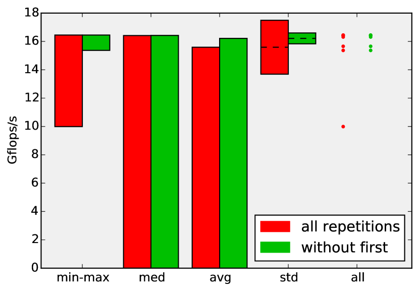
Figure 1: Performance statistics from 10 repetitions of dgemm
This second experiment produces ten measurements, from which we derive
statistics as those presented in Fig. 1. It is worth pointing
out that whenever multiple repetitions are executed and timed, the first one
almost inevitably represents an outlier; for the most part, this phenomenon is
connected to the initialization of the kernel library, but it is also due to
the loading and caching of data and instructions. In general, a more accurate
representation of the effective performance is obtained by dropping the first
measurement of the lot. In Fig. 1 one can appreciate how
significantly the first repetition affects the various statistics, and most
noticeably, the minimum, the average and the standard deviation (std).
In order to avoid the impact of “first-execution” outliers, in all following
examples and studies we always discard the measurement relative to the first
repetition.
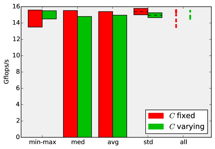
2.2 Data Placement: Varying Operands
In Experiment 2, the matrices , , and were reused across repetitions,
causing them to stay in cache; this scenario is also known as a “warm data”.
Depending on the application, the assumption of warm data may or may not be
realistic; to reflect this in our experiments, we allow to “vary” the
operands (i.e., use different memory locations) individually in each
repetition. Furthermore, in ELAPS one can freely control the relative
position of varying operands: They can be stacked horizontally or vertically,
with or without an arbitrary offset.
In the following experiment, while and are fixed and quite small,
varies in each repetition (hence the subscript in ) and is
therefore never cached (“cold data”).
In Fig. 2 we present the results of Experiment 3 and another
experiment in which the matrices , , and are all fixed. The
performance loss due to the enforced out-of-cache scenario for is clearly
visible.
2.3 Sequences of Kernels
In addition to isolated kernels, ELAPS allows to experiment with sequences of
calls. Let us use the solution of a linear system as an example: The problem
(1)
is typically solved by first LU-decomposing (dgetrf), and then by
solving two triangular linear systems (dtrsm). The process—which is
also implemented in LAPACK’s dgesv—is replicated in
Experiment 4.111For simplicity, we don’t expose the pivoting vector and omit the row
interchanging kernel dlaswp that only contributes a lower order term
to the execution time.
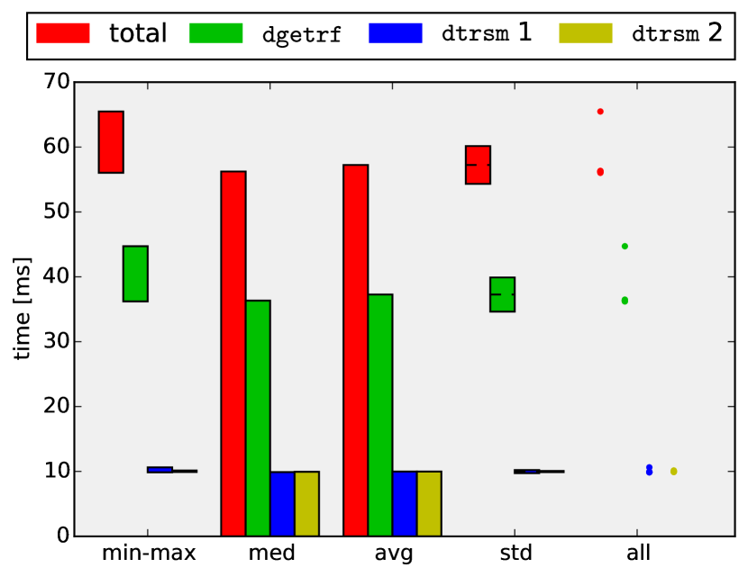
E5-2670OpenBLASExperiment 4: Linear System Breakdown⬇#threads=1repeat10times:dgetrf:dtrsm:dtrsm:
Figure 3: Breakdown of the timings for the solution of a linear system
For this experiment, Fig. 3 shows both the total execution time
and the time spent in each individual kernel. It is easy to realize that for
200 right-hand sides, the LU decomposition dgetrf is responsible for more
than of the total execution time, while each of the dtrsm’s
only contribute less than .
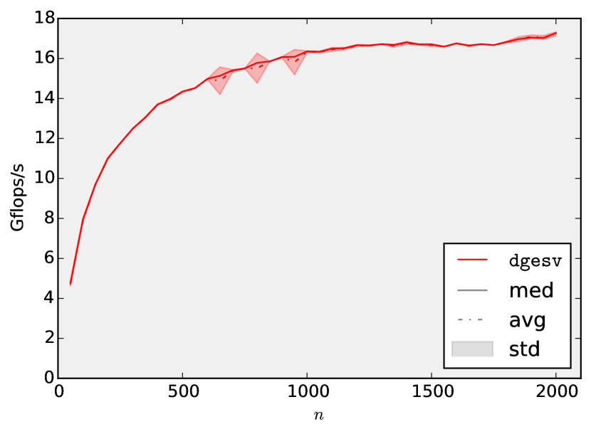
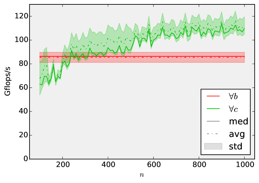
2.4 Parameter Range
So far we only considered experiments in which the sizes of the kernel operands
where fixed. In many practical experiments however one wants to study the
performance of a routine over a range of parameters. In the following example,
we use the routine dgesv, which solves a linear system directly, to solve
problems of size with right hand sides, where ranges from
to in steps of .
Figure 4: Solution of linear systems: performance.
Performance results from Experiment 5 are shown in Fig. 4; the
plot displays the increase in performance for increasing problem size, as
typical for dense linear algebra kernels.
2.4.1 Threads Range
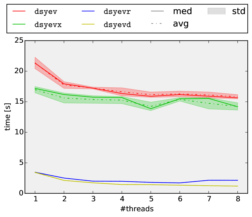
Scalability studies are extremely common examples of experiments that make use
of ranges. In the following experiments, we compute the eigenvalue
decomposition of a symmetric matrix (of fixed size) using from up to
threads, and compare LAPACK’s solvers dsyev, dsyevx, dsyevr, and dsyevd (see [1] for details on these routines).
Figure 5: Scalability of LAPACK’s symmetric dense eigensolvers on random matrices
As one can appreciate from Fig. 5, ELAPS makes it easy to
set up, execute, and compare the results of multiple experiments with varying
degrees of parallelism.
2.5 Sum- and OpenMP-Range
In loop-based algorithms, the total execution time is often more meaningful
than an iteration-by-iteration break-down. For this purpose, in addition to
the “parameter range” described in the previous subsection, ELAPS also
provides a “sum-range”, which yields the total contribution of the loop. For
instance, the next experiment models the inversion of a lower triangular
matrix222LAPACK’s dtrtri computes the inverse of a triangular matrix using a
similar algorithm.
of size via a blocked algorithm that traverses the matrix in steps
of a fixed block-size .
Figure 6: Influence of block-size on triangular inversion
2.5.1 OpenMP-Range
Fig. 6 reports the performance attained by this algorithm
for different block-sizes ; the maximum is observed for .
The choice of parameters represents an important step to tailor algorithms for
a given architecture; for instance, the tuning of the block size is common to
many of the algorithms included in LAPACK [22, 1]. Notice
that a simpler and finer-grained experiment to optimize the block-size is
obtained by combining the sum-range with a parameter-range for .
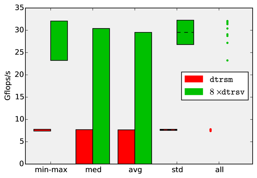
Multi-threading can typically be exploited in two different ways, namely,
either invoking a multi-threaded library (such as OpenBLAS), or through
OpenMP. To investigate these alternatives, in the Experiments 8 and 9 we
implement the solution of a triangular linear system with a tall and skinny
right-hand side 1) with OpenBLAS’s threaded dtrsm kernel, and 2) as
a series of parallel dtrsv’s666dtrsv: Linear system solve with a single right-hand side.
using ELAPS’s OpenMP-range.
E5-2670OpenBLASExperiment 8: Tall and skinny dtrsm⬇#threads=8repeat10times:dtrsm:
Figure 7: Performance of threaded dtrsm vs. parallel dtrsv’s
The results in Fig. 7 suggest that the parallel dtrsv’s are considerably faster than the threaded dtrsm’s, indicating
that OpenBLAS is not optimally parallelized for such extremely skewed
matrix sizes.
3 The ELAPS Framework
The ELAPS framework is built to support performance experiments combining the
features and scenarios described in Sec. 2. In this section,
we present the structure of the framework, focusing on the aspects that make it
general and intuitive, yet powerful.
Figure 8: Structure of the ELAPS framework
As shown in Fig. 8, ELAPS is structured in three layers.
•
The first, “bottom” layer (Sec. 3.1) is written in
C/C++ and contains the Sampler, a low-level command line tool
responsible for executing and timing individual kernels. The Sampler has to be compiled for each specific combination of hardware and
libraries (the only stage in which the user needs to configure the
system); ELAPS can interface with any number of Samplers.
•
The second, “middle” layer (Sec. 3.2) is the Python
library elaps, which centers around the class Experiment
that implements the previously introduced experiments. An Experiment can be executed on different Samplers, both locally or
through job submission systems. The outcome is a Report, which
provides not only structured access to the individual measurements, but
also functionality to analyze different metrics and statistics.
This layer also includes the plot module, which is based on the
matplotlib library, and is used to easily visualize Reports
in graphical form.777All the plots in this paper were generated in this manner.
•
The third, “top” layer (Sec. 3.3) adds a graphical user
interface, written in PyQt4, to both design Experiments in
the PlayMat and study Reports and plots in the Viewer.
The design of these three layers is discussed in the next subsections.
3.1 The Sampler
At the core of the ELAPS framework is a low-level performance measurement tool
tailored to dense linear algebra operations: the Sampler. This tool, earlier
versions of which were already utilized in [17] and
[18], makes it possible to measure the performance of individual
kernel executions, implementing this work-flow:
1.
Read from stdin a list of calls, i.e., kernel names with
corresponding lists of arguments;
2.
execute the specified calls, thereby measuring their performance in
terms of CPU cycles, and optionally through performance counters
provided by the Performance Application Programming Interface
(PAPI) [5];
3.
print the measured performance numbers to the standard output.
While reading the list of kernels from the standard input, the Sampler accepts
several special commands: go executes, measures, and reports the results
of all the calls previously read; {omp and } respectively start
and end a list of calls to be executed as parallel OpenMP tasks; set_counters sets the PAPI counters for the next set of executions.
The Sampler accepts kernels and arguments in a format that agrees with the
conventions used by standard libraries such as BLAS and LAPACK: Each argument
is passed by reference, and is of type char *, int *, float *, or double *.
In a dense linear algebra kernel, these arguments are of one of two types.
•
Scalar arguments point to scalar values, some of which may
influence the kernel’s behavior and control flow. Examples include:
flag arguments (e.g., side, transA), size arguments (e.g.,
m, n), scalars (e.g., alpha, beta), and leading
dimensions (e.g., ldA, ldB).
Within the Sampler, scalar argument values are stored consecutively in
an array.
•
Data arguments point to memory regions that hold the
mathematical objects (such as vectors or matrices) involved in the
kernel call. Generally888Eigensolvers are a notable exception.
, the actual contents of these arguments do not affect the control
flow; nonetheless, these arguments may still have a significant impact
on performance, depending on their location in the memory hierarchy.
The Sampler has two mechanisms to treat data arguments:
–
Named variables are designated memory regions
referenced by a variable names. A set of features to allocate
(xmalloc999 identifies the data-type.
), compute offsets (xoffset) and free (free)
such variables give users full control over where operands are
stored in relation to each other.
–
Dynamic memory offers a fast way to pass “unnamed”
memory regions as data arguments. Within one call all such
regions are guaranteed to be disjoint; across calls, however,
the same memory regions may be reused arbitrarily.
To set up the contents of data arguments, the Sampler provides a set
of simple utility-type kernels: xmemset fills every entry in
a buffer with a single value, xgerand fills it with random
values (uniform in ), and xporand generates a random
symmetric (or Hermitian) positive definite matrix. Furthermore,
xreadfile and xwritefile, read matrices from and
write them to binary files, respectively.
3.2 The elaps Package
The middle layer of the ELAPS framework centers around the experimental
features introduced in Sec. 2, encoded in the Python class
Experiment. Instances of this class form the starting point for
performance experiments; executing them using Samplers ultimately leads to
Reports, which can be analyzed with respect to a variety of metrics and
statistics.
3.2.1 Experiments
Experiment instances are both a static description of experiments, which
are easily stored to and loaded from strings and files for portability, but
also feature functionality to support their design and handling.
The kernel configurations at the center of each Experiment are its
connection to libraries such as BLAS or LAPACK. While the interfaces of such
libraries aim at being general by accommodating multiple functionalities,
precisely because of their generality they are often unintuitive and hard to
memorize. To counter this problem, elaps uses optional “Signatures” to annotate kernels, thereby providing possible value ranges and
semantic connections between arguments. In the end, these Signatures
allow Experiments to expose feasible values for arguments (such as trans or uplo) and automatically derive connected arguments such as
operand sizes and leading dimensions, both within a single kernel and across
multiple kernels.
The execution of an Experiment is initiated by the submit method.
This method first generates the sequence of kernel calls for the Sampler and a
shell script for its execution; it then either executes this script is locally
or submits it to a batch job system.
3.2.2 Execution on Samplers
In this section, we describe how the Experiment features are translated
into commands for the Sampler.
As input, the Sampler expects a raw list of kernel invocations. To produce
this list, all ranges and repetitions in an Experiment are completely
unrolled, thereby evaluating any symbolic (range-dependent) variable. The OpenMP-range is translated directly to the Sampler’s {omp and }
commands. Using the parameter-range to vary the number of library threads
requires to interface with said library; to avoid library-dependent kernels
and Sampler features, we do so through environment variables (e.g., OPENBLAS_NUM_THREADS) and by starting the sampler separately for each thread
count.
Data arguments in kernels are allocated as named variables in the Sampler at
the beginning of the input. Arguments that vary with repetitions or the
sum/OpenMP-range (i.e., they point to different locations) are first
allocated as a single large block and then subdivided by calculating
appropriate offsets, resulting in individual variables for each repetition and
range iteration.
Finally, PAPI counters are also set at the beginning through the set_counters command.
3.2.3 Reports
Each Experiment execution results in a report file that, when read into
elaps, turns into a Report instance. This object serves as a
structured representation of the obtained measurements with respect to the
underlying Experiement: Raw measurements are accessed through the
hierarchy “parameter-range value repetition
sum/OpenMP-range value kernel” and yield the cycle count
or PAPI counter measurements. Separately, a “reduced” view on the results
accumulates the sum/OpenMP-range and the kernels according to the
experiment semantic.
To turn these structured yet raw measurement results into more meaningful
quantities, metrics combine them with the kernels’ flop counts and
information on the their execution environment. The easily extensible set of
metrics ranges from “execution time in seconds” to “” and
“efficiency”.
While a metric converts measurements values one-by-one, results from multiple
repetitions are combined by statistics, such as “minimum”, “maximum”,
“median” or “standard deviation”. As motivated in
Sec. 2, the results from first repetitions are optionally
discarded to hide overhead effects and make statistics more representative of
in-application invocations.
3.2.4 Plotting
ELAPS’s plot module generates matplotlib figures from the
structured data in Reports under consideration of both metrics and
statistics. Depending on the type of experiment, it automatically generates
appropriate bar- or line-plots that are easily exported to various file
formats.
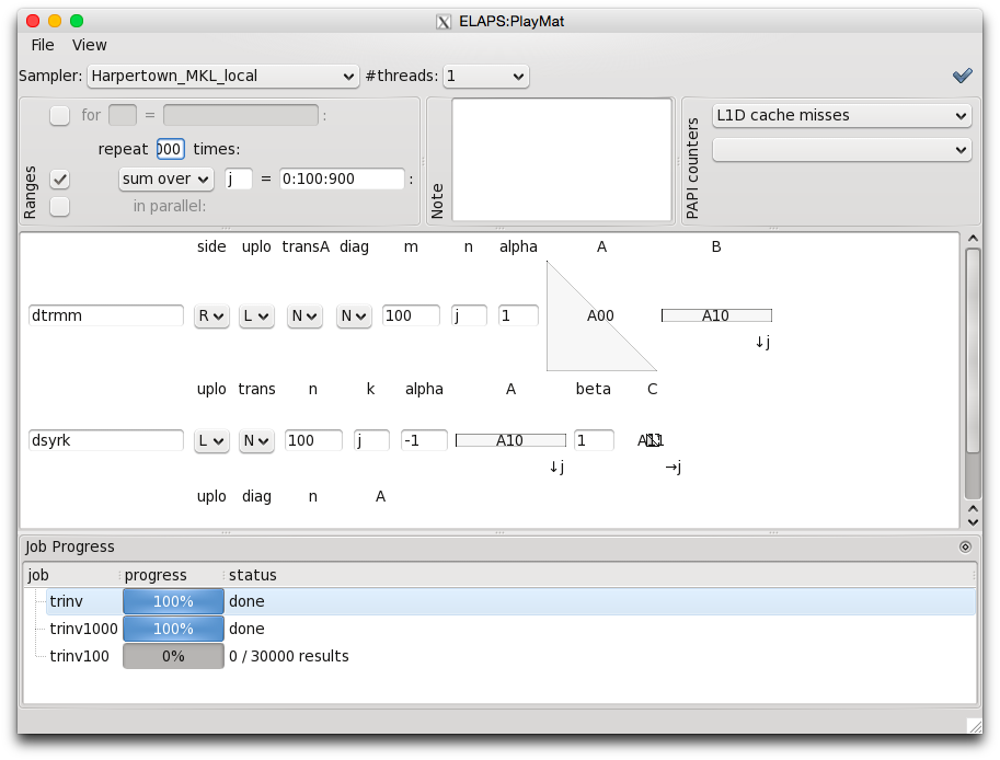
3.3 The Graphical User Interface
ELAPS’s Experiment and Report Python classes establish a flexible
and powerful foundation for performance evaluations at a scripting level. In
order to enable performance experimentation in an explorative fashion, and to
facility more intuitive interaction, ELAPS features a graphical user
interface. As shown in Fig. 8, this interface consists of
components: While the PlayMat serves as a “playing mat” to develop Experiments, the Viewer interactively visualizes Reports.
Figure 9: The PlayMat through X11.
The PlayMat, shown in Fig. 9, allows interactive access to the
full functionality of an Experiment. To further guide the user, among
other things, it visualizes the Experiment’s kernels based on their Signatures similar to how they are presented in this paper and automatically
calculates matrix sizes and (if desired) deducible arguments, such as leading
dimensions. It furthermore provides progress tracking of executing Experiments and can load completed Reports directly in the Viewer.
Figure 10: The Viewer on Mac OS X
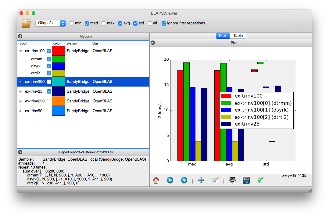
The Viewer, shown in Fig. 10, is an interactive means to analyze
and compare Reports. It provides all metrics applicable to the selected
Reports and its statistical plots are easily manipulated and exported.
4 Application Examples
In this section, we demonstrate the use of the ELAPS framework in several
application examples. For this purpose, we deliberately chose a wide range of
hardware systems and kernel libraries.
4.1 Algorithm Selection: Tensor Contractions
Let us consider the tensor contraction (in Einstein notation)
(2)
with
,
, and
, where is between
and . Using an explicit index notation, is computed as
(3)
and can be visualized as follows:
()
()
A natural approach to efficiently compute such tensor contractions is to
utilize the highly optimized dgemm kernel. For Contraction
(2), there are two ways of casting the computation as a series
of dgemm’s:
(4)
(5)
An inspection of these algorithms reveals that they both execute a dgemm
of fixed size on varying data; in particular, the number of invocations in
Algs. and are, respectively, and . By
virtue of this observation, Experiments 10 and 11 only perform
repetitions, thus reducing the experimentation time; while the results will not
be meaningful estimates for the total execution time, they will expose the same
computational efficiency (expressed in ) as the full algorithms.
Furthermore, since Alg. operates on matrices of fixed size and
independent of , in Experiment 10 we also avoid the use of the parameter
range.
We perform Experiments 10 and 11 on a 16-core IBM PowerPC A2 node of the
IBM BlueGene installation JUQUEEN at the Jülich Supercomputing
Center, linked to IBM’s optimized ESSL library. Only the Sampler is executed
on this compute node, running the lightweight CNK operating system; it is
accessed by elaps from a Red Hat Enterprise Linux 6.6 front-end
node through the LoadLeveler batch job system.
Figure 11: Comparison of dgemm-based algorithms for tensor contraction
2
Fig. 11 suggests that neither of the two algorithms is optimal
for all cases: While for a small dimension , algorithm is
better, algorithm dominates for large . Interestingly, the
crossover point is not at , where both algorithms work with
matrices of equal size, but already around .
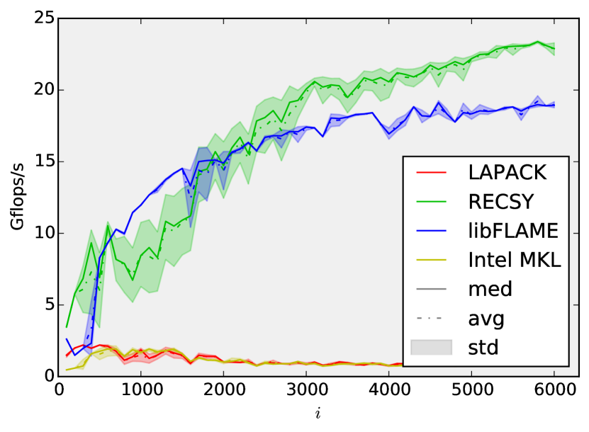
4.2 Library Selection: Sylvester Equation
Choosing the right library can be a crucial step in attaining high performance.
In this section, we demonstrate its importance by considering the triangular
Sylvester equation
(6)
to be solved for , which is central to problems in control theory. In
addition to LAPACK’s dtrsyl, several other libraries offer this kernel
with the same interface. In our tests, we consider
libFLAME101010While libFLAME’s LAPACK interface does by default not call
its optimized Sylvester solver, it is easily exposed.
5.1.0-18 [21] linked to OpenBLAS, and
To compare these libraries, we launch Experiment 12 on a 10-core Intel
IvyBridge E5-2680 v2 processor with Samplers linked to the above libraries.
This machine, which is part of a compute cluster is accessed through the Platform LSF 9.1.2 batch job system with both the front-end (elaps) and
back-end (the Samplers) running Scientific Linux 6.6.
Figure 12: Comparison of libraries for the triangular Sylvester equation
Fig. 12 shows the performance attained by the different libraries.
LAPACK, which only provides an unblocked algorithm for dtrsyl, reaches
for small problems but eventually falls below
. The specialized RECSY library on the other hand attains the
best performance of up to . libFLAME is initially
competitive with RECSY but eventually tops at .
Surprisingly, the otherwise very efficient MKL seems poorly optimized for this
problem and is as fast as LAPACK.
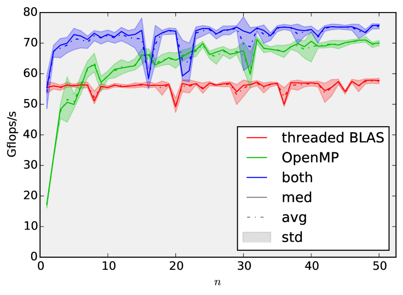
4.3 Multithreading: Sequence of LUs
In a certain type of electronic structure calculations [2], one has to
solve a series of fairly small linear systems. As already mentioned, a possible
approach involves the LU factorization (dgetrf) and two triangular linear
systems (dtrsm) for each matrix; since each system only involves two
right-hand sides, the cost for the dtrsm’s is entirely negligible.
On multi-core machines, the sequence of LUs can be parallelized at the
granularity of one matrix, via a multi-threaded dgetrf kernel, or by
assigning different matrices to different threads, via OpenMP (hybrid
solutions are also possible). Performance-wise, there are arguments both in
favor and against each of these two alternatives: Using BLAS’s internal
parallelism ensures that only one kernel uses the CPU’s caches at a time; on
the other hand, OpenMP’s parallelism increases the amount of work that
the CPU’s cores can perform simultaneously.
The next three experiments use ELAPS’s sum-range and OpenMP-range
constructs to model the scenarios in which 1) a multi-threaded kernel is used,
2) OpenMP runs sequential kernels in parallel, and 3) OpenMP runs
multi-threaded kernels in parallel.111111This third experiment is not
displayed: It is obtained from Experiment 14, changing #threads to 8.
Each of them measures the time it takes to LU decompose an increasing number of
square matrices of size .
These three experiments are executed on a MacBook Pro running OS X 10.9.4
with a quad-core Intel Haswell i7-4850HQ CPU (Turbo Boost disabled) using
Apple’s Accelerate framework; both the Sampler and elaps run
on the same platform.
Figure 13: Multi-threading paradigms for a sequence of
LUs131313
Even though the Turbo Boost was disabled and no other
application was running,
noticeable performance fluctuations were observed.
This is to be expected on laptop-systems.
footnote 13 indicates that of the two “pure” approaches, if more than
LU’s are performed (i.e., more than the CPU has hardware threads), OpenMP with single-threaded kernels outperforms Accelerate’s parallel
kernel. However, the mixed approach, in which Accelerate uses up to
threads, while OpenMP is allowed to schedule the LU decomposition
tasks, is even more efficient, reaching up to .
4.4 Algorithmic Optimization: GWAS
Genome Wide Association Studies (GWAS) investigate how human traits (e.g. eye
color or genetic deceases) are related to certain locations in the human
genome [4, 24]. Computationally, GWAS can be cast as a sequence of
Generalized Least Squares (GLS) problems
(7)
where is symmetric positive definite, , , and with
, and ,
where can be in the millions.
A straightforward implementation of this equation (e.g., using R or Matlab)
might compute each individually by solving Equation 7 from right
to left, as modeled in this next experiment (with and ):
Xeon PhiMKLExperiment 15: Multiple GLS⬇#threads=240for=100:100:1000:sumover=1::dposv141414dposv: Cholesky decomposition + linear system solve.
:dgemv151515dgemv: General matrix vector product.
:dpotrs161616dpotrs: Linear system solve following a Cholesky decomposition.
:dsyrk:dposv:
For Experiments 15 and 16, we choose a 60-core Intel Xeon Phi
co-processor using Intel MKL. ELAPS’s python library and the PlayMat are run on this system’s Host processor (Scientific Linux 6.6); only the
Sampler is executed natively on the co-processor.
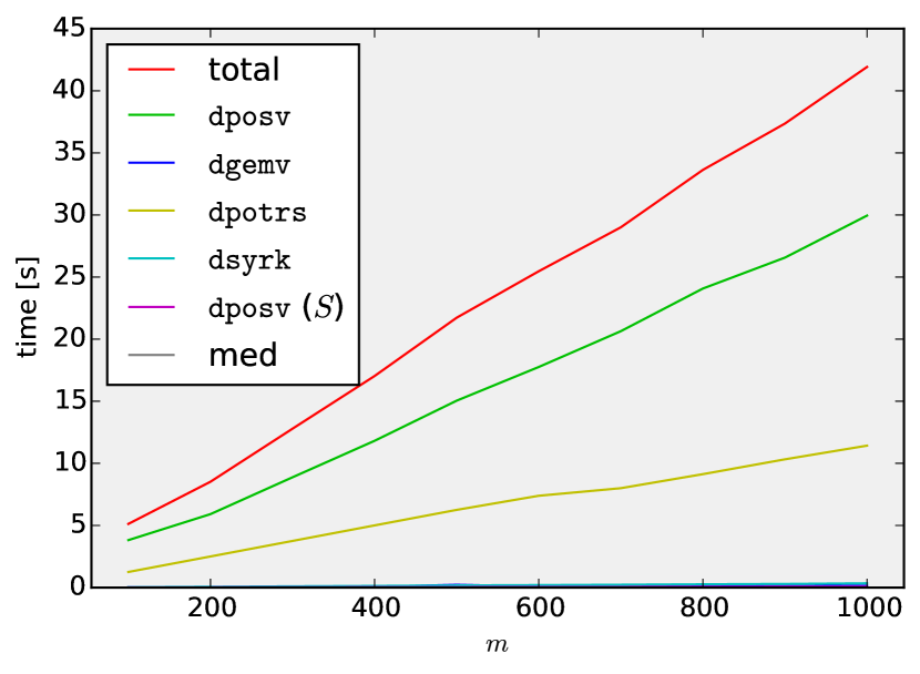
Figure 14: Timing breakdown for a sequence of GLS solves
Fig. 14 shows both the execution time of Experiment 14, as well as a
breakdown thereof. The runtime is clearly dominated by the dposv and dpotrs kernels involving .
From a first analysis of these two kernels, one realizes that the dposv
() is independent of , and can thus be taken out of
the loop and computed just once. This modification reduces dposv’s
contribution to the total runtime by a factor of , effectively shifting the
bottleneck onto dpotrs.
A further analysis reveals that all the dpotrs linear systems involve the
same matrix ; this observation suggests to combine the right-hand sides for all iterations into a single large
matrix . The following
experiment solves a linear system with this matrix as the right-hand side with
a single invocation of dpotrs:
For the selected range of , the runtime of this experiment is below
, i.e., already more than 1 order of magnitude less than the
previous experiment. Furthermore, for larger problems, the dpotrs kernel
can make good use of the co-processor’s many cores and reaches over
. For an in depth study of performance optimizations for
GWAS we refer the reader to [smp-gwas] and [9].
5 Conclusion
We introduced the Experimental Linear Algebra Performance Studies framework
(ELAPS), a set of tools and features to design, execute, measure and analyze
dense linear algebra performance experiments. With its intuitive interface,
ELAPS assists users in investigating performance behaviors and in making
informed decisions. Throughout this paper, we applied ELAPS to a wide range
of scenarios, including parameter optimization (Sec. 2.5),
algorithm selection (Sec. 2.4.1, Sec. 4.1), library
comparison (Sec. 4.2), and parallelism and library threading
(Sec. 2.5.1, Sec. 4.3). We demonstrated the
framework’s flexibility by linking it with seven kernel-libraries, and by
executing experiments on five different platforms, including the Xeon Phi
co-processor and two different batch-job systems. In summary, ELAPS covers
many aspects of shared-memory optimizations, a critical step towards achieving
large-scale performance.
Having established the foundations of a framework for rapid experimentation, we
foresee many opportunities for extensions. In particular, we envision 1)
coverage of a broader range of architectures, including GPUs and ARM-based
CPUs, 2) support for metrics related to data movement and energy consumption,
and 3) interfaces for distributed memory libraries such as ScaLAPACK.
Financial support from the Deutsche Forschungsgemeinschaft (DFG) through
grant GSC 111 and from the Deutsche Telekom Stiftung, and access to JUQUEEN
at Jülich Supercomputing Centre (JSC) are gratefully acknowledged.
References
[1]
E. Anderson, Z. Bai, C. Bischof, S. Blackford, J. Demmel, J. Dongarra,
J. Du Croz, A. Greenbaum, S. Hammarling, A. McKenney, and D. Sorensen.
LAPACK Users’ Guide.
Society for Industrial and Applied Mathematics, Philadelphia, PA,
third edition, 1999.
[2]
D. S. G. Bauer and S. Blügel.
Development of a relativistic full-potential first-principles
multiple scattering Green function method applied to complex magnetic
textures of nano structures at surfaces.
PhD thesis, Jülich, 2013.
Druck-Ausgabe: 2013. - Online-Ausgabe: 2014; Zugl.: Aachen, Techn.
Hochsch., Diss., 2013.
[3]
P. Bientinesi, B. Gunter, and R. van de Geijn.
Families of algorithms related to the inversion of a symmetric
positive definite matrix.
ACM Transactions on Mathematical Software, 35(1), July 2008.
[4]
E. Boerwinkle, R. Chakraborty, and C. F. Sing.
The use of measured genotype information in the analysis of
quantitative phenotypes in man. I. Models and analytical methods.
Ann. Hum. Genet., 50(Pt 2):181–194, May 1986.
[5]
S. Browne, J. Dongarra, N. Garner, G. Ho, and P. Mucci.
A portable programming interface for performance evaluation on modern
processors.
Int. J. High Perform. Comput. Appl., 14(3):189–204, Aug. 2000.
[6]
R. S. Chen and J. K. Hollingsworth.
Towards fully automatic auto-tuning: Leveraging language features of
chapel.
Int. J. High Perform. Comput. Appl., 27(4):394–402, Nov. 2013.
[7]
C. Ţăpuş, I.-H. Chung, and J. K. Hollingsworth.
Active harmony: Towards automated performance tuning.
In Proceedings of the 2002 ACM/IEEE Conference on
Supercomputing, SC ’02, pages 1–11, Los Alamitos, CA, USA, 2002. IEEE
Computer Society Press.
[8]
J. W. Demmel, O. A. Marques, B. N. Parlett, and C. Vömel.
Performance and accuracy of lapack’s symmetric tridiagonal
eigensolvers.
SIAM J. Sci. Comput., 30(3):1508–1526, Mar. 2008.
[9]
D. Fabregat-Traver and P. Bientinesi.
Computing petaflops over terabytes of data: The case of genome-wide
association studies.
ACM Transactions on Mathematical Software (TOMS), 40(4):Article
27, June 2014.
[10]
M. Frigo and S. G. Johnson.
The design and implementation of FFTW3.
Proceedings of the IEEE, 93(2):216–231, 2005.
Special issue on “Program Generation, Optimization, and Platform
Adaptation”.
[11]
M. Geimer, F. Wolf, B. J. N. Wylie, E. Ábrahám, D. Becker, and B. Mohr.
The scalasca performance toolset architecture.
Concurr. Comput. : Pract. Exper., 22(6):702–719, Apr. 2010.
[12]
A. Hurault, K. Baek, and H. Casanova.
Selecting linear algebra kernel composition using response time
prediction.
Software: Practice and Experience, pages n/a–n/a, 2014.
[13]
Intel.
Math kernel library.
[14]
I. Jonsson and B. Kågström.
Recsy – a high performance library for sylvester-type matrix
equations.
In H. Kosch, L. Böszörményi, and H. Hellwagner, editors, Euro-Par 2003 Parallel Processing, volume 2790 of Lecture Notes in
Computer Science, pages 810–819. Springer Berlin Heidelberg, 2003.
[15]
W. E. Nagel, A. Arnold, M. Weber, H.-C. Hoppe, and K. Solchenbach.
Vampir: Visualization and analysis of mpi resources.
Supercomputer, 12:69–80, 1996.
[17]
E. Peise and P. Bientinesi.
Performance modeling for dense linear algebra.
In Proceedings of the 2012 SC Companion: High Performance
Computing, Networking Storage and Analysis (PMBS12), SCC ’12, pages
406–416, Washington, DC, USA, Nov. 2012. IEEE Computer Society.
[18]
E. Peise, D. Fabregat-Traver, and P. Bientinesi.
On the performance prediction of blas-based tensor contractions.
In Proceedings of the 5th International Workshop on Performance
Modeling, Benchmarking and Simulation of High Performance Computer Systems
(PMBS14), Nov. 2014.
[19]
C. Schaefer, V. Pankratius, and W. Tichy.
Atune-il: An instrumentation language for auto-tuning parallel
applications.
In H. Sips, D. Epema, and H.-X. Lin, editors, Euro-Par 2009
Parallel Processing, volume 5704 of Lecture Notes in Computer Science,
pages 9–20. Springer Berlin Heidelberg, 2009.
[20]
S. S. Shende and A. D. Malony.
The tau parallel performance system.
Int. J. High Perform. Comput. Appl., 20(2):287–311, May 2006.
[21]
F. G. Van Zee.
libflame: The Complete Reference.
lulu.com, 2009.
[22]
R. Whaley.
Empirically tuning lapack’s blocking factor for increased
performance.
In Computer Science and Information Technology, 2008. IMCSIT
2008. International Multiconference on, pages 303–310, Oct. 2008.
[23]
R. C. Whaley and J. J. Dongarra.
Automatically tuned linear algebra software.
In Proceedings of the 1998 ACM/IEEE Conference on
Supercomputing, SC ’98, pages 1–27, Washington, DC, USA, 1998. IEEE
Computer Society.
[24]
J. Yu, G. Pressoir, W. H. Briggs, I. Vroh Bi, M. Yamasaki, J. F. Doebley, M. D.
McMullen, B. S. Gaut, D. M. Nielsen, J. B. Holland, S. Kresovich, and E. S.
Buckler.
A unified mixed-model method for association mapping that accounts
for multiple levels of relatedness.
Nat. Genet., 38(2):203–208, Feb 2006.