Tree-Grass interactions dynamics and Pulse Fires: mathematical and numerical studies

Abstract

Savannas are dynamical systems where grasses and trees can either dominate or coexist. Fires are known to be central in the functioning of the savanna biome though their characteristics are expected to vary along the rainfall gradients as observed in Sub-Saharan Africa. In this paper, we model the tree-grass dynamics using impulsive differential equations that consider fires as discrete events. This framework allows us to carry out a comprehensive qualitative mathematical analysis that revealed more diverse possible outcomes than the analogous continuous model. We investigated local and global properties of the equilibria and show that various states exist for the physiognomy of vegetation. Though several abrupt shifts between vegetation states appeared determined by fire periodicity, we showed that direct shading of grasses by trees is also an influential process embodied in the model by a competition parameter leading to bifurcations. Relying on a suitable nonstandard finite difference scheme, we carried out numerical simulations in reference to three main climatic zones as observable in Central Africa.

Keywords: Savanna; tree/grass competition; ecological gradients ; fires; periodic solutions; stability; impulsive differential equations (IDE); bifurcation; nonstandard finite difference scheme.

MSC Classification: Primary 30A37, 92D40. Secondary: 37M05

1 Introduction

In savannas, trees and grasses typically coexist [1]. Fire is recognized as playing a major part in the dynamics of this biome. The nature of grass-tree interactions and fire regimes strongly vary along environmental gradients in tropical savannas. Fire is more intense in wet than in arid savannas, where lower water availability leads to lower grass, i.e. fuel load, production. Thus fire is expected to control Tree-Grass dynamics in wet savannas [2]. But two hypotheses for Tree-Grass coexistence have been introduced during these last decades. First, Walter (1971) [3] proposed the idea that trees and grass exploit two different rooting niches. Grasses are rooted in superficial soil layers and first use the incoming water, whereas tree roots are situated in subsoil, so that trees could grow only where enough water reached deeper soil horizons. This idea was developed analytically by Walker and Noy-Meir (1982) [4] using a Lotka-Volterra theory of co-existence between competitors. The second hypothesis says that grass-tree coexistence is driven by limited opportunities for seedling to escape both droughts and flame zone into the adult stage (Hochberg et al. 1994 [5]; Higgins et al. (2000) [6]). In areas where tree seedlings succeed to establish in spite of competition with grasses, they are burnt by frequent grass fires (Higgins et al. 2000 [6]).

Savannas fires are frequent, up to occurring every 1-5 years in wet savannas (Frost & Robertson 1985) though the fire return time is usually a decreasing function of mean annual precipitation. Fuel load made of dead aerial grass parts typically ranges between $2$ and $10$ t.ha^-1 of dry matter (DM) (Lacey et al. 1982 [7]; Stronach & Mac-Naughton 1989 [8]; Menaut et al. 1991 [9]; Mordelet 1993 [10]) and flame height is usually $2$-$3$ metres high (Frost & Robertson 1987 [11]). Although the fire burns most or all the aboveground grass biomass, the large underground root systems of perennial grass species enable most of the tufts to survive even the most intense fires and to rapidly establish new shoots before the onset of the rainy season. In contrast to grasses, trees which are less than $2$m height may either succumb to fire or have to resprout from roots and have their growth delayed (Bond and Midgley, 2001 [12]). Mature trees ($>8$m) and shrubs beyond $2$m are more fire resistant and only experience partial die-back (Menaut & C sar 1979 [13]; Gillon 1983 [14]). Early fires (in the beginning of the dry season) are less violent than late fires and have a lower impact on tree regeneration (Abbadie et al. 2006 [15]).

Africa is a land of extreme contrasts in rainfall distribution and the time of year during which rainfall occurs (Janowiak 1987 [16]). When soil resource supply is temporally variable, trees and grasses will experience two distinct phases of resource availability: pulse periods when resources are high and most growth and biomass accumulation (fuel load) occurs, and inter-pulse periods when resources are too low for most tree and grass to take up and most mortality due to resource deficits takes place (Goldberg & Novoplansky, 1997 [17]; Noy-Meir, 1973 [18]). Hence essential resource availability (e.g. water) is discontinuously available and the availability of these resources impact the ecosystem as discrete pulse events interspersed among long periods of limited resource availability (Schwinning et al. 2004 [19]).

Fires are sudden event that consume trees and grass biomass (Scheiter 2008 [20]). The broad objective of this study is to examine the influence of pulse events with regard to fires impact on the Tree-Grass dynamics along the rainfall gradient in Africa. Tree-grass savanna models can not be studied without the important role of fires (Tilman 1994 [21]; Higgins et al. 2000 [22]; Sankaran et al. 2004 [23], 2005 [24]; D’Odorico et al. 2006 [25]; Accatino et al. 2010 [26]; Beckage et al. 2011 [27]; Staver et al. 2011 [28]; Yatat et al. 2014 [29] and Tchuinte et al. 2014 [30]). This paper extends our earlier work (Tchuinte et al. 2014 [30]) where we consider a continuous tree-grass interaction model that featured a fairly generic family of non-linear functions of grass biomass to model fire intensity and its impact on tree. We have shown that the continuous model is able to predict a variety of dynamical outcomes. Notably, the number of equilibria featuring Tree-Grass coexistence depends on the characteristics of fairly generic Monod functions used to model the fire impact on tree dynamics. Moreover, we have shown that various bistability situations occur among forest, grassland and Tree-Grass (i.e. savanna) equilibria (for more detail see Tchuinte et al. 2014 [30]). Of course, in practice, fires are not continuous. Recent studies of the interactions between fire and vegetation are based on stochastic approaches because of the random and unpredictable nature of fire occurrences (D’Odorico et al., 2006 [25]; Beckage et al. 2011 [27]).

In section 2 we will present the model with pulse fires. The theoretical analysis is developed in section 3. We show that the system admits four equilibria among which two trivial equilibria (the bare soil and the forest equilibria), and two periodic equilibria (the periodic grassland and the periodic savanna equilibria). We show that there are various bistabilities: between forest and grassland; between forest and savanna. Local and global stabilities are distinguished using classical tools such as Floquet multipliers and comparison theorem. We highlight thresholds that summarize the dynamics of the model and explain the theoretical meaning of these thresholds. Prior to illustrate our theoretical results numerically, in section 4, based on the scheme developed in [29], we develop a reliable nonstandard finite difference method (NSFD) that preserves the qualitative properties of the system (Anguelov et al. 2012 [31], 2013 [32], 2014 [33]). Section 6 concludes the paper. Some mathematical details are included in appendices.

2 The mathematical model

In savanna environment, fire intensity is tightly linked to dried grass biomass that remains during the dry season (Higgins et al. 2008 [22]). During the last decades the effects of fire on vegetation dynamics have been studied (Scholes and Walker 1993 [34]; Higgins et al. 2000 [6]). Most of the models associated to or derived from these studies are ordinary differential equations (ODE) which assume that fires occur continuously with a fixed frequency. However fires are sudden event that consume grass biomasses and kill or harm tree seedlings (Scheiter 2008 [20]). The season of burning and the time between recurring fires determine trees and grass physioniomies in most ecosystems and especially in the savanna biome (Thonicke et al., (2001) [35]). In this paper we present a new Tree-Grass model that aim to contribute to our understanding about how pulse fire shapes vegetation dynamics in fire-prone savanna-like ecosystems. We consider fire as discrete events and derive the following impulsive differential system

$$\left\{\begin{array}[]{l}\left.\begin{array}[]{l}\displaystyle\frac{dG}{dt}=\gamma_{G}G\left(1-\displaystyle\frac{G}{K_{G}}\right)-\delta_{G0}G-\gamma_{TG}TG,\\ \\ \displaystyle\frac{dT}{dt}=\gamma_{T}T\left(1-\displaystyle\frac{T}{K_{T}}\right)-\delta_{T}T,\\ \end{array}\right\},t\neq t_{n},n=1,2,...,N_{\tau}\\ \left.\begin{array}[]{l}\\ \Delta G(t_{n})=G(t_{n}^{+})-G(t_{n})=-\lambda_{fG}G(t_{n}),\\ \\ \Delta T(t_{n})=T(t_{n}^{+})-T(t_{n})=-\lambda_{fT}\omega(\lambda_{fG}G(t_{n}))T(t_{n}),\\ \end{array}\right\},t=t_{n},n=1,2,...,N_{\tau}\\ \\ G(t_{0}^{+})=G_{0},\\ \\ T(t_{0}^{+})=T_{0},\end{array}\right.$$ (1)

where,

• $T$ and $G$ are tree and grass biomasses respectively,

• $\tau=\frac{1}{f}$ is the period of time between two consecutive fires, and $f$ is the frequency of fire,

• $N_{\tau}$ is a countable number of fire occurrence,

• $t_{n}=n\tau,$ $n=1,2,...,N_{\tau}$ are called moments of impulsive effects of fire, and satisfy $0\leq t_{1}<t_{2}<...<t_{k}<t_{N_{\tau}}$ ,

• $\omega(G)$ is a generic non-linear functional which expresses fire intensity as an increasing function of grass biomass. Other than smoothness, it satisfies the following three conditions: $(i)$ fires spread if and only if fuel is available ($\omega(0)=0$), $(ii)$ fire-impact increases with fuel available ($\omega(G)\geq 0$, $\omega^{{}^{\prime}}(G)>0$), and $(iii)$ there is boundary effects $\lim\limits_{G\rightarrow\infty}\omega(G)<1$.

Other parameters used are listed in the following table.

Table 1: Parameter symbols and names used to initialize the model

Symbol	Parameter name	Units
$\gamma_{G}$	Grass biomass production per unit of grass biomass per year	yr-1
$\delta_{G0}$	Grass biomass loss by herbivory (grazing) or human action	yr-1
$K_{G}$	Carrying capacity of grass biomass	t.ha-1
$\mu_{G}=\displaystyle\frac{\gamma_{G}}{K_{G}}$	Additional death due to grass-grass competition	ha.t-1.yr-1
$\lambda_{fG}$	loss of grass biomass due to fire	-
$\gamma_{T}$	Tree biomass production per unit of tree biomass per year	yr-1
$\delta_{T}$	Tree biomass loss by herbivory (browsing) or human action	yr-1
$K_{T}$	Carrying capacity of tree biomass	t.ha-1
$\mu_{T}=\displaystyle\frac{\gamma_{T}}{K_{T}}$	Additional death due to tree-tree competition	ha.t-1.yr-1
$\lambda_{fT}$	loss of tree biomass due to fire	-
$\gamma_{TG}$	grass mortality due to tree/grass competition	ha.t-1.yr-1

We suppose that solutions of $(\ref{Impuleq1})$ is right continuous at $t_{n}$, $n=1,2,...,N_{\tau}$, that is $G(t_{n}^{+})=\lim\limits_{h\rightarrow 0^{+}}G(t_{n}+h)=G(t_{n})$ and $T(t_{n}^{+})=\lim\limits_{h\rightarrow 0^{+}}T(t_{n}+h)=T(t_{n})$, where $G(t_{n}^{+})$ and $T(t_{n}^{+})$ are the biomass values for grasses and trees instantly after impulsive fire. Immediately following each fire pulse, system (1) evolves from its new initial state without being further affected by the fire scheme until the next pulse is applied. In agreement with empirical experience (Abbadie et al., 2006 [15]), we assume that the level of destruction of the tree biomass depends on the available grass biomass through $\omega(G)$.

3 Theoretical analysis

System (1) belongs to basic theory of IDE (Bainov 1993 [36]) and their applications in Ecology. IDEs generally describe phenomena which are subject to abrupt or instantaneous changes. Model (1) derives from the family of impulsive Kolmogorov-type population dynamics in the theory of mathematical biology which the general form is given by

$$\left\{\begin{array}[]{l}\displaystyle\frac{dx}{dt}=x_{i}(t)f_{i}(t,x(t)),\hskip 2.84544ptt\neq t_{k},\\ x_{i}(t_{k}^{+})=I_{ik}(t_{k},x(t_{k})),\hskip 2.84544ptt=t_{k}\end{array}\right.$$ (2)

where $x_{i}(t)$ represents the density or size of species $x_{i}$ at the time $t$, $x(t)=(x_{1}(t),x_{2}(t),...,x_{n}(t))$, $f(t,x)$ is an n-dimensional real functional defined by

$$f(t,x)=(f_{1}(t,x),f_{2}(t,x),...,f_{n}(t,x))$$

and $I_{k}(t_{k},x)$ is also an n-dimensional real functional defined by

$$I_{k}(t_{k},x)=(I_{1k}(t_{k},x),I_{2k}(t_{k},x),...,I_{nk}(t_{k},x)).$$

This family of models has recently attracted the attention of several authors ([37], [38], [39], [40], [41], [42], [43], and the references cited therein). The main study subjects are the permanence, persistence and extinction of species, the local and global asymptotic stability of systems, the existence and uniqueness of positive periodic solution and almost periodic solution, and the bifurcation and dynamical complexity, etc. However, in all models investigated in the literature, authors generally do not consider the non-linear impulses i.e. non-linear form of the function $I_{k}(t_{k},x)$. They mostly focused on the quasi-linear impulses. Since for the continuous model (see Tchuinte et al. 2014 [30]) the non-linear shape brings a wealth of possibilities, notably for the existence of various positive Tree-Grass equilibria. We retain this option although it could render the model difficult to study. In our model, we consider a generic non-linear functional response $\omega(G)$, which expresses the causality between grass biomass and fire intensity as to model the impact of fire on the woody biomass. Depending of the fuel accumulation (grass biomass i.e. G), $\omega(G)$ could take the general sigmoidal form $\displaystyle\frac{G^{\theta}}{\alpha^{\theta}+G^{\theta}}$, $\theta>0$, or some equivalent form. However, in our study $\omega(G)$ is principally treated as a non-linear increasing function. In this regard, since our Tree-Grass model does not contain more than two populations in competition, it may appear to be simple mathematically at first sight, but it is, in fact very challenging and complicated due to the nonlinear impulsive functions.

Prior to analyzing the above model $(\ref{Impuleq1})$, it is important to show positivity and boundedness for solutions as they represent biomasses. Positivity implies that the populations survive and boundedness may be interpreted as a natural restriction to growth as a consequence of limited resources. Then, model $(\ref{Impuleq1})$ requires that trajectories remain positive and that trajectories do not tend to infinity with increasing time.

Set $X_{G}=\displaystyle\frac{r_{G}}{\mu_{G}}$ and $Y_{T}=\displaystyle\frac{r_{T}}{\mu_{T}}$, where $r_{G}=\gamma_{G}-\delta_{G0}$ and $r_{T}=\gamma_{T}-\delta_{T}$ are net primary production of grass and tree biomasses respectively. The following lemma holds.

Lemma 3.1

When $\gamma_{G}>\delta_{G0}$ and $\gamma_{T}>\delta_{T}$, the compact

$$\mathcal{B}=\left\{(G,T)^{T}\in\mathbf{R}_{+}^{2}/G\leq X_{G}=K_{G}\left(1-\displaystyle\frac{\delta_{G0}}{\gamma_{G}}\right),T\leq Y_{T}=K_{T}\left(1-\displaystyle\frac{\delta_{T}}{\gamma_{T}}\right)\right\}$$

is positively invariant and attracting for the system (1). Note that solutions of system (1) are bounded below by 0, and above by the carrying capacities of grass and tree biomasses.

Proof: See appendix A, page Appendix A: Proof of Lemma 3.1.

When $t\neq n\tau$, the right-hand side of system (1) is locally Lipschitz continuous on $\mathcal{B}$. Thus, system (1) has a unique solution.

3.1 Equilibria

System (1) has constant and periodic equilibria.
First of all, it is obvious that $E_{00}=(0;0)$ and $E_{01}=(0,Y_{T})$ are "trivial" equilibria of system (1). While $E_{00}$ represents the bare soil, $E_{01}$ is the constant forest equilibrium, like in Tchuinte et al. 2014 [30].

Now, let us show the existence of periodic solutions of the impulsive system $(\ref{Impuleq1})$. The existence of the periodic grassland equilibrium depends on the following threshold

$$\mathcal{R}_{0,pulse}^{\tilde{G}_{e}}=\displaystyle\frac{r_{G}}{\displaystyle\frac{1}{\tau}\ln\left(\displaystyle\frac{1}{1-\lambda_{fG}}\right)}.$$

The following theorem holds.

Theorem 3.1

(Semi-trivial periodic equilibrium)

when $\mathcal{R}_{0,pulse}^{\tilde{G}_{e}}>1$, System $(\ref{Impuleq1})$ has a periodic grassland equilibrium $\tilde{E}_{10}=(\tilde{G}_{e}(t);0)$, where

$$\tilde{G}_{e}(t)=X_{G}\displaystyle\frac{\{(1-\lambda_{fG})e^{r_{G}\tau}-1\}e^{r_{G}(t-n\tau)}}{\{(1-\lambda_{fG})e^{r_{G}\tau}-1\}e^{r_{G}(t-n\tau)}+\lambda_{fG}e^{r_{G}\tau}},\hskip 14.22636ptt\in[n\tau,(n+1)\tau[,n=0,1,2,...$$

Proof: See appendix B, page Appendix B: Proof of theorem 3.1 (existence of the semi-trivial periodic equilibrium).

Let us now show that there exists an unique positive periodic Tree-Grass equilibrium $(\tilde{G}^{*}(t);\tilde{T}^{*}(t))$. We set

$$\begin{array}[]{lcl}m(t,n\tau,T(n\tau))&=&r_{G}(t-n\tau)+\displaystyle\frac{\gamma_{TG}}{\mu_{T}}\ln\left[\displaystyle\frac{1}{1+\displaystyle\frac{T(n\tau)}{Y_{T}}\left[e^{r_{T}(t-n\tau)}-1\right]}\right],\end{array}$$ (3)

$$\chi(t,n\tau,T(n\tau))=e^{m(t,n\tau,T(n\tau))},$$ (4)

$$G^{*}=\displaystyle\frac{[(1-\lambda_{fG})\chi((n+1)\tau,n\tau,T^{*})-1]}{\mu_{G}\int_{n\tau}^{(n+1)\tau}\chi(u,n\tau,T^{*})du},\hskip 14.22636ptn=0,1,2,...,$$ (5)

and,

$$T^{*}=\displaystyle\frac{Y_{T}\{(1-\lambda_{fT}\omega(\lambda_{fG}G^{*}))e^{r_{T}\tau}-1\}}{(e^{r_{T}\tau}-1)}$$ (6)

$$\mathcal{R}_{0,pulse}^{*}=\displaystyle\frac{r_{T}}{\displaystyle\frac{1}{\tau}\ln\left(\displaystyle\frac{1}{1-\lambda_{fT}\omega(\lambda_{fG}\tilde{G}_{e}(\tau))}\right)},$$ (7)

where

$$\tilde{G}_{e}(\tau)=X_{G}\displaystyle\frac{(1-\lambda_{fG})e^{r_{G}\tau}-1}{e^{r_{G}\tau}-1}.$$

Theorem 3.2

(Uniqueness of the non-trivial periodic equilibrium)

When $\mathcal{R}_{0,pulse}^{\tilde{G}_{e}}>1$ and $\mathcal{R}_{0,pulse}^{*}>1$, then system $(\ref{Impuleq1})$ has a unique positive Tree-Grass periodic equilibrium $\tilde{E}_{11}^{*}=(\tilde{G}^{*}(t);\tilde{T}^{*}(t))$, where

$$\tilde{G}^{*}(t)=\displaystyle\frac{\chi(t,n\tau,T^{*})G^{*}}{1+\mu_{G}G^{*}\int_{n\tau}^{t}\chi(u,n\tau,T^{*})du}\hskip 7.11317pt\mbox{and}\hskip 7.11317pt\tilde{T}^{*}(t)=\displaystyle\frac{e^{r_{T}(t-n\tau)}T^{*}}{1+\displaystyle\frac{T^{*}}{Y_{T}}(e^{r_{T}(t-n\tau)}-1)},$$

$n\tau\leq t<(n+1)\tau,\hskip 14.22636ptn=0,1,2,...,$ such that $\tilde{G}^{*}(\tau)=G^{*}$ and $\tilde{T}^{*}(\tau)=T^{*}$.

Proof: See appendix C, page Appendix C: Proof of theorem 3.2..

3.2 Local stability of the "trivial" equilibria

Set

$$\mathcal{R}_{01}=\displaystyle\frac{r_{G}}{r_{T}}\times\displaystyle\frac{\mu_{T}}{\gamma_{TG}},\hskip 14.22636pt\mbox{and}\hskip 14.22636pt\tilde{\mathcal{R}}_{0,\mathcal{R}_{01}}=\mathcal{R}_{0,pulse}^{\tilde{G}_{e}}\left(1-\displaystyle\frac{1}{\mathcal{R}_{01}}\right).$$

Theorem 3.3

(Local stability of constant equilibria)

1. $E_{00}=(0;0)$ is always unstable.

2. If $\mathcal{R}_{01}\leq 1$, then the forest equilibrium $E_{01}$ is locally asymptotically stable (LAS) (similarly as in the continuous model (see Tchuinte et al. (2014) [30]).

3. If $\mathcal{R}_{01}>1$ and $\tilde{\mathcal{R}}_{0,\mathcal{R}_{01}}<1$, then $E_{01}$ is LAS. This situation is specific for the impulse model. The continuous model does not imply the stability of the forest when $\mathcal{R}_{01}>1$.

4. If $\mathcal{R}_{01}>1$ and $\tilde{\mathcal{R}}_{0,\mathcal{R}_{01}}>1$, then $E_{01}$ is unstable.

Proof: See appendix D, page Appendix D: Proof of theorem 3.3 (Local stability of constant equilibria)..

3.3 Local stability of periodic equilibria

We begin to investigate the local asymptotic stability of the periodic grassland equilibrium of system $(\ref{Impuleq1})$. To complete this subsection, we show the local stability of the periodic savanna equilibrium.

Recall that

$$\mathcal{R}_{0,pulse}^{\tilde{G}_{e}}=\displaystyle\frac{r_{G}}{\displaystyle\frac{1}{\tau}\ln\left(\displaystyle\frac{1}{1-\lambda_{fG}}\right)},\hskip 5.69046pt\mbox{and}\hskip 5.69046pt\mathcal{R}^{*}_{0,pulse}=\displaystyle\frac{r_{T}}{\displaystyle\frac{1}{\tau}\ln\left(\displaystyle\frac{1}{1-\lambda_{fT}\omega(\lambda_{fG}\tilde{G}_{e}(\tau))}\right)}$$

where

$$\tilde{G}_{e}(t)=X_{G}\displaystyle\frac{\{(1-\lambda_{fG})e^{r_{G}\tau}-1\}e^{r_{G}(t-n\tau)}}{\{(1-\lambda_{fG})e^{r_{G}\tau}-1\}e^{r_{G}(t-n\tau)}+\lambda_{fG}e^{r_{G}\tau}},\hskip 14.22636ptt\in[n\tau,(n+1)\tau[,n=0,1,2,....$$

Theorem 3.4

If $\mathcal{R}^{\tilde{G}_{e}}_{0,pulse}>1$ and $\mathcal{R}^{*}_{0,pulse}<1$, then the periodic grassland equilibrium $\tilde{E}_{10}=(\tilde{G}_{e}(t),0)$ is locally asymptotically stable.

Proof: See appendix E, page Appendix E: Proof of theorem 3.4 (Local stability of the periodic grassland equilibrium).

Now, we investigate local properties of the periodic savanna equilibrium. Set

$$\mathcal{R}_{0,stable}^{*}=\displaystyle\frac{r_{T}}{\displaystyle\frac{1}{\tau}\ln\left(\displaystyle\frac{1}{1-\lambda_{fT}\omega(\lambda_{fG}G^{*})}\right)},\hskip 14.22636pt\mathcal{\tilde{R}}_{0,\mathcal{R}_{01}}^{G^{*}}=\displaystyle\frac{1}{\mathcal{R}_{01}}\left(1-\displaystyle\frac{1}{\mathcal{R}_{0,stable}^{*}}\right),$$

and

$$\mathcal{\tilde{R}}_{0,stable}^{**}=\mathcal{\tilde{R}}_{0,\mathcal{R}_{01}}^{G^{*}}+\displaystyle\frac{1}{\mathcal{R}_{0,pulse}^{G_{e}}}+\displaystyle\frac{2}{X_{G}}\left(\displaystyle\frac{1}{\tau}\int_{0}^{\tau}\tilde{G}^{*}(u)du\right)$$

where $G^{*}$ and $T^{*}$ are defined in (5) and (6) respectively. The threshold $\mathcal{R}_{0,stable}^{*}$ represents the net production of tree biomass relative to fire-induced tree biomass loss at the mixed Tree-Grass equilibrium.

The following theorem holds.

Theorem 3.5

When $\mathcal{R}_{0,stable}^{*}>1$ and $\mathcal{\tilde{R}}_{0,stable}^{**}>1$, the savanna periodic equilibrium $\tilde{E}_{11}^{*}=(\tilde{G}^{*}(t);\tilde{T}^{*}(t))$ is LAS. with

$$\tilde{G}^{*}(t)=\displaystyle\frac{\chi(t,n\tau,T^{*})G^{*}}{1+\mu_{G}G^{*}\int_{n\tau}^{t}\chi(u,n\tau,T^{*})du}\hskip 7.11317pt\mbox{and}\hskip 7.11317pt\tilde{T}^{*}(t)=\displaystyle\frac{e^{r_{T}(t-n\tau)}T^{*}}{1+\displaystyle\frac{T^{*}}{Y_{T}}(e^{r_{T}(t-n\tau)}-1)},$$

$n\tau\leq t<(n+1)\tau,\hskip 14.22636ptn=0,1,2,...$, where the expression of $\chi$ is given in (4).

Proof: See appendix F, page Appendix F: Proof of theorem 3.5 (local stability of the periodic savanna equilibrium).

The local stability is sufficient when there are multiple stable states. However, for an unique equilibrium, the global stability is necessary to ensure that all trajectories converge to the equilibrium.

Remark 3.1

We compute $G^{*}$ and $T^{*}$ using (5) and (6) and a specific command ("fzero") in matlab which determines the fixed point. This allows us to obtain $\mathcal{R}_{0,stable}^{*}$. We use numerical approximations of $\tilde{G}^{*}(t)$ to have $\mathcal{\tilde{R}}_{0,stable}^{**}$.

3.4 Global stability of equilibria

In this section, we investigate the global stability of the forest equilibrium and the periodic grassland equilibrium. The following theorem holds.

Theorem 3.6

(Forest equilibrium GAS)
The Forest equilibrium $E_{01}=(0;Y_{T})$ is globally asymptotically stable when $\mathcal{R}_{0,pulse}^{\tilde{G}_{e}}<1$.

Proof: See appendix G, page Appendix G: Proof of theorem 3.6 (Global stability of the forest equilibrium).

The global stability of the periodic grassland equilibrium is given in the following theorem.

Theorem 3.7

(Grassland periodic equilibrium GAS)
If $\mathcal{R}_{0,pulse}^{\tilde{G}_{e}}>1$ and $\mathcal{R}_{0,pulse}^{*}<1$, then the grassland periodic equilibrium $\tilde{E}_{10}=(\tilde{G}_{e}(t);0)$ is globally asymptotically stable, where

$$\tilde{G}_{e}(t)=X_{G}\displaystyle\frac{\{(1-\lambda_{fG})e^{r_{G}\tau}-1\}e^{r_{G}(t-n\tau)}}{\{(1-\lambda_{fG})e^{r_{G}\tau}-1\}e^{r_{G}(t-n\tau)}+\lambda_{fG}e^{r_{G}\tau}},\hskip 14.22636ptt\in[n\tau,(n+1)\tau[,n=0,1,2,...,$$

$$\mathcal{R}_{0,pulse}^{\tilde{G}_{e}}=\displaystyle\frac{r_{G}}{\displaystyle\frac{1}{\tau}\ln\left(\displaystyle\frac{1}{1-\lambda_{fG}}\right)},\hskip 5.69046pt\mbox{and}\hskip 5.69046pt\mathcal{R}^{*}_{0,pulse}=\displaystyle\frac{r_{T}}{\displaystyle\frac{1}{\tau}\ln\left(\displaystyle\frac{1}{1-\lambda_{fT}\omega(\lambda_{fG}\tilde{G}_{e}(\tau))}\right)}.$$

Proof: See appendix H.

Remark 3.2

Consider $G^{*}(\tau)\leq G_{e}(\tau)$. We show that $\mathcal{R}_{0,pulse}^{*}\leq\mathcal{R}_{0,stable}^{*}$. Therefore

• $\mathcal{R}_{0,stable}^{*}<1\Rightarrow\mathcal{R}_{0,pulse}^{*}<1$,

• $\mathcal{R}_{0,pulse}^{*}>1\Rightarrow\mathcal{R}_{0,stable}^{*}>1$.

Thresholds and their ecological meaning are recalled in the following table 2

Table 2: The thresholds and their ecological meaning

Thresholds	Ecological meaning
	the net primary production of grasses relative to the grass
$\mathcal{R}_{01}=\displaystyle\frac{r_{G}}{r_{T}}\times\displaystyle\frac{\mu_{T}}{\gamma_{TG}}$	production loss due to tree/grass competition
	throughout their life at the close forest equilibrium
$\mathcal{R}_{0,pulse}^{\tilde{G}_{e}}=\displaystyle\frac{r_{G}}{\displaystyle\frac{1}{\tau}\ln\left(\displaystyle\frac{1}{1-\lambda_{fG}}\right)}$	It is the net primary production of grasses after fire
$\tilde{\mathcal{R}}_{0,\mathcal{R}_{01}}=\mathcal{R}_{0,pulse}^{\tilde{G}_{e}}\left(1-\displaystyle\frac{1}{\mathcal{R}_{01}}\right)$	It is the mixed threshold of the two previous thresholds
	represents the net production of tree biomass relative
$\mathcal{R}_{0,pulse}^{*}=\displaystyle\frac{r_{T}}{\displaystyle\frac{1}{\tau}\ln\left(\displaystyle\frac{1}{1-\lambda_{fT}\omega(\lambda_{fG}\tilde{G}_{e}(\tau))}\right)}$	to fire-induced biomass loss at the period of fire
	at the grassland equilibrium
	It is the net production of tree biomass relative
$\mathcal{R}_{0,stable}^{*}=\displaystyle\frac{r_{T}}{\displaystyle\frac{1}{\tau}\ln\left(\displaystyle\frac{1}{1-\lambda_{fT}\omega(\lambda_{fG}G^{*})}\right)}$	to fire-induced biomass loss at the period of fire
	at the mixed Tree-Grass equilibrium

We summarize all local and global properties of the impulsive model (1) in table 3.

Table 3: Long term behaviour of model (1)

Thresholds						Equilibria	Stable	Unstable	Case
$\mathcal{R}_{01}$	$\mathcal{R}_{0,pulse}^{\tilde{G}_{e}}$	$\mathcal{\tilde{R}}_{0,\mathcal{R}_{01}}$	$\mathcal{R}_{0,pulse}^{*}$	$\mathcal{R}_{0,stable}^{*}$	$\mathcal{\tilde{R}}_{0,stable}^{**}$
$<1$	<1		-	-	-	$E_{00}$, $E_{01}$	$E_{01}$ $\mathbf{(GAS)}$	$E_{00}$	I
	>1		<1	-	-	$E_{00}$, $E_{01}$	$E_{01}$ $\mathbf{(LAS)}$	$E_{00}$	II
		-				$\tilde{E}_{10}$	$\tilde{E}_{10}$ $\mathbf{(LAS)}$
			>1	>1	>1	$E_{00}$, $E_{01}$	$E_{01}$ $\mathbf{(LAS)}$	$E_{00}$	III
						$\tilde{E}_{10}$, $\tilde{E}_{11}^{*}$	$\tilde{E}_{11}^{*}$ $\mathbf{(LAS)}$	$\tilde{E}_{10}$
					<1	$E_{00}$, $E_{01}$		$E_{00}$, $\tilde{E}_{10}$	IV
				<1	-	$\tilde{E}_{10}$, $\tilde{E}_{11}^{*}$	$E_{01}$ $\mathbf{(GAS)}$	$\tilde{E}_{11}^{*}$
						$E_{00}$, $E_{01}$		$E_{00}$
				-	-	$\tilde{E}_{10}$	$E_{01}$ $\mathbf{(GAS)}$	$E_{01}$	V
$\geq 1$	<1		-	-	-	$E_{00}$, $E_{01}$	$E_{01}$ $\mathbf{(GAS)}$	$E_{00}$	VI
	>1		<1	-	-	$E_{00}$, $E_{01}$	$E_{01}$ $\mathbf{(LAS)}$	$E_{00}$	VII
		$\leq 1$				$\tilde{E}_{10}$	$\tilde{E}_{10}$ $\mathbf{(LAS)}$
			>1	>1	>1	$E_{00}$, $E_{01}$	$E_{01}$ $\mathbf{(LAS)}$	$E_{00}$	VIII
						$\tilde{E}_{10}$, $\tilde{E}_{11}^{*}$	$\tilde{E}_{11}^{*}$ $\mathbf{(LAS)}$	$\tilde{E}_{10}$
					<1	$E_{00}$, $E_{01}$		$E_{00}$, $\tilde{E}_{10}$	IX
				<1	-	$\tilde{E}_{10}$, $\tilde{E}_{11}^{*}$	$E_{01}$ $\mathbf{(GAS)}$	$\tilde{E}_{11}^{*}$
				-	-	$E_{00}$, $\tilde{E}_{10}$		$E_{00}$	X
						$E_{01}$	$E_{01}$ $\mathbf{(GAS)}$	$\tilde{E}_{10}$
	<1		-	-	-	$E_{00}$, $E_{01}$	$E_{01}$ $\mathbf{(GAS)}$	$E_{00}$	XI
			<1	-	-	$E_{00}$, $E_{01}$		$E_{00}$, $E_{01}$	XII
		>1				$\tilde{E}_{10}$	$\tilde{E}_{10}$ $\mathbf{(GAS)}$
			>1		>1	$E_{00}$, $E_{01}$		$E_{00}$, $E_{01}$	XIII
	>1			>1		$\tilde{E}_{10}$, $\tilde{E}_{11}^{*}$	$\tilde{E}_{11}^{*}$ $\mathbf{(GAS)}$	$\tilde{E}_{10}$
					<1	$E_{00}$, $E_{01}$		$E_{00}$, $\tilde{E}_{10}$	XIV
				<1	-	$\tilde{E}_{10}$, $\tilde{E}_{11}^{*}$	$E_{01}$ $\mathbf{(GAS)}$	$\tilde{E}_{11}^{*}$
				-	-	$E_{00}$, $\tilde{E}_{10}$		$E_{00}$
						$E_{01}$	$\tilde{E}_{10}$ $\mathbf{(GAS)}$	$E_{01}$	XV

Table 3 gives all possible configurations for the impulsive system. According to the values taken by the thresholds, it may be possible to anticipate the long term behaviour of the system. Since many configurations are possible, it is essential to highlights the parameters that may have an important impact on the thresholds. In the next sections, we briefly present the numerical algorithm we have chosen to perform numerical simulations and present some results emphasizing the importance of the competition parameter $\gamma_{TG}$.

4 The numerical algorithm

In the previous section, solutions were searched in form of analytical expression. However, many impulsive differential equations can not be solved in this way or their solving is more complicated in the mathematical point of view.

A nonstandard numerical scheme for solving the impulsive differential equation is built. The nonstandard approach relies on the following important rules: the standard denominator $\Delta t$ in each discrete derivative is replaced by a time-step function $0<\varphi(\Delta t)<1$ ; such that $\varphi(\Delta t)=\Delta t+\mathcal{O}(\Delta t)$; the nonlinear terms are approximated in a non local way; for instance the nonlinear term $T(t_{n})G(t_{n})$ in the problem can be approximated by $T^{n}G^{n+1}$. For an overview and some applications in Biology of the nonstandard finite difference method see for instance (Anguelov et al., 2012 [31]; Anguelov et al., 2014 [33]).

The nonstandard approximations for system (1) are given by

$$\left\{\begin{array}[]{lcl}\displaystyle\frac{G^{n+1}-G^{n}}{\varphi_{1}(\Delta t)}&=&(\gamma_{G}-\delta_{G0})G^{n}-\mu_{G}G^{n}G^{n+1}-\gamma_{TG}T^{n}G^{n+1},\\ \\ \displaystyle\frac{T^{n+1}-T^{n}}{\varphi_{2}(\Delta t)}&=&(\gamma_{T}-\delta_{T})T^{n}-\mu_{T}T^{n}T^{n+1},\\ \end{array}\right.$$ (8)

and

$$\left\{\begin{array}[]{lcl}G^{n+}&=&(1-\lambda_{fG})G^{n+1},\\ \\ T^{n+}&=&(1-\lambda_{fT}\omega(\lambda_{fG}G^{n}))T^{n+1},\\ \end{array}\right.$$ (9)

where

$$\varphi_{1}(\Delta t)=\displaystyle\frac{e^{(\gamma_{G}-\delta_{G0})\Delta t}-1}{\gamma_{G}-\delta_{G0}}$$ (10)

and

$$\varphi_{2}(\Delta t)=\displaystyle\frac{e^{(\gamma_{T}-\delta_{T})\Delta t}-1}{\gamma_{T}-\delta_{T}}.$$ (11)

Scheme (8-b) with the time-step function (11) is an exact scheme, between each fire event. Similarly, when $\gamma_{TG}=0$, the scheme (8-a) with the time-step function (10) is also an exact scheme, between each fire event. Altogether the numerical algorithm (8)-(9) is positively stable and elementary stable i.e. it preserves equilibria and local properties of each equilibrium of system (1). Thus at least locally, we are sure that schemes (8)-(9) replicate the dynamics of system (1).

5 Numerical simulations and discussion

5.1 Environmental setting

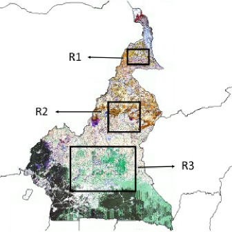
To illustrate our analytical results and highlight important ecological parameters, we will perform some numerical simulations. In fact, from the ecological point of view, parameters can change drastically according to the environmental features. For instance, in Cameroon, three different zones can be particularly highlighted. The first zone is Region 1 (R1) where the biomass production is low (the Mean Annual Precipitations (MAP) is less than $650$ mm by year). The second zone is Region 2 (R2) ($650$-$1100$ mm/yr). It has more biomass production by year. The last zone (R3) ($1100-1800$ mm by year) where savannas are observed in some cases in the immediate vicinity of forests (Favier et al. 2012 [44]). Model (1) has 11 parameters. Eight of them $(\gamma_{G},K_{G},\delta_{G0},\alpha,\gamma_{T},K_{T},\delta_{T},\gamma_{TG})$ specify vegetation growth while the others are related to the fire characteristics. Parameter values used are based on literature sources.

Figure 1: Overall vegetation map of Cameroon from Letouzey (1985). The three regions R1, R2 and R3 are indicated by black rectangles.

Table 4: Vegetational Data

	Site name
$\mathbf{Parameters}$	$\mathbf{Semi-arid}$	$\mathbf{Mesic}$	$\mathbf{Humid}$	$\mathbf{Units}$	$\mathbf{Sources}$
	$\mathbf{R1}$	$\mathbf{R2}$	$\mathbf{R3}$
$K_{G}$	$2-5$	$8-10$	$10-20$	t.ha-1	[45, 15]
$\gamma_{G}$	$0.4^{(*)}-1.5^{(**)}$	$1.5-3$	$3-4.6^{(***)}$	yr-1	(∗), (∗∗) [46], (∗∗∗) [13]
$\delta_{G0}$	$0$	$0$	$0-0.9$(4∗)	yr-1	(4∗) [47]
$\lambda_{fG}$	$0.1-0.9$	$0.1-0.9$	$0.1-0.9$	-	assumed, see also [15]
$\alpha$	$2$	$2$	$2$	t.ha-1	Assumed
$\theta$	$2$	$2$	$2$	t.ha-1	Assumed
$K_{T}$	$10-25$	$25-60$	$60-115$	t.ha-1	[48]
$\gamma_{T}$	$0.3^{(a)}-0.9$	$0.9-1.2$	$1.2-7.2^{(b)}$	yr-1	(a) [46], (b) [49]
$\delta_{T}$	$0$	$0$	$0-0.015^{(5*)}$	yr-1	(5∗) [5]
$\lambda_{fT}$	$0.1-0.5$	$0.1-0.5$	$0.1-0.4$	-	Assumed
$\tau$	$\geq 10$	$2-8$	$0.5-2$	yr	Overall expert-based knowledge,
					in addition to [13, 44]
$\gamma_{TG}$	$(-0.01)-0.03$	$0.01-0.08$	$0.03-0.09$	ha.t-1.yr-1	[10], [15]
					(after reinterpretation)

Note 5.1

Range values for parameters ($K_{G}$, $k_{T}$, $\lambda_{fG}$, $\lambda_{fT}$, $\tau$, $\gamma_{TG}$) used for the simulation runs. Early fire destroy only $25\%$ (Abbadie et al., 2006 [15]) of grass biomass, while late fires can destroy up to $90\%$ of biomass.

Our numerical analysis focuses on Cameroon as part of Central Africa where we find a summary of African natural conditions, from humid equatorial climate near the Atlantic Ocean, up to the arid Sahelian tropical climate in the region of Lake Chad.

The first site is R1. It corresponds to semi-arid zones. Grasses may be dominant while trees are generally of low stature. Trees are resource-limited, and the resource competition with grasses and between trees are the key factor determining savanna existence (Baudena et al., 2014 [50]; Tchuinte et al., 2014 [30]). In Cameroon, R1 (small black rectangle in Figure 1) corresponds to the dry tropical climate of the extreme North Country, from Ka l in Maroua and Mora, and from Yagoua to Kouss ri, Makary and Lake Chad. At the edges of Lake Chad, there is only 3 months of rain with $500$ mm/yr.

The second region, R2, represents a mesic zone. Here the MAP varies from $650$ mm/yr to $1100$ mm/yr. In Cameroon it is located at the Northern part, from Adamawa to the Mandara Mountains (see the middle black rectangle in fig 1). There are two seasons covering the whole of Adamawa plateau, from Banyo to Ngaroundere and Meiganga. It has been argued, that mesic savannas are unstable compared to forest and disturbance-dependent with respect to fires (Sankaran et al., 2005 [24]), which prevent tree invasion, because they occur regularly during the dry season. Grasses benefit from fire because they recover faster than trees after fires, and profit of open spaces to growth. Thus grass-fire feedback is a characteristic feature that leads to savanna or grassland persistence.

High rainfall occurring in wet African savannas directly reduce the role of water as limiting factor. The last region (R3) that we are interested in corresponds to humid areas where MAP varies between $1100$ mm/yr and $1800$ mm/yr. In this region, the high water resource available enables high fuel (grass biomass) production and therefore fires are more frequent and of greater impact on seedlings. The grass-fire feedback in R3 leads to a bistability of savanna and forest, as shown using a simple continuous models (e.g. Tchuinte et al., 2014 [30]; Staver and Levin, 2012 [51]) and evidenced from remote sensing data by Favier et al. (2012) [44]. In Cameroon, R3 (see the big black rectangle in Figure 1) encompasses two sub-zones: a sub-zone of transition between equatorial and tropical climates, and a sub-zone which corresponds to the equatorial climate itself. Concerning the first one, the MAP is between $1100$ mm/yr and $1500$ mm/yr. It is observed from Bafia to Bertoua, Batouri and from Yoko to Betare Oya, Garoua Boula . The second sub-zone is a site covering the entire South of the Country from Yaounde (1564 mm/yr) to Yokadouma, from Ebolowa to Ambam, Mouloundou and Ouesso (Congo). It extented near the Gabonese borber (1700mm). In both the two sub-zones there are four distinct seasons (two dry seasons alternating with two wet seasons with unequal intensity). At the South Cameroon near the Gabonese border (11 months of rainy season), there is a close canopy forest (see fig 1). Above R3 (at the highest end of the rainfall range which is $2000$ mm/yr), fires are totally suppressed and only forests are observed, since grass growth is inhibited by tree shade.

In the next section we present some numerical simulations. The fundamental tasks in studying disturbance are to discriminate between fluctuations that are extraordinary and those that are usual (McNaughton 1992 [52]). In our simulations, we assume that the ecological system is not impacted by Human and Animals (grazing and browsing), i.e. $\delta_{G0}=\delta_{T}=0$.

5.2 Simulations to illustrate bifurcations due to $\gamma_{TG}$ in regions R1, R2, and R3

5.2.1 Simulations in region R1

According to table 4, we choose the following values of parameters for region R1:

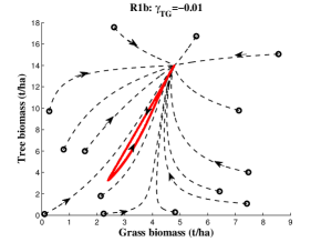
Table 5: Parameters values related to figure 2

$K_{G}$	$\gamma_{G}$	$\delta_{G0}$	$K_{T}$	$\gamma_{T}$	$\delta_{T}$	$\alpha$	$\tau$	$\lambda_{fT}$	$\lambda_{fG}$
$4$	$0.7$	$0$	$14$	$0.75$	$0$	$2$	$12$	$0.9$	$0.5$

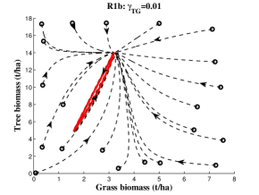
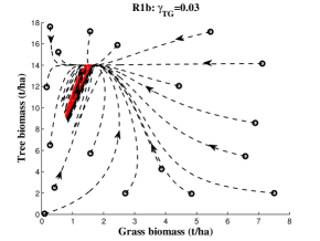
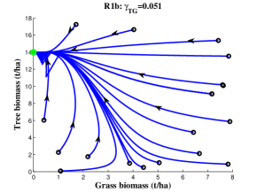
Taking $\gamma_{TG}=[-0.01,0.01,0.03,0.051]$, and, using Table 3, we obtain Table 6. Figure 2 illustrates also the expected behaviours.

Table 6: Thresholds Table related to Table 5 and Figure 2

Panel	$\mathcal{R}_{01}$	$\mathcal{R}_{0,pulse}^{\tilde{G}_{e}}$	$\tilde{\mathcal{R}}_{0,\mathcal{R}_{01}}$	$\mathcal{R}_{0,pulse}^{*}$	$\mathcal{R}_{0,stable}^{*}$	$\mathcal{R}_{0,stable}^{**}$	Case
a	$-$	$>1$	$>1$	$>1$	$>1$	$>1$	XIII
b,c	$>1$	$>1$	$>1$	$>1$	$>1$	$>1$	XIII
d	$<1$	$>1$	$-$	$>1$	-	-	V

Figure 2: Phase diagrams in R1. Panels $\mathbf{a}$ and $\mathbf{b}$ ($\mathbf{c}$ and $\mathbf{d}$) show the impact of the tree/grass competition parameter (see panels panel $\mathbf{c}$ and $\mathbf{d}$). When $\gamma_{TG}$ increases and exceeds a critical value, the attracting state of the system shifts from periodic savanna to a forest equilibrium (in fact, dense thickets).

In semi-arid areas, Tree-Grass interactions are predominantly influenced by competition for soil water (e.g. Walker et al. 1981 [53]). However, shading by tree foliage under arid climate can also increase grass production under the tree crown (Abbadie et al. 2006 [15]) and more generally can increase the water budget below the canopy (Barbier et al. 2008 [54]). Hence the influence of trees on grasses can range from facilitation to competition. Figure 2 shows the influence of tree/grass interactions in R1. For higher values of $\gamma_{TG}$, trajectories converge to the forest equilibrium (see panel $\mathbf{d}$) corresponding, in fact to dense thickets. When $\gamma_{TG}$ is small, and even negative (positive effect on the grass biomass), the system converges to a periodic Tree-Grass coexistence equilibrium with fairly large amplitudes in the tree biomass (compare panels $\mathbf{a}$ and $\mathbf{b}$), or with small grass biomass (see panel $\mathbf{c}$). Here $\gamma_{TG}$ is an influential parameter since it permits a transition from savanna to forest. This result joins those of Sankaran et al. (2005) [24] which argued that in R1, savannas are stable in the sense that tree biomass and cover are primarily limited by resources (see panels $\mathbf{a}$ and $\mathbf{c}$ in Figure 2). Therefore, the competition parameter $\gamma_{TG}$ is an important driver of Tree-Grass dynamics in R1 where fires return time are typically higher than 10 years and therefore are not necessary for grass-tree coexistence. Our Tree-Grass impulsional model shows that in R1, there is only a stable periodic grass-tree equilibrium or a stable forest equilibrium (see panels $\mathbf{a}$ and $\mathbf{d}$ in Figure 2).

5.2.2 Simulations in region R2

Let us consider the following values of parameters according to table 4.

Table 7: Parameters values related to figure 3

$K_{G}$	$\gamma_{G}$	$\delta_{G0}$	$K_{T}$	$\gamma_{T}$	$\delta_{T}$	$\alpha$	$\tau$	$\lambda_{fT}$	$\lambda_{fG}$
$8$	$1.9$	$0$	$30$	$0.9$	$0$	$2$	$5$	$0.5$	$0.6$

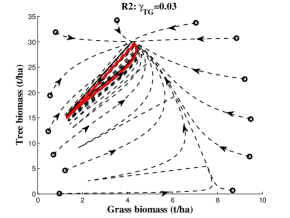
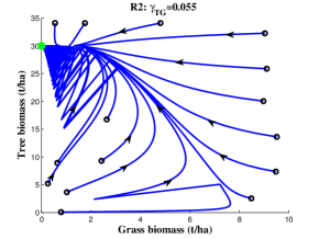
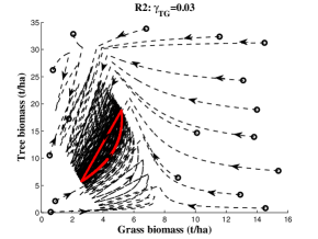
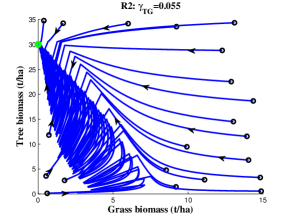
According to Table 3 and Table 7, with $\gamma_{TG}=[0.01,0.02,0.03,0.055]$, we derive, in Table 8, the behaviours of the Tree-Grass system. See also Figure 3, page 3.

Table 8: Thresholds Table related to Table 7 and Figure 3

Panel	$\mathcal{R}_{01}$	$\mathcal{R}_{0,pulse}^{\tilde{G}_{e}}$	$\tilde{\mathcal{R}}_{0,\mathcal{R}_{01}}$	$\mathcal{R}_{0,pulse}^{*}$	$\mathcal{R}_{0,stable}^{*}$	$\mathcal{R}_{0,stable}^{**}$	Case
a,b,c	$>1$	$>1$	$>1$	$>1$	$>1$	$>1$	XIII
d	$>1$	$>1$	$<1$	$>1$	$-$	$-$	X

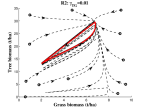
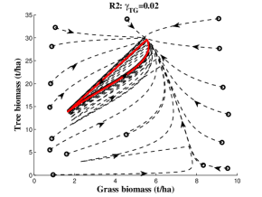
Figure 3 below illustrates the bifurcation due to the competition parameter in Region (R2). The forest equilibrium is stable for $\gamma_{TG}=0.055$ a value in the upper range of plausible values (see panel $\mathbf{d}$). When $\gamma_{TG}$ decreases, the system converges to a savanna periodic equilibrium (see panel $\mathbf{a,b,c}$). We note also that $\gamma_{TG}$ has an impact on the amplitude of the periodic savanna equilibrium and the maximal amount of grass biomass.

Figure 3: Phase diagrams in R2 with a period of fire of $\tau=5$ years.

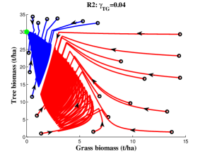
Increasing the impact of fire on trees via an increase of the "$\lambda_{fT}$" coefficient, a bistability between forest and savanna occurs in R2 (see figure 4 below).

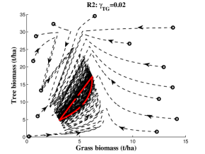
Table 9: Parameters values related to figure 4

$K_{G}$	$\gamma_{G}$	$\delta_{G0}$	$K_{T}$	$\gamma_{T}$	$\delta_{T}$	$\alpha$	$\tau$	$\lambda_{fT}$	$\lambda_{fG}$
$8$	$1.5$	$0$	$30$	$0.9$	$0$	$2$	$2.2$	$0.8$	$0.5$

Using the same values for $\gamma_{TG}$, we derive Table 10 and Figure 4.

Table 10: Thresholds Table related to Table 9 and Figure 4

Panel	$\mathcal{R}_{01}$	$\mathcal{R}_{0,pulse}^{\tilde{G}_{e}}$	$\tilde{\mathcal{R}}_{0,\mathcal{R}_{01}}$	$\mathcal{R}_{0,pulse}^{*}$	$\mathcal{R}_{0,stable}^{*}$	$\mathcal{R}_{0,stable}^{**}$	Case
a, b	$>1$	$>1$	$>1$	$>1$	$>1$	$>1$	XIII
c	$>1$	$>1$	$<1$	$>1$	$>1$	$>1$	VIII
d	$<1$	$>1$	$-$	$>1$	$-$	$-$	V

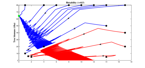
Figure 4: Phase diagrams in R2 with a period of fire of $\tau=5$ years (Table 9) and a stronger impact of fire than in Figure 3 via $\lambda_{fT}=0.8$. Panels $\mathbf{a}$, $\mathbf{b}$, $\mathbf{c}$ and $\mathbf{d}$ show the impact of the tree/grass competition parameter.

Figure 4 shows interesting behaviours. In particular, in panel $\mathbf{c}$, we obtain a bistable situation, where the system can either converge to the forest equilibrium or the periodic Tree-Grass equilibrium, depending on the initial values. In that case, we don’t have analytic results that allow us to know what are the basins of attraction of each equilibrium. That is why the use of a well fitted numerical scheme is of utmost importance, in order to capture this essential information. We will show other examples of bistability in the next section.

5.2.3 Simulations in region R3

According to table 4, we first consider the following values for simulations in region R3:

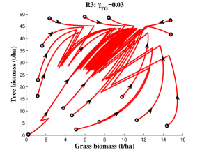
Table 11: Parameters values related to figure 5

$K_{G}$	$\gamma_{G}$	$\delta_{G0}$	$K_{T}$	$\gamma_{T}$	$\delta_{T}$	$\alpha$	$\tau$	$\lambda_{fT}$	$\lambda_{fG}$
$17$	$4.5$	$0$	$45$	$6$	$0$	$2$	$0.6$	$0.4$	$0.4$

Using Table 15 with $\gamma_{TG}=[0.03,0.05,0.07,0.09]$ leads to Table 12 and figure )5.

Table 12: Thresholds Table related to Table 15 and Figure 5

Panel	$\mathcal{R}_{01}$	$\mathcal{R}_{0,pulse}^{\tilde{G}_{e}}$	$\tilde{\mathcal{R}}_{0,\mathcal{R}_{01}}$	$\mathcal{R}_{0,pulse}^{*}$	$\mathcal{R}_{0,stable}^{*}$	$\mathcal{R}_{0,stable}^{**}$	Case
a,b,c	$>1$	$>1$	$>1$	$>1$	$>1$	$>1$	XIII
d	$>1$	$>1$	$<1$	$>1$	$-$	$-$	X

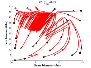
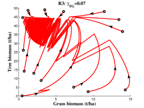
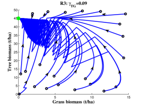
Figure 5: Phase diagrams in R3. This figure shows two equilibria: forest and periodic savanna.

In the humid zone, the vegetation is intrinsically dominated by trees which exert competitive pressure on grasses, such that grasses are suppressed or even out-competed (Scholes and Walker 1993 [34], see panel d). Figure 5 illustrates the effect of the competition parameter in R3.

Note 5.2

Using realistic ranges for parameters, we show that in R3, a stable periodic savanna equilibrium may appear but also a stable forest equilibrium, for sufficiently high values of $\gamma_{TG}$. However we cannot have a periodic grassland equilibrium. In R2, it is possible to have forest equilibrium and periodic savanna.

Like in Region R2, bistable situations can occur in region R3. Let us first consider the following parameter values

Table 13: Parameters values related to figure 6

$K_{G}$	$\gamma_{G}$	$\delta_{G0}$	$\lambda_{fG}$	$K_{T}$	$\gamma_{T}$	$\delta_{T}$	$\lambda_{fT}$	$\tau$	$\alpha$	$\gamma_{TG}$
$19$	$3.1$	$0.1$	$0.5$	$50$	$1.5$	$0.015$	$0.6$	$0.5$	$2$	$0.09$

Table 14: Threshold values related to figure 6

$\mathcal{R}_{01}$	$\mathcal{R}_{0,pulse}^{\tilde{G}_{e}}$	$\tilde{\mathcal{R}}_{0,\mathcal{R}_{01}}$	$\mathcal{R}_{0,pulse}^{*}$	$\mathcal{R}_{0,stable}^{*}$	$\mathcal{R}_{0,stable}^{**}$	Case
$<1$	$>1$	$-$	$<1$	$-$	$-$	II

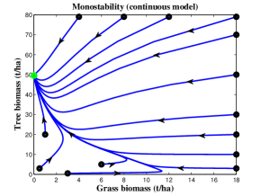
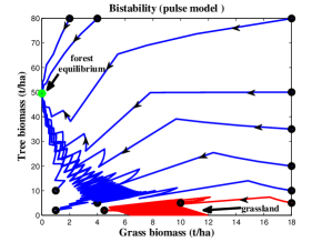
The mathematical analysis shows that there is a bistability between the forest equilibrium and a periodic grassland equilibrium (see line $\mathbf{II}$ in table 3). Panel $\mathbf{a}$ (pulse model) in figure 6 illustrates two basins of attraction: one in favour of forest equilibrium; another in favour of the periodic grassland equilibrium (bistability as in line $\mathbf{II}$ in table 3). For the same values of parameters, the continuous model does not yield bistability (see panel $\mathbf{b}$ in 6): the only equilibrium is the forest equilibrium [30].

Figure 6: Comparison of the pulse vs. continuous models in reference to R3. The continuous model presents a forest equilibrium which is GAS (see panel $\mathbf{b}$). In contrast, the discrete model shows two equilibria: the forest (as for the continuous model) and the periodic grassland (see panel $\mathbf{a}$). Depending of the initial conditions the system converges to a stable periodic grassland or to a stable forest equilibrium.

We have shown that the interspecific parameter, $\gamma_{TG}$ plays a great role in the dynamics. However, fire period can also have an impact on the dynamics of the Tree-Grass system in R3 as in the two previous zones. Let us consider the following parameter values:

Table 15: Parameters values related to figure 7

$K_{G}$	$\gamma_{G}$	$\delta_{G0}$	$\lambda_{fG}$	$K_{T}$	$\gamma_{T}$	$\delta_{T}$	$\lambda_{fT}$	$\alpha$	$\gamma_{TG}$
$19$	$3.1$	$0.1$	$0.5$	$65$	$1.5$	$0.015$	$0.6$	$2$	$0.04$

According to Tables 3 and 15, we derive, in Table 16, the different possible dynamics ot the Tree-Grass system:

Table 16: Threshold values related to figure 7

Panel	$\mathcal{R}_{01}$	$\mathcal{R}_{0,pulse}^{\tilde{G}_{e}}$	$\tilde{\mathcal{R}}_{0,\mathcal{R}_{01}}$	$\mathcal{R}_{0,pulse}^{*}$	$\mathcal{R}_{0,stable}^{*}$	$\mathcal{R}_{0,stable}^{**}$	Case
a	$>1$	$>1$	$<1$	$<1$	$-$	$-$	VII
b	$>1$	$>1$	$<1$	$>1$	$>1$	$>1$	VIII

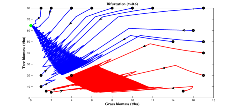
It has been evidenced that in humid savannas, fire is necessary to establish the Tree-Grass coexistence equilibrium (Sankaran et al. 2005 [24]). However, various bistabilities occur: between forest and grassland (see panel $\mathbf{a}$ in figure 7); between forest and savanna (see panel $\mathbf{b}$ in figure 7). The system can shift from $\mathbf{a}$ to $\mathbf{b}$ (bifurcation) when the fire period increases. When $\tau=0.5$ (two fires a year in a sub-equatorial context), we have a bistability case: with a forest equilibrium and a periodic grassland equilibrium (see panel $\mathbf{a}$ in figure 7 which illustrates case $\mathbf{VII}$ in table 3). When the fire period increases by $10\%$ i.e. $\tau=0.6$, there is still bistability case, but the periodic grassland equilibrium is replaced by a periodic savanna equilibrium. This corresponds to line $\mathbf{VIII}$ in table 3 and to panel $\mathbf{b}$ in figure 7.

Figure 7: Fire mediated Tree-Grass mixtures and changes in their physiognomies according to the fire period. Panel $\mathbf{a}$ shows two bistable equilibria (a forest equilibrium and a periodic grassland equilibrium (see $\mathbf{VII}$ in table 3)). From $\tau=0.5$ to $0.6$, the ecosystem changes. Panel $\mathbf{b}$ illustrates two bistable equilibria (the periodic savanna and the forest equilibrium (see $\mathbf{VIII}$ in table 3)).

In R3, both forest-grassland, and forest-savanna equilibria are predicted (see panels $\mathbf{a}$ and $\mathbf{b}$ in Figure 7). The fire period is a bifurcation parameter that shapes the Tree-Grass dynamics in R3.

6 Conclusion

Savannas are complex systems due to the interaction of trees and grasses which are frequently mediated by disturbances and notably by fires. The broad objective of this work was to develop a predictive understanding of Tree-Grass dynamics across rainfall gradients in Africa on the basis of a minimalistic model. This is done using specific features of three ecological contexts: semi-arid, mesic and humid. They represent different ecological conditions in terms of rainfall amount and deriving variations of most of the parameters used in the model. We formalize a new model of Tree-Grass interactions. The novelty of the model, with respect to other models (Staver et al., 2011 [28], Accatino et al., 2010 [26], [30]) is that fire is considered as discrete events with high or low return times. In addition, fire frequencies and fire intensities are decoupled. Discrete events are typically modelled by impulsive differential equations. We show here that this framework yields richer qualitative behaviours than continuous modelling (see figure 6). Several authors, in order to deal with the stochastic occurrence of fire have modelled fire through purely stochastic differential equations (D’Odoricco et al. 2006 [25], Beckage et al. 2011 [27], De Michele and Accatino 2014 [55]). However results of those stochastic models are often obtained numerically by iterating the equations given parameter values and initial conditions and the authors have difficulties to verify mathematically that the qualitative properties (e.g existence of equilibria and their stability) of the model are preserved in their simulations. By contrast, at least qualitatively, our impulsive model is lend itself to a comprehensive qualitative analysis of the possible dynamic outcomes and properties of the system. For this raison, it is perhaps interesting to used impulsive framework to look at least qualitatively at the problem of predictability of discrete fire impacts in tropical savannas. The impulsive modelling of fire suggests ways for deriving from a minimal continuous fire model (e.g. Tchuinte et al., 2014 [30]) more realistic discrete fire model. The theory of IDE allows for more detailed analyses of the system than stochastic differential equations. Further, using IDE technique, we can highlight mathematically thresholds that summarize the Tree-Grass interaction (see table 3) and point out bifurcation parameters.

The impulsive model illustrates different kinds of dynamics which can be observed across of rainfall gradients in Africa. The model generates savanna equilibria in all the three regions. It means that trees are able to persist while not reaching $80$-$100\%$ cover all over the wide range of rainfall considered. However, at high rainfall sites such like the boundaries of the tropical rainforests of central Africa, the vegetation is due to be dominated by trees and may even reach a closed tree cover in the absence of recurrent fires of low return times which are fostered by high grass production. On the other hand, trees can reach high individual biomass and exert intense light competition on grasses, such that grasses are suppressed or even out-competed (Scholes and Walker 1993 [34]). This explains why forest may be stable in R3 and even in R2. However, tree cover can also facilitate the growth of grasses, i.e. $\gamma_{TG}<0$ in arid conditions (i.e. R1) by limiting soil water losses from transpiration in the topsoil. In R1, we show that the existence of savanna is mainly due to the competition parameter. Thus, only two equilibria are possible: a forest equilibrium and a periodic savanna equilibrium. The bifurcation from the forest to the periodic savanna is related to the resource competition parameter, $\gamma_{TG}$. This result joins those of Sankaran et al., (2005) [24] that argued that in drier sites, savannas are stable in the sense that tree cover is intrinsically limited by resource (and this contributes to the low value of KT) and fire is not necessary for Tree-Grass coexistence. Recent modelling studies by Baudena et al. (2014) [50] confirm that in semi-arid savannas, while trees are water-limited, the water competition with grasses is also a key factor determining savanna existence.

We show that in all regions, the competition parameter plays a great role: it is a bifurcation parameter whatever the context.

Grass-fire feedback principally occurs in mesic and humid areas. No savanna or grassland would emerge without this positive feedback in Regions R2 and R3. Using realistic parameter values, we show that in R2 (mesic area) forest and savanna are more present than grassland. In R3, in humid area, two bistability situations may occur: bistability between forest and grassland and bistability between forest and (periodic) savanna. In the equatorial climate in Southern Cameroon (Central Africa), there is forest-savanna contact in three sites inside R3: Akonolinga, Bertoua and Mbam-Kim (Youta 1998 [56]). Bistability of forest and grassland can be found in the equatorial and tropical climate of transitions ($1100$-$1500$ mm/yr) where fires are usually occurring every $1$-$5$ years (Frost and Robertson, 1987 [11], Favier et al. 2012 [44]). In this area and due to the large grass biomass, flame height is usually $2$-$3$ m high (Frost and Robertson, 1987 [11]). Therefore, a severe fire could have a great impact on young trees/shrubs. In R3, water availability enables high fuel production. As a result, fire is severe and may occur as frequently as $0.5$-$1$ yr. Thus, fire has a stabilizing role of grassland and savannas by preventing tree invasion on long time scales, freezing the forest-savanna boundary in a historical position (Gillon, 1983 [14]). We show from our model that in R3 the Tree-Grass system can shift from bistability between forest and grassland to bistability between forest and savanna due to fire period.

To conclude: (i) in all regions Tree-Grass competition is the most important parameter for Tree-Grass co-existence; (ii) in R2 and R3, fire period can also be a bifurcation parameter. Thus, the fire period (and fire intensities) and the competition parameters are the main determinant in the Tree-Grass dynamics; (iii) Modelling fire as pulse events provides more realistic situations than modelling fire as continuous events.

APPENDICES

Some detail of the proofs of results associated with system (1) are provided.

Appendix A: Proof of Lemma 3.1

It is obvious that $G=0$, and $T=0$ are vertical and horizontal null-clines respectively. Then, no trajectory can cut these axes. Thus, the positive cone $\mathbf{R}_{+}^{2}$ is positively invariant for $(\ref{Impuleq1})$ because, all trajectories that start in $\mathbf{R}^{2}_{+}$ remain in $\mathbf{R}^{2}_{+}$ for all positive time. From system $(\ref{Impuleq1})$, with the initial conditions $T(t_{0})=T_{0}>0$ and $G(t_{0})=G_{0}>0$, we obtain the following system

$$\left\{\begin{array}[]{lcl}\displaystyle\frac{dG}{dt}\leq(\gamma_{G}-\delta_{G0})G-\mu_{G}G^{2},\\ \\ \displaystyle\frac{dT}{dt}\leq(\gamma_{T}-\delta_{T})T-\mu_{T}T^{2},\\ \\ T(t_{0})=T_{0},\\ \\ G(t_{0})=G_{0}.\end{array}\right.$$ (12)

Using the maximum principle, we deduce that

$$\left\{\begin{array}[]{lcl}G\leq\displaystyle\frac{G_{0}}{\displaystyle\frac{G_{0}}{X_{G}}+\left(1-\displaystyle\frac{G_{0}}{X_{G}}\right)\exp\left\{-X_{G}\mu_{G}t\right\}},\\ \\ T\leq\displaystyle\frac{T_{0}}{\displaystyle\frac{T_{0}}{Y_{T}}+\left(1-\displaystyle\frac{T_{0}}{Y_{T}}\right)\exp\left\{-Y_{T}\mu_{T}t\right\}},\\ \end{array}\right.$$ (13)

When $t\rightarrow\infty$, we obtain

$$\left\{\begin{array}[]{lcl}\lim\limits_{t\rightarrow\infty}G(t)\leq X_{G}=\displaystyle\frac{\gamma_{G}-\delta_{G0}}{\mu_{G}}=K_{G}\left(1-\displaystyle\frac{\delta_{G0}}{\gamma_{G}}\right),\\ \\ \lim\limits_{t\rightarrow\infty}T(t)\leq Y_{T}=\displaystyle\frac{\gamma_{T}-\delta_{T}}{\mu_{T}}=K_{T}\left(1-\displaystyle\frac{\delta_{T}}{\gamma_{T}}\right).\\ \end{array}\right.$$ (14)

Hence, when $\gamma_{G}>\delta_{G0}$ and $\gamma_{T}>\delta_{T}$, all trajectories of system $(\ref{Impuleq1})$ that reach the neighbourhood of $\mathcal{B}$ converge inside as $t$ tends to infinity. Since $\mathcal{B}\subseteq\mathbf{R}_{+}^{2}$, then $\mathcal{B}$ is positively invariant and attracting for system $(\ref{Impuleq1})$.

Appendix B: Proof of theorem 3.1 (existence of the semi-trivial periodic equilibrium)

Let $T(t)\equiv 0$, from system (1), we have the following simple logistic impulsive differential system:

$$\left\{\begin{array}[]{lcl}\displaystyle\frac{dG}{dt}&=&r_{G}G-\mu_{G}G^{2},\hskip 14.22636ptt\neq t_{n},\\ \\ G(t_{n}^{+})&=&G(t_{n})-\lambda_{fG}G(t_{n})\hskip 14.22636ptt=t_{n}.\end{array}\right.$$ (15)

The solution of system (15) is given in [57]. Here, is shown in detail the proof.

Setting $X=\displaystyle\frac{1}{G}$ in the first equation of system $(\ref{Impuleq19})$, we have the following differential equation

$$\frac{dX}{dt}=-r_{G}X+\mu_{G}.$$

Integrating

$$\frac{dX}{dt}=-r_{G}X$$

from $n\tau$ to $t$, we obtain

$$X(t)=ae^{-r_{G}(t-n\tau)},\hskip 14.22636pta\in\mathbf{R}.$$ (16)

Using the variation of the constant $a$, we have the following differential equation

$$\frac{da}{dt}=\mu_{G}e^{r_{G}(t-n\tau)}.$$

Thus, we have

$$a(t)=\displaystyle\frac{1}{X_{G}}e^{r_{G}(t-n\tau)}+b,\hskip 14.22636ptb\in\mathbf{R}.$$ (17)

Substituting $(\ref{Impuleq21})$ in $(\ref{Impuleq20})$, we obtain

$$X(t)=\displaystyle\frac{1}{X_{G}}+be^{-r_{G}(t-n\tau)},\hskip 14.22636ptb\in\mathbf{R}.$$ (18)

Considering $X(t)=\displaystyle\frac{1}{G(t)}$ in $(\ref{Impuleq22})$, we have

$$\frac{1}{G(t)}=\displaystyle\frac{1}{X_{G}}+be^{-r_{G}(t-n\tau)},\hskip 14.22636ptb\in\mathbf{R},$$

this implies that,

$$G(t)=\displaystyle\frac{1}{\displaystyle\frac{1}{X_{G}}+be^{-r_{G}(t-n\tau)}},\hskip 14.22636ptb\in\mathbf{R}.$$ (19)

At $t=n\tau$, we have

$$G(n\tau)=\displaystyle\frac{1}{\displaystyle\frac{1}{X_{G}}+b},\hskip 14.22636ptb\in\mathbf{R},$$

and therefore

$$b=\displaystyle\frac{1}{G(n\tau)}-\displaystyle\frac{1}{X_{G}}.$$

Substituting the expression of $b$ in $(\ref{Impuleq23})$, we obtain

$$G(t)=\displaystyle\frac{G(n\tau)e^{r_{G}(t-n\tau)}}{1+\displaystyle\frac{G(n\tau)}{X_{G}}\left(e^{r_{G}(t-n\tau)}-1\right)}.$$ (20)

We have

$$G(t_{n+1}^{+})=G((n+1)\tau)=\displaystyle\frac{G(n\tau)e^{r_{G}\tau}}{1+\displaystyle\frac{G(n\tau)}{X_{G}}\left(e^{r_{G}\tau}-1\right)}.$$ (21)

By substituting $(\ref{Impuleq25})$ into the second equation of $(\ref{Impuleq19})$, we obtain

$$G(n\tau)=(1-\lambda_{fG})G((n+1)\tau)=\displaystyle\frac{(1-\lambda_{fG})G(n\tau)e^{r_{G}\tau}}{1+\displaystyle\frac{G(n\tau)}{X_{G}}\left(e^{r_{G}\tau}-1\right)},$$

which implies that

$$G(n\tau)=\displaystyle\frac{X_{G}\{(1-\lambda_{fG})e^{r_{G}\tau}-1\}}{e^{r_{G}\tau}-1}.$$ (22)

Substituting the expression of $G(n\tau)$ into $(\ref{Impuleq24})$, we have

$$G(t) =\displaystyle\frac{X_{G}\{(1-\lambda_{fG})e^{r_{G}\tau}-1\}e^{r_{G}(t-n\tau)}}{(e^{r_{G}\tau}-1)\left\{1+\displaystyle\frac{\{(1-\lambda_{fG})e^{r_{G}\tau}-1\}(e^{r_{G}(t-n\tau)}-1)}{(e^{r_{G}\tau}-1)}\right\}}$$

$$=\displaystyle\frac{X_{G}\{(1-\lambda_{fG})e^{r_{G}\tau}-1\}e^{r_{G}(t-n\tau)}}{(e^{r_{G}\tau}-1)+\{(1-\lambda_{fG})e^{r_{G}\tau}-1\}(e^{r_{G}(t-n\tau)}-1)}$$

$$=\displaystyle\frac{X_{G}\{(1-\lambda_{fG})e^{r_{G}\tau}-1\}e^{r_{G}(t-n\tau)}}{\{(1-\lambda_{fG})e^{r_{G}\tau}-1\}e^{r_{G}(t-n\tau)}+\lambda_{fG}e^{r_{G}\tau}}.$$

Thus, when $\mathcal{R}_{0,pulse}^{\tilde{G}_{e}}>1$, there exists

$$\tilde{G}_{e}(t)=X_{G}\displaystyle\frac{\{(1-\lambda_{fG})e^{r_{G}\tau}-1\}e^{r_{G}(t-n\tau)}}{\{(1-\lambda_{fG})e^{r_{G}\tau}-1\}e^{r_{G}(t-n\tau)}+\lambda_{fG}e^{r_{G}\tau}}>0,\hskip 14.22636ptt\in[n\tau,(n+1)\tau[,n=0,1,2,....$$ (23)

This completes the proof.

Appendix C: Proof of theorem 3.2.

We calculate the unique periodic equilibrium.
Set $X=\displaystyle\frac{1}{T}$ in the second equation of $(\ref{Impuleq1})$. We obtain the following differential equation

$$\begin{array}[]{lcl}\displaystyle\frac{dX}{dt}=-r_{T}X+\mu_{T}.\end{array}$$ (24)

Integrate system (24) in $n\tau\leq t<(n+1)\tau$, we have

$$\begin{array}[]{lcl}T(t)&=&\displaystyle\frac{T(n\tau)e^{r_{T}(t-n\tau)}}{1+\displaystyle\frac{T(n\tau)}{Y_{T}}\left[e^{r_{T}(t-n\tau)}-1\right]}.\end{array}$$ (25)

Now, we solve the first equation of $(\ref{Impuleq1})$

$$\begin{array}[]{lcl}\displaystyle\frac{dG}{dt}=(\gamma_{G}-\delta_{G0})G-\mu_{G}G^{2}-\gamma_{TG}TG,\end{array}$$ (26)

where the expression of $T$ is given by $(\ref{Impuleq50})$.

Set $Y=\displaystyle\frac{1}{G}$ in $(\ref{Impuleq51})$. We have the following differential equation

$$\begin{array}[]{lcl}\displaystyle\frac{dY}{dt}&=&-(r_{G}-\gamma_{TG}T(t))Y+\mu_{G}.\end{array}$$ (27)

Integrating

$$\begin{array}[]{lcl}\displaystyle\frac{dY}{dt}&=&-(r_{G}-\gamma_{TG}T(t))Y,\end{array}$$ (28)

from $n\tau$ to $t$, we have

$$\ln(Y) =-r_{G}(t-n\tau)+\gamma_{TG}\int_{n\tau}^{t}T(u)du+a,~{}~{}a\in\mathbf{R}$$

$$=-r_{G}(t-n\tau)+\displaystyle\frac{\gamma_{TG}}{\mu_{T}}\ln\left[1+\displaystyle\frac{T(n\tau)}{Y_{T}}\left[e^{r_{T}(t-n\tau)}-1\right]\right]+a,~{}~{}a\in\mathbf{R},$$

which implies that,

$$\begin{array}[]{lcl}Y(t)&=&Pe^{-m(t,n\tau,T(n\tau))},~{}~{}P\in\mathbf{R},\end{array}$$ (29)

where,

$$\begin{array}[]{lcl}m(t,n\tau,T(n\tau))&=&r_{G}(t-n\tau)+\displaystyle\frac{\gamma_{TG}}{\mu_{T}}\ln\left[\displaystyle\frac{1}{1+\displaystyle\frac{T(n\tau)}{Y_{T}}\left[e^{r_{T}(t-n\tau)}-1\right]}\right].\end{array}$$ (30)

Variation of $P$ gives

$$\begin{array}[]{lcl}P(t)=\mu_{G}\int_{n\tau}^{t}\chi(u,n\tau,T(n\tau))du+b,~{}~{}b\in\mathbf{R}\end{array}$$ (31)

where,

$$\begin{array}[]{lcl}\chi(t,n\tau,T(n\tau))=e^{m(t,n\tau,T(n\tau))}.\end{array}$$ (32)

Then, we have

$$Y(t)=\displaystyle\frac{P(t)}{\chi(t,n\tau,T(n\tau))},$$

which implies that

$$\begin{array}[]{lcl}G(t)&=&\displaystyle\frac{G(n\tau)\chi(t,n\tau,T(n\tau))}{1+\mu_{G}G(n\tau)\int_{n\tau}^{t}\chi(u,n\tau,T(n\tau))du}.\end{array}$$ (33)

From $(\ref{Impuleq50})$ and $(\ref{Impuleq58})$, we have

$$\left\{\begin{array}[]{lcl}G(t)&=&\displaystyle\frac{G(n\tau)\chi(t,n\tau,T(n\tau))}{1+\mu_{G}G(n\tau)\int_{n\tau}^{t}\chi(u,n\tau,T(n\tau))du},\\ \\ T(t)&=&\displaystyle\frac{T(n\tau)e^{r_{T}(t-n\tau)}}{1+\displaystyle\frac{T(n\tau)}{Y_{T}}(e^{r_{T}(t-n\tau)}-1)},\end{array}\right.$$ (34)

where $G(n\tau)$ and $T(n\tau)$ are values of grasses and trees biomasses respectively, immediately after the $n^{th}$ pulse of fire at the time $n\tau$. $G(n\tau)$ and $T(n\tau)$ can be viewed as the initial values of $(\ref{Impuleq1})$ in the interval $[n\tau,(n+1)\tau[$. The initial values may change in different intervals. For all $t\in[n\tau,(n+1)\tau[$, using the fact that,

$$\left\{\begin{array}[]{lcl}G(t_{n}^{+})=G(t_{n})-\lambda_{fG}G(t_{n}),\\ \\ T(t_{n}^{+})=T(t_{n})-\lambda_{fT}\omega(\lambda_{fG}G(t_{n}))T(t_{n}),\\ \end{array}\right.$$ (35)

we have the following discrete system for $G(n\tau)$ and $T(n\tau)$

$$\left\{\begin{array}[]{lcl}G((n+1)\tau)&=&\displaystyle\frac{(1-\lambda_{fG})G(n\tau)\chi((n+1)\tau,n\tau,T(n\tau))}{1+\mu_{G}G(n\tau)\int_{n\tau}^{(n+1)\tau}\chi(u,n\tau,T(n\tau))du},\\ \\ T((n+1)\tau)&=&\displaystyle\frac{(1-\lambda_{fT}\omega(\lambda_{fG}G(n\tau)))T(n\tau)e^{r_{T}\tau}}{1+\displaystyle\frac{T(n\tau)}{Y_{T}}(e^{r_{T}\tau}-1)}.\\ \end{array}\right.$$ (36)

Setting

$$\left\{\begin{array}[]{lcl}U(G(n\tau),T(n\tau))&=&\displaystyle\frac{(1-\lambda_{fG})G(n\tau)\chi((n+1)\tau,n\tau,T(n\tau))}{1+\mu_{G}G(n\tau)\int_{n\tau}^{(n+1)\tau}\chi(u,n\tau,T(n\tau))du},\\ \\ V(G(n\tau),T(n\tau))&=&\displaystyle\frac{(1-\lambda_{fT}\omega(G(n\tau)))T(n\tau)e^{r_{T}\tau}}{1+\displaystyle\frac{T(n\tau)}{Y_{T}}(e^{r_{T}\tau}-1)},\\ \end{array}\right.$$ (37)

implies that system $(\ref{Impuleq61})$ is equivalent to

$$\left\{\begin{array}[]{lcl}G((n+1)\tau)&=&U(G(n\tau),T(n\tau)),\\ \\ T((n+1)\tau)&=&V(G(n\tau),T(n\tau)).\\ \end{array}\right.$$ (38)

The existence of a periodic solution of $(\ref{Impuleq1})$ (with period $\tau$) is equivalent to an existence of the equilibrium of the discrete system $(\ref{Impuleq63})$. This leads to solve the following system

$$\left\{\begin{array}[]{lcl}U(x,y)&=&x,\\ \\ V(x,y)&=&y.\\ \end{array}\right.$$ (39)

We have

$$U(x,y)=x\Leftrightarrow 1+\mu_{G}x\int_{n\tau}^{(n+1)\tau}\chi(u,n\tau,y)du=(1-\lambda_{fG})\chi((n+1)\tau,n\tau,y),$$

which implies that

$$x=\displaystyle\dfrac{(1-\lambda_{fG})\chi((n+1)\tau,n\tau,y)-1}{\mu_{G}\int_{n\tau}^{(n+1)\tau}\chi(u,n\tau,y)du}:=\phi(y).$$ (40)

On the order hand, we also have

$$V(x,y)=y\Leftrightarrow y=\displaystyle\frac{Y_{T}\{(1-\lambda_{fT}\omega(\lambda_{fG}x))e^{r_{T}\tau}-1\}}{(e^{r_{T}\tau}-1)},$$

which implies that

$$\frac{y}{Y_{T}}(e^{r_{T}\tau}-1)+\lambda_{fT}\omega(\lambda_{fG}x)e^{r_{T}\tau}=(e^{r_{T}\tau}-1).$$ (41)

From (41) and the nonnegativity of the variable $y$ and the function $\omega(\lambda_{fG}x)$ with $x>0$, it follows that $y$ must belong to the interval $D=[0,Y_{T}]$. Substituting $x=\phi(y)$ into the left side of (41) yields an equation for $y$,

$$\frac{y}{Y_{T}}(e^{r_{T}\tau}-1)+\lambda_{fT}\omega(\lambda_{fG}\phi(y))e^{r_{T}\tau}-(e^{r_{T}\tau}-1)=0.$$

Set

$$h(y)=\displaystyle\frac{y}{Y_{T}}(e^{r_{T}\tau}-1)+\lambda_{fT}\omega(\lambda_{fG}\phi(y))e^{r_{T}\tau}-(e^{r_{T}\tau}-1).$$ (42)

It is obvious that $h(y)$ is nonnegative and continuously differentiable with respect to $y$. The algebraic calculation shows that

$$\left\{\begin{array}[]{lcl}h(0)&=&\lambda_{fT}\omega(\lambda_{fG}\phi(0))e^{r_{T}\tau}-(e^{r_{T}\tau}-1),\\ \\ h(Y_{T})&=&\lambda_{fT}\omega(\lambda_{fG}\phi(Y_{T}))e^{r_{T}\tau}.\end{array}\right.$$ (43)

We have

$$\phi(0)=\displaystyle\dfrac{(1-\lambda_{fG})\chi((n+1)\tau,n\tau,0)-1}{\mu_{G}\int_{n\tau}^{(n+1)\tau}\chi(u,n\tau,0)du},$$

where

$$\chi((n+1)\tau,n\tau,0)=e^{r_{G}\tau},\hskip 7.11317pt\mbox{and}$$

$$\int_{n\tau}^{(n+1)\tau}\chi(u,n\tau,0)du=\int_{n\tau}^{(n+1)\tau}e^{r_{G}(u-n\tau)}du=\displaystyle\frac{1}{r_{G}}(e^{r_{G}\tau}-1).$$

Then

$$\phi(0)=X_{G}\displaystyle\frac{(1-\lambda_{fG})e^{r_{G}\tau}-1}{e^{r_{G}\tau}-1}=\tilde{G}_{e}(\tau).$$

Note that

$$\tilde{G}_{e}(\tau)>0\Leftrightarrow\mathcal{R}_{0,pulse}^{\tilde{G}_{e}}>1.$$ (44)

From (43), it is easy to see that

$$h(Y_{T})>0.$$ (45)

We also have

$$h(0)<0 \Leftrightarrow\lambda_{fT}\omega(\lambda_{fG}\phi(0))e^{r_{T}\tau}-e^{r_{T}\tau}-1<0$$

$$\Leftrightarrow 1<e^{r_{T}\tau}(1-\lambda_{fT}\omega(\lambda_{fG}\tilde{G}_{e}(\tau)))$$

$$\Leftrightarrow\displaystyle\frac{1}{1-\lambda_{fT}\omega(\lambda_{fG}\tilde{G}_{e}(\tau))}<e^{r_{T}\tau}$$

$$\Leftrightarrow\ln\left(\displaystyle\frac{1}{1-\lambda_{fT}\omega(\lambda_{fG}\tilde{G}_{e}(\tau))}\right)<r_{T}\tau$$

$$\Leftrightarrow 1<\displaystyle\frac{r_{T}}{\displaystyle\frac{1}{\tau}\ln\left(\displaystyle\frac{1}{1-\lambda_{fT}\omega(\lambda_{fG}\tilde{G}_{e}(\tau))}\right)}$$

$$\Leftrightarrow 1<\mathcal{R}_{0,pulse}^{*}.$$

Then

$$h(0)<0\Leftrightarrow\mathcal{R}_{0,pulse}^{*}>1.$$ (46)

Thus, when (45), and $(\ref{Impuleq71})$ are verified, there exists at least one positive zero of $h(y)=0$ in the interval $D$. To have the uniqueness, we show that $h$ is a highly monotone function.

The derivative of $h(y)$ with respect to $y$ is

$$\frac{dh(y)}{dy}=\displaystyle\frac{1}{Y_{T}}(e^{r_{T}\tau}-1)+\phi^{{}^{\prime}}(y)\lambda_{fT}\lambda_{fG}\omega^{{}^{\prime}}(\lambda_{fG}\phi(y))e^{r_{T}\tau},$$

where

$$\phi^{{}^{\prime}}(y)=\phi_{1}^{{}^{\prime}}(y)-\phi_{2}^{{}^{\prime}}(y),$$

with

$$\phi_{1}^{{}^{\prime}}(y)=\displaystyle\frac{(1-\lambda_{fG})\chi^{{}^{\prime}}((n+1)\tau,n\tau,y)\mu_{G}\int_{n\tau}^{(n+1)\tau}\chi(u,n\tau,y)du}{(\mu_{G}\int_{n\tau}^{(n+1)\tau}\chi(u,n\tau,y)du)^{2}},$$

and

$$\phi_{2}^{{}^{\prime}}(y)=\displaystyle\frac{((1-\lambda_{fG})\chi((n+1)\tau,n\tau,y)-1)\mu_{G}\int_{n\tau}^{(n+1)\tau}\chi^{{}^{\prime}}(u,n\tau,y)du}{(\mu_{G}\int_{n\tau}^{(n+1)\tau}\chi(u,n\tau,y)du)^{2}}.$$

We have

$$\chi^{{}^{\prime}}(u,n\tau,y) =-\displaystyle\frac{\gamma_{TG}}{\mu_{T}}\displaystyle\frac{\displaystyle\frac{(e^{r_{T}(u-n\tau)}-1)}{Y_{T}}}{1+\displaystyle\frac{y}{Y_{T}}(e^{r_{T}(u-n\tau)}-1)}e^{-m(u,n\tau,y)}$$

$$=-\displaystyle\frac{\gamma_{TG}}{r_{T}}\displaystyle\frac{(e^{r_{T}(u-n\tau)}-1)}{1+\displaystyle\frac{y}{Y_{T}}(e^{r_{T}(u-n\tau)}-1)}\chi(u,n\tau,y).$$

Substituting $\chi^{{}^{\prime}}(u,n\tau,y)$ in $\phi_{1}^{{}^{\prime}}(y)$ and $\phi_{2}^{{}^{\prime}}(y)$, we obtain

$$\phi_{1}^{{}^{\prime}}(y) =\displaystyle\frac{(1-\lambda_{fG})\left\{-\displaystyle\frac{\gamma_{TG}}{r_{T}}\displaystyle\frac{(e^{r_{T}\tau}-1)}{1+\displaystyle\frac{y}{Y_{T}}(e^{r_{T}\tau}-1)}\chi((n+1)\tau,n\tau,y)\right\}}{\mu_{G}\int_{n\tau}^{(n+1)\tau}\chi(u,n\tau,y)du}$$

$$=-(1-\lambda_{fG})\chi((n+1)\tau,n\tau,y)\varTheta,$$

where

$$\varTheta=\left(\displaystyle\frac{\displaystyle\frac{\gamma_{TG}}{r_{T}}\displaystyle\frac{(e^{r_{T}\tau}-1)}{1+\displaystyle\frac{y}{Y_{T}}(e^{r_{T}\tau}-1)}}{\mu_{G}\int_{n\tau}^{(n+1)\tau}\chi(u,n\tau,y)du}\right),$$

and we also have

$$\phi_{2}^{{}^{\prime}}(y) =\displaystyle\frac{-\{(1-\lambda_{fG})\chi((n+1)\tau,n\tau,y)-1\}\displaystyle\frac{\gamma_{TG}}{r_{T}}\int_{n\tau}^{(n+1)\tau}\displaystyle\frac{(e^{r_{T}(u-n\tau)}-1)}{1+\displaystyle\frac{y}{Y_{T}}(e^{r_{T}(u-n\tau)}-1)}\chi(u,n\tau,y)du}{(\mu_{G}\int_{n\tau}^{(n+1)\tau}\chi(u,n\tau,y)du)(\int_{n\tau}^{(n+1)\tau}\chi(u,n\tau,y)du)}$$

$$=\varTheta\displaystyle\frac{-\{(1-\lambda_{fG})\chi((n+1)\tau,n\tau,y)-1\}\int_{n\tau}^{(n+1)\tau}\displaystyle\frac{(e^{r_{T}(u-n\tau)}-1)\{1+\displaystyle\frac{y}{Y_{T}}(e^{r_{T}\tau}-1)\}}{(e^{r_{T}\tau}-1)\{1+\displaystyle\frac{y}{Y_{T}}(e^{r_{T}(u-n\tau)}-1)\}}\chi(u,n\tau,y)du}{\int_{n\tau}^{(n+1)\tau}\chi(u,n\tau,y)du}.$$

Setting

$$\pi(u,n\tau,y)=\displaystyle\frac{(e^{r_{T}(u-n\tau)}-1)\{1+\displaystyle\frac{y}{Y_{T}}(e^{r_{T}\tau}-1)\}}{(e^{r_{T}\tau}-1)\{1+\displaystyle\frac{y}{Y_{T}}(e^{r_{T}(u-n\tau)}-1)\}},$$

we obtain

$$\phi^{{}^{\prime}}(y) =\phi_{1}^{{}^{\prime}}(y)-\phi_{2}^{{}^{\prime}}(y)$$

$$=\varTheta Q(y),$$

where

$$Q(y)=\displaystyle\frac{\{(1-\lambda_{fG})\chi((n+1)\tau,n\tau,y)-1\}\int_{n\tau}^{(n+1)\tau}\pi(u,n\tau,y)\chi(u,n\tau,y)du}{\int_{n\tau}^{(n+1)\tau}\chi(u,n\tau,y)du}-(1-\lambda_{fG})\chi((n+1)\tau,n\tau,y).$$

From the expression of $\displaystyle\frac{dh(y)}{dy}$, we see that that $h(y)$ is monotonous for all $\tau$. Hence, there is only one positive root of $h(y)=0$ for $\tau>0$. Therefore, when $\mathcal{R}_{0,pulse}^{\tilde{G}_{e}}>1$ and $\mathcal{R}_{0,pulse}^{*}>1$, equation $h(y)=0$ has a unique positive zero for $\tau>0$. Thus system (1) admits a unique non trivial periodic solution.

Appendix D: Proof of theorem 3.3 (Local stability of constant equilibria).

The proof of the stability is on the basis of the linearization to (38). Letting $(G^{e},T^{e})$ be the equilibrium of (38), $(0;0)$ or $\left(0;Y_{T}\right)$. Set $X(t)=G(t)-G^{e}$, and $Y(t)=T(t)-T^{e}$, then the linearized system of (38) is

$$\left\{\begin{array}[]{lcl}X((n+1)\tau)&=&a_{11}X(n\tau)+a_{12}Y(n\tau),\\ \\ Y((n+1)\tau)&=&a_{21}X(n\tau)+a_{22}Y(n\tau),\end{array}\right.$$ (47)

where,

$$a_{11}=\displaystyle\frac{\partial U}{\partial X}(G^{e},T^{e}),\hskip 14.22636pta_{12}=\displaystyle\frac{\partial U}{\partial Y}(G^{e},T^{e}),$$

$$a_{21}=\displaystyle\frac{\partial V}{\partial X}(G^{e},T^{e}),\hskip 14.22636pta_{22}=\displaystyle\frac{\partial V}{\partial Y}(G^{e},T^{e}),$$

with

$$\left\{\begin{array}[]{lcl}U(x,y)&=&\displaystyle\frac{(1-\lambda_{fG})x\chi((n+1)\tau,n\tau,y)}{1+\mu_{G}x\int_{n\tau}^{(n+1)\tau}\chi(u,n\tau,y)du},\\ \\ V(x,y)&=&\displaystyle\frac{(1-\lambda_{fT}\omega(\lambda_{fG}x))ye^{r_{T}\tau}}{1+\displaystyle\frac{y}{Y_{T}}(e^{r_{T}\tau}-1)}.\\ \end{array}\right.$$ (48)

We have

$$a_{11}=\displaystyle\frac{(1-\lambda_{fG})\chi((n+1)\tau,n\tau,T^{e})}{(1+\mu_{G}G^{e}\int_{n\tau}^{(n+1)\tau}\chi(u,n\tau,T^{e})du)^{2}}>0,$$

$$a_{21}=\displaystyle\frac{-\lambda_{fT}\lambda_{fG}T^{e}\omega^{{}^{\prime}}(\lambda_{fG}G^{e})e^{r_{T}\tau}}{\left(1+\displaystyle\frac{T^{e}}{Y_{T}}(e^{r_{T}\tau}-1)\right)^{2}}<0.$$

Setting $\xi=\left(\displaystyle\frac{-\gamma_{TG}(e^{r_{T}\tau}-1)}{r_{T}\left(1+\displaystyle\frac{T^{e}}{Y_{T}}(e^{r_{T}\tau}-1)\right)}\right)<0$, we obtain

$$a_{12}=\displaystyle\frac{(1-\lambda_{fG})G^{e}\chi((n+1)\tau,n\tau,T^{e})\xi\left\{1+\mu_{G}G^{e}\int_{n\tau}^{(n+1)\tau}\left(1-\pi(u,n\tau,T^{e})\right)\chi(u,n\tau,T^{e})du\right\}}{(1+\mu_{G}G^{e}\int_{n\tau}^{(n+1)\tau}\chi(u,n\tau,T^{e})du)^{2}},$$

where,

$$\pi(u,n\tau,T^{e})=\displaystyle\frac{(e^{r_{T}(u-n\tau)}-1)\{1+\displaystyle\frac{T^{e}}{Y_{T}}(e^{r_{T}\tau}-1)\}}{(e^{r_{T}\tau}-1)\{1+\displaystyle\frac{T^{e}}{Y_{T}}(e^{r_{T}(u-n\tau)}-1)\}}.$$

It is easy to show that for $n\tau\leq u<(n+1)\tau$, we have $\pi(u,n\tau,T^{e})<1$. Then, $a_{12}<0$.

We have,

$$a_{22}=\displaystyle\frac{(1-\lambda_{fT}\omega(\lambda_{fG}G^{e}))e^{r_{T}\tau}}{\left(1+\displaystyle\frac{T^{e}}{Y_{T}}(e^{r_{T}\tau}-1)\right)^{2}}>0.$$

The stability of the equilibrium of (38) can be determined by eigenvalues of the linearized matrix $A=(a_{ij})_{2\times 2}$.

1. The two eigenvalues for $A$ at $(0;0)$ are

   $$\rho_{1} =(1-\lambda_{fG})\chi((n+1)\tau,n\tau,0)$$

   $$=(1-\lambda_{fG})e^{r_{G}\tau},$$

   and

   $$\rho_{2}=e^{r_{T}\tau}>1.$$

   Then, the trivial equilibrium $(0,0)$ is always unstable.

2. Concerning the local stability of forest equilibrium, we have the following two eigenvalues

   $$\nu_{1} =(1-\lambda_{fG})\chi((n+1)\tau,n\tau,Y_{T})$$

   $$=(1-\lambda_{fG})e^{\left(r_{G}\tau-\displaystyle\frac{\gamma_{TG}}{\mu_{T}}r_{T}\tau\right)}$$

   $$=(1-\lambda_{fG})e^{r_{G}\tau\left(1-\displaystyle\frac{1}{\mathcal{R}_{01}}\right)},$$

   where

   $$\mathcal{R}_{01}=\displaystyle\frac{r_{G}}{r_{T}}\times\displaystyle\frac{\mu_{T}}{\gamma_{TG}}.$$

   The second eigenvalue is

   $$\nu_{2}=\displaystyle\frac{1}{e^{r_{T}\tau}}<1.$$

Thus, we have the following results:

• If $\mathcal{R}_{01}\leq 1$, then $\nu_{1}<1$, which implies that the forest equilibrium $E_{01}=(0;Y_{T})$ is locally asymptotically stable (LAS) (similarly in the continuous model (see Tchuinte et al. 2014 [30])).

• If $\mathcal{R}_{01}>1$ and $\tilde{\mathcal{R}}_{0,\mathcal{R}_{01}}=\mathcal{R}_{0,pulse}^{\tilde{G}_{e}}\left(1-\displaystyle\frac{1}{\mathcal{R}_{01}}\right)<1$, then $(0;Y_{T})$ is LAS since $\nu_{1}<1$. This situation is specific for the impulse model. The continuous model does not imply the stability of the forest equilibrium when $\mathcal{R}_{01}>1$.

• If $\mathcal{R}_{01}>1$ and $\tilde{\mathcal{R}}_{0,\mathcal{R}_{01}}>1$, then $(0;Y_{T})$ is unstable.

Appendix E: Proof of theorem 3.4 (Local stability of the periodic grassland equilibrium)

To show that $(\tilde{G}_{e}(t),0)$ is LAS, we consider Floquet’s theory. Set $G(t)=\tilde{G}_{e}(t)+x(t)$, and $T(t)=0+y(t)$, where $x(t)$, and $y(t)$ are small perturbations, every solution of the linearized equations can be written as

$$\left(\begin{array}[]{ccccc}x(t)\\ \\ y(t)\\ \end{array}\right)=\Phi(t)\left(\begin{array}[]{ccccc}x(0)\\ \\ y(0)\\ \end{array}\right),$$

where, $\Phi(t)=\left(\varphi_{ij}(t)\right),i,j=1,2$ is a fundamental matrix and satisfies

$$\begin{array}[]{lcl}\displaystyle\frac{d\Phi(t)}{dt}&=&\mathcal{A}(t)\Phi(t),\\ \end{array}$$ (49)

with,

$$\mathcal{A}(t)=\left(\begin{array}[]{ccccc}r_{G}-2\mu_{G}\tilde{G}_{e}(t)&-\gamma_{TG}\tilde{G}_{e}(t)\\ &\\ 0&r_{T}\\ \end{array}\right).$$

Since $\Phi(t)$ is the principal fundamental matrix, then $\Phi(0)=I_{2},$ where $I_{2}$ is the identity matrix of $\mathcal{M}_{2}(\mathbf{R}).$ Then,

$$\left(\begin{array}[]{ccccc}x(n\tau^{+})\\ \\ y(n\tau^{+})\\ \end{array}\right)=\left(\begin{array}[]{ccccc}1-\lambda_{fG}&0\\ &\\ 0&1-\lambda_{fT}\omega(\lambda_{fG}\tilde{G}_{e}(n\tau))\\ \end{array}\right)\left(\begin{array}[]{ccccc}x(n\tau)\\ \\ y(n\tau)\\ \end{array}\right),$$

and hence, if the absolute value of all eigenvalues (Floquet multipliers) of the monodromy matrix

$$M=\left(\begin{array}[]{ccccc}1-\lambda_{fG}&0\\ &\\ 0&1-\lambda_{fT}\omega(\lambda_{fG}\tilde{G}_{e}(\tau))\\ \end{array}\right)\Phi(\tau)$$

are less than one, the periodic solution $(\tilde{G}_{e}(t);0)$ is locally asymptotically stable.

By calculation, we obtain

$$\Phi(t)=\left(\begin{array}[]{ccccc}\varphi_{11}(t)&\varphi_{12}(t)\\ &\\ 0&\varphi_{22}(t)\\ \end{array}\right),$$

where,

$$\varphi_{11}(t)=\exp\left\{r_{G}t-2\mu_{G}\int_{0}^{t}\tilde{G}_{e}(u)du\right\},\\$$

and

$$\varphi_{22}(t)=\exp\left\{\int_{0}^{t}r_{T}du\right\}.$$

We deduce that, eigenvalues $\lambda_{i},i=1,2$ of $M$ are

$$\left\{\begin{array}[]{lcl}\lambda_{1}=(1-\lambda_{fG})\varphi_{11}(\tau),\\ \\ \lambda_{2}=(1-\lambda_{fT}\omega(\lambda_{fG}\tilde{G}_{e}(\tau)))\varphi_{22}(\tau).\\ \end{array}\right.$$ (50)

From the first equation of (1), we have

$$\frac{d\tilde{G}}{\tilde{G}}=(r_{G}-\mu_{G}\tilde{G}-\gamma_{TG}\tilde{T})dt.$$ (51)

Integrating (51) in $[0,\tau]$, we obtain

$$\tilde{G}(\tau)=\tilde{G}(0)\exp\left\{r_{G}\tau-\mu_{G}\int_{0}^{\tau}\tilde{G}(u)du-\gamma_{TG}\int_{0}^{\tau}\tilde{T}(u)du\right\}.$$ (52)

At $(\tilde{G}_{e}(t);0)$, equation (52) becomes

$$\tilde{G}_{e}(\tau)=\tilde{G}_{e}(0)\exp\left\{r_{G}\tau-\mu_{G}\int_{0}^{\tau}\tilde{G}(u)du\right\}.$$ (53)

From the third equation of (1), we have

$$\tilde{G}_{e}(0)=(1-\lambda_{fG})\tilde{G}_{e}(\tau).$$ (54)

Substituting (54) in (53), we obtain

$$\tilde{G}_{e}(\tau)=(1-\lambda_{fG})\tilde{G}_{e}(\tau)\exp\left\{r_{G}\tau-\mu_{G}\int_{0}^{\tau}\tilde{G}(u)du\right\},$$

which implies that

$$(1-\lambda_{fG})\exp\left\{r_{G}\tau-\mu_{G}\int_{0}^{\tau}\tilde{G}(u)du\right\}=1.$$

Thus,

$$\lambda_{1} =(1-\lambda_{fG})\varphi_{11}(\tau)$$

$$=(1-\lambda_{fG})\exp\left\{r_{G}\tau-2\mu_{G}\int_{0}^{\tau}\tilde{G}(u)du\right\}$$

$$=(1-\lambda_{fG})\exp\left\{r_{G}\tau-\mu_{G}\int_{0}^{\tau}\tilde{G}(u)du\right\}\exp\left\{-\mu_{G}\int_{0}^{\tau}\tilde{G}(u)du\right\}$$

$$=\exp\left\{-\mu_{G}\int_{0}^{\tau}\tilde{G}(u)du\right\}<1.$$

On the other hand, we have

$$\lambda_{2}<1\Leftrightarrow\mathcal{R}^{*}_{0,pulse}=\displaystyle\frac{r_{T}}{\displaystyle\frac{1}{\tau}\ln\left(\displaystyle\frac{1}{1-\lambda_{fT}\omega(\lambda_{fG}\tilde{G}_{e}(\tau))}\right)}<1.$$

Then, the periodic grassland equilibrium $\tilde{E}_{10}$ is LAS if $\mathcal{R}^{*}_{0,pulse}<1$. This completes the proof.

Appendix F: Proof of theorem 3.5 (local stability of the periodic savanna equilibrium)

Now, we investigate local properties of the periodic savanna equilibrium. Similarly to the proof of the local stability of the periodic grassland equilibrium, we set $G(t)=\tilde{G}^{*}(t)+x(t)$, and $T(t)=\tilde{T}^{*}(t)+y(t)$, where $x(t)$, and $y(t)$ are small perturbations and they are solutions of the linearized equations

$$\left(\begin{array}[]{ccccc}x(t)\\ \\ y(t)\\ \end{array}\right)=\Phi^{*}(t)\left(\begin{array}[]{ccccc}x(0)\\ \\ y(0)\\ \end{array}\right).$$

$\Phi^{*}(t)$ is the fundamental principal matrix which satisfies

$$\frac{d\Phi^{*}(t)}{dt}=\left(\begin{array}[]{ccccc}r_{G}-2\mu_{G}\tilde{G}^{*}(t)-\gamma_{TG}\tilde{T}^{*}(t)&-\gamma_{TG}\tilde{G}^{*}(t)\\ &\\ 0&r_{T}-2\mu_{T}\tilde{T}^{*}(t)\\ \end{array}\right)\Phi^{*}(t).$$

By calculation, we have

$$\Phi^{*}(t)=\left(\begin{array}[]{ccccc}\varphi^{*}_{11}(t)&\varphi^{*}_{12}(t)\\ &\\ 0&\varphi^{*}_{22}(t)\\ \end{array}\right),$$

where,

$$\varphi^{*}_{11}(t)=\exp\left\{\int_{0}^{t}(r_{G}-2\mu_{G}\tilde{G}^{*}(u)-\gamma_{TG}\tilde{T}^{*}(u))du\right\},\\$$

and

$$\varphi^{*}_{22}(t)=\exp\left\{\int_{0}^{t}(r_{T}-2\mu_{T}\tilde{T}^{*}(u))du\right\}.$$

From system (1), at $t=t_{n}$, we have the following system

$$\left(\begin{array}[]{ccccc}x(n\tau^{+})\\ \\ y(n\tau^{+})\\ \end{array}\right)=\left(\begin{array}[]{ccccc}1-\lambda_{fG}&0\\ &\\ 0&1-\lambda_{fT}\omega(\lambda_{fG}\tilde{G}^{*}(n\tau))\\ \end{array}\right)\left(\begin{array}[]{ccccc}x(n\tau)\\ \\ y(n\tau)\\ \end{array}\right).$$

Hence, according to the Floquet theory, if all eigenvalues (Floquet multipliers) $\lambda_{1}^{*}$ and $\lambda_{2}^{*}$ of

$$M^{*}=\left(\begin{array}[]{ccccc}1-\lambda_{fG}&0\\ &\\ 0&1-\lambda_{fT}\omega(\lambda_{fG}\tilde{G}^{{}^{*}}(\tau))\\ \end{array}\right)\Phi^{*}(\tau)$$

are less than one, then the coexistence Tree-Grass periodic equilibrium is locally asymptotically stable. We have

$$\left\{\begin{array}[]{lcl}\lambda^{*}_{1}&=(1-\lambda_{fG})\varphi^{*}_{11}(\tau)=(1-\lambda_{fG})\exp\left\{r_{G}\tau-2\mu_{G}\int_{0}^{\tau}\tilde{G}^{*}(u)du-\gamma_{TG}\int_{0}^{\tau}\tilde{T}^{*}(u)du\right\},\\ \\ \lambda^{*}_{2}&=\{1-\lambda_{fT}\omega(\lambda_{fG}\tilde{G}^{*}(\tau))\}\varphi^{*}_{22}(\tau)=(1-\lambda_{fT}\omega(\lambda_{fG}\tilde{G}^{*}(\tau)))\exp\left\{r_{T}\tau-2\mu_{T}\int_{0}^{\tau}\tilde{T}^{*}(s)ds\right\}.\end{array}\right.$$ (55)

Starting with $\lambda^{*}_{1}$, we have

$$\lambda^{*}_{1}<1 \Leftrightarrow(1-\lambda_{fG})\exp\left\{r_{G}\tau-2\mu_{G}\int_{0}^{\tau}\tilde{G}^{*}(u)du-\gamma_{TG}\int_{0}^{\tau}\tilde{T}^{*}(u)du\right\}<1$$

$$\Leftrightarrow 1-\displaystyle\frac{2\mu_{G}}{r_{G}}\left(\displaystyle\frac{1}{\tau}\int_{0}^{\tau}\tilde{G}^{*}(u)du\right)-\displaystyle\frac{\gamma_{TG}}{r_{G}}\left(\displaystyle\frac{1}{\tau}\int_{0}^{\tau}\tilde{T}^{*}(u)du\right)<\displaystyle\frac{\displaystyle\frac{1}{\tau}\ln\left(\displaystyle\frac{1}{1-\lambda_{fG}}\right)}{r_{G}}$$

$$\Leftrightarrow 1-\displaystyle\frac{2}{X_{G}}\left(\displaystyle\frac{1}{\tau}\int_{0}^{\tau}\tilde{G}^{*}(u)du\right)-\displaystyle\frac{\gamma_{TG}}{r_{G}}\left(\displaystyle\frac{1}{\tau}\int_{0}^{\tau}\tilde{T}^{*}(u)du\right)<\displaystyle\frac{1}{\mathcal{R}_{0,pulse}^{\tilde{G}_{e}}}.$$

Integrating $\tilde{G}^{*}(t)$ and $\tilde{T}^{*}(t)$ from $0$ to $\tau$, we obtain

$$\left\{\begin{array}[]{lcl}\int_{0}^{\tau}\tilde{G}^{*}(u)du&=&\displaystyle\frac{1}{\mu_{G}}\ln\left(1+\mu_{G}G^{*}\int_{0}^{\tau}\chi(u,0,T^{*})du\right),\\ \\ \int_{0}^{\tau}\tilde{T}^{*}(u)du&=&\displaystyle\frac{1}{\mu_{T}}\ln\left(1+\displaystyle\frac{T^{*}}{Y_{T}}(e^{r_{T}\tau}-1)\right).\\ \end{array}\right.$$ (56)

Substituting (6) which is expression of $T^{*}$ in the second equation of (56), we have

$$\int_{0}^{\tau}\tilde{T}(u)du=\displaystyle\frac{1}{\mu_{T}}\left[\ln(1-\lambda_{fT}\omega(\lambda_{fG}G^{*}))+r_{T}\tau\right].$$ (57)

Then,

$$\displaystyle\frac{\gamma_{TG}}{r_{G}}\left(\displaystyle\frac{1}{\tau}\int_{0}^{\tau}\tilde{T}^{*}(u)du\right) =\displaystyle\frac{\gamma_{TG}}{r_{G}}\displaystyle\frac{1}{\mu_{T}}\left\{r_{T}-\displaystyle\frac{1}{\tau}\ln\displaystyle\frac{1}{(1-\lambda_{fT}\omega(\lambda_{fG}G^{*}))}\right\}$$

$$=\displaystyle\frac{\gamma_{TG}}{r_{G}}\displaystyle\frac{r_{T}}{\mu_{T}}\left\{1-\displaystyle\frac{\displaystyle\frac{1}{\tau}\ln\displaystyle\frac{1}{(1-\lambda_{fT}\omega(\lambda_{fG}G^{*}))}}{r_{T}}\right\}$$

$$=\displaystyle\frac{1}{\mathcal{R}_{01}}\left(1-\displaystyle\frac{1}{\mathcal{R}_{0,stable}^{*}}\right):=\mathcal{\tilde{R}}_{0,\mathcal{R}_{01}}^{G^{*}}.$$

Thus we have

$$\lambda^{*}_{1}<1 \Leftrightarrow 1-\displaystyle\frac{2}{X_{G}}\left(\displaystyle\frac{1}{\tau}\int_{0}^{\tau}\tilde{G}^{*}(u)du\right)<\mathcal{\tilde{R}}_{0,\mathcal{R}_{01}}^{G^{*}}+\displaystyle\frac{1}{\mathcal{R}_{0,pulse}^{\tilde{G}_{e}}}$$

$$\Leftrightarrow 1<\mathcal{\tilde{R}}_{0,\mathcal{R}_{01}}^{G^{*}}+\displaystyle\frac{1}{\mathcal{R}_{0,pulse}^{\tilde{G}_{e}}}+\displaystyle\frac{2}{X_{G}}\left(\displaystyle\frac{1}{\tau}\int_{0}^{\tau}\tilde{G}^{*}(u)du\right):=\mathcal{\tilde{R}}_{0,stable}^{**}.$$

Therefore,

$$\lambda^{*}_{1}<1\Leftrightarrow\mathcal{\tilde{R}}_{0,stable}^{**}>1.$$ (58)

We have $\chi(\tau,\tau,T^{*})=1$, which implies that

$$\tilde{G}^{*}(\tau) =\displaystyle\frac{\chi(\tau,\tau,T^{*})G^{*}}{1+\mu_{G}G^{*}\int_{\tau}^{\tau}\chi(u,\tau,T^{*})du}$$

$$=\chi(\tau,\tau,T^{*})G^{*}$$

$$=G^{*}.$$

Then,

$$\lambda_{2} =(1-\lambda_{fT}\omega(G^{*}))\exp\left\{-r_{T}\tau-2\ln(1-\lambda_{fT}\omega(\lambda_{fG}G^{*}))\right\}$$

$$=\exp\left\{-r_{T}\tau-\ln(1-\lambda_{fT}\omega(\lambda_{fG}G^{*}))\right\}$$

$$=\exp\left\{-r_{T}\tau+\ln\displaystyle\frac{1}{(1-\lambda_{fT}\omega(\lambda_{fG}G^{*}))}\right\}.$$

$$=\exp\left\{r_{T}\tau\left(\displaystyle\frac{\displaystyle\frac{1}{\tau}\ln\displaystyle\frac{1}{(1-\lambda_{fT}\omega(\lambda_{fG}G^{*}))}}{r_{T}}-1\right)\right\}$$

$$=\exp\left\{r_{T}\tau\left(\displaystyle\frac{1}{\mathcal{R}_{0,stable}^{*}}-1\right)\right\}.$$

Thus,

$$\lambda_{2}<1\Longleftrightarrow\mathcal{R}_{0,stable}^{*}>1.$$ (59)

From (58) and (59), it follows that the coexistence Tree-Grass periodic equilibrium $\tilde{E}^{*}_{11}$ is locally asymptotically stable if $\mathcal{R}_{0,stable}^{*}>1$ and $\mathcal{\tilde{R}}_{0,stable}^{**}>1$. This proof completes this section.

Appendix G: Proof of theorem 3.6 (Global stability of the forest equilibrium)

From system (1), we have

$$\left\{\begin{array}[]{lcl}G^{{}^{\prime}}(t)&\leq&r_{G}G(t),\hskip 14.22636ptt\neq t_{k},\\ \\ G(t_{k}^{+})&=&(1-\lambda_{fG})G(t_{k})\hskip 14.22636ptt=t_{k}.\end{array}\right.$$ (60)

Using impulsive differential inequations (Lakshmikantham et al 1989 [58]), we have

$$G(t) \leq G(t_{0}^{+})\left(\prod_{t_{0}<t_{k}<t}(1-\lambda_{fG})\right)\exp\left(\int_{t_{0}}^{t}r_{G}ds\right)$$

$$=G_{0}(1-\lambda_{fG})^{\left(\left[\displaystyle\frac{t}{\tau}\right]-\left[\displaystyle\frac{t_{0}}{\tau}\right]\right)}\exp\left\{r_{G}(t-t_{0})\right\}$$

$$\leq G_{0}(1-\lambda_{fG})^{\left(\left[\displaystyle\frac{t}{\tau}\right]-\left[\displaystyle\frac{t_{0}}{\tau}\right]\right)}\exp\left\{r_{G}([t-t_{0}]+1)\right\}$$

$$=G_{0}e^{r_{G}\tau}(1-\lambda_{fG})^{\left(\left[\displaystyle\frac{t}{\tau}\right]-\left[\displaystyle\frac{t_{0}}{\tau}\right]\right)}\exp\left\{r_{G}([t-t_{0}])\right\}$$

$$=G_{0}e^{r_{G}\tau}(1-\lambda_{fG})^{\left(\left[\displaystyle\frac{t}{\tau}\right]-\left[\displaystyle\frac{t_{0}}{\tau}\right]\right)}\exp\left\{r_{G}\tau\left(\left[\displaystyle\frac{t}{\tau}\right]-\left[\displaystyle\frac{t_{0}}{\tau}\right]\right)\right\}$$

$$=G_{0}e^{r_{G}\tau}\exp\left\{r_{G}\tau\left(1-\displaystyle\frac{\displaystyle\frac{1}{\tau}\ln\left(\displaystyle\frac{1}{1-\lambda_{fG}}\right)}{r_{G}}\right)\right\}^{\left(\left[\displaystyle\frac{t}{\tau}\right]-\left[\displaystyle\frac{t_{0}}{\tau}\right]\right)}$$

$$=G_{0}e^{r_{G}\tau}\exp\left\{r_{G}\tau\left(1-\displaystyle\frac{1}{\mathcal{R}_{0,pulse}^{\tilde{G}_{e}}}\right)\right\}^{\left(\left[\displaystyle\frac{t}{\tau}\right]-\left[\displaystyle\frac{t_{0}}{\tau}\right]\right)}.$$

Then, $\mathcal{R}_{0,pulse}^{\tilde{G}_{e}}<1$ implies that $G(t)\rightarrow 0$, as $t\rightarrow\infty$.

Now, we will prove that

$$\lim\limits_{t\longrightarrow\infty}T(t)=Y_{T}.$$ (61)

When $G(t)\equiv 0$ and $n\tau<t\leq(n+1)\tau,$ $n=1,2,...,N_{\tau}$, system $(\ref{Impuleq1})$ becomes

$$\left\{\begin{array}[]{lcl}\displaystyle\frac{dT}{dt}=r_{T}T-\mu_{T}T^{2},~{}~{}~{}~{}~{}t\neq t_{n},\\ \\ T(t_{n}^{+})=T(t_{n})-\lambda_{fT}\omega(0)T(t_{n}),~{}~{}~{}~{}~{}t=t_{n}.\\ \end{array}\right.$$ (62)

since $\omega(0)=0$, system $(\ref{Impuleq87})$ is equivalent to

$$\frac{dT}{dt}=r_{T}T-\mu_{T}T^{2},$$ (63)

which has two equilibria $0$, and $Y_{T}$. It is obvious that $Y_{T}$ is GAS. Thus,

$$\lim\limits_{t\rightarrow+\infty}T(t)=Y_{T}.$$

This complete the proof. Thus, when $\mathcal{R}_{0,pulse}^{\tilde{G}_{e}}<1$ the forest equilibrium $E_{01}$ is GAS.

Appendix H: Proof of theorem 3.7

We prove the global stability of $\tilde{E}_{10}$ in the following two steps:

• Step 1. First, we show that $\lim\limits_{t\rightarrow\infty}T(t)=0$ if $\mathcal{R}_{0,stable}^{\tilde{G}_{e}}<1$. In fact, from system (1), we obtain

  $$\left\{\begin{array}[]{lcl}T^{{}^{\prime}}(t)&\leq&r_{T}T(t),\hskip 14.22636ptt\neq t_{n},\\ \\ T(t_{n}^{+})&=&(1-\lambda_{fT}\omega(\lambda_{fG}\tilde{G}_{e}(t_{n})))T(t_{n}),\hskip 14.22636ptt=t_{n}.\end{array}\right.$$ (64)

  Using impulsive differential inequations (Lakshmikantham et al 1989 [58]) we show that

  $$T(t)\leq T(t_{0}^{+})\left(\prod_{t_{0}<t_{n}<t}(1-\lambda_{fT}\omega(\lambda_{fG}\tilde{G}_{e}(t_{n})))\right)\exp\left(\int_{t_{0}}^{t}r_{T}ds\right).$$

  It is obvious that $\tilde{G}_{e}$ increases monotonically in $[n\tau,(n+1)\tau[$, $n=1,2,...$ On the other hand $\omega$ is an increasing function, then for all $n=1,2,...$ we have

  $$(1-\lambda_{fT}\omega(\lambda_{fG}\tilde{G}_{e}(n\tau)))\leq(1-\lambda_{fT}\omega(\lambda_{fG}\tilde{G}_{e}(\tau))).$$

  Then, we have

  $$T(t) \leq T(t_{0}^{+})\left(\prod_{t_{0}<t_{k}<t}(1-\lambda_{fT}\omega(\lambda_{fG}\tilde{G}_{e}(\tau)))\right)\exp\left(\int_{t_{0}}^{t}r_{T}ds\right)$$

  $$=T_{0}(1-\lambda_{fT}\omega(\lambda_{fG}\tilde{G}_{e}(\tau)))^{\left(\left[\displaystyle\frac{t}{\tau}\right]-\left[\displaystyle\frac{t_{0}}{\tau}\right]\right)}\exp\{r_{T}(t-t_{0})\}$$

  $$\leq T_{0}(1-\lambda_{fT}\omega(\lambda_{fG}\tilde{G}_{e}(\tau)))^{\left(\left[\displaystyle\frac{t}{\tau}\right]-\left[\displaystyle\frac{t_{0}}{\tau}\right]\right)}\exp\{r_{T}([t-t_{0}]+1)\}$$

  $$=T_{0}e^{r_{T}}(1-\lambda_{fT}\omega(\lambda_{fG}\tilde{G}_{e}(\tau)))^{\left(\left[\displaystyle\frac{t}{\tau}\right]-\left[\displaystyle\frac{t_{0}}{\tau}\right]\right)}\exp\left\{r_{T}\tau\left(\left[\displaystyle\frac{t}{\tau}\right]-\left[\displaystyle\frac{t_{0}}{\tau}\right]\right)\right\}$$

  $$=T_{0}e^{r_{T}}\exp\left\{r_{T}\tau-\ln\left(\displaystyle\frac{1}{1-\lambda_{fT}\omega(\lambda_{fG}\tilde{G}_{e}(\tau))}\right)\right\}^{\left(\left[\displaystyle\frac{t}{\tau}\right]-\left[\displaystyle\frac{t_{0}}{\tau}\right]\right)}$$

  $$=T_{0}e^{r_{T}}\exp\left\{r_{T}\tau\left(1-\displaystyle\frac{\displaystyle\frac{1}{\tau}\ln\left(\displaystyle\frac{1}{1-\lambda_{fT}\omega(\lambda_{fG}\tilde{G}_{e}(\tau))}\right)}{r_{T}}\right)\right\}^{\left(\left[\displaystyle\frac{t}{\tau}\right]-\left[\displaystyle\frac{t_{0}}{\tau}\right]\right)}$$

  $$=T_{0}e^{r_{T}}\exp\left\{r_{T}\tau\left(1-\displaystyle\frac{1}{\mathcal{R}_{0,pulse}^{*}}\right)\right\}^{\left(\left[\displaystyle\frac{t}{\tau}\right]-\left[\displaystyle\frac{t_{0}}{\tau}\right]\right)}$$

  Thus, when $\mathcal{R}_{0,pulse}^{*}<1$, $T(t)\rightarrow 0$ as $t\rightarrow\infty$.

• Step 2. We prove that $\lim\limits_{t\rightarrow\infty}|G(t)-\tilde{G}_{e}(t)|=0$.

  Since $\lim\limits_{t\rightarrow\infty}T(t)=0$, then for any given $\epsilon_{1}>0$, there exists $t_{1}>0$, such that

  $$-\epsilon_{1}\leq T(t)\leq\epsilon_{1},$$ (65)

  For all $t>t_{1}$. Using (65) into the first equation of (1), we obtain

  $$\left\{\begin{array}[]{lcl}\displaystyle\frac{dG}{dt}\geq r_{G}G-\mu_{G}G^{2}-\gamma_{TG}\epsilon_{1}G,~{}~{}~{}~{}~{}t\neq t_{n},\\ \\ G(t_{n}^{+})=G(t_{n})-\lambda_{fG}G(t_{n}),~{}~{}~{}~{}~{}t=t_{n}.\\ \end{array}\right.$$ (66)

  Let $z=G^{-1}$, we have $\displaystyle\frac{dz}{dt}=-\displaystyle\frac{1}{G^{2}}\displaystyle\frac{dG}{dt}$. Then system (66) changes into following

  $$\left\{\begin{array}[]{lcl}\displaystyle\frac{dz}{dt}\leq-(r_{G}-\gamma_{TG}\epsilon_{1})z+\mu_{G},~{}~{}~{}~{}~{}t\neq t_{n},\\ \\ z(t_{n}^{+})=\displaystyle\frac{1}{1-\lambda_{fG}}z(t_{n}),~{}~{}~{}~{}~{}t=t_{n}.\\ \end{array}\right.$$ (67)

  Set $A_{\epsilon_{1}}=r_{G}-\gamma_{TG}\epsilon_{1}$. Using impulsive differential inequations (Lakshmikantham et al 1989 [58]), we have

  $$z(t) \leq z(t_{1}^{+})\prod_{t_{1}<t_{k}<t}\left(\displaystyle\frac{1}{1-\lambda_{fG}}\right)\exp\left(-\int_{t_{1}}^{t}A_{\epsilon_{1}}ds\right)$$

  $$+\int_{t_{1}}^{t}\prod_{s<t_{k}<t}\left(\displaystyle\frac{1}{1-\lambda_{fG}}\right)\mu_{G}\exp\left(-\int_{s}^{t}A_{\epsilon_{1}}d\sigma\right)ds$$

  $$=z(t_{1}^{+})\left(\displaystyle\frac{1}{1-\lambda_{fG}}\right)^{\left(\left[\displaystyle\frac{t}{\tau}\right]-\left[\displaystyle\frac{t_{1}}{\tau}\right]\right)}\exp\left(-A_{\epsilon_{1}}(t-t_{1})\right)$$

  $$+\mu_{G}\exp\left(-A_{\epsilon_{1}}t\right)\int_{t_{1}}^{t}\prod_{s<t_{k}<t}\left(\displaystyle\frac{1}{1-\lambda_{fG}}\right)\exp\left(A_{\epsilon_{1}}s\right)ds,$$

  which implies that

  $$z(t) \leq z(t_{1}^{+})\left(\displaystyle\frac{1}{1-\lambda_{fG}}\right)^{\left(\left[\displaystyle\frac{t}{\tau}\right]-\left[\displaystyle\frac{t_{1}}{\tau}\right]\right)}\exp\left(-A_{\epsilon_{1}}(t-t_{1})\right)$$

  $$+\mu_{G}\exp\left(-A_{\epsilon_{1}}t\right)[\int_{t_{1}}^{[t_{1}]+\tau}\prod_{s<t_{k}<t}\left(\displaystyle\frac{1}{1-\lambda_{fG}}\right)\exp\left(A_{\epsilon_{1}}s\right)ds$$

  $$+\int_{[t_{1}]+\tau}^{[t_{1}]+2\tau}\prod_{s<t_{k}<t}\left(\displaystyle\frac{1}{1-\lambda_{fG}}\right)\exp\left(A_{\epsilon_{1}}s\right)ds$$

  $$+...+\int_{[t]-\tau}^{[t]}\prod_{s<t_{k}<t}\left(\displaystyle\frac{1}{1-\lambda_{fG}}\right)\exp\left(A_{\epsilon_{1}}s\right)ds$$

  $$+\int_{[t]}^{t}\prod_{s<t_{k}<t}\left(\displaystyle\frac{1}{1-\lambda_{fG}}\right)\exp\left(A_{\epsilon_{1}}s\right)ds]$$

  $$=z(t_{1}^{+})\left(\displaystyle\frac{1}{1-\lambda_{fG}}\right)^{\left(\left[\displaystyle\frac{t}{\tau}\right]-\left[\displaystyle\frac{t_{1}}{\tau}\right]\right)}\exp\left(-A_{\epsilon_{1}}(t-t_{1})\right)$$

  $$+\displaystyle\frac{\mu_{G}}{A_{\epsilon_{1}}}\exp\left(-A_{\epsilon_{1}}t\right)[\int_{t_{1}}^{[t_{1}]+\tau}\prod_{s<t_{k}<t}\left(\displaystyle\frac{1}{1-\lambda_{fG}}\right)\exp\left(A_{\epsilon_{1}}s\right)d(A_{\epsilon_{1}}s)$$

  $$+\int_{[t_{1}]+\tau}^{[t_{1}]+2\tau}\prod_{s<t_{k}<t}\left(\displaystyle\frac{1}{1-\lambda_{fG}}\right)\exp\left(A_{\epsilon_{1}}s\right)d(A_{\epsilon_{1}}s)$$

  $$+...+\int_{[t]-\tau}^{[t]}\prod_{s<t_{k}<t}\left(\displaystyle\frac{1}{1-\lambda_{fG}}\right)\exp\left(A_{\epsilon_{1}}s\right)d(A_{\epsilon_{1}}s)$$

  $$+\int_{[t]}^{t}\prod_{s<t_{k}<t}\left(\displaystyle\frac{1}{1-\lambda_{fG}}\right)\exp\left(A_{\epsilon_{1}}s\right)d(A_{\epsilon_{1}}s)]$$

  $$=z(t_{1}^{+})\left(\displaystyle\frac{1}{1-\lambda_{fG}}\right)^{\left(\left[\displaystyle\frac{t}{\tau}\right]-\left[\displaystyle\frac{t_{1}}{\tau}\right]\right)}e^{(-A_{\epsilon_{1}}(t-t_{1}))}$$

  $$+\displaystyle\frac{\mu_{G}}{A_{\epsilon_{1}}}e^{(-A_{\epsilon_{1}}t)}[\left(\displaystyle\frac{1}{1-\lambda_{fG}}\right)^{\left[\displaystyle\frac{t-t_{1}}{\tau}\right]}(e^{A_{\epsilon_{1}}([t_{1}]+\tau)}-e^{A_{\epsilon_{1}}t_{1}})$$

  $$+\left(\displaystyle\frac{1}{1-\lambda_{fG}}\right)^{\left(\left[\displaystyle\frac{t}{\tau}\right]-\left[\displaystyle\frac{t_{1}}{\tau}\right]-1\right)}(e^{A_{\epsilon_{1}}([t_{1}]+2\tau)}-e^{A_{\epsilon_{1}}([t_{1}]+\tau)})$$

  $$+...+\left(\displaystyle\frac{1}{1-\lambda_{fG}}\right)(e^{A_{\epsilon_{1}}}-1)e^{A_{\epsilon_{1}}([t]-\tau)}$$

  $$+e^{A_{\epsilon_{1}}t}-e^{A_{\epsilon_{1}}[t]}].$$

  Using the fact that $[t_{1}]\leq t_{1}$, it follows that

  $$z(t) \leq z(t_{1}^{+})\left(\displaystyle\frac{1}{1-\lambda_{fG}}\right)^{\left(\left[\displaystyle\frac{t}{\tau}\right]-\left[\displaystyle\frac{t_{1}}{\tau}\right]\right)}e^{(-A_{\epsilon_{1}}(t-t_{1}))}$$

  $$+\displaystyle\frac{\mu_{G}}{A_{\epsilon_{1}}}e^{(-A_{\epsilon_{1}}t)}[\left(\displaystyle\frac{1}{1-\lambda_{fG}}\right)^{\left[\displaystyle\frac{t-t_{1}}{\tau}\right]}(e^{A_{\epsilon_{1}}([t_{1}]+\tau)}-e^{A_{\epsilon_{1}}[t_{1}]})$$

  $$+\left(\displaystyle\frac{1}{1-\lambda_{fG}}\right)^{\left(\left[\displaystyle\frac{t}{\tau}\right]-\left[\displaystyle\frac{t_{1}}{\tau}\right]-1\right)}(e^{A_{\epsilon_{1}}([t_{1}]+2\tau)}-e^{A_{\epsilon_{1}}([t_{1}]+\tau)})$$

  $$+...+\left(\displaystyle\frac{1}{1-\lambda_{fG}}\right)(e^{A_{\epsilon_{1}}}-1)e^{A_{\epsilon_{1}}([t]-\tau)}$$

  $$+e^{A_{\epsilon_{1}}t}-e^{A_{\epsilon_{1}}[t]}]$$

  $$=z(t_{1}^{+})\left(\displaystyle\frac{1}{1-\lambda_{fG}}\right)^{\left(\left[\displaystyle\frac{t}{\tau}\right]-\left[\displaystyle\frac{t_{1}}{\tau}\right]\right)}e^{(-A_{\epsilon_{1}}(t-t_{1}))}$$

  $$+\displaystyle\frac{\mu_{G}}{A_{\epsilon_{1}}}(e^{A_{\epsilon_{1}}\tau}-1)e^{(-A_{\epsilon_{1}}t)}\left(\displaystyle\frac{1}{1-\lambda_{fG}}\right)^{\left[\displaystyle\frac{t}{\tau}\right]}[\left((1-\lambda_{fG})e^{A_{\epsilon_{1}}\tau}\right)^{\left[\displaystyle\frac{t_{1}}{\tau}\right]}$$

  $$+\left((1-\lambda_{fG})e^{A_{\epsilon_{1}}\tau}\right)^{\left(\left[\displaystyle\frac{t_{1}}{\tau}\right]+1\right)}$$

  $$+...+\left((1-\lambda_{fG})e^{A_{\epsilon_{1}}\tau}\right)^{\left(\left[\displaystyle\frac{t}{\tau}\right]-1\right)}]$$

  $$+\displaystyle\frac{\mu_{G}}{A_{\epsilon_{1}}}e^{(-A_{\epsilon_{1}}t)}[e^{A_{\epsilon_{1}}t}-e^{A_{\epsilon_{1}}[t]}]$$

  Let

  $$a=(1-\lambda_{fG})e^{A_{\epsilon_{1}}\tau}.$$ (68)

  We have

  $$S =a^{\left[\displaystyle\frac{t_{1}}{\tau}\right]}+a^{\left(\left[\displaystyle\frac{t_{1}}{\tau}\right]+1\right)}+...+a^{\left(\left[\displaystyle\frac{t_{1}}{\tau}\right]+n\right)}$$

  $$=a^{\left[\displaystyle\frac{t_{1}}{\tau}\right]}\left\{1+a+a^{2}+...+a^{n}\right\}$$

  $$=a^{\left[\displaystyle\frac{t_{1}}{\tau}\right]}\times\frac{1-a^{n+1}}{1-a}.$$

  In the expression of $S$, we have $\left[\displaystyle\frac{t_{1}}{\tau}\right]+n=\left[\displaystyle\frac{t}{\tau}\right]-1$, which implies that

  $$n=\left[\displaystyle\frac{t}{\tau}\right]-\left[\displaystyle\frac{t_{1}}{\tau}\right]-1.$$ (69)

  Substituting (69) in the expression of $S$ leads to

  $$S=a^{\left[\displaystyle\frac{t_{1}}{\tau}\right]}\times\frac{1-a^{\left[\displaystyle\frac{t}{\tau}\right]-\left[\displaystyle\frac{t_{1}}{\tau}\right]}}{1-a}=\frac{a^{\left[\displaystyle\frac{t_{1}}{\tau}\right]}-a^{\left[\displaystyle\frac{t}{\tau}\right]}}{1-a}.$$ (70)

  Using (68) and (70), we have

  $$z(t) \leq L(t)+\displaystyle\frac{\mu_{G}}{A_{\epsilon_{1}}}e^{(-A_{\epsilon_{1}}t)}\left\{-\displaystyle\frac{(e^{A_{\epsilon_{1}}\tau}-1)\left(e^{A_{\epsilon_{1}}\tau}\right)^{\left[\displaystyle\frac{t}{\tau}\right]}}{1-(1-\lambda_{fG})e^{A_{\epsilon_{1}}\tau}}+e^{A_{\epsilon_{1}}t}-e^{A_{\epsilon_{1}}[t]}\right\}$$

  where

  $$L(t) =z(t_{1}^{+})\left(\displaystyle\frac{1}{1-\lambda_{fG}}\right)^{\left(\left[\displaystyle\frac{t}{\tau}\right]-\left[\displaystyle\frac{t_{1}}{\tau}\right]\right)}e^{(-A_{\epsilon_{1}}(t-t_{1}))}$$

  $$+\displaystyle\frac{\mu_{G}}{A_{\epsilon_{1}}}(e^{A_{\epsilon_{1}}\tau}-1)e^{(-A_{\epsilon_{1}}t)}\left(\displaystyle\frac{1}{1-\lambda_{fG}}\right)^{\left(\left[\displaystyle\frac{t}{\tau}\right]-\left[\displaystyle\frac{t_{1}}{\tau}\right]\right)}\left\{\displaystyle\frac{\left(e^{A_{\epsilon_{1}}\tau}\right)^{\left[\displaystyle\frac{t_{1}}{\tau}\right]}}{1-(1-\lambda_{fG})e^{A_{\epsilon_{1}}\tau}}\right\}.$$

  Then we have for all $t>t_{1}$,

  $$z(t) \leq L(t)+\displaystyle\frac{\mu_{G}}{A_{\epsilon_{1}}}\left\{1-\displaystyle\frac{(e^{A_{\epsilon_{1}}\tau}-1)\left(e^{A_{\epsilon_{1}}\tau}\right)^{\left(\left[\displaystyle\frac{t}{\tau}\right]-\displaystyle\frac{t}{\tau}\right)}}{1-(1-\lambda_{fG})e^{A_{\epsilon_{1}}\tau}}-\left(e^{A_{\epsilon_{1}}\tau}\right)^{\left(\left[\displaystyle\frac{t}{\tau}\right]-\displaystyle\frac{t}{\tau}\right)}\right\}$$

  Since $\epsilon_{1}>0$ is arbitrary, it is obvious that

  $$\lim\limits_{t\rightarrow\infty}L(t) =\lim\limits_{t\rightarrow\infty}z(t_{1}^{+})\left(\displaystyle\frac{1}{1-\lambda_{fG}}\right)^{\left(\left[\displaystyle\frac{t}{\tau}\right]-\left[\displaystyle\frac{t_{1}}{\tau}\right]\right)}e^{(-A_{\epsilon_{1}}(t-t_{1}))}$$

  $$+\lim\limits_{t\rightarrow\infty}\displaystyle\frac{\mu_{G}}{A_{\epsilon_{1}}}(e^{A_{\epsilon_{1}}\tau}-1)e^{(-A_{\epsilon_{1}}t)}\left(\displaystyle\frac{1}{1-\lambda_{fG}}\right)^{\left(\left[\displaystyle\frac{t}{\tau}\right]-\left[\displaystyle\frac{t_{1}}{\tau}\right]\right)}\left\{\displaystyle\frac{\left(e^{A_{\epsilon_{1}}\tau}\right)^{\left[\displaystyle\frac{t_{1}}{\tau}\right]}}{1-(1-\lambda_{fG})e^{A_{\epsilon_{1}}\tau}}\right\}$$

  $$=0.$$

  Thus, it follows that

  $$\lim\limits_{t\rightarrow\infty}z(t)\leq\displaystyle\frac{\mu_{G}}{A_{\epsilon_{1}}}.$$ (71)

  On the other hand $\lim\limits_{\epsilon_{1}\rightarrow 0}A_{\epsilon_{1}}=\lim\limits_{\epsilon_{1}\rightarrow 0}(r_{G}-\gamma_{TG}\epsilon_{1})=r_{G}$. Thus for $\epsilon_{1}\rightarrow 0$, (71) changes to

  $$\lim\limits_{t\rightarrow\infty}z(t)\leq\displaystyle\frac{1}{X_{G}}.$$ (72)

  Because $z=\displaystyle\frac{1}{G}$, from (72) it follows that

  $$\lim\limits_{t\rightarrow\infty}\displaystyle\frac{1}{G(t)} \leq\displaystyle\frac{1}{X_{G}},$$

  which implies that

  $$\lim\limits_{t\rightarrow\infty}G(t)\geq X_{G}.$$ (73)

  Thus for any $\epsilon_{2}>0$, there exists $t_{2}>0$ such that

  $$G(t)\geq X_{G}-\epsilon_{2}$$ (74)

  for all $t>t_{2}$.

  On the other hand into $\mathcal{B}$, we have

  $$G(t)\leq X_{G},$$ (75)

  for all $t>0$. Coupling (74) and (75), for all $t>t_{2}$ we obtain

  $$X_{G}\geq G(t)\geq X_{G}-\epsilon_{2}$$ (76)

  Let $\epsilon=\min\{\epsilon_{1},\epsilon_{2}\}$, and $t_{*}=\max\{t_{1},t_{2}\}$. Then from (76), we obtain

  $$X_{G}\geq G(t)\geq X_{G}-\epsilon,$$

  for all $t>t_{*}$ that is

  $$G(t)\rightarrow X_{G},\hskip 14.22636pt\mbox{as}\hskip 14.22636ptt\rightarrow\infty,\epsilon\rightarrow 0^{+}.$$ (77)

  It is obvious that

  $$\lim\limits_{t\rightarrow\infty}\tilde{G}_{e}(t)=X_{G}.$$ (78)

  Using (77) and (78), we have

  $$\lim\limits_{t\rightarrow\infty}|G(t)-\tilde{G}_{e}(t)|=0.$$

  Therefore, the grassland savanna periodic equilibrium is globally asymptotically stable when $\mathcal{R}_{0,pulse}^{*}<1$. This completes the proof of the theorem.

References

• [1] J.C. Menaut. The vegetation of african savanahs. In Tropical Savannas (ed. F. Bourli re), pages 109–149. Elsevier, Amsterdam, 1983.
• [2] P. Frost, E. Medina, J.C. Menaut, O. Solbrig, M Swift, and B Walker. Responses of savannas to stress and disturbance. Biology International, 1986.
• [3] H. Walter, D. Mueller-Dombois, et al. Ecology of tropical and subtropical vegetation. Edinburgh, UK, Oliver & Boyd, 1971.
• [4] B.H. Walker and I. Noy-Meir. Aspects of the stability and resilience of savanna ecosystems. In Ecology of tropical savannas, pages 556–590. Springer, 1982.
• [5] M.E. Hochberg, J.C. Menaut, and J. Gignoux. The influences of tree biology and fire in the spatial structure of the west african savannah. Journal of Ecology, pages 217–226, 1994.
• [6] S.I. Higgins, W.J. Bond, and W.S.W. Trollope. Fire, resprouting and variability: a recipe for grass–tree coexistence in savanna. Journal of Ecology, 88(2):213–229, 2000.
• [7] C.J. Lacey, J. Walker, and I.R. Noble. Fire in australian tropical savannas. In Ecology of tropical savannas, pages 246–272. Springer, 1982.
• [8] N.R.H. Stronach and S.J. McNaughton. Grassland fire dynamics in the serengeti ecosystem, and a potential method of retrospectively estimating fire energy. Journal of Applied Ecology, pages 1025–1033, 1989.
• [9] J.C. Menaut, L. Abbadie, F. Lavenu, P. Loudjani, and A. Podaire. Biomass burning in west african savannas. In Global biomass burning, ed. J. S. Levine, pages 133–142. Massachusetts Institute of Technology Press, Cambridge, 1991.
• [10] P. Mordelet. Influence des arbres sur la strate herbacée d’une savane humide(Lamto, Côte d’Ivoire). PhD thesis, 1993.
• [11] P.G.H. Frost and F/ Robertson. Fire. the ecological effects of fire in savannas. IUBS MONOGR. SER. 1987., 1987.
• [12] W.J. Bond and J. J. Midgley. Ecology of sprouting in woody plants: the persistence niche. Trends in ecology & evolution, 16(1):45–51, 2001.
• [13] J.C. Menaut and J. Cesar. Structure and primary productivty of lamto savannas, ivory coast. Ecology, pages 1197–1210, 1979.
• [14] D. Gillon. The fire problem in tropical savannas. In Tropical Savannas (ed. F. Bourli re), pages 617–641. Elsevier, Amsterdam, Ecosystems of the world, 1983.
• [15] L. Abbadie, J. Gignoux, X. Roux, and M. Lepage. Lamto: structure, functioning, and dynamics of a savanna ecosystem, volume 179. Springer, 2006.
• [16] J.E. Janowiak. An investigation of interannual rainfall variability in Africa. Journal of Climate, 1(3):240–255, 1988.
• [17] D. Goldberg and A. Novoplansky. On the relative importance of competition in unproductive environments. Journal of Ecology, pages 409–418, 1997.
• [18] I. Noy-Meir. Desert ecosystems: environment and producers. Annual review of ecology and systematics, pages 25–51, 1973.
• [19] S. Schwinning, O.E. Sala, M.E. Loik, and J.R. Ehleringer. Thresholds, memory, and seasonality: understanding pulse dynamics in arid/semi-arid ecosystems. Oecologia, 141(2):191–193, 2004.
• [20] S. Scheiter. Grass–tree interactions and the ecology of African savannas under current and future climates. PhD thesis, 2009.
• [21] D. Tilman. Competition and biodiversity in spatially structured habitats. Ecology, 75(1):2–16, 1994.
• [22] S.I. Higgins, W.J. Bond, W.S.W. Trollope, and R.J. Williams. Physically motivated empirical models for the spread and intensity of grass fires. International Journal of Wildland Fire, 17(5):595–601, 2008.
• [23] M. Sankaran, J. Ratnam, and N.P. Hanan. Tree–grass coexistence in savannas revisited–insights from an examination of assumptions and mechanisms invoked in existing models. Ecology Letters, 7(6):480–490, 2004.
• [24] M. Sankaran, N.P. Hanan, R.J. Scholes, J. Ratnam, D.J. Augustine, B.S. Cade, J. Gignoux, S.I. Higgins, X. Le Roux, F. Ludwig, et al. Determinants of woody cover in african savannas. Nature, 438(7069):846–849, 2005.
• [25] P. D’Odorico, F. Laio, and L. Ridolfi. A probabilistic analysis of fire-induced tree-grass coexistence in savannas. The American Naturalist, 167(3):E79–E87, 2006.
• [26] F. Accatino, C. De Michele, R. Vezzoli, D. Donzelli, and R. J. Scholes. Tree–grass co-existence in savanna: interactions of rain and fire. Journal of theoretical biology, 267(2):235–242, 2010.
• [27] B. Beckage, L.J. Gross, and W. J. Platt. Grass feedbacks on fire stabilize savannas. Ecological Modelling, 222(14):2227–2233, 2011.
• [28] A.C. Staver, S. Archibald, and S. Levin. Tree cover in sub-saharan africa: rainfall and fire constrain forest and savanna as alternative stable states. Ecology, 92(5):1063–1072, 2011.
• [29] V. Yatat, Y. Dumont, J.J. Tewa, P. Couteron, and S. Bowong. Mathematical analysis of a size structured tree-grass competition model for savanna ecosystems. BIOMATH, 3(1):1404212, 2014.
• [30] A. Tchuinte Tamen, J.. Tewa, P. Couteron, S. Bowong, and Y. Dumont. A generic modeling of fire impact in a tree-grass savanna model. BIOMATH, 3(2):1407191, 2014.
• [31] R Anguelov, Y Dumont, and J. M.-S Lubuma. On nonstandard finite difference schemes in biosciences. AIP Conference Proceedings, 1487(1):212–223, 2012. URL http://scitation.aip.org/content/aip/proceeding/aipcp/10.1063/1.4758961.
• [32] R. Anguelov, Y. Dumont, J. Lubuma, and E. Mureithi. Stability analysis and dynamics preserving nonstandard finite difference schemes for a malaria model. Mathematical Population Studies, 20(2):101–122, 2013.
• [33] R. Anguelov, Y. Dumont, J.M-S Lubuma, and M. Shillor. Dynamically consistent nonstandard finite difference schemes for epidemiological models. Journal of Computational and Applied Mathematics, 255:161–182, 2014.
• [34] R.J. Scholes, B.H. Walker, et al. An African savanna: synthesis of the Nylsvley study. Cambridge University Press, 1993.
• [35] K. Thonicke, S. Venevsky, S. Sitch, and W. Cramer. The role of fire disturbance for global vegetation dynamics: coupling fire into a dynamic global vegetation model. Global Ecology and Biogeography, 10(6):661–677, 2001.
• [36] D. Bainov and P. Simeonov. Impulsive differential equations: periodic solutions and applications, volume 66. CRC Press, 1993.
• [37] H. Baek. Dynamic complexities of a three-species beddington-deangelis system with impulsive control strategy. Acta Applicandae Mathematicae, 110(1),:23–38., 2010.
• [38] S. Bunimovich-Mendrazitsky, H. Byrne, and L. Stone. Mathematical model of pulsed immunotherapy for superficial bladder cancer. Bulletin of mathematical biology, 70(7):2055–2076, 2008.
• [39] S. Ahmad and I. M. Stamova. Asymptotic stability of an n-dimensional impulsive competitive system. Nonlinear analysis: real world applications, 8(2):654–663, 2007.
• [40] A. Lakmeche and O. Arino. Bifurcation of non trivial periodic solutions of impulsive differential equations arising chemotherapeutic treatment. Dynamics of Continuous Discrete and Impulsive Systems, 7(2):265–287, 2000.
• [41] M. He and F. Chen. Dynamic behaviors of the impulsive periodic multi-species predator–prey system. Computers & Mathematics with Applications, 57(2):248–265, 2009.
• [42] X. Wang and X. Wang, W.and Lin. Dynamics of a periodic watt-type predator–prey system with impulsive effect. Chaos, Solitons & Fractals, 39(3):1270–1282, 2009.
• [43] H. Zhang, P. Georgescu, and L. Chen. On the impulsive controllability and bifurcation of a predator–pest model of ipm. BioSystems, 93(3):151–171, 2008.
• [44] C. Favier, J. Aleman, L. Bremond, M.A. Dubois, V. Freycon, and J.-M. Yangakola. Abrupt shifts in african savanna tree cover along a climatic gradient. Global Ecology and Biogeography, 21(8):787–797, 2012.
• [45] F.W.T. Penning de Vries, M.A. Djitèye, et al. The productivity of sahelian rangeland: a study of soils, vegetation and the exploitation of this natural resource. La productivite des paturages saheliens: une etude des sols, des vegetations et de l’exploitation de cette ressource naturelle, 1982.
• [46] C.J. Tucker, C. L. Vanpraet, M.J. Sharman, and G. Van Ittersum. Satellite remote sensing of total herbaceous biomass production in the senegalese sahel: 1980–1984. Remote sensing of environment, 17(3):233–249, 1985.
• [47] F. Van Langevelde, C.A.D.M. Van De Vijver, L. Kumar, J. Van De Koppel, N. De Ridder, J. Van Andel, A.K. Skidmore, J.W. Hearne, L. Stroosnijder, W.J. Bond, et al. Effects of fire and herbivory on the stability of savanna ecosystems. Ecology, 84(2):337–350, 2003.
• [48] S. Mermoz, T. Le Toan, L. Villard, M. Réjou-Méchain, and J. Seifert-Granzin. Biomass assessment in the cameroon savanna using alos palsar data. Remote Sensing of Environment., 2014.
• [49] H. Breman, J.-J. Kessler, et al. Woody plants in agro-ecosystems of semi-arid regions: with an emphasis on the Sahelian countries. Springer Verlag, 1995.
• [50] M Baudena, S. C Dekker, P. M van Bodegom, B Cuesta, S. I Higgins, V Lehsten, C. H Reick, M Rietkerk, S Scheiter, Z Yin, M. A Zavala, and V Brovkin. Forests, savannas and grasslands: bridging the knowledge gap between ecology and dynamic global vegetation models. Biogeosciences Discussions, 11(6):9471–9510, 2014.
• [51] A.C. Staver and S.A. Levin. Integrating theoretical climate and fire effects on savanna and forest systems. The American Naturalist, 180(2):211–224, 2012.
• [52] S.J. McNaughton. The propagation of disturbance in savannas through food webs. Journal of Vegetation Science, 3(3):301–314, 1992.
• [53] B.H. Walker, D. Ludwig, C.S. Holling, and R.M. Peterman. Stability of semi-arid savanna grazing systems. The Journal of Ecology, pages 473–498, 1981.
• [54] N. Barbier, P. Couteron, R. Lefever, V. Deblauwe, and O. Lejeune. Spatial decoupling of facilitation and competition at the origin of gapped vegetation patterns. Ecology, 89(6):1521–1531, 2008.
• [55] C. De Michele and F. Accatino. Tree cover bimodality in savannas and forests emerging from the switching between two fire dynamics. PloS one, 9(3):e91195, 2014.
• [56] Y. Happi. Arbres contre gramin es: la lente invasion de la savane par la foret au Centre-Cameroun. Unpublished thesis, Universite Paris IV (237 pp.)[in French], 1998.
• [57] L. Nie, Z. Teng, L. Hu, and J. Peng. Qualitative analysis of a modified Leslie–Gower and Holling-type II predator–prey model with state dependent impulsive effects. Nonlinear Analysis: Real World Applications, 11(3):1364–1373, 2010.
• [58] V. Lakshmikantham, D. Bainov, and P.S. Simeonov. Theory of impulsive differential equations, volume 6. World scientific, 1989.