Higher order anisotropies in hydrodynamics

Abstract

In the last years it has been revealed that if measuring relative to higher order event planes $\Psi_{n}$, higher order flow coefficients $v_{n}$ for $n>2$ can be measured. It also turned out that Bose-Einstein (HBT) correlation radii also show 3rd order oscillations if measured versus the third order event plane $\Psi_{3}$. In this paper we investigate how these observables can be described via analytic hydro solutions and hydro parameterizations. We also investigate the time evolution of asymmetry coefficients and the mixing of velocity field asymmetries and density asymmetries.

1 Introduction

In relativistic heavy ion collisions, an expanding and cooling medium is created, usually referred to as the strongly interacting quark gluon plasma. Hydrodynamics provides a tool to investigate the time evolution of this medium, and exact analytic models are particularly useful in this regards. Usually spherical, axial or ellipsoidal symmetry is assumed in these solutions, as these are simple to handle and represent geometries that yield realistic results for many soft observables. However, event-by-event fluctuating nuclear distributions yield event-by-event fluctuating initial conditions, and thus higher order azimuthal asymmetries arise. In order to describe these one has to utilize higher order asymmetries in hydro as well. This was successfully done in numerical calculations, see for example [1, 2].

In this paper we discuss the first exact analytic solutions [3] of relativistic hydrodynamics that assume higher order asymmetries and thus give realistic higher order flow coefficients. We also discuss possible extensions of this approach, by analyzing the time evolution of the asymmetries in a numerical approach, and by investigating the effect of spatial versus momentum space anisotropies.

2 Multipole solutions and higher order anisotropies

The first 1+3D relativistic solution with ellipsoidal geometry was discovered in Ref. [4]. In this solution the thermodynamic quantities at a given proper-time $\tau$ are constant on the surfaces of an expanding ellipsoid, defined by the $s$ scale variable

$$s=\frac{r_{x}^{2}}{X^{2}}+\frac{r_{y}^{2}}{Y^{2}}+\frac{r_{z}^{2}}{Z^{2}},$$ (1)

where $r_{x}$,$r_{y}$,$r_{z}$ are the spatial coordinates, while $X$, $Y$, $Z$ are the time-dependent axes of the ellipsoid. The velocity profile as a function of space-time coordinates $x^{\mu}$ is given in form of a 3D Hubble flow, i.e. $u^{\mu}=x^{\mu}/\tau$. With these, $u^{\mu}\partial_{\mu}s=0$ holds (if the expansion of the axes is linear in time). In Ref. [4] it was already indicated, that more complicated scale variables can also be written up (with $u^{\mu}\partial_{\mu}s=0$ still holding). In Ref. [3] we showed that this solution can indeed be extended to multipole symmetries with a generalized scale variable

$$s=\frac{r^{N}}{R^{N}}\left(1+\epsilon\cos(N\phi)\right)$$ (2)

With the $s$ given in Eq. (2), the new solutions can be given in cylindrical coordinates $(r,\phi,z)$ as:

$$s =\sum\limits_{N}\frac{r^{N}}{R^{N}}\left(1+\epsilon_{N}\cos(N(\phi-\psi_{N}))\right)+\frac{z^{N}}{R^{N}}$$ (3)

$$n =n_{f}\left(\frac{\tau_{f}}{\tau}\right)^{3}\nu(s)$$ (4)

$$T =T_{f}\left(\frac{\tau_{f}}{\tau}\right)^{3/\kappa}\frac{1}{\nu(s)}$$ (5)

$$p =p_{f}\left(\frac{\tau_{f}}{\tau}\right)^{3+3/\kappa}$$ (6)

and $u^{\mu}$ still representing a Hubble-flow, as in the original paper of Ref. [4]. In the formula for $s$, $\psi_{N}$ being the $N$th order reaction planes (which cancel from the observables). This way we get new solutions with almost arbitrary shaped initial distributions, see Fig. 1. It is important to note here that however, the initial state fluctuation in the observed collision is present through the orientation of the $N$th order reaction planes and the strength of higher order asymmetries, the event plane orientation itself does not affect the measured quantities. Thus if every $v_{N}$ is measured relatively to the $N$th order reaction plane, then the (event-through-event) averaged value of $v_{N}$ will correspond to an average $n$-pole anisotropy $\epsilon_{N}$.

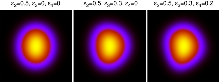
Figure 1: Heat map of $s$ values in the transverse plane, with multiple superimposed symmetries. The more $\epsilon_{N}$ components are included, the more asymmetric the shape gets.

We also calculated hadronic observables from the above solution (see details of the freeze-out scenario in Ref [3] or Ref. [5]. A comparison to PHENIX data on higher order harmonics measured in 200 GeV Au+Au collisions [6] is shown in Fig. 2. Fit parameters of the model are $\epsilon_{N}$ (for $N=2,3,4$), $u_{t}$ and $b$ ($T_{0}$ and $\tau_{0}$ was fixed to values given from spectra and HBT comparisons of a similar model, as described in Refs. [3, 5]).

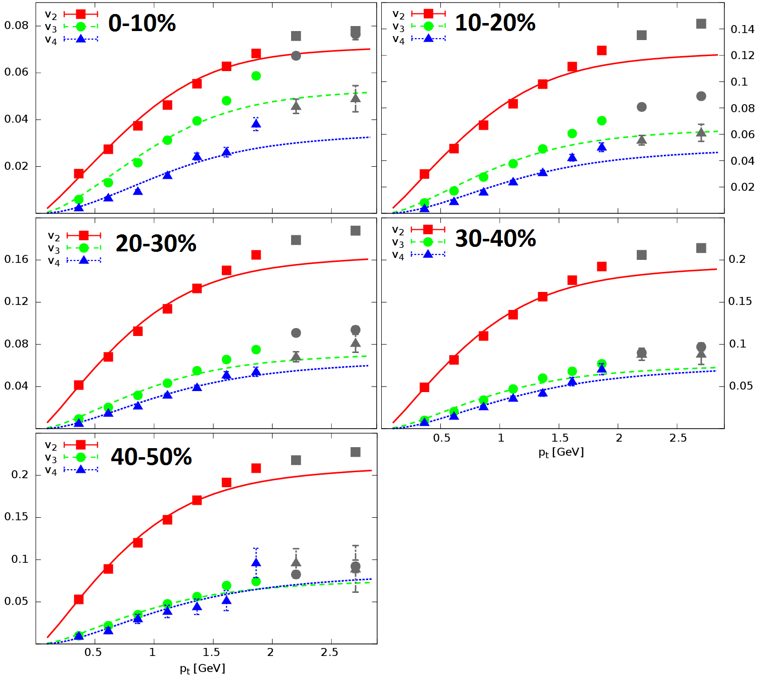
Figure 2: Fits to PHENIX 200 GeV Au+Au data [6] in 5 centrality bins. Fit parameters are summarized in Ref. [3]

3 Time evolution of the anisotropies

In the above described solution, the anisotropies don’t change over time - due to the lack of pressure gradients and the Hubble-flow. In a numerical framework, we investigated how the introduction of pressure gradients, various speeds of sound and viscosity coefficients influence the time evolution of the asymmetries, when starting from an initial condition that is very similar to one described by know analytic solutions – except in pressure, where we used a pressure profile similar to the density profile given in usual Hubble-expansion models [4, 3]. We used a multi-stage predictor-corrector method outlined in Ref. [7]. This is a finite volume scheme, where the initial flux is a weighted average of the Lax-Friedrichs and Lax-Wendroff fluxes, called GFORCE. This flux is used to make a new prediction on the grid points, which is used to get a better flux approximation. This procedure is repeated for a number of times, as described e.g. in Ref. [7]. This multi-stage flux gives results that are comparable to those of the Godunov method. We tested our method with known analytic solutions given in Refs. [8, 4, 3]. We analyzed both non-relativistic and relativistic hydrodynamics, and arrived at similar conclusions.

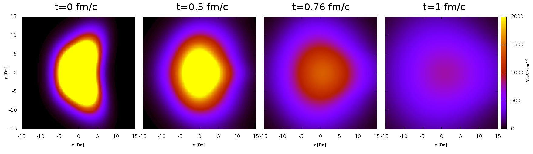
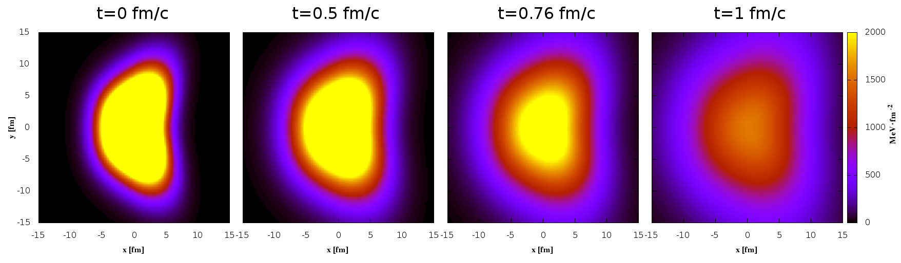
Figure 3: Time evolution of energy density. Top row shows viscosity free case, the bottom row with $\mu={\rm 10MeV}\cdot{\rm fm}$ viscosity.

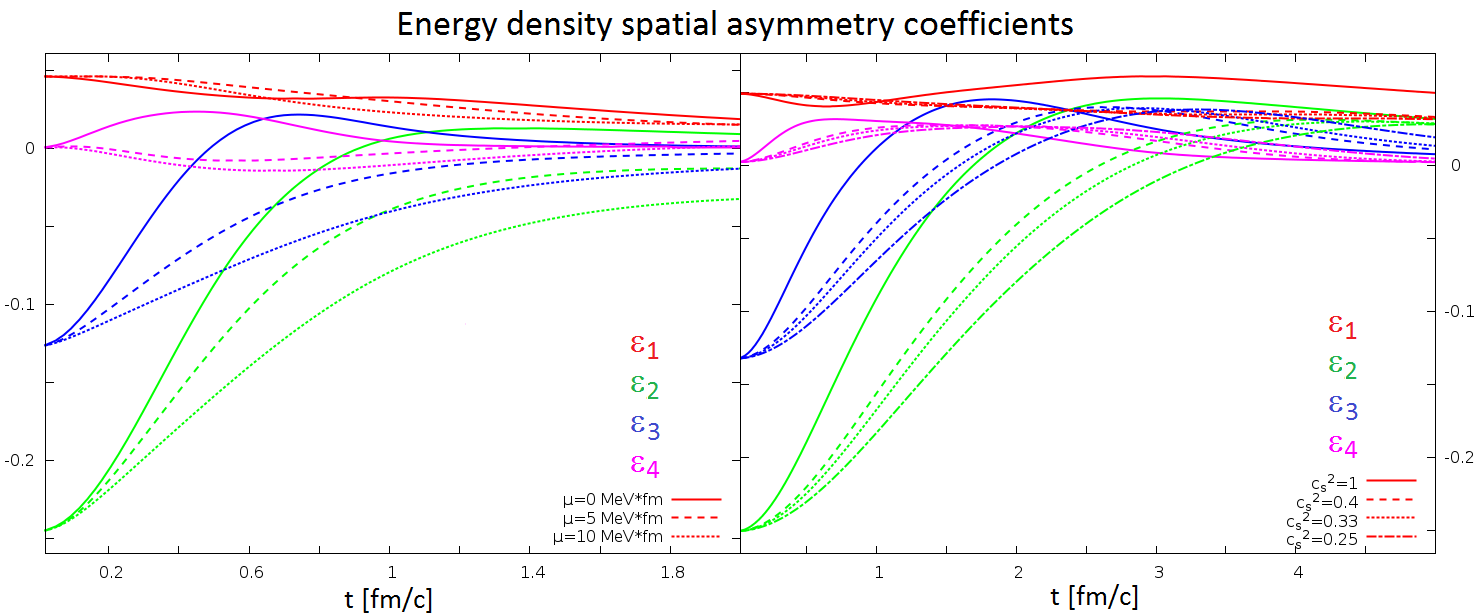
Figure 4: The time evolution of the asymmetry coefficients $\epsilon_{1,2,3,4}$ in the energy density, as modified by a small amount of viscosity (left plot) and the change in speed of sound (right plot).

Fig. 3 shows the result of a nonrelativistic calculation of the time evolution of the energy density. If we assume a small amount of viscosity, it makes the flow itself and thus the disappearance of asymmetries slower. The time evolution of the asymmetries themselves is shown in Fig. 4. In this figure we also see the effect of speed of sound in this nonrelativistic calculation: the reduction of speed of sound makes the asymmetries disappear slower – due to the reduction of the speed of sound waves. A similar effect is seen in case of a relativistic calculation, as shown in Fig. 5: the increase of $\kappa=c_{s}^{-2}$ makes the disappearance of asymmetries slower. It is important to see that this also slows down the speed of cooling, which means the system will freeze out latter.

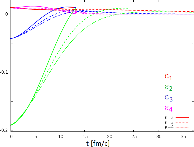
Figure 5: The time evolution of the asymmetry coefficients in the energy density in a relativistic calculation, as modified by the change in $\kappa=c_{s}^{-2}$ (right plot).

4 Anisotropy mixing

It is important to see that there may be asymmetries in both momentum space (i.e. in the velocity field) and in density (i.e. in energy density or pressure), and both influence the measured anisotropies. To investigate this effect, we created a multipole version of the Buda-Lund model [9], with a scale variable given in Eq. 3, but we introduced a multipole flow field as well. We start from a “flow potential” $\Phi$, which gives us the flow:

$${\bf v}=(\partial_{x}\Phi,\partial_{y}\Phi,\partial_{z}\Phi).$$ (7)

The flow field at a given time is spherically symmetric if $\Phi=\frac{r^{2}}{2H}$ with $H$ being a Hubble-coefficient at that given time. Elliptical symmetry is obtained with $\Phi=\frac{r^{2}}{2H}(1+\chi_{2}\cos(2\varphi))$, while

$$\Phi=\frac{r^{2}}{2H}(1+\chi_{2}\cos(2\varphi))+\frac{r^{3}}{3H^{2}}\chi_{3}\cos(3\varphi))$$ (8)

represents a triangular perturbation of the elliptical flow. Of course the various anisotropies can have various event planes (symmetry planes), but the specific angle of these does not enter into the results. Inspired by Ref. [10], we analyzed how $\chi_{2,3}$ and $\epsilon_{2,3}$ influence flow coefficients $v_{2}$ and $v_{3}$ – see results in Fig. 6. Compared to the spatial anisotropy, velocity field anisotropy has a much larger effect on elliptic and triangular flow coefficients.

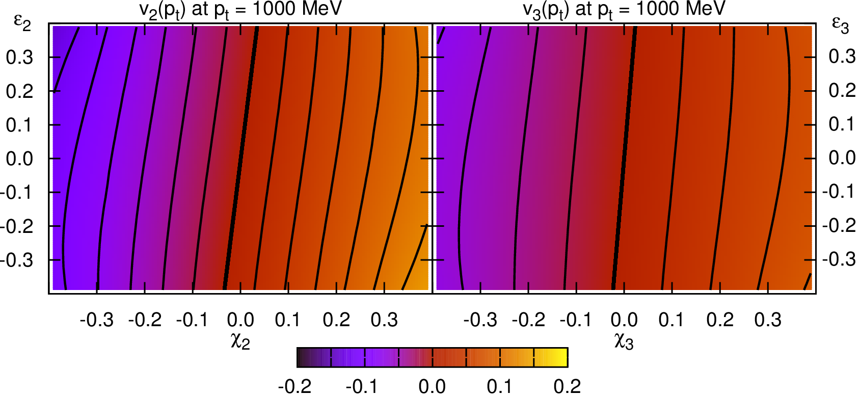
Figure 6: Dependence of flow anisotropy coefficients $v_{2,3}$ on asymmetry parameters $\chi_{2,3}$ and $\epsilon_{2,3}$. Velocity field asymmetry has a stronger influence on flow coefficients.

5 Summary and acknowledgments

In this paper we showed an extension of the scope of analytic relativistic hydrodynamics to higher order azimuthal asymmetries, compatible with realistic (event-by-event fluctuating) geometries. Higher order flow observables were calculated from this model, and are found to be compatible with data. In the analytic model, anisotropy parameters were independent of time, thus we investigated their time evolution in a numerical framework, developed for this purpose. We also investigated how velocity- and density-field anisotropies “mix”, in the framework of a multipole Buda-Lund model. We are thankful to Tam s Cs rg and M rton Nagy for useful discussions with respect to this project. We thank the WPCF community and the WPCF 2014 organizers, in particular the local hosts, Tam s Nov k and Tam s Cs rg , for the possibility to present this work. We also thankfully acknowledge the support of the OTKA grant NK 101438.

References

- [1] R. Chatterjee, D. K. Srivastava, and T. Renk arXiv:1401.7464 [hep-ph].
- [2] L. Yan and J.-Y. Ollitrault Phys.Lett. B744 (2015) 82–87, arXiv:1502.02502 [nucl-th].
- [3] M. Csanád and A. Szabó Phys.Rev. C90 no. 5, (2014) 054911, arXiv:1405.3877 [nucl-th].
- [4] T. Csörgő, L. P. Csernai, Y. Hama, and T. Kodama Heavy Ion Phys. A21 (2004) 73–84, nucl-th/0306004.
- [5] M. Csanád and M. Vargyas Eur. Phys. J. A44 (2010) 473–478, arXiv:0909.4842 [nucl-th].
- [6] A. Adare et al. Phys.Rev.Lett. 107 (2011) 252301, arXiv:1105.3928 [nucl-ex].
- [7] E. F. Toro and V. A. Titarev J. Comp. Phys. 216 (2016) 403–429.
- [8] T. Csörgő, S. V. Akkelin, Y. Hama, B. Lukács, and Y. M. Sinyukov Phys. Rev. C67 (2003) 034904, hep-ph/0108067.
- [9] M. Csanád, T. Csörgő, and B. Lörstad Nucl. Phys. A742 (2004) 80–94, nucl-th/0310040.
- [10] M. Csanád, B. Tomásik, and T. Csörgő Eur. Phys. J. A 37 (2008) 111–119, arXiv:0801.4434 [nucl-th].