• We consider the spectrum of correlation lengths of the spin-$\frac{1}{2}$ XXZ chain in the antiferromagnetic massive regime. These are given as ratios of eigenvalues of the quantum transfer matrix of the model. The eigenvalues are determined by integrals over certain auxiliary functions and by their zeros. The auxiliary functions satisfy nonlinear integral equations. We analyse these nonlinear integral equations in the low-temperature limit. In this limit we can determine the auxiliary functions and the expressions for the eigenvalues as functions of a finite number of parameters which satisfy finite sets of algebraic equations, the so-called higher-level Bethe Ansatz equations. The behaviour of these equations, if we send the temperature $T$ to zero, is different for zero and non-zero magnetic field $h$. If $h$ is zero the situation is much like in the case of the usual transfer matrix. Non-trivial higher-level Bethe Ansatz equations remain which determine certain complex excitation parameters as functions of hole parameters which are free on a line segment in the complex plane. If $h$ is non-zero, on the other hand, a remarkable restructuring occurs, and all parameters which enter the description of the quantum transfer matrix eigenvalues can be interpreted entirely in terms of particles and holes which are freely located on two curves when $T$ goes to zero.
  PACS: 05.30.-d, 75.10.Pq

1 Introduction

The quantum transfer matrix formalism [25, 26] provides a framework for calculating the thermodynamic properties [24, 16] and correlation functions [8, 9, 5, 6] of integrable lattice models analytically. It enables, in particular, the calculation of correlation lengths of integrable Heisenberg chains [15, 16, 27, 17, 18] and related Fermion models [23].

The main concern of this work is the calculation of the full spectrum of correlation lengths of the XXZ chain in the antiferromagnetic massive regime at finite magnetic field $h$ and low temperature $T$, i.e. for large ratios $h/T$. The above cited previous works dealt with the massless regime or with the case that $h/T$ is small and were mainly restricted to the calculation of a few largest correlation lengths. Our study is the first step in the analysis of the low-temperature behaviour of two-point correlation functions, especially of their large-distance asymptotics, by means of a form factor approach, as, in fact, a form factor expansion requires the summation over a complete set of intermediate states.

A form-factor based analysis of the large-distance asymptotics of two-point functions at low temperatures was recently completed for the model in the massless (or critical) regime [5, 6]. In that work, as well as in the previous analysis of ground-state correlation functions within a form-factor approach [12, 14, 13], a finite magnetic field turned out to be an important regularization parameter. As long as the magnetic field is finite, the low-energy excitations above the ground state can be classified as particle-hole excitations about two Fermi points, and a similarly simple picture holds for the ‘excitations’ of the quantum transfer matrix as well. When sending first $T$ and then $h$ to zero we found numerical agreement of our formulae for the correlation amplitudes [6] with the explicit formulae obtained by Lukyanov [21] for the ground state at vanishing magnetic field.

It is our hope that a similar program can be carried out in the massive regime and that we will be able to obtain even more explicit results in terms of certain special functions. This can be expected, since there are no Fermi points in the massive regime and since the functions that enter naturally into the description of correlation functions are periodic or quasi-periodic with period or quasi-period $\pi$. In fact, in some cases the multiple-integral formulae for the form factors of the XXZ chain in the antiferromagnetic massive regime at zero temperature and magnetic field, that were obtained within the vertex-operator approach [10, 20, 22], could be evaluated in closed form.

More recently we considered form factors of the usual transfer matrix in the antiferromagnetic massive regime from a Bethe Ansatz perspective [7]. In this case the ground state magnetization is zero, and the excitations are characterized by Bethe root patterns that involve non-real roots, organized in so-called wide pairs and two-strings satisfying a set of ‘higher-level’ Bethe Ansatz equations [30, 28, 2]. These remain non-trivial even in the thermodynamic limit. The appearance of the higher-level Bethe Ansatz equations as well as the singular behaviour in the thermodynamic limit of norms of Bethe states involving two-strings made the analysis rather delicate. In the end we obtained novel formulae for the form factors in the thermodynamic limit for which we found numerical agreement with rather differently looking formulae obtained within the vertex operator approach [20, 22].

As we shall see below, in the limit $T\rightarrow 0_{+}$ the Bethe roots which determine the spectrum of the quantum transfer matrix at vanishing magnetic field satisfy a set of higher-level Bethe Ansatz equations of the same form as in case of the usual transfer matrix. If the magnetic field is non-zero however, we observe a dramatic reorganization of the Bethe root patterns at low temperatures. Like in the massless case it turns out to be possible to interpret them entirely in terms of particle-hole excitations. At small finite temperatures the positions of the particle and hole parameters in the complex plane are still determined by a set of higher-level Bethe Ansatz equations. But as the temperature goes to zero they become free parameters on two branches of a curve in the complex plane. The eigenvalue ratios, which determine the correlation lengths, are explicit functions of these parameters. This is the main result of this work. It will lead to yet another form factor series for the ground state two-point functions of the XXZ chain in the thermodynamic limit. We shall report it in a separate publication.

The paper is organized as follows. In the remaining part of this introduction we recall the Hamiltonian and its ground state phase diagram. We also recall the expansion of thermal correlation functions in terms of eigenstates and eigenvalues of the quantum transfer matrix. The main subject of this work, which is the calculation of the spectrum of correlation lengths of the XXZ chain in the massive antiferromagnetic regime at finite magnetic field for low temperatures, is then explored in section 2 and followed by conclusions in section 3. Appendix 3 contains a summary of the properties of the basic functions that determine the low-temperature behaviour of the correlation lengths, namely, the dressed momentum, dressed energy and dressed phase which, in the massive antiferromagnetic regime, can be explicitly expressed in terms of elliptic functions and $q$-Gamma functions. Appendix A.3 contains important complementary material on the numerical study of the Bethe Ansatz equations and of the eigenvalues of the quantum transfer matrix at finite Trotter number.

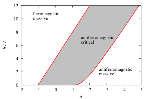
Figure 1: The ground state phase diagram of the XXZ chain in the $\Delta$-$h$ plane.

1.1 Hamiltonian and ground state phase diagram

The Hamiltonian of the spin-$\frac{1}{2}$ XXZ chain in a homogeneous magnetic field parallel to the direction of its anisotropy axis may be written as

$$H=J\sum_{j=-L+1}^{L}\Bigl{(}\sigma_{j-1}^{x}\sigma_{j}^{x}+\sigma_{j-1}^{y}\sigma_{j}^{y}+\Delta\bigl{(}\sigma_{j-1}^{z}\sigma_{j}^{z}-1\bigr{)}\Bigr{)}-\frac{h}{2}\sum_{j=-L+1}^{L}\sigma_{j}^{z}\,,$$ (1)

where the $\sigma_{j}^{\alpha}$ are Pauli matrices $\sigma^{\alpha}$ acting on the $j$th factor of the tensor-product space of states ${\cal H}={\mathbb{C}}^{\otimes 2L}$ of $2L$ spins $\frac{1}{2}$. We choose the number of spins in the chain to be even, since this implies that the ground state of the Hamiltonian (1) is unique for $h=0$, $\Delta>-1$ and every $L\in 2{\mathbb{N}}$. Below we will consider the system in the thermodynamic limit $L\rightarrow\infty$ and at finite temperature $T$. The Hamiltonian (1) depends on three parameters, the strength of the exchange interaction, $J>0$, which sets the energy scale, the strength of the magnetic field, $h\geq 0$, and the anisotropy parameter $\Delta$.

The ground state phase diagram in the $\Delta$-$h$ parameter plane was obtained by Yang and Yang [31] (see Figure 1). For $\Delta>1$ the zero-temperature magnetization vanishes below a lower critical field $h_{\ell}$ (right red line in Figure 1). This region of the $\Delta$-$h$ parameter plane is called the antiferromagnetic massive regime. It contains the Ising chain ($h=0$, $\Delta=+\infty$) as a particular point. The physical properties of the model in the antiferromagnetic massive regime are believed to be approximately accessible by perturbation theory around the Ising limit ($\Delta\rightarrow+\infty$). The ground state in this regime becomes two-fold degenerate in the thermodynamic limit, and the lowest excited states are separated from the degenerate ground states by a finite energy gap (or ‘mass gap’). The two degenerate ground states in the thermodynamic limit may be thought of as ‘finite-$\Delta$ deformations’ of the two Néel states which are the ground states of the Ising chain.

1.2 Correlation functions and correlation lengths by Bethe Ansatz

In this work we study the model in the antiferromagnetic massive regime non-perturbatively, using its integrable structure encoded in the $R$-matrix

$$\begin{array}[]{cc}R(x,y)=\begin{pmatrix}1&0&0&0\\ 0&b(x,y)&c(x,y)&0\\ 0&c(x,y)&b(x,y)&0\\ 0&0&0&1\end{pmatrix}\,,&\begin{array}[]{c}b(x,y)=\frac{\sin(y-x)}{\sin(y-x+{\rm i}\gamma)}\\[8.61108pt] c(x,y)=\frac{\sin({\rm i}\gamma)}{\sin(y-x+{\rm i}\gamma)}\end{array}\end{array}\,,$$ (2)

of the six-vertex model. As is well known [3] the Hamiltonian (1) at $h=0$ is proportional to the logarithmic derivative of the transfer matrix of the homogeneous six-vertex model. Its anisotropy parameter $\Delta$ is then a function of the deformation parameter $\gamma$ of the $R$-matrix, $\Delta=\operatorname{ch}(\gamma)$. In the antiferromagnetic massive regime $\gamma$ must be real. In the following we restrict ourselves to $\gamma>0$. Later on we shall also use the common notation $q={\rm e}^{-\gamma}$.

For the calculation of temperature correlation functions and their correlation lengths we need the statistical operator ${\rm e}^{-H/T}$ rather than the Hamiltonian. This operator can be related to the monodromy matrix of an inhomogeneous auxiliary six-vertex model defined for every lattice site $j\in\{-L+1,\dots,L\}$ by

$$T_{j}(x)=q^{\kappa\sigma_{j}^{z}}R_{j\overline{N}}\bigl{(}x,{\textstyle\frac{{\rm i}\beta}{N}}\bigr{)}R_{\overline{N-1}j}^{t_{1}}\bigl{(}-{\textstyle\frac{{\rm i}\beta}{N}},x\bigr{)}\dots R_{j\overline{2}}\bigl{(}x,{\textstyle\frac{{\rm i}\beta}{N}}\bigr{)}R_{\bar{1}j}^{t_{1}}\bigl{(}-{\textstyle\frac{{\rm i}\beta}{N}},x\bigr{)}\,.$$ (3)

Here $N\in 2{\mathbb{N}}$ is called the Trotter number, and the indices $\bar{j}=\bar{1},\dots,\overline{N}$ refer to $N$ auxiliary sites in ‘Trotter direction’. Furthermore

$$\beta=-\frac{2J\operatorname{sh}(\gamma)}{T}\,,\qquad\kappa=-\frac{h}{2\gamma T}$$ (4)

are rescaled inverse temperature and magnetic field.

Define

$$\rho_{N,L}=\operatorname{Tr}_{\bar{1}\dots\overline{N}}\{T_{-L+1}(0)\dots T_{L}(0)\}\,.$$ (5)

Then it is easy to see [8] that

$${\rm e}^{-H/T}=\lim_{N\rightarrow\infty}\rho_{N,L}\,.$$ (6)

We call $\rho_{N,L}$ a finite Trotter number approximant of the statistical operator. Using $\rho_{N,L}$ we obtain simple expressions for the finite Trotter number approximants of correlation functions. Namely, for any product of local operators ${\cal O}^{(j)}\in\operatorname{End}{\mathbb{C}}^{2}$, $j=1,\dots,m$, acting on $m$ consecutive sites

$$\bigl{\langle}{\cal O}_{1}^{(1)}\dots\cal O_{m}^{(m)}\bigr{\rangle}_{N}=\lim_{L\rightarrow\infty}\frac{\operatorname{Tr}_{-L+1\dots L}\bigl{\{}\rho_{N,L}{\cal O}_{1}^{(1)}\dots\cal O_{m}^{(m)}\bigr{\}}}{\operatorname{Tr}_{-L+1\dots L}\{\rho_{N,L}\}}\\[6.45831pt] =\frac{\langle\Psi_{0}|\operatorname{Tr}\{{\cal O}^{(1)}T(0)\}\dots\operatorname{Tr}\{{\cal O}^{(m)}T(0)\}|\Psi_{0}\rangle}{\langle\Psi_{0}|\Psi_{0}\rangle\Lambda_{0}^{m}(0)}\,,$$ (7)

where $\Lambda_{0}(0)$ is the unique eigenvalue of largest modulus of the quantum transfer matrix $t(\lambda)=\operatorname{Tr}T(\lambda)$ at $\lambda=0$, and where $|\Psi_{0}\rangle$ is the corresponding eigenvector (see [8] for more details). The other eigenstates will be denoted $|\Psi_{n}\rangle$, the associated eigenvalues $\Lambda_{n}(\lambda)$.

Replacing $m$ by $m+1$ in (7) and considering e.g. ${\cal O}^{(1)}=\sigma^{-}$, ${\cal O}^{(m+1)}=\sigma^{+}$ and the intermediate operators to be unity, we obtain a finite temperature asymptotic expansion for the transverse correlation functions,

$$\langle\sigma_{1}^{-}\sigma_{m+1}^{+}\rangle_{N}=\sum_{n}A_{n}^{-+}\rho_{n}^{m}\,,$$ (8)

if we insert a complete set of states. Here we have used the notation

$$\rho_{n}={\rm e}^{-1/\xi_{n}}=\frac{\Lambda_{n}(0)}{\Lambda_{0}(0)}\,,\quad A_{n}^{-+}=\frac{\langle\Psi_{0}|T^{1}_{2}(0)|\Psi_{n}\rangle}{\Lambda_{n}(0)\langle\Psi_{0}|\Psi_{0}\rangle}\,\frac{\langle\Psi_{n}|T^{2}_{1}(0)|\Psi_{0}\rangle}{\Lambda_{0}(0)\langle\Psi_{n}|\Psi_{n}\rangle}\,.$$ (9)

Similar expansions hold for the longitudinal two-point functions and for their generating function [5]. The sum on the right hand side of (8) is finite as long as the Trotter number is finite. In the Trotter limit $N\rightarrow\infty$ it turns into a series that provides an easy access to the large-distance asymptotic behaviour of the thermal correlation function $\langle\sigma_{1}^{-}\sigma_{m+1}^{+}\rangle$, since $|\rho_{n}|<1$ for $n\in{\mathbb{Z}}_{+}$. The $\rho_{n}$ are ratios of higher eigenvalues of the quantum transfer matrix to the dominant eigenvalue $\Lambda_{0}$. The specific choice of the operators in (7) ($\sigma^{-}$, $\sigma^{+}$ in our example (8)) determines which amplitudes will be non-zero and, hence, which eigenvalue ratios will appear. The numbers $\xi_{n}$ are called the correlation lengths. They are generally non-real and describe the rate of exponential decay with distance of a given term in the series (8) as well as its oscillatory behaviour. The coefficients $A_{n}^{-+}$ are called correlation amplitudes. They are products of two factors which we called thermal form factors in [5].

In this work we analyse the low-temperature behaviour of the eigenvalue ratios $\rho_{n}$ in the massive regime, i.e. we concentrate on the spectrum of the quantum transfer matrix. An exploration of the low-temperature properties of the correlation amplitudes for the transverse and longitudinal correlation functions as well as of the behaviour of the corresponding series representations of two-point functions is deferred to a separate publication.

For any finite Trotter number the eigenvalues of the quantum transfer matrix are determined by the algebraic Bethe Ansatz (see e.g. [8]):

$$\Lambda(x)={\rm e}^{\frac{h}{2T}}\biggl{(}\frac{\sin(x+{\rm i}\beta/N)}{\sin(x+{\rm i}\beta/N+{\rm i}\gamma)}\biggr{)}^{\frac{N}{2}}\biggl{[}\prod_{j=1}^{M}\frac{\sin(x-x_{j}^{r}+{\rm i}\gamma/2)}{\sin(x-x_{j}^{r}-{\rm i}\gamma/2)}\biggr{]}\bigl{(}1+\mathfrak{a}(x-{\rm i}\gamma/2)\bigr{)}\,,$$ (10)

where the auxiliary function $\mathfrak{a}$ is defined by

$$\mathfrak{a}(x)=\mathfrak{a}\bigl{(}x\big{|}\{x_{k}^{r}\}_{k=1}^{M}\bigr{)}\\ ={\rm e}^{-\frac{h}{T}}\biggl{(}\frac{\sin(x+{\rm i}\gamma/2-{\rm i}\beta/N)\sin(x+3{\rm i}\gamma/2+{\rm i}\beta/N)}{\sin(x+{\rm i}\gamma/2+{\rm i}\beta/N)\sin(x-{\rm i}\gamma/2-{\rm i}\beta/N)}\biggr{)}^{\frac{N}{2}}\prod_{k=1}^{M}\frac{\sin(x-x_{k}^{r}-{\rm i}\gamma)}{\sin(x-x_{k}^{r}+{\rm i}\gamma)}.$$ (11)

and where the Bethe roots $x_{j}^{r}$ are subject to the Bethe Ansatz equations

$$\mathfrak{a}\bigl{(}x_{j}^{r}\big{|}\{x_{k}^{r}\}_{k=1}^{M}\bigr{)}=-1\,,\quad j=1,\dots,M\,.$$ (12)

Throughout this work we shall assume that the Bethe roots $x_{j}^{r}$ are pairwise distinct. This is not a severe limitation in that, should some of the roots coincide, it would be enough to slightly deform the auxiliary function $\mathfrak{a}$ (and thus the Bethe Ansatz equations) by introducing additional ‘deformation parameters’, then perform the analysis of the equations and send the deformation parameters to zero in the end.

At this point we can formulate our goal on a technical level: we want to analyse equations (10)-(12) in the Trotter limit for small $T$, for $h$ below the lower critical field, and for fixed value of the ‘spin’

$$s=N/2-M\,.$$ (13)

Note that $s=0$ for the longitudinal two-point functions, while $s=1$ for the transverse two-point functions (8). Spin $s=-1$ belongs to the transverse two-point function $\langle\sigma_{1}^{+}\sigma_{m+1}^{-}\rangle$, while larger values of $|s|$ occur in the study of multi-point correlation functions or if we study higher form factors with several local operators acting on neighbouring sites. Instead of the Bethe Ansatz equations (12) and the defining equation (11) we shall introduce an equivalent characterization of the auxiliary function $\mathfrak{a}$ by means of a nonlinear integral equation in the next section. Using the nonlinear integral equation we can easily perform the Trotter limit and also get access to the low-temperature limit in which the nonlinear integral equation linearizes.

2 Low-temperature spectrum of correlation lengths

2.1 Nonlinear integral equation for the auxiliary function

The nonlinear integral equation will connect $\ln\mathfrak{a}$ and $\ln(1+\mathfrak{a})$. As we shall see, in the antiferromagnetic massive regime it turns out to be important to keep control over the overall phase of the logarithms. For taking the logarithm of equation (11) we introduce for every $\delta>0$ the functions

$$K(x|\delta)=\frac{1}{2\pi{\rm i}}\bigl{(}\,{\rm ctg}\,(x-{\rm i}\delta)-\,{\rm ctg}\,(x+{\rm i}\delta)\bigr{)}\,,$$ (14a)

$$\theta(x|\delta)=2\pi{\rm i}\int_{\Gamma_{x}}{\rm d}y\>K(y|\delta)\,,$$ (14b)

where $\Gamma_{x}$ is a piecewise straight contour starting at $-\pi/2$, running parallel to the imaginary axis to $-\pi/2+{\rm i}\,{\rm Im\,}x$ and then parallel to the real axis from $-\pi/2+{\rm i}\,{\rm Im\,}x$ to $x$. Accordingly, the function $\theta(x|\delta)$ is defined in the cut complex plane with cuts along the line segments $(-\infty\pm{\rm i}\delta,-\pi\pm{\rm i}\delta]\cup[\pm{\rm i}\delta,\pm{\rm i}\delta+\infty)$. If $\delta=\gamma$ we shall write $K(x)=K(x|\gamma)$ and $\theta(x)=\theta(x|\gamma)$ for short.

Hereafter we will use the following properties of these functions:

$$K(x|\delta)=\frac{1}{2\pi}\,\frac{\operatorname{sh}(2\delta)}{\operatorname{sh}^{2}(\delta)+\sin^{2}(x)}>0\,,\quad\text{for $x\in{\mathbb{R}}$,}$$ (15a)

$$K(x+\pi|\delta)=K(x|\delta)\,,\quad K(-x|\delta)=K(x|\delta)\,,$$ (15b)

$$\theta(x+\pi|\delta)=\theta(x|\delta)+\begin{cases}2\pi{\rm i}&|{\rm Im\,}x|<\delta\\ 0&|{\rm Im\,}x|>\delta,\end{cases}$$ (15c)

$$\theta(-x|\delta)=-\theta(x|\delta)+\begin{cases}2\pi{\rm i}&|{\rm Im\,}x|<\delta\\ 0&|{\rm Im\,}x|>\delta.\end{cases}$$ (15d)

It follows from (15c) and (15d) that $\theta(\pi/2|\delta)=2\pi{\rm i}$ and $\theta(0|\delta)=\pi{\rm i}$. Setting $x=u+{\rm i}v$, $u,v\in{\mathbb{R}}$ we further find the asymptotic behaviour

$$\lim_{v\rightarrow\pm\infty}\theta(u+{\rm i}v)=\mp 2\gamma\,.$$ (16)

Note that $\theta(x|\delta)$ is a determination of the logarithm of $\sin(x-{\rm i}\delta)/\sin(x+{\rm i}\delta)$ which coincides with its principle branch $\operatorname{Ln}\bigl{(}\sin(x-{\rm i}\delta)/\sin(x+{\rm i}\delta)\bigr{)}$ in the strip $-\pi<{\rm Re\,}x<\nolinebreak 0$. Here and in the following we define the latter in such a way that $-\pi<{\rm Im\,}\operatorname{Ln}(x)\leq\pi$.

Using $\theta$ in (11) we can define the function $\ln\mathfrak{a}$ as

$$\ln\mathfrak{a}(x)=-\frac{\varepsilon_{0}^{(N)}(x)}{T}-\frac{N}{2}\theta(x+{\rm i}\gamma/2+{\rm i}\beta/N)+\sum_{j=1}^{M}\theta(x-x_{k}^{r})\,,$$ (17)

where

$$\varepsilon_{0}^{(N)}(x)=h-\frac{NT}{2}\bigl{[}\theta(x+{\rm i}\beta/N|\gamma/2)-\theta(x-{\rm i}\beta/N|\gamma/2)\bigr{]}\,.$$ (18)

Starting from this equation we may derive an integral equation for $\mathfrak{a}$. The form of this integral equation will depend on our initial choice of the integration contour. We choose a rectangular, positively oriented contour ${\cal C}$ starting and ending at $-\pi/2$ and defined in such a way that its upper edge ${\cal C}_{+}$ joins $\pi/2$ with $-\pi/2$ while its lower edge ${\cal C}_{-}$ joins $-\pi/2-{\rm i}\gamma^{-}$ with $\pi/2-{\rm i}\gamma^{-}$. We further denote its left edge by ${\cal C}_{\ell}$ and its right edge by ${\cal C}_{r}$. By definition $\gamma^{-}=\gamma-0_{+}$.

Figure 2: The integration contour ${\cal C}$.

Relative to the contour $\cal C$ we introduce the following terminology for the roots of the equation

$$1+\mathfrak{a}(x)=0\,.$$ (19)

A root $x$ of (19) is called a Bethe root if $x\in\{x_{k}^{r}\}_{k=1}^{M}$. Bethe roots outside $\cal C$ are called particle roots or particles. A particle $x$ is called close if $x-{\rm i}\gamma$ is inside $\cal C$, far otherwise. We denote the number of close particles $n_{c}$ and the number of far particles $n_{f}$. The close and far particles themselves will be denoted $x_{j}^{c}$ and $x_{k}^{f}$. Roots of (19) inside $\cal C$ other than Bethe roots are called holes. They are denoted $x_{j}^{h}$ while their number is $n_{h}$ by definition.

It follows from (15c) and (17) that, for real $x$ and $|\beta/N|<\gamma/2$,

$$\ln\mathfrak{a}(x+\pi)=\ln\mathfrak{a}(x)-2\pi{\rm i}(s+n_{f})\,.$$ (20)

Similarly, using (16) in (17) we conclude that

$$\lim_{{\rm Im\,}x\rightarrow\pm\infty}\ln\mathfrak{a}(x)=-\frac{h}{T}\pm 2\gamma s\,.$$ (21)

The functions $\mathfrak{a}$ and $1+\mathfrak{a}$ are meromorphic and have the same poles inside the strip $-\pi/2<{\rm Im\,}x\leq\pi/2$: two $N/2$-fold poles at $\pm{\rm i}(\gamma/2+\beta/N)$ and $M$ simple poles at $x_{k}^{r}-{\rm i}\gamma$ (note that we assume that all roots of (19) are simple). It follows that the only singularities of $\partial_{x}\ln(1+\mathfrak{a}(x))=\mathfrak{a}^{\prime}(x)/(1+\mathfrak{a}(x))$ inside $\cal C$ are the simple poles:

location	residue
$x\in\{x_{k}^{r}\}_{k=1}^{M}\setminus\bigl{\{}\{x_{k}^{c}\}_{k=1}^{n_{c}}\cup\{x_{k}^{f}\}_{k=1}^{n_{f}}\bigr{\}}$	$1$
$x\in\{x_{k}^{h}\}_{k=1}^{n_{h}}$	$1$
$x\in\{x_{k}^{c}-{\rm i}\gamma\}_{k=1}^{n_{c}}$	$-1$
$x=-{\rm i}(\gamma/2+\beta/N)$	$-N/2$

Moreover, if $x,y\in{\cal C}$ or inside, then $\theta(x-y)$ is holomorphic as a function of $y$. It follows that, for $-\gamma<{\rm Im\,}(x)<0$,

$$\ln\mathfrak{a}(x)=-\frac{\varepsilon_{0}^{(N)}(x)}{T}-\sum_{j=1}^{n_{h}}\theta(x-x_{j}^{h})+\sum_{j=1}^{n_{c}}\bigl{(}\theta(x-x_{j}^{c})+\theta(x-x_{j}^{c}+{\rm i}\gamma)\bigr{)}+\sum_{j=1}^{n_{f}}\theta(x-x_{j}^{f})\\ +\int_{\cal C}\frac{{\rm d}y}{2\pi{\rm i}}\theta(x-y)\partial_{y}\ln(1+\mathfrak{a}(y))\,.$$ (22)

This equation can be transformed into a nonlinear integral equation for the auxiliary function by partial integration. Again some care is necessary with the definition of the logarithms. First of all, there is no ambiguity in the definition of the function $\partial_{x}\ln(1+\mathfrak{a}(x))$ which is simply defined as $\mathfrak{a}^{\prime}(x)/(1+\mathfrak{a}(x))$, similarly $\partial_{x}\ln\mathfrak{a}(x)=\mathfrak{a}^{\prime}(x)/\mathfrak{a}(x)$ by definition. For any point $x$ on $\cal C$ and $f=\mathfrak{a},1+\mathfrak{a},1+\mathfrak{a}^{-1}$ we now define

$$\ln_{\cal C}f(x)=\int_{{\cal C}_{x}}{\rm d}y\>\partial_{y}\ln f(y)\,.$$ (23)

Here ${\cal C}_{x}$ is the simple contour which starts at $-\pi/2-{\rm i}0$ and runs along ${\cal C}$ up to the point $x$. The function $\ln_{\cal C}f$ is holomorphic along ${\cal C}$ by construction and can be used in partial integration. The monodromy of $\ln_{\cal C}(1+\mathfrak{a})(x)$ along ${\cal C}$ is generally nontrivial. Using the above tabular we find that

$$d=\int_{\cal C}\frac{{\rm d}y}{2\pi{\rm i}}\partial_{y}\ln(1+\mathfrak{a}(y))=\frac{\ln_{\cal C}(1+\mathfrak{a})(-\pi/2)}{2\pi{\rm i}}=n_{h}-2n_{c}-n_{f}-s$$ (24)

which may be generally non-zero. Performing now the partial integration in (22) we arrive at the following

Lemma 1.

The auxiliary function $\mathfrak{a}$ defined in (11) satisfies the nonlinear integral equation

$$\ln\mathfrak{a}(x)=-\frac{\varepsilon_{0}^{(N)}(x)}{T}-\sum_{j=1}^{n_{h}}\theta(x-x_{j}^{h})+\sum_{j=1}^{n_{c}}\bigl{(}\theta(x-x_{j}^{c})+\theta(x-x_{j}^{c}+{\rm i}\gamma)\bigr{)}+\sum_{j=1}^{n_{f}}\theta(x-x_{j}^{f})\\ +d\theta(x+\pi/2)+\int_{\cal C}{\rm d}y\>K(x-y)\ln_{\cal C}(1+\mathfrak{a})(y)\,.$$ (25)

This equation determines $\mathfrak{a}$ directly inside the strip $-\gamma<{\rm Im\,}x<0$ and, by analytic continuation, in the entire complex plane. In particular, for $x\in{\cal C}_{\pm}$ the integral term should be understood as an appropriate boundary value of a Cauchy-like operator.

The particles and holes have to be determined such that they satisfy the subsidiary conditions

$$1+\mathfrak{a}\bigl{(}x_{j}^{h,p,f}\bigr{)}=0$$ (26)

with $x_{j}^{h,p,f}$ in their respective domains of definition.

In equation (25) the Trotter limit is easily performed by substituting $\varepsilon_{0}^{(N)}(x)$ by

$$\varepsilon_{0}(x)=\lim_{N\rightarrow\infty}\varepsilon_{0}^{(N)}(x)=h-\frac{4J(\Delta^{2}-1)}{\Delta-\cos(2x)}\,.$$ (27)

Equation (25) is a good starting point for studying the system numerically or, as we shall see below, analytically in the low-temperature limit. Before moving to the latter subject in the next subsection we wish to add three remarks.

Remark 1.

Equations (24), (25) are compatible with the quasi-periodicity property (20) and with the asymptotic behaviour (21) of $\ln\mathfrak{a}$. In fact, using (15) in (25) we obtain for real $x$

$$\ln\mathfrak{a}(x+\pi)=\ln\mathfrak{a}(x)+2\pi{\rm i}(-n_{h}+2n_{c}+d)$$ (28)

which turns into (20) after inserting (24).

To see the compatibility with the asymptotic behaviour we note the following. Due to the $\pi$-periodicity of the auxiliary function, Bethe roots are only defined modulo $\pi$. If there is a Bethe root with real part $-\pi/2$ it must be identified with the same root shifted by $\pi$, having real part $\pi/2$. Then the contour must be deformed such as to exclude one of the two points, the one with real part $-\pi/2$, say. This can be achieved by infinitesimally shifting the contour to the right which then also can be slightly narrowed. Then the right hand side of (25) determines $\ln\mathfrak{a}(x)$ for ${\rm Re\,}x=-\pi/2+\varepsilon$, $\varepsilon>0$ outside $\cal C$ by analytic continuation, and we can calculate the limit along the line ${\rm Re\,}x=-\pi/2+\varepsilon$ using (16) (which is possible if there is no Bethe root with real part $-\pi/2$ anyway),

$$\lim_{v\rightarrow\infty}\ln\mathfrak{a}(-\pi/2+\varepsilon+{\rm i}v)=-\frac{h}{T}-2\gamma(-n_{h}+2n_{c}+n_{f}+d)\,.$$ (29)

Inserting (24) we see that this is compatible with (21).

Remark 2.

So far we have shown that (11) and (12) imply (24) and (25). It is not difficult to see that the converse is also true. Thus, the two pairs of equations (11), (12) and (24), (25) are equivalent.

Remark 3.

Equations (24), (25) depend on our definition of the contour and on the specific class of solutions we are considering. Let us restrict ourselves for a moment to solutions with $n_{f}=0$, and let us deform the contour ${\cal C}\rightarrow{\cal C}_{s}$ in such a way that the points $x_{j}^{c}-{\rm i}\gamma$ are outside ${\cal C}_{s}$. Suppose further that $d=0$ along ${\cal C}_{s}$. Then (25) turns into

$$\ln\mathfrak{a}(x)=-\frac{\varepsilon_{0}^{(N)}(x)}{T}-\sum_{j=1}^{n_{h}}\theta(x-x_{j}^{h})+\sum_{j=1}^{n_{c}}\theta(x-x_{j}^{c})+\int_{{\cal C}_{s}}{\rm d}y\>K(x-y)\ln_{{\cal C}_{s}}(1+\mathfrak{a})(y)\,.$$ (30)

This equation has the same form as the one we used in the analysis of the massless antiferromagnetic regime for $|\Delta|<1$ [5, 6] (in that case we had an additional term $-{\rm i}\pi s$ which is absorbed into the different definition of the function $\theta$ here). In the massless regime for $\Delta>1$ (when the magnetic field is between lower and upper critical field [31]) equation (30) is an appropriate starting point for the analysis of the low-temperature behaviour of correlation lengths. In this case the relevant ‘excitations’ (leading to correlation lengths that diverge for $T\rightarrow 0$) are characterized by particles and holes $x_{j}^{c}$, $x_{k}^{h}$ very close to two Fermi points $\pm Q$, $Q\in(0,\pi/2)$. The condition $d=0$ can be satisfied by performing a small deformation of the contour in the vicinity of the Fermi points and by lifting up the lower part of the contour. This means that the contour ${\cal C}_{s}$ has to be self-consistently determined in the course of the calculation (see [5, 6]).

2.2 The auxiliary function in the low-temperature limit

For the analysis of the low-temperature behaviour of (25) in the antiferromagnetic massive regime we split the integral over $\cal C$ into contributions from its rectilinear parts ${\cal C}_{\ell},\dots,{\cal C}_{+}$ (see Figure 2),

$$\int_{\cal C}{\rm d}y\>K(x-y)\ln_{\cal C}(1+\mathfrak{a})(y)=\int_{{\cal C}_{+}}{\rm d}y\>K(x-y)\ln_{\cal C}\mathfrak{a}(y)\\ +\bigl{(}\theta(x+\pi/2+{\rm i}\gamma^{-})-\theta(x+\pi/2)\bigr{)}\int_{{\cal C}_{-}}\frac{{\rm d}y}{2\pi{\rm i}}\partial_{y}\ln(1+\mathfrak{a}(y))\\ +\int_{{\cal C}_{+}}{\rm d}y\>K(x-y)\ln_{\cal C}(1+\mathfrak{a}^{-1})(y)+\int_{{\cal C}_{-}}{\rm d}y\>K(x-y)\ln_{\cal C}(1+\mathfrak{a})(y)\,.$$ (31)

Here we have used the definition of $\ln_{\cal C}$ introduced in (23). The integrals over the left and right partial contours contribute the second line of (31). In order to see this define a contour ${\cal C}_{y,y+\pi}$ running along $\cal C$ from a point $y$ on ${\cal C}_{\ell}$ to $y+\pi$ on ${\cal C}_{r}$. Then

$$\int_{{\cal C}_{\ell}+{\cal C}_{r}}{\rm d}y\>K(x-y)\ln_{\cal C}(1+\mathfrak{a}(y))\\ =\int_{{\cal C}_{\ell}}{\rm d}y\>K(x-y)\bigl{(}\ln_{\cal C}(1+\mathfrak{a}(y))-\ln_{\cal C}(1+\mathfrak{a}(y+\pi))\bigr{)}\\ =-\int_{{\cal C}_{\ell}}{\rm d}y\>K(x-y)\int_{{\cal C}_{y,y+\pi}}{\rm d}z\>\partial_{z}\ln(1+\mathfrak{a}(z))=-\int_{{\cal C}_{\ell}}{\rm d}y\>K(x-y)\int_{{\cal C}_{-}}{\rm d}z\>\partial_{z}\ln(1+\mathfrak{a}(z))\\ =\bigl{(}\theta(x+\pi/2+{\rm i}\gamma^{-})-\theta(x+\pi/2)\bigr{)}\int_{{\cal C}_{-}}\frac{{\rm d}y}{2\pi{\rm i}}\partial_{y}\ln(1+\mathfrak{a}(y))\,.$$ (32)

Note that, due to the $\pi$-periodicity of $\mathfrak{a}$, the last integral on the right hand side must be an integer. To understand the splitting of the integral over ${\cal C}_{+}$ in (31) use $\partial_{x}\ln(1+\mathfrak{a}(x))=\partial_{x}\ln\mathfrak{a}(x)+\partial_{x}\ln\bigl{(}1+\mathfrak{a}^{-1}(x)\bigr{)}$.

From the leading behaviour of the driving term in (25) we expect that $\mathfrak{a}^{-1}(x)={\cal O}(T^{\infty})$ for $x\in{\cal C}_{+}$ and $\mathfrak{a}(x)={\cal O}(T^{\infty})$ for $x\in{\cal C}_{-}$. Our strategy will be to assume such behaviour and to determine $\mathfrak{a}$ self-consistently, i.e. we shall show a posteriori that the solutions we obtain based on such an assumption have indeed the assumed properties. Then we shall argue that the set of self-consistent solutions is complete.

If $\mathfrak{a}(x)={\cal O}(T^{\infty})$ for $x\in{\cal C}_{-}$, then $\operatorname{Ln}(1+\mathfrak{a}(x))$ is holomorphic on ${\cal C}_{-}$ and

$$\int_{{\cal C}_{-}}{\rm d}y\>\partial_{y}\ln(1+\mathfrak{a}(y))=\int_{{\cal C}_{-}}{\rm d}y\>\partial_{y}\operatorname{Ln}(1+\mathfrak{a}(y))=0\,,$$ (33)

because of the $\pi$-quasi-periodicity of $\mathfrak{a}$. It follows that

$$\int_{\cal C}{\rm d}y\>K(x-y)\ln_{\cal C}(1+\mathfrak{a}(y))=\int_{{\cal C}_{+}}{\rm d}y\>K(x-y)\ln\mathfrak{a}(y)\\ +\int_{{\cal C}_{+}}{\rm d}y\>K(x-y)\operatorname{Ln}\bigl{(}1+\mathfrak{a}^{-1}(y)\bigr{)}+\int_{{\cal C}_{-}}{\rm d}y\>K(x-y)\operatorname{Ln}(1+\mathfrak{a}(y))-2\pi{\rm i}d\\ +\ln\mathfrak{a}(-\pi/2)+\operatorname{Ln}\bigl{(}1+\mathfrak{a}^{-1}(-\pi/2)\bigr{)}-\operatorname{Ln}\bigl{(}1+\mathfrak{a}(-\pi/2-{\rm i}\gamma^{-})\bigr{)}\\ +\int_{{\cal C}_{\ell}}{\rm d}y\>\partial_{y}\ln(1+\mathfrak{a}(y))\,.$$ (34)

Note that the last two lines are equal to a pure phase,

$$\ln\mathfrak{a}(-\pi/2)+\operatorname{Ln}\bigl{(}1+\mathfrak{a}^{-1}(-\pi/2)\bigr{)}-\operatorname{Ln}\bigl{(}1+\mathfrak{a}(-\pi/2-{\rm i}\gamma^{-})\bigr{)}\\ +\int_{{\cal C}_{\ell}}{\rm d}y\>\partial_{y}\ln(1+\mathfrak{a}(y))=-2\pi{\rm i}k\,,$$ (35)

$k\in{\mathbb{Z}}$.

At this point it is convenient to switch the notation by introducing the function

$$u(x)=-T\ln\mathfrak{a}(x)\,.$$ (36)

Further, setting

$$r[u](x)=\int_{{\cal C}_{+}}{\rm d}y\>K(x-y)\operatorname{Ln}\bigl{(}1+{\rm e}^{\frac{u(y)}{T}}\bigr{)}+\int_{{\cal C}_{-}}{\rm d}y\>K(x-y)\operatorname{Ln}\bigl{(}1+{\rm e}^{-\frac{u(y)}{T}}\bigr{)}$$ (37)

and inserting (36) and (37) together with (34) and (35) into (25) we obtain the following form of the nonlinear integral equation in the Trotter limit:

$$u(x)=\varepsilon_{0}(x)+T\Theta(x)-\int_{-\pi/2}^{\pi/2}{\rm d}y\>K(x-y)u(y)-T\cdot r[u](x)\,,$$ (38)

where

$$\Theta(x)=2\pi{\rm i}k+\sum_{j=1}^{n_{h}}\theta(x-x_{j}^{h})-\sum_{j=1}^{n_{c}}\bigl{(}\theta(x-x_{j}^{c})+\theta(x-x_{j}^{c}+{\rm i}\gamma)\bigr{)}\\ -\sum_{j=1}^{n_{f}}\theta(x-x_{j}^{f})-d\theta(x-\pi/2)\,.$$ (39)

By construction, equation (38) is valid as long as $|\mathfrak{a}(x)|={\rm e}^{-{\rm Re\,}u(x)/T}<1$ on ${\cal C}_{-}$ and $|\mathfrak{a}^{-1}(x)|={\rm e}^{{\rm Re\,}u(x)/T}<1$ on ${\cal C}_{+}$. But then $|r[u]|$ is bounded, and $T\Theta(x)$ as well as $T\cdot r[u](x)$ can be neglected for small $T$ if none of the singularities of $\Theta$ is close to ${\cal C}_{+}$ or ${\cal C}_{-}$.

Assuming the latter as part of the conditions which have to be self-consistently satisfied, we obtain, to leading order in $T$, a linear integral equation of the same form as the integral equation for the dressed energy $\varepsilon$,

$$\varepsilon(x)=\varepsilon_{0}(x)-\int_{-\pi/2}^{\pi/2}{\rm d}y\>K(x-y)\varepsilon(y)\,.$$ (40)

This equation can be solved explicitly in terms of elliptic functions (see Appendix A.2). From the explicit solution we can see that $\varepsilon(x)<0$ on ${\cal C}_{+}$ and $\varepsilon(x)>0$ on ${\cal C}_{-}$ as long as

$$0<h<h_{\ell}=\frac{1}{\pi}8JK\operatorname{sh}\Bigl{(}\frac{\pi K^{\prime}}{K}\Bigr{)}\operatorname{dn}(K|k)\,.$$ (41)

Here $h_{\ell}>0$ is the lower critical field that determines the boundary of the antiferromagnetic massive phase [31] (see Figure 1, and note that we have introduced the parameterization $\gamma=\pi K^{\prime}/K$ of the anisotropy parameter, where $K(k)$ and $K^{\prime}(k)=K(\sqrt{1-k^{2}})$ are complete elliptic integrals and $k$ is the elliptic module; $\operatorname{dn}$ is a Jacobi elliptic function). Thus, if the singularities of the driving term in (38) are away from ${\cal C}_{\pm}$, the remainder $r[u]$, which contains the nonlinear dependence of the integrands on $u$, is of order $T^{\infty}$ and can be self-consistently neglected in order to obtain $u$ on ${\cal C}_{\pm}$ and in the domain containing ${\cal C}_{\pm}$ where $r[u]$ is analytic.

In order to obtain the ${\cal O}(T)$ contributions to $u$ we introduce the dressed charge $Z$ and the dressed phase $\varphi(*,z)$ which we define on $[-\pi/2,\pi/2]$ as solutions of the linear integral equations

$$Z(x)=1-\int_{-\pi/2}^{\pi/2}{\rm d}y\>K(x-y)Z(y)\,,$$ (42a)

$$\varphi(x,z)=\theta(x-z)-\frac{1}{2}\operatorname{\bf 1}_{|{\rm Im\,}z|<\gamma}\theta(x-\pi/2)-\int_{-\pi/2}^{\pi/2}{\rm d}y\>K(x-y)\varphi(y,z)\,.$$ (42b)

In (42b) we have introduced the notation

$$\operatorname{\bf 1}_{\rm condition}=\begin{cases}1&\text{if condition is satisfied}\\ 0&\text{else.}\end{cases}$$

The values of the functions $Z$ and $\varphi(*,z)$ in the entire complex plane are obtained by analytic continuation of the solutions of (42), which can be constructed explicitly. In particular, $Z(x)=1/2$. For a detailed description of $\varphi(*,z)$ see Appendix A.3. Note that different continuations of $\varphi(*,z)$ are possible depending on the system of cuts that is chosen. Just as for the logarithm, any two such continuations differ locally at most by a constant in $2\pi{\rm i}{\mathbb{Z}}$.

Using (40), (42) in (38) we find that

$$u(x)=u_{1}(x)+{\cal O}(T^{\infty})\quad\text{for $-\gamma<{\rm Im\,}x\leq 0$}\,,$$ (43)

where

$$u_{1}(x)=\varepsilon(x)+T\Bigl{\{}{\rm i}\pi k+\sum_{j=1}^{n_{h}}\varphi(x,x_{j}^{h})-\sum_{j=1}^{n_{c}}\bigl{(}\varphi(x,x_{j}^{c})+\varphi(x,x_{j}^{c}-{\rm i}\gamma)\bigr{)}\\ -\sum_{j=1}^{n_{f}}\varphi(x,x_{j}^{f})-2(d-n_{h}/2+n_{c})\varphi(x,\pi/2)\Bigr{\}}\,.$$ (44)

The last term in this equation vanishes due to a linear relation between the numbers of particles and holes and the spin. Namely, if $|\mathfrak{a}(x)|={\rm e}^{-{\rm Re\,}u(x)/T}<1$ on ${\cal C}_{-}$ and $|\mathfrak{a}^{-1}(x)|={\rm e}^{{\rm Re\,}u(x)/T}<1$ on ${\cal C}_{+}$, so in particular in the low-$T$ limit, we have

$$d=\int_{\cal C}\frac{{\rm d}y}{2\pi{\rm i}}\partial_{y}\ln(1+\mathfrak{a}(y))=\int_{{\cal C}_{+}+{\cal C}_{-}}\frac{{\rm d}y}{2\pi{\rm i}}\partial_{y}\ln(1+\mathfrak{a}(y))\\ =\frac{1}{2\pi{\rm i}}\bigl{\{}\ln\mathfrak{a}(-\pi/2)-\ln\mathfrak{a}(\pi/2)+\operatorname{Ln}\bigl{(}1+\mathfrak{a}^{-1}(-\pi/2)\bigr{)}-\operatorname{Ln}\bigl{(}1+\mathfrak{a}^{-1}(\pi/2)\bigr{)}\\ +\operatorname{Ln}\bigl{(}1+\mathfrak{a}(\pi/2-{\rm i}\gamma^{-})\bigr{)}-\operatorname{Ln}\bigl{(}1+\mathfrak{a}(-\pi/2-{\rm i}\gamma^{-})\bigr{)}\bigr{\}}\\ =\frac{1}{2\pi{\rm i}}\bigl{\{}\ln\mathfrak{a}(-\pi/2)-\ln\mathfrak{a}(\pi/2)\bigr{\}}\,.$$ (45)

Here we have used the quasi-periodicity of $\mathfrak{a}$ and the fact that $\mathfrak{a}^{-1}={\cal O}(T^{\infty})$ on ${\cal C}_{+}$ and $\mathfrak{a}={\cal O}(T^{\infty})$ on ${\cal C}_{-}$. Inserting (43) and (44) into the above equation and using the $\pi$-periodicity of $\varepsilon$ as well as the $\pi$-quasi-periodicity of $\varphi(*,z)$ we obtain

$$d=n_{h}/2-n_{c}\,.$$ (46)

Thus we have derived the following

Lemma 2.

In the strip $-\gamma<{\rm Im\,}x\leq 0$ the nonlinear integral equations (38) have self-consistent low-temperature solutions of the form

$$u(x)=u_{1}(x)+{\cal O}(T^{\infty})\,,$$ (47)

where

$$u_{1}(x)=\varepsilon(x)+T\Bigl{\{}{\rm i}\pi k+\sum_{j=1}^{n_{h}}\varphi(x,x_{j}^{h})-\sum_{j=1}^{n_{c}}\bigl{(}\varphi(x,x_{j}^{c})+\varphi(x,x_{j}^{c}-{\rm i}\gamma)\bigr{)}-\sum_{j=1}^{n_{f}}\varphi(x,x_{j}^{f})\Bigr{\}}$$ (48)

and where the numbers of particles and holes are related to the spin by the condition

$$n_{h}-2n_{c}-2n_{f}=2s\,.$$ (49)

In order do be able to discuss the subsidiary conditions (26) and to derive higher-level Bethe Ansatz equations we need to know the function $u$ in the full complex plane. We shall obtain it by analytic continuation from the nonlinear integral equation (38). Since analytic continuation and low-$T$ limit do not commute, we will have to be careful with contributions stemming from the remainder $r[u]$. The analytic continuation of the integrals in (38) is determined by the following elementary

Lemma 3.

Let $g_{\pm}$ by analytic in some strip ${\cal S}_{\pm}$ around ${\cal C}_{\pm}$ and let

$$f_{\pm}(x)=\int_{{\cal C}_{\pm}}{\rm d}y\>K(x-y)g_{\pm}(y)\,.$$ (50)

Then $f_{+}$ is analytic for $-\gamma<{\rm Im\,}x<\gamma$ while $f_{-}$ is analytic for $-2\gamma<{\rm Im\,}x<0+$. Denote the analytic continuations of $f_{\pm}$ by the same letters. Then

$$f_{+}(x)=\int_{{\cal C}_{+}}{\rm d}y\>K(x-y)g_{+}(y)-\begin{cases}g_{+}(x-{\rm i}\gamma)&{\rm Im\,}x>\gamma,\ x\in{\cal S}_{+}+{\rm i}\gamma\\ 0&|{\rm Im\,}x|<\gamma\\ g_{+}(x+{\rm i}\gamma)&{\rm Im\,}x<-\gamma,\ x\in{\cal S}_{+}-{\rm i}\gamma\,,\end{cases}$$ (51a)

$$f_{-}(x)=\int_{{\cal C}_{-}}{\rm d}y\>K(x-y)g_{-}(y)+\begin{cases}g_{-}(x-{\rm i}\gamma)&{\rm Im\,}x>0,\ x\in{\cal S}_{-}+{\rm i}\gamma\\ 0&-2\gamma<{\rm Im\,}x\leq 0\\ g_{-}(x+{\rm i}\gamma)&{\rm Im\,}x<-2\gamma,\ x\in{\cal S}_{-}-{\rm i}\gamma\,.\end{cases}$$ (51b)

Applying this lemma to equation (38) we obtain

$$u(x)=\varepsilon_{0}(x)+T\Theta(x)-\int_{-\pi/2}^{\pi/2}{\rm d}y\>K(x-y)u(y)-Tr[u](x)\\[4.30554pt] +\begin{cases}2\pi{\rm i}k^{\prime}T&{\rm Im\,}x>\gamma\\ -T\operatorname{Ln}\bigl{(}1+{\rm e}^{-\frac{u(x-{\rm i}\gamma)}{T}}\bigr{)}&0<{\rm Im\,}x<\gamma\\ 0&-\gamma<{\rm Im\,}x<0\\ -u(x+{\rm i}\gamma)+T\operatorname{Ln}\bigl{(}1+{\rm e}^{\frac{u(x+{\rm i}\gamma)}{T}}\bigr{)}&-2\gamma<{\rm Im\,}x<-\gamma\\ 2\pi{\rm i}k^{\prime\prime}T&{\rm Im\,}x<-2\gamma\,,\end{cases}$$ (52)

where $k^{\prime},k^{\prime\prime}\in{\mathbb{Z}}$. The function $r[u]$ in (52) is given by (37) for all $x$ in the respective strips. Thus, $r[u](x)={\cal O}(T^{\infty})$ in (52). Using Lemma 2 in (52) we obtain

$$u(x)=\varepsilon_{0}(x)+T\Theta(x)-\int_{-\pi/2}^{\pi/2}{\rm d}y\>K(x-y)u_{1}(y)+{\cal O}(T^{\infty})\\[4.30554pt] +\begin{cases}2\pi{\rm i}k^{\prime}T&{\rm Im\,}x>\gamma\\ -T\operatorname{Ln}\bigl{(}1+{\rm e}^{-\frac{u_{1}(x-{\rm i}\gamma)}{T}}(1+{\cal O}(T^{\infty}))\bigr{)}&0<{\rm Im\,}x<\gamma\\ 0&-\gamma<{\rm Im\,}x<0\\ -u_{1}(x+{\rm i}\gamma)+T\operatorname{Ln}\bigl{(}1+{\rm e}^{\frac{u_{1}(x+{\rm i}\gamma)}{T}}(1+{\cal O}(T^{\infty}))\bigr{)}&-2\gamma<{\rm Im\,}x<-\gamma\\ 2\pi{\rm i}k^{\prime\prime}T&{\rm Im\,}x<-2\gamma\,.\end{cases}$$ (53)

Notice that we have replaced $u$ by $u_{1}$ everywhere on the right hand side. In each case the ${\cal O}(T^{\infty})$ remainder is a smooth function. In particular, it has no singularities. We further simplify equation (53). Applying Lemma 3 to the linear integral equation satisfied by $u_{1}$ (equation (38) without the remainder term) we obtain

$$\varepsilon_{0}(x)+T\Theta(x)-\int_{-\pi/2}^{\pi/2}{\rm d}y\>K(x-y)u_{1}(y)=\begin{cases}u_{1}(x)+u_{1}(x-{\rm i}\gamma)&{\rm Im\,}x>\gamma\\ u_{1}(x)&|{\rm Im\,}x|<\gamma\\ u_{1}(x)+u_{1}(x+{\rm i}\gamma)&{\rm Im\,}x<-\gamma\,.\end{cases}$$ (54)

Inserting this identity into (53) and using (36) we end up with

Lemma 4.

Low-temperature form of the auxiliary function in the complex plane.

$$\mathfrak{a}(x)=\begin{cases}{\rm e}^{-\frac{1}{T}(u_{1}(x)+u_{1}(x-{\rm i}\gamma))}&{\rm Im\,}x>\gamma\\[4.30554pt] {\rm e}^{-\frac{1}{T}u_{1}(x)}+{\rm e}^{-\frac{1}{T}(u_{1}(x)+u_{1}(x-{\rm i}\gamma))}&0<{\rm Im\,}x<\gamma\\[4.30554pt] {\rm e}^{-\frac{1}{T}u_{1}(x)}&-\gamma<{\rm Im\,}x<0\\[4.30554pt] \Bigl{[}{\rm e}^{\frac{1}{T}u_{1}(x)}+{\rm e}^{\frac{1}{T}(u_{1}(x)+u_{1}(x+{\rm i}\gamma))}\Bigr{]}^{-1}&-2\gamma<{\rm Im\,}x<-\gamma\\[4.30554pt] {\rm e}^{-\frac{1}{T}(u_{1}(x)+u_{1}(x+{\rm i}\gamma))}&{\rm Im\,}x<-2\gamma\end{cases}$$ (55)

up to multiplicative corrections of the form $1+{\cal O}(T^{\infty})$ (in front of each exponent, cf. (53)).

Interestingly, there are only two independent functions occurring on the right hand side. These can be written explicitly in terms of special functions by means of Lemma 2 and the formula collected in Appendix 3. For this purpose we split the far roots into two sets $\{x_{j}^{f}\}_{j=1}^{n_{f}}=\{x_{j}^{+}\}_{j=1}^{n_{+}}\cup\{x_{j}^{-}\}_{j=1}^{n_{-}}$, where the $x_{j}^{+}$ have imaginary parts greater than $\gamma$ while the $x_{j}^{-}$ have imaginary parts less than $-\gamma$. Then the functions on the right hand side of (55) can be expressed in terms of

$$\mathfrak{a}^{(+)}(x)={\rm e}^{-\frac{1}{T}(u_{1}(x)+u_{1}(x-{\rm i}\gamma))}={\rm e}^{-\frac{h}{T}}\biggl{[}\prod_{j=1}^{n_{h}}\frac{\sin(x-x_{j}^{h})}{\sin(x-x_{j}^{h}-{\rm i}\gamma)}\biggr{]}\biggl{[}\prod_{j=1}^{n_{c}}\frac{\sin(x-x_{j}^{c}-{\rm i}\gamma)}{\sin(x-x_{j}^{c}+{\rm i}\gamma)}\biggr{]}\\ \times\biggl{[}\prod_{j=1}^{n_{+}}\frac{\sin(x-x_{j}^{+}-{\rm i}\gamma)}{\sin(x-x_{j}^{+}+{\rm i}\gamma)}\biggr{]}\biggl{[}\prod_{j=1}^{n_{-}}\frac{\sin(x-x_{j}^{-}-2{\rm i}\gamma)}{\sin(x-x_{j}^{-})}\biggr{]}$$ (56)

and

$$\mathfrak{a}^{(0)}(x)={\rm e}^{-\frac{1}{T}u_{1}(x)}=(-1)^{k}{\rm e}^{-\frac{\varepsilon(x)}{T}-\sum_{j=1}^{n_{h}}\varphi(x,x_{j}^{h})}\biggl{[}\prod_{j=1}^{n_{c}}\frac{\sin(x-x_{j}^{c})}{\sin(x-x_{j}^{c}+{\rm i}\gamma)}\biggr{]}\\ \times\biggl{[}\prod_{j=1}^{n_{+}}\frac{\sin(x-x_{j}^{+})}{\sin(x-x_{j}^{+}+{\rm i}\gamma)}\biggr{]}\biggl{[}\prod_{j=1}^{n_{-}}\frac{\sin(x-x_{j}^{-}-{\rm i}\gamma)}{\sin(x-x_{j}^{-})}\biggr{]}\,.$$ (57)

For later convenience we also define $\mathfrak{a}^{(-)}(x)=\mathfrak{a}^{(+)}(x+{\rm i}\gamma)$. These functions together with Lemma 4 will be used to discuss the subsidiary conditions (26) and to derive a set of ‘higher-level Bethe Ansatz equations’ in the next subsection.

2.3 Root patterns and higher-level Bethe Ansatz equations for non-zero magnetic field

In this subsection we discuss the subsidiary conditions (26) for $h>0$ and $T\rightarrow 0_{+}$. We consider the different types of roots in their respective domains of definition.

Far roots $x_{j}^{+}$ are located at ${\rm Im\,}x>\gamma$. In the low-temperature limit they are zeros of $1+\mathfrak{a}^{(+)}$ according to Lemma 4. Because of the prefactor ${\rm e}^{-h/T}$, the function $\mathfrak{a}^{(+)}$ goes to zero pointwise as $T\rightarrow 0_{+}$. Let $x_{\ell}^{+}\in\{x_{j}^{+}\}_{j=1}^{n_{+}}$ such that

$${\rm Im\,}x_{\ell}^{+}\geq{\rm Im\,}x_{j}^{+}\,,\quad j=1,\dots,n_{+}\,.$$ (58)

For $x_{\ell}^{+}$ to be a root of $1+\mathfrak{a}^{(+)}$ it must be close to a pole of $\mathfrak{a}^{(+)}(x)$. The only possible poles of $\mathfrak{a}^{(+)}(x)$ in the region ${\rm Im\,}x>\gamma$ are at $x_{j}^{+}-{\rm i}\gamma$. They cannot be close to $x_{\ell}^{+}$ due to (58). Hence, $x_{\ell}^{+}$ cannot exist, and $n_{+}=0$.

Close roots $x_{j}^{c}$ are located in the strip $0<{\rm Im\,}x<\gamma$. From the formulae in Appendix 3 we may infer that

$${\rm e}^{-\varphi(x,x^{h})}={\rm e}^{-{\rm i}(\pi/2+x-x^{h})}\prod_{k=1}^{\infty}\frac{\bigl{(}1-{\rm e}^{-2[(2k-1)\gamma-{\rm i}(x-x^{h})]}\bigr{)}\bigl{(}1-{\rm e}^{-2[2k\gamma+{\rm i}(x-x^{h})]}\bigr{)}}{\bigl{(}1-{\rm e}^{-2[(2k-1)\gamma+{\rm i}(x-x^{h})]}\bigr{)}\bigl{(}1-{\rm e}^{-2[2k\gamma-{\rm i}(x-x^{h})]}\bigr{)}}\,.$$ (59)

Hence, this function has a zero at $x-x^{h}=-{\rm i}\gamma$ and a pole at $x-x^{h}={\rm i}\gamma$. These are its only poles and zeros in the strip $-2\gamma<{\rm Im\,}x<\gamma$. It follows that

$$A(x)={\rm e}^{-\sum_{j=1}^{n_{h}}\varphi(x,x_{j}^{h})}\prod_{j=1}^{n_{h}}\frac{\sin(x-x_{j}^{h}-{\rm i}\gamma)}{\sin(x-x_{j}^{h}+{\rm i}\gamma)}$$ (60)

is analytic and non-zero in this strip. Thus, the subsidiary condition for close roots at low temperature, $\mathfrak{a}^{(0)}(x)+\mathfrak{a}^{(+)}(x)=-1$, takes the form

$$(-1)^{k}A(x){\rm e}^{-\frac{\varepsilon(x)}{T}}\biggl{[}\prod_{j=1}^{n_{h}}\frac{\sin(x-x_{j}^{h}+{\rm i}\gamma)}{\sin(x-x_{j}^{h}-{\rm i}\gamma)}\biggr{]}\biggl{[}\prod_{j=1}^{n_{c}}\frac{\sin(x-x_{j}^{c})}{\sin(x-x_{j}^{c}+{\rm i}\gamma)}\biggr{]}\biggl{[}\prod_{j=1}^{n_{-}}\frac{\sin(x-x_{j}^{-}-{\rm i}\gamma)}{\sin(x-x_{j}^{-})}\biggr{]}\\[4.30554pt] +{\rm e}^{-\frac{h}{T}}\biggl{[}\prod_{j=1}^{n_{h}}\frac{\sin(x-x_{j}^{h})}{\sin(x-x_{j}^{h}-{\rm i}\gamma)}\biggr{]}\biggl{[}\prod_{j=1}^{n_{c}}\frac{\sin(x-x_{j}^{c}-{\rm i}\gamma)}{\sin(x-x_{j}^{c}+{\rm i}\gamma)}\biggr{]}\biggl{[}\prod_{j=1}^{n_{-}}\frac{\sin(x-x_{j}^{-}-2{\rm i}\gamma)}{\sin(x-x_{j}^{-})}\biggr{]}=-1\,,$$ (61)

where we have already inserted $n_{+}=0$.

Let us assume for the moment that none of the factors $\sin(x-x_{j}^{c})$ in the numerator of the first term on the right hand side of equation (61) is canceled by a factor $\sin(x-x_{j}^{h}-{\rm i}\gamma)$ in the denominator (no ‘exact particle-hole strings’). Then, for $x\in\{x_{j}^{c}\}_{j=1}^{n_{c}}$, the first term on the left hand side vanishes, while the second term goes to zero pointwise as $T\rightarrow 0_{+}$. Hence, if there are no exact strings, close roots can only exist close to the points $x_{j}^{h}+{\rm i}\gamma$ (recall (see footnote to (37)) that we assume that the $x_{j}^{c}$ stay away from the integration contour, which means that $\sin(x_{m}^{c}-x_{j}^{c}+{\rm i}\gamma)$ cannot be small). In other words, for each close root $x_{j}^{c}$ there is a $k\in\{1,\dots,n_{h}\}$ such that

$$x_{j}^{c}=x_{k}^{h}+{\rm i}\gamma+{\rm i}\delta_{k}\,,$$ (62)

where $\delta_{k}\rightarrow 0$ for $T\rightarrow 0_{+}$. Here and in the following we shall rest on the further technical assumption that no two particles or holes are exponentially close to each other. Based on this assumption we will rule out the possibility of exact strings below.

Far roots $x_{j}^{-}$ are located at ${\rm Im\,}x<-\gamma$. Inside the strip $-2\gamma<{\rm Im\,}x<-\gamma$ they satisfy the low-temperature subsidiary condition

$$1/\mathfrak{a}(x)=1/\mathfrak{a}^{(0)}(x)+1/\mathfrak{a}^{(-)}(x)\\ =\frac{(-1)^{k}}{A(x)}{\rm e}^{\frac{\varepsilon(x)}{T}}\biggl{[}\prod_{j=1}^{n_{h}}\frac{\sin(x-x_{j}^{h}-{\rm i}\gamma)}{\sin(x-x_{j}^{h}+{\rm i}\gamma)}\biggr{]}\biggl{[}\prod_{j=1}^{n_{c}}\frac{\sin(x-x_{j}^{c}+{\rm i}\gamma)}{\sin(x-x_{j}^{c})}\biggr{]}\biggl{[}\prod_{j=1}^{n_{-}}\frac{\sin(x-x_{j}^{-})}{\sin(x-x_{j}^{-}-{\rm i}\gamma)}\biggr{]}\\[4.30554pt] +{\rm e}^{\frac{h}{T}}\biggl{[}\prod_{j=1}^{n_{h}}\frac{\sin(x-x_{j}^{h})}{\sin(x-x_{j}^{h}+{\rm i}\gamma)}\biggr{]}\biggl{[}\prod_{j=1}^{n_{c}}\frac{\sin(x-x_{j}^{c}+2{\rm i}\gamma)}{\sin(x-x_{j}^{c})}\biggr{]}\biggl{[}\prod_{j=1}^{n_{-}}\frac{\sin(x-x_{j}^{-}+{\rm i}\gamma)}{\sin(x-x_{j}^{-}-{\rm i}\gamma)}\biggr{]}=-1$$ (63)

according to Lemma 4. Assuming that none of the factors $\sin(x-x_{j}^{-})$ in the numerator of the first term on the right hand side is canceled (no exact strings) we see that this term is zero at $x_{j}^{-}$, $j=1,\dots,n_{-}$, and conclude in a similar way as above that far roots $x_{j}^{-}$ are determined by the subsidiary condition

$${\rm e}^{-\frac{h}{T}}\biggl{[}\prod_{j=1}^{n_{h}}\frac{\sin(x-x_{j}^{h}+{\rm i}\gamma)}{\sin(x-x_{j}^{h})}\biggr{]}\biggl{[}\prod_{j=1}^{n_{c}}\frac{\sin(x-x_{j}^{c})}{\sin(x-x_{j}^{c}+2{\rm i}\gamma)}\biggr{]}\biggl{[}\prod_{j=1}^{n_{-}}\frac{\sin(x-x_{j}^{-}-{\rm i}\gamma)}{\sin(x-x_{j}^{-}+{\rm i}\gamma)}\biggr{]}=-1\,,$$ (64)

which is the same as for far roots $x_{j}^{-}$ with ${\rm Im\,}x_{j}^{-}<-2\gamma$. Again the expression on the left hand side vanishes pointwise for $T\rightarrow 0_{+}$. Thus, far roots $x_{j}^{-}$ can only exist close to the poles at $x_{k}^{-}-{\rm i}\gamma$ or at $x_{m}^{c}-2{\rm i}\gamma$. Now choose $x_{\ell}^{-}$ such that ${\rm Im\,}x_{\ell}^{-}\geq{\rm Im\,}x_{j}^{-}$ for $j\in\{1,\dots,n_{-}\}$. Then $x_{\ell}^{-}$ cannot be located close to $x_{j}^{-}-{\rm i}\gamma$. Hence, $x_{\ell}^{-}$ must be close to $x_{m}^{c}-2{\rm i}\gamma$ for some $m\in\{1,\dots,n_{c}\}$. It follows that the factor $\sin(x_{m}^{c}-x_{\ell}^{-}-2{\rm i}\gamma)$ in the numerator of $\mathfrak{a}^{(+)}(x_{m}^{c})$ is small and must be balanced by a small factor $\sin(x_{m}^{c}-x_{n}^{h}-{\rm i}\gamma)$ for some $n\in\{1,\dots,n_{h}\}$ (recall again that we assume that the $x_{j}^{c}$ stay away from the integration contour, which means that $\sin(x_{m}^{c}-x_{j}^{c}+{\rm i}\gamma)$ cannot be small). Thus, $x_{\ell}^{-}$, $x_{m}^{c}$ and $x_{n}^{h}$ form a three-string, implying that the factor $\sin(x_{\ell}^{-}-x_{n}^{h}+{\rm i}\gamma)$ in $\mathfrak{a}^{(-)}(x_{\ell}^{-})$ is small as well. Then, for $x_{\ell}^{-}$, $x_{m}^{c}$ and $x_{n}^{h}$ to satisfy the subsidiary conditions (assuming that no two holes or roots are exponentially close to each other), the conditions

$$\frac{x_{\ell}^{-}-x_{m}^{c}+2{\rm i}\gamma}{x_{\ell}^{-}-x_{n}^{h}+{\rm i}\gamma}=1+\frac{x_{n}^{h}-x_{m}^{c}+{\rm i}\gamma}{x_{\ell}^{-}-x_{n}^{h}+{\rm i}\gamma}={\cal O}\bigl{(}{\rm e}^{-h/T}\bigr{)}\,,$$ (65a)

$$\frac{x_{m}^{c}-x_{\ell}^{-}-2{\rm i}\gamma}{x_{m}^{c}-x_{n}^{h}-{\rm i}\gamma}=1-\frac{x_{\ell}^{-}-x_{n}^{h}+{\rm i}\gamma}{x_{n}^{h}-x_{m}^{c}+{\rm i}\gamma}={\cal O}\bigl{(}{\rm e}^{h/T}\bigr{)}$$ (65b)

must hold, which cannot both be true. Thus, $x_{\ell}^{-}$ cannot exist, and $n_{-}=0$.

Let us now turn to the possible locations of holes. By definition holes $x_{j}^{h}$ are located in the strip $-\gamma<{\rm Im\,}x<0$, where they have to satisfy the subsidiary condition $1+\mathfrak{a}^{(0)}(x)=0$ at low temperatures. More explicitly, if there are no exact strings, this condition reads

$$(-1)^{k}A(x){\rm e}^{-\frac{\varepsilon(x)}{T}}\biggl{[}\prod_{j=1}^{n_{h}}\frac{\sin(x-x_{j}^{h}+{\rm i}\gamma)}{\sin(x-x_{j}^{h}-{\rm i}\gamma)}\biggr{]}\biggl{[}\prod_{j=1}^{n_{c}}\frac{\sin(x-x_{j}^{c})}{\sin(x-x_{j}^{c}+{\rm i}\gamma)}\biggr{]}=-1\,,$$ (66)

where we have already taken into account that $n_{-}=n_{+}=0$. Thus, holes can exist in a vicinity of the curve ${\rm Re\,}\varepsilon(x)=0$ or close to $x_{j}^{c}-{\rm i}\gamma$ if such point is in a region where ${\rm Re\,}\varepsilon>0$ (since ${\rm e}^{-\varepsilon(x)/T}$ is small in that case). Note that the latter is consistent with (62).

Let us now discuss the issue of exact strings or possible cancellations between different types of roots. We would like to rule out the possibilities that $\mathfrak{a}^{(0)}(x_{j}^{c})\neq 0$ and that $1/\mathfrak{a}^{(0)}(x_{j}^{-})\neq 0$. We may have $\mathfrak{a}^{(0)}(x_{j}^{c})\neq 0$ only if a factor $\sin(x-x_{j}^{c})$ in $\mathfrak{a}^{(0)}(x)$ is canceled by a factor $\sin(x-x_{k}^{h}-{\rm i}\gamma)$ for some $k\in\{1,\dots,n_{h}\}$, i.e. if $x_{j}^{c}=x_{k}^{h}+{\rm i}\gamma$. In this case it follows that

$$\frac{\sin(x-x_{k}^{h}+{\rm i}\gamma)}{\sin(x-x_{k}^{h}-{\rm i}\gamma)}\frac{\sin(x-x_{j}^{c})}{\sin(x-x_{j}^{c}+{\rm i}\gamma)}=\frac{\sin(x-x_{k}^{h}+{\rm i}\gamma)}{\sin(x-x_{k}^{h})}\,,$$ (67)

but such a pole cannot exist, since $\mathfrak{a}^{(0)}(x_{k}^{h})=-1$. It must be canceled by $\sin(x-x_{\ell}^{-}-{\rm i}\gamma)$, say. Then $x_{\ell}^{-}=x_{k}^{h}-{\rm i}\gamma$, and

$$\frac{\sin(x-x_{k}^{h}+{\rm i}\gamma)}{\sin(x-x_{k}^{h}-{\rm i}\gamma)}\frac{\sin(x-x_{j}^{c})}{\sin(x-x_{j}^{c}+{\rm i}\gamma)}\frac{\sin(x-x_{\ell}^{-}-{\rm i}\gamma)}{\sin(x-x_{\ell}^{-})}=1\,.$$ (68)

All the factors on the left hand side of (68) drop out from $\mathfrak{a}^{(0)}$, and $x_{j}^{c}$, $x_{k}^{h}$ and $x_{\ell}^{-}$ form an exact three-string, $x_{k}^{h}=x_{j}^{c}-{\rm i}\gamma=x_{\ell}^{-}+{\rm i}\gamma$.

We shall show that the existence of such three-strings would imply that two roots would come exponentially close to each other for small $T$: After inserting (68) into (61) we see that, for ${\rm Re\,}\varepsilon(x_{j}^{c})<0$, equation (61) can only be satisfied if there is an $x_{n}^{c}$, such that $x_{n}^{c}-x_{j}^{c}={\cal O}\bigl{(}{\rm e}^{{\rm Re\,}\varepsilon(x_{j}^{c})/T}\bigr{)}$ (one could imagine making the second term in (61) exponentially large by approaching a hole such that it would compensate the first term, but this would also increase the size of the first term, rendering such a compensation impossible). For ${\rm Re\,}\varepsilon(x_{j}^{c})>0$ we can satisfy (61) only if there is an $x_{n}^{h}$ such that $x_{n}^{h}+{\rm i}\gamma-x_{j}^{c}={\cal O}\bigl{(}\max\{{\rm e}^{-{\rm Re\,}\varepsilon(x_{j}^{c})/T},{\rm e}^{-h/T}\}\bigr{)}$, but then $x_{n}^{h}-x_{k}^{h}$ would be of the same exponentially small order. Finally, if ${\rm Re\,}\varepsilon(x_{j}^{c})\sim 0$ then ${\rm Re\,}\varepsilon(x_{k}^{h})={\rm Re\,}\varepsilon(x_{j}^{c}-{\rm i}\gamma)=h-{\rm Re\,}\varepsilon(x_{j}^{c})\sim h$, and it follows from $\mathfrak{a}^{(0)}(x_{k}^{h})=-1$ that there must be an $x_{n}^{c}$ such that $x_{k}^{h}-x_{n}^{c}+{\rm i}\gamma={\cal O}({\rm e}^{-h/T})$, and therefore also $x_{n}^{c}-x_{j}^{c}={\cal O}({\rm e}^{-h/T})$. Thus, if we could exclude the existence of roots coming exponentially close to each other for small $T$, we could exclude the existence of the above type of three-strings. Similar arguments hold for the remaining case $1/\mathfrak{a}^{(0)}(x_{j}^{-})\neq 0$.

For the remaining part of this work we shall simply assume that no two roots can come exponentially close to each other, and, as stated earlier, that no roots or holes exist close to the real axis or close to the line ${\rm Im\,}x=-\gamma$. In other words we shall consider the class of eigenstates of the quantum transfer matrix characterized by particle and hole patterns having these two properties. As we have seen above, the patterns in this class cannot contain exact strings or far particle roots.

After excluding the existence of far particles at low temperature and also establishing that each close particle is combined with a hole into a two-string, we remain with the equations

$${\rm e}^{-\frac{h}{T}}\biggl{[}\prod_{k=1}^{n_{h}}\frac{\sin(x_{j}^{c}-x_{k}^{h})}{\sin(x_{j}^{c}-x_{k}^{h}-{\rm i}\gamma)}\biggr{]}\biggl{[}\prod_{k=1}^{n_{c}}\frac{\sin(x_{j}^{c}-x_{k}^{c}-{\rm i}\gamma)}{\sin(x_{j}^{c}-x_{k}^{c}+{\rm i}\gamma)}\biggr{]}=-1\,,$$ (69)

$j=1,\dots,n_{c}$,

$$(-1)^{k}{\rm e}^{-\frac{\varepsilon(x_{j}^{h})}{T}-\sum_{k=1}^{n_{h}}\varphi(x_{j}^{h},x_{k}^{h})}\biggl{[}\prod_{k=1}^{n_{c}}\frac{\sin(x_{j}^{h}-x_{k}^{c})}{\sin(x_{j}^{h}-x_{k}^{c}+{\rm i}\gamma)}\biggr{]}=-1\,,$$ (70)

$j=1,\dots,n_{h}$, where $n_{h}=2n_{c}+2s$ and

$$x_{j}^{c}=x_{j}^{h}+{\rm i}\gamma+{\rm i}\delta_{j}\,,\quad j=1,\dots,n_{c}\,.$$ (71)

Here we took the liberty to relabel the holes to our convenience.

We shall see in a minute that the $\delta_{j}$ are exponentially small. Hence, we can consistently remove the holes $x_{j}^{h}$, $j=1,\dots,n_{c}$, from our equations. For this purpose we introduce the notation

$$y_{j} =x_{j}^{c}\,, j=1,\dots,n_{c}\,,$$

$$x_{j} =x_{j+n_{c}}^{h}\,, j=1,\dots,n_{c}+2s\,.$$ (72)

Inserting (71) and (2.3) into (69) we obtain

$$\delta_{j}\sim\operatorname{sh}(\gamma){\rm e}^{-\frac{h}{T}}\biggl{[}\prod_{\begin{subarray}{c}k=1\\ k\neq j\end{subarray}}^{n_{c}}\frac{\sin(y_{j}-y_{k}-{\rm i}\gamma)}{\sin(y_{j}-y_{k})}\biggr{]}\biggl{[}\prod_{k=1}^{n_{c}+2s}\frac{\sin(y_{j}-x_{k})}{\sin(y_{j}-x_{k}-{\rm i}\gamma)}\biggr{]}\,.$$ (73)

This is consistently ${\cal O}({\rm e}^{-h/T})$ if no two $y_{j}$ or $x_{j}$ are exponentially close to each other.

Inserting (71) and (2.3) into (70) and using (73) and the functional equation (A.17) we obtain

$${\rm e}^{-\frac{\varepsilon(x_{j})}{T}+\sum_{k=1}^{n_{c}}\varphi(x_{j},y_{k})-\sum_{k=1}^{n_{c}+2s}\varphi(x_{j},x_{k})}=(-1)^{k+1}+{\cal O}(T^{\infty})\,,$$ (74a)

$${\rm e}^{-\frac{\varepsilon(y_{\ell})}{T}+\sum_{k=1}^{n_{c}}\varphi(y_{\ell},y_{k})-\sum_{k=1}^{n_{c}+2s}\varphi(y_{\ell},x_{k})}=(-1)^{k+1}+{\cal O}(T^{\infty})\,,$$ (74b)

where $j=1,\dots,n_{c}+2s$ and $\ell=1,\dots,n_{c}$. Upon taking the logarithm we end up with

Lemma 5.

The higher-level Bethe Ansatz equations. Up to corrections of the order $T^{\infty}$ the independent holes $x_{j}$, $j=1,\dots,n_{c}+2s$ and the particles in particle-hole strings $y_{\ell}$, $\ell=1,\dots,n_{c}$ are determined by the higher-level Bethe Ansatz equations

$$\frac{\varepsilon(x_{j})}{T}=\pi{\rm i}n+\sum_{k=1}^{n_{c}}\varphi(x_{j},y_{k})-\sum_{k=1}^{n_{c}+2s}\varphi(x_{j},x_{k})\,,$$ (75a)

$$\frac{\varepsilon(y_{\ell})}{T}=\pi{\rm i}m+\sum_{k=1}^{n_{c}}\varphi(y_{\ell},y_{k})-\sum_{k=1}^{n_{c}+2s}\varphi(y_{\ell},x_{k})\,,$$ (75b)

where $n,m$ are even if $k$ is odd, while $n,m$ are odd if $k$ is even, and where $-\gamma<{\rm Im\,}x_{j}<0$, $0<{\rm Im\,}y_{\ell}<\gamma$ by definition.

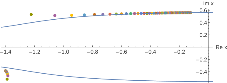
Figure 3: Single particle-hole pair excitations ($s=0$, $n_{c}=1$) according to equations (75). $T/J=0.1$, $h/h_{\ell}=2/3$, $\Delta=1.7$, $h_{\ell}/J=0.76$. Shown are particle-hole pairs for $n=1$ fixed and $m$ running from $-1$ to $-70$. The interaction with the particles slightly influences the hole position. The blue lines are the curves ${\rm Re\,}\varepsilon(x)=0$.

It is not difficult to solve the higher-level Bethe Ansatz equations (75) numerically. A simple example is shown in Figure 3. The example shows $70$ single particle-hole pairs ($s=0$, $n_{c}=1$). The quantum number $n$ of the hole is always $1$, the quantum number $m$ of the particle varies from $-1$ to $-70$. The particle and the hole in each pair are depicted by dots of the same colour.

For the calculation of correlation lengths below we need to calculate integrals over $\cal C$ that involve the auxiliary function $\mathfrak{a}$. Hence, we need $\mathfrak{a}$ on $\cal C$. Using the low-temperature picture obtained above, we obtain

$$\mathfrak{a}(x)=(-1)^{k}{\rm e}^{-\frac{\varepsilon(x)}{T}+\sum_{k=1}^{n_{c}}\varphi(x,y_{k})-\sum_{k=1}^{n_{c}+2s}\varphi(x,x_{k})}\bigl{(}1+{\cal O}(T^{\infty})\bigr{)}$$ (76)

for $x\in{\cal C}$.

We believe that at sufficiently low temperatures and finite magnetic field our self-consistent solutions to the nonlinear integral equations, described by the higher-level Bethe equations (75) and by the asymptotic auxiliary function (76), are complete. This means, in particular, that two particles or holes are not exponentially close to each other and not exponentially close to the real axis or to the line ${\rm Im\,}x=-\gamma$ for $T\rightarrow 0_{+}$, for all solutions leading to finite eigenvalue ratios in this limit. This belief is supported by numerical calculations for finite Trotter number (see Appendix A.3) and by the free Fermion picture that arises in the limit $T\rightarrow 0$. It leads us to the following

Conjecture.

For low temperatures at finite magnetic field every eigenstate of the quantum transfer matrix is parameterized by one of the solutions of the higher-level Bethe equations (75). This implies that all eigenstates can be interpreted in terms of particle-hole excitations.

In the limit $T\rightarrow 0_{+}$ at finite $s$ and $n_{c}$ the higher-level Bethe Ansatz equations (75) decouple, ${\rm i}\pi nT$ and ${\rm i}\pi mT$ turn into independent continuous variables, and the particles and holes become free parameters on the curves

$${\rm Re\,}\varepsilon(y)=0\,,\quad 0<{\rm Im\,}y<\gamma\,,$$ (77a)

$${\rm Re\,}\varepsilon(x)=0\,,\quad-\gamma<{\rm Im\,}x<0\,.$$ (77b)

These curves are shown in Figure 4. Clearly, the

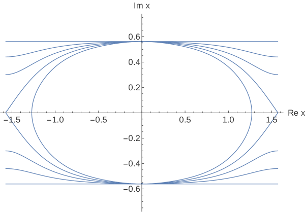
Figure 4: The curves ${\rm Re\,}\varepsilon(x)=0$ for various values of the magnetic field. Here $\Delta=1.7$, $h_{\ell}/J=0.76$. The values of the magnetic field decrease proceeding from the inner to the outer curve: $h/h_{\ell}=1.34,1,2/3,1/3,0$. The curves are closed for $h_{\ell}<h<h_{u}$. At the lower critical field $h=h_{\ell}$ they develop two cusps, and a gap opens for $0<h<h_{\ell}$.

massive regime is distinguished from the massless regime by the opening of a ‘band gap’ at the critical field $h_{\ell}$.

The case $s=n_{h}=0$ is special. In this case there are no higher-level Bethe Ansatz equations, and the auxiliary function is $\mathfrak{a}(x)=\pm{\rm e}^{-\epsilon(x)/T}$. The Bethe roots of the corresponding states are determined by $\mathfrak{a}(x)=\mp 1$ for $-\gamma<{\rm Im\,}x<0$, or

$$\epsilon(x)={\rm i}\pi nT\,,\quad-\gamma<{\rm Im\,}x<0\,,$$ (78)

where the $n$ are odd integers if $\mathfrak{a}(x)={\rm e}^{-\epsilon(x)/T}$ and even integers in the other case. Thus, the Bethe Ansatz equations decouple for $s=n_{c}=0$ (up to corrections of order $T^{\infty}$). We shall identify the corresponding states as the dominant state and a state which is degenerate up to corrections of the order $T^{\infty}$. An example of a Bethe root pattern of the dominant state is depicted in Figure 5.

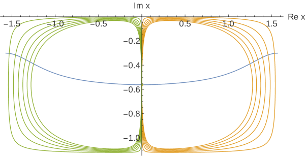
Figure 5: Bethe roots of the dominant state according to (78) depicted as the intersections of the curves ${\rm Re\,}\epsilon(x)=0$ and ${\rm Im\,}\epsilon(x)=n\pi T$ for $T/J=0.01$, $n=\pm 1,\pm 3,\dots,\pm 11$, $h/h_{\ell}=2/3$, $\Delta=1.7$, $h_{\ell}/J=0.76$. For growing $|n|$ the sequence of roots becomes more and more dense with an accumulation point at $-{\rm i}\gamma/2$ (intersection point of the curve ${\rm Re\,}\epsilon(x)=0$ with the imaginary axis).

With our low-temperature approximation (76) we can also check the consistency of the phase $k$ defined in (35). Let us consider the simple example $s=n_{c}=0$ and $k$ odd. Recall that we agreed to restrict the Bethe roots $x^{r}$ to $-\pi/2<{\rm Re\,}x^{r}\leq\pi/2$. Thus, the contours ${\cal C}_{\ell}$ and ${\cal C}_{r}$ should be slightly shifted (say, by a quantity of order $T^{2}$) on the line ${\rm Re\,}\varepsilon(x)=0$. This way one excludes the zero of $1+\mathfrak{a}$ which, for $k$ odd, has its real part very close (up to a correction of order $T^{\infty}$) to $-\pi/2$. At the same time one includes the $\pi$-shifted zero close to ${\cal C}_{r}$. With this convention for ${\cal C}_{\ell}$ we can now calculate the phase $k$. First of all,

$$\int_{{\cal C}_{\ell}}{\rm d}y\>\partial_{y}\ln(1+\mathfrak{a}(y))=\operatorname{PV}\int_{-\pi/2}^{-\pi/2-{\rm i}\gamma^{-}}{\rm d}y\>\partial_{y}\ln(1+\mathfrak{a}(y))-{\rm i}\pi\\ =\operatorname{Ln}(1+\mathfrak{a}(-\pi/2-{\rm i}\gamma^{-}))-\operatorname{Ln}(-1-\mathfrak{a}(-\pi/2))-{\rm i}\pi\,.$$ (79)

Here we took into account (76), which tells us that (up to a multiplicative correction of order $1+T^{\infty}$) $\mathfrak{a}$ is real on ${\cal C}_{\ell}$ with large negative values at $-\pi/2$ and small positive values at $-\pi/2-{\rm i}\gamma^{-}$. It further follows that the arguments of the logarithms on the right hand side of (79) have large positive real parts for small $T$. Inserting (79) into (35) and using that $\ln\mathfrak{a}(-\pi/2)=-\varepsilon(-\pi/2)/T-{\rm i}\pi k$ by (48), we obtain that $k=1$ (which is consistent with $k$ odd). Similar arguments apply for $s=n_{c}=0$ and $k$ even, in which case we find that $k=0$.

2.4 Root patterns and higher-level Bethe Ansatz equations for zero magnetic field

We would like to briefly comment on the case of vanishing magnetic field, $h=0$. We shall maintain our assumption that there are no exact strings. If $h=0$ the function $\mathfrak{a}^{(+)}$ becomes

$$\mathfrak{a}^{(+)}(x)=\biggl{[}\prod_{j=1}^{n_{h}}\frac{\sin(x-x_{j}^{h})}{\sin(x-x_{j}^{h}-{\rm i}\gamma)}\biggr{]}\\ \times\biggl{[}\prod_{j=1}^{n_{c}}\frac{\sin(x-x_{j}^{c}-{\rm i}\gamma)}{\sin(x-x_{j}^{c}+{\rm i}\gamma)}\biggr{]}\biggl{[}\prod_{j=1}^{n_{+}}\frac{\sin(x-x_{j}^{+}-{\rm i}\gamma)}{\sin(x-x_{j}^{+}+{\rm i}\gamma)}\biggr{]}\biggl{[}\prod_{j=1}^{n_{-}}\frac{\sin(x-x_{j}^{-}-2{\rm i}\gamma)}{\sin(x-x_{j}^{-})}\biggr{]}\,.$$ (80)

If there are no exact strings, then $\mathfrak{a}^{(0)}(x_{j}^{c})=0$, and the close roots and the far roots $x_{j}^{+}$ are determined by

$$\mathfrak{a}^{(+)}(x_{j}^{c})=-1\,,\quad\mathfrak{a}^{(+)}(x_{j}^{+})=-1\,.$$ (81)

This means that we cannot exclude the existence of far roots $x_{j}^{+}$ in this case, neither can we conclude as before that close roots form particle-hole strings. Similarly, far roots $x_{j}^{-}$ may exist as well and satisfy

$$\mathfrak{a}^{(-)}(x_{j}^{-})=-1\,,$$ (82)

where $\mathfrak{a}^{(-)}(x)=\mathfrak{a}^{(+)}(x+{\rm i}\gamma)$.

Holes must satisfy the equation

$$\mathfrak{a}^{(0)}(x_{j}^{h})=-1\,,$$ (83)

where

$$\mathfrak{a}^{(0)}(x)=(-1)^{k}A(x){\rm e}^{-\frac{\varepsilon(x)}{T}}\biggl{[}\prod_{j=1}^{n_{h}}\frac{\sin(x-x_{j}^{h}+{\rm i}\gamma)}{\sin(x-x_{j}^{h}-{\rm i}\gamma)}\biggr{]}\\ \times\biggl{[}\prod_{j=1}^{n_{c}}\frac{\sin(x-x_{j}^{c})}{\sin(x-x_{j}^{c}+{\rm i}\gamma)}\biggr{]}\biggl{[}\prod_{j=1}^{n_{-}}\frac{\sin(x-x_{j}^{-}-{\rm i}\gamma)}{\sin(x-x_{j}^{-})}\biggr{]}\biggl{[}\prod_{j=1}^{n_{+}}\frac{\sin(x-x_{j}^{+})}{\sin(x-x_{j}^{+}+{\rm i}\gamma)}\biggr{]}\,.$$ (84)

Clearly holes may exist close to the line ${\rm Im\,}x=-\gamma/2$, where ${\rm Re\,}\varepsilon(x)=0$. Let us discuss the situation away from this line. Suppose that ${\rm Re\,}\varepsilon(x_{j}^{h})<0$. Then, for (83) to hold, there must be an $x_{k}^{-}$ such that $x_{j}^{h}-x_{k}^{-}-{\rm i}\gamma\rightarrow 0$ as $T\rightarrow 0_{+}$. This implies that $\mathfrak{a}^{(-)}(x_{k}^{-})\rightarrow 0$ which cannot be. If, on the other hand, ${\rm Re\,}\varepsilon(x_{j}^{h})>0$, then (83) can only hold if there is an $x_{k}^{c}$ such that $x_{j}^{h}-x_{k}^{c}+{\rm i}\gamma\rightarrow 0$ as $T\rightarrow 0_{+}$. But this implies that $1/\mathfrak{a}^{(+)}(x_{k}^{c})\rightarrow 0$ which is impossible.

Thus, holes can exist only close to the line ${\rm Im\,}x=-\gamma/2$. As $T\rightarrow 0_{+}$ they densely fill the line segment $-{\rm i}\gamma/2+[-\pi/2,\pi/2]$. This means that the holes become free parameters as $T\rightarrow 0_{+}$, whereas close roots and far roots remain constrained by the higher-level Bethe Ansatz equations (81), (82). This is in stark contrast to the case of finite magnetic field where both, particle and hole parameters, become free for $T\rightarrow 0_{+}$.

Note that the higher-level Bethe Ansatz equations become uniform if we perform the following change of variables,

$$\{\chi_{j}\}_{j=1}^{n_{\chi}}=\{x_{j}^{c}-{\rm i}\gamma/2\}_{j=1}^{n_{c}}\cup\{x_{j}^{+}-{\rm i}\gamma/2\}_{j=1}^{n_{+}}\cup\{x_{j}^{-}+{\rm i}\gamma/2\}_{j=1}^{n_{-}}\,.$$ (85)

With these variables the higher-level Bethe Ansatz equations (81), (82) turn into

$$-1=\biggl{[}\prod_{k=1}^{n_{h}}\frac{\sin(\chi_{j}-x_{k}^{h}+{\rm i}\gamma/2)}{\sin(\chi_{j}-x_{k}^{h}-{\rm i}\gamma/2)}\biggr{]}\biggl{[}\prod_{j=1}^{n_{\chi}}\frac{\sin(\chi_{j}-\chi_{k}-{\rm i}\gamma)}{\sin(\chi_{j}-\chi_{k}+{\rm i}\gamma)}\biggr{]}\,,$$ (86)

$j=1,\dots,n_{\chi}$, where

$$n_{\chi}=n_{c}+n_{f}=\frac{n_{h}}{2}-s\,.$$ (87)

Equations (86) are of the same form as the higher-level Bethe Ansatz equations for the ordinary transfer matrix in the antiferromagnetic massive regime [2, 28] (see also our recent discussion in [7]).

2.5 Correlation lengths at low temperatures and finite magnetic field

We now turn back to finite magnetic field $h>0$. Starting from equation (10) which expresses the quantum transfer matrix eigenvalues in terms of Bethe roots and employing a similar reasoning as in the derivation of the nonlinear integral equations in Section 2.1 we obtain the representation

$$\Lambda(x)=\biggl{(}\frac{\cos({\rm i}\gamma/2+x)}{\cos({\rm i}\gamma/2-x)}\biggr{)}^{d}\biggl{[}\prod_{j=1}^{n_{h}}\frac{\sin(x-x_{j}^{h}-{\rm i}\gamma/2)}{\sin(x-x_{j}^{h}+{\rm i}\gamma/2)}\biggr{]}\biggl{[}\prod_{j=1}^{n_{c}}\frac{\sin(x-x_{j}^{c}+3{\rm i}\gamma/2)}{\sin(x-x_{j}^{c}-{\rm i}\gamma/2)}\biggr{]}\\ \times\exp\biggl{\{}\frac{h}{2T}-\int_{\cal C}{\rm d}y\>K(x-y|\gamma/2)\ln_{\cal C}(1+\mathfrak{a}(y))\biggr{\}}$$ (88)

valid for $-\gamma/2<{\rm Im\,}x<\gamma/2$. This is the general expression for $\Lambda$, still valid for any temperature and magnetic field $h\geq 0$, in the case that there are no far roots. If far roots are present, an additional factor of

$$\prod_{j=1}^{n_{f}}\frac{\sin(x-x_{j}^{f}+{\rm i}\gamma/2)}{\sin(x-x_{j}^{f}-{\rm i}\gamma/2)}$$ (89)

appears on the right hand side of (88).

In the low-$T$ limit at $h>0$ there are no far roots, and the close roots form strings with holes. Using (71) and (2.3) as well as the facts that $\mathfrak{a}^{-1}(x)={\cal O}(T^{\infty})$ for $x\in{\cal C}_{+}$ and $\mathfrak{a}(x)={\cal O}(T^{\infty})$ for $x\in{\cal C}_{-}$ in (88) we obtain

$$\Lambda(x)=\biggl{(}\frac{\cos({\rm i}\gamma/2+x)}{\cos({\rm i}\gamma/2-x)}\biggr{)}^{d}\biggl{[}\prod_{j=1}^{n_{c}+2s}\frac{\sin(x-x_{j}-{\rm i}\gamma/2)}{\sin(x-x_{j}+{\rm i}\gamma/2)}\biggr{]}\biggl{[}\prod_{j=1}^{n_{c}}\frac{\sin(x-y_{j}+{\rm i}\gamma/2)}{\sin(x-y_{j}-{\rm i}\gamma/2)}\biggr{]}\\ \times\exp\biggl{\{}\frac{h}{2T}+\int_{-\pi/2}^{\pi/2}{\rm d}y\>K(x-y|\gamma/2)\ln\mathfrak{a}(y)\biggr{\}}\bigl{(}1+{\cal O}(T^{\infty})\bigr{)}\,.$$ (90)

We shall denote the eigenvalue with $n_{c}=s=k=0$ by $\Lambda_{0}(x)$. This eigenvalue has the representation

$$\Lambda_{0}(x)=\exp\biggl{\{}\frac{h}{2T}-\frac{1}{T}\int_{-\pi/2}^{\pi/2}{\rm d}y\>K(x-y|\gamma/2)\varepsilon(y)\biggr{\}}\bigl{(}1+{\cal O}(T^{\infty})\bigr{)}\,.$$ (91)

We shall argue below that this eigenvalue is the dominant eigenvalue. We are interested in the ratio $\rho(0|\alpha)$ of the eigenvalue of a twisted excited state (with $h\rightarrow h^{\prime}=h-2\alpha\gamma T$, $\alpha$ twist parameter) and the untwisted dominant state. Using (90) we find that, up to corrections of the order ${\cal O}(T^{\infty})$,

$$\rho(0|\alpha)=(-1)^{k}\biggl{[}\prod_{j=1}^{n_{c}+2s}\frac{\sin(x_{j}+{\rm i}\gamma/2)}{\sin(x_{j}-{\rm i}\gamma/2)}\biggr{]}\biggl{[}\prod_{j=1}^{n_{c}}\frac{\sin(y_{j}-{\rm i}\gamma/2)}{\sin(y_{j}+{\rm i}\gamma/2)}\biggr{]}\\ \times\exp\biggl{\{}\int_{-\pi/2}^{\pi/2}{\rm d}x\>K(x|\gamma/2)\biggl{[}\sum_{k=1}^{n_{c}}\varphi(x,y_{k})-\sum_{k=1}^{n_{c}+2s}\varphi(x,x_{k})\biggr{]}\biggr{\}}\,.$$ (92)

Note that the dependence on the twist parameter $\alpha$ has been entirely absorbed by the roots $x_{j}$, $y_{j}$.

Equation (92) can be further simplified. For this purpose we recall (see e.g. [7]) that the momentum $p$ satisfies the linear integral equation

$$p(x)=\frac{p_{0}(x)}{2\pi}-\frac{\theta(x-\pi/2)}{4\pi{\rm i}}-\int_{-\pi/2}^{\pi/2}{\rm d}y\>K(x-y)p(y)\,,$$ (93)

where $p_{0}(x)=-{\rm i}\theta(x|\gamma/2)$ (for an explicit form of the solution of the integral equation see Appendix A.1). Combining (93) with (42b) we obtain

$$p(x)+\frac{\varphi(x,\pi/2)}{2\pi{\rm i}}=\frac{p_{0}(x)}{2\pi}-\int_{-\pi/2}^{\pi/2}{\rm d}y\>K(x-y)\biggl{(}p(y)+\frac{\varphi(y,\pi/2)}{2\pi{\rm i}}\biggr{)}\,.$$ (94)

Then, applying partial integration and the dressed function trick to the integral in (92), we find that

$$\int_{-\pi/2}^{\pi/2}{\rm d}x\>K(x|\gamma/2)\varphi(x,z)={\rm i}\pi+2\pi{\rm i}p(z)-{\rm i}p_{0}(z)\,.$$ (95)

Using the latter equation in (92) we arrive at the main result of this work which is a formula for the eigenvalue ratios $\rho(0|\alpha)$ in the antiferromagnetic massive regime at finite magnetic field in terms of the particle and hole roots $y_{j}$, $x_{k}$ determined by the higher-level Bethe Ansatz equations (75):

$$\rho(0|\alpha) =(-1)^{k}\exp\biggl{\{}2\pi{\rm i}\Bigl{[}\sum_{j=1}^{n_{c}}p(y_{j})-\sum_{j=1}^{n_{c}+2s}p(x_{j})\Bigr{]}\biggr{\}}$$

$$=(-1)^{k}\biggl{[}\prod_{j=1}^{n_{c}}\frac{\vartheta_{1}(y_{j}-{\rm i}\gamma/2|q^{2})}{\vartheta_{4}(y_{j}-{\rm i}\gamma/2|q^{2})}\biggr{]}\biggl{[}\prod_{j=1}^{n_{c}+2s}\frac{\vartheta_{4}(x_{j}-{\rm i}\gamma/2|q^{2})}{\vartheta_{1}(x_{j}-{\rm i}\gamma/2|q^{2})}\biggr{]}\,,$$ (96)

this being valid up to multiplicative corrections of the order $\bigl{(}1+{\cal O}(T^{\infty})\bigr{)}$. Remarkably, the second representation of the eigenvalue ratios in (2.5) is completely explicit in terms of the particle and hole parameters.

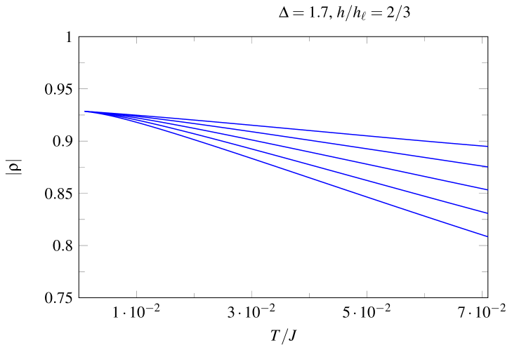
Figure 6: The behaviour of $|\rho|$ as a function of temperature for one hole and one particle. The particle and hole roots are obtained from the higher-level Bethe Ansatz equations (75) for $n=1$, $m=-1,-3,-5,-7,-9$ (from top to bottom) and inserted into (2.5). The parameters are chosen as $h/h_{\ell}=2/3$, $\Delta=1.7$, $h_{\ell}/J=0.76$, $\alpha=0$.

Setting $s=n_{c}=0$ we obtain $\rho(0|\alpha)=\pm 1$. For all other states not both, $s$ and $n_{c}$, are zero. Hence, using (A.3) in (2.5) we conclude that $|\rho(0|\alpha)|<1$ for all other states. Then, referring to our conjecture of the previous subsection, one of the states with $s=n_{c}=0$ must be the dominant state (or the dominant state is two-fold degenerate). It is possible to see, by solving the nonlinear integral equation (25) numerically, that the dominant state corresponds to $k=0$ or, equivalently, to $\mathfrak{a}(x)={\rm e}^{-\epsilon(x)/T}$ and $\Lambda_{0}(x)$, equation (91), at low temperatures. The gap between the dominant state and the almost degenerate state is of the order $T^{\infty}$.

2.6 Discussion

The behaviour of the correlation lengths as functions of temperature can be extracted from equations (75) and (2.5). An example is shown in Figure 6. In this example $s=0$ and $n_{c}=1$ as in Figure 3. States with these quantum numbers appear in the form factor expansion of the longitudinal two-point functions $\langle\sigma_{1}^{z}\sigma_{n}^{z}\rangle$. The figure shows $|\rho|$ where $\rho=\rho(0,0)$. The corresponding correlation lengths are $\xi=-1/\ln|\rho|$. The excitations leading to the eigenvalue ratios shown in the figure have quantum numbers $n=1$ and $m=-1,-3,-5,-7,-9$ from top to bottom. The top curve corresponds to the leading correlation length. As expected $|\rho|$ and hence the corresponding correlation length $\xi$ decreases with increasing temperature. For $T\rightarrow 0_{+}$ infinitely many correlation lengths degenerate and the spectrum becomes dense. Thus, a summation (or integration) over these infinitely many contributions is necessary for the calculation of the two-point functions at zero temperature. This will result in correlation lengths of the zero-temperature correlation functions which are different from the values of $\xi$ for $T\rightarrow 0_{+}$. In other words, our above formulae determine the physical correlation lengths only for small but finite temperatures.

Nevertheless it is interesting to calculate the value of $|\rho|$ for $T\rightarrow 0_{+}$. It can be obtained from the energy-momentum relation (A.11). Denoting the particle position by $y$ and the hole position by $x$ we have, according to (2.5), $|\rho|=|{\rm e}^{2\pi{\rm i}p(y)}||{\rm e}^{-2\pi{\rm i}p(x)}|$, where $x$ and $y$ are determined by the higher-level Bethe Ansatz equations (75). For $T\rightarrow 0_{+}$ they simplify to $\varepsilon(x)=\varepsilon(y)=0$. For this reason we can determine $|\rho|$ from (A.11) by setting the left hand side equal to zero and solving for ${\rm e}^{2\pi{\rm i}p}$. Equations (A.3) allow us to detect which solution of the quadratic equation belongs to the particle and which one to the hole. After an elementary calculation we end up with

$$|\rho|=\Biggl{[}\sqrt{\frac{1}{k^{2}}-\biggl{(}\frac{1}{k^{2}}-1\biggr{)}\biggl{(}\frac{h}{h_{\ell}}\biggr{)}^{2}}-\sqrt{\biggl{(}\frac{1}{k^{2}}-1\biggr{)}\biggl{(}1-\biggl{(}\frac{h}{h_{\ell}}\biggr{)}^{2}\biggr{)}}\Biggr{]}^{2}$$ (97)

which reduces to a well-known result [11] for $h=0$. The monotonic behaviour as a function of $h$ with maximum $|\rho|=1$ at $h=h_{\ell}$ corresponds to the linear decrease of the mass gap (see (A.11)) as a function of the magnetic field. At $h=h_{\ell}$ the mass gap closes, and the correlation length diverges in accordance with our intuition.

3 Conclusions

We have considered the spectrum of the quantum transfer matrix of the XXZ chain in the antiferromagnetic massive regime and have worked out in detail the case of low temperatures at finite magnetic field $0<h<h_{\ell}$.

The nonlinear integral equation for a suitable auxiliary function was cast into a form such that the low-temperature limit could be immediately taken. A careful analysis of the resultant simplified equations in the entire complex rapidity plane showed that roots away from the distribution center (far roots) cannot exist. More importantly, our analysis suggests that at low temperatures all excitations can be classified as particle-hole excitations. The ratios of the eigenvalues to the dominant eigenvalue of the quantum transfer matrix turned out to be explicit functions of the particle and hole parameters which satisfy a set of higher-level Bethe Ansatz equations at small finite $T$. These parameters become free on two curves in the complex plane as $T\rightarrow 0_{+}$. We conjecture that for finite magnetic field at low temperatures all eigenvalue ratios are of this form.

Our conjecture implies that only particle-hole excitations have to be taken into account in the calculation of correlation functions by means of a form factor expansion. This is rather reminiscent of previous studies of the massless regime [5, 6]. Still, there are two differences. The configurations of particle-hole pairs differ in that, in the massive case considered here, another hole is rigidly attached in a string-like manner to every particle. Yet, this may be seen as an artefact related to our choice of the integration contour. More importantly, the summation of all particle-hole excitations may have a different meaning in the massive and in the massless case. In the massless case it is based on a ‘critical form factor summation formula’. In the context of the analysis of the large-distance asymptotics of correlation functions this formula first appeared in [19], where it was applied to the interacting Bose gas at finite temperature. A proof and an analysis of the ground state two-point functions of the XXZ chain in the critical regime were supplied in [12], and an analysis of the finite temperature case followed in [5, 6]. In those works it was argued that a restriction of the summation to the gapless particle-hole excitations would give the low-energy long-wave length contribution to the two-point functions and hence their large-distance asymptotics. By way of contrast, we expect that a summation over all particle-hole contributions in the massive antiferromagnetic regime will give the full two-point functions at any distance in a similar way as in the zero temperature case [10, 7].

We believe that we are now in the position to study two-point correlation functions at low temperatures in the antiferromagnetic massive regime. We hope to report first progress in near future.
Acknowledgment. The authors are grateful to A. Klümper for helpful discussions and for his interest in this work. MD and FG acknowledge financial support by the Volkswagen Foundation and by the Deutsche Forschungsgemeinschaft under grant number Go 825/7-1. KKK is supported by the CNRS. His work has been partly financed by a Burgundy region PARI 2013-2014 FABER grant ‘Structures et asymptotiques d’intégrales multiples’. KKK also enjoys support from the ANR ‘DIADEMS’ SIMI 1 2010-BLAN-0120-02. JS is supported by a JSPS Grant-in-Aid for Scientific Research (C) No. 15K05208.

Appendix A: Basic functions

In this appendix we gather explicit representations of the basic functions appearing in the low-temperature analysis of the antiferromagnetic massive regime. These are the momentum, the dressed energy and the dressed phase. Fourier series are the starting point for the derivation of the various representations and properties of these functions. The Fourier coefficients can be directly obtained from the respective linear integral equations by means of the convolution theorem. Derivations of most of the formulae can be found in the appendices of [7].

A.1 Momentum

Fourier series representation:

$$p(x)=\frac{1}{4}+\frac{x}{2\pi}+\sum_{n=1}^{\infty}\frac{1}{n\pi}\;\frac{\sin(2nx)}{q^{n}+q^{-n}}\,.$$ (A.1)

Representation in terms of Jacobi-theta functions:

$$p(x)=\frac{1}{4}+\frac{x}{2\pi}+\frac{1}{2\pi{\rm i}}\ln\biggl{(}\frac{\vartheta_{4}(x+{\rm i}\gamma/2|q^{2})}{\vartheta_{4}(x-{\rm i}\gamma/2|q^{2})}\biggr{)}\,.$$ (A.2)

Behaviour above and below the real axis:

$$\begin{split}&{\rm Re\,}\bigl{[}2\pi{\rm i}p(x)\bigr{]}<0\quad\text{for}\ 0<{\rm Im\,}x<\gamma\,,\\[2.15277pt] &{\rm Re\,}\bigl{[}2\pi{\rm i}p(x)\bigr{]}>0\quad\text{for}\ -\gamma<{\rm Im\,}x<0\,.\end{split}$$ (A.3)

From (A.2) we obtain the formula

$$\cos\bigl{(}2\pi p(x)\bigr{)}=-\operatorname{sn}\biggl{(}\frac{2Kx}{\pi}\bigg{|}k\biggr{)}\,,$$ (A.4)

where now $k$ is the elliptic modulus, $K=K(k)$ is the complete elliptic integral of the first kind and $K^{\prime}=K(\sqrt{1-k^{2}})$. The elliptic modulus parameterizes $\gamma$ as $\gamma=\pi K^{\prime}/K$. The function $\operatorname{sn}$ is the Jacobi-elliptic $\operatorname{sn}$-function.

A.2 Dressed energy

The dressed energy is the solution of the linear integral equation (40). It has the following series representations.

Fourier series representation:

$$\varepsilon(x)=\frac{h}{2}-4J\operatorname{sh}(\gamma)\sum_{n\in{\mathbb{Z}}}\frac{{\rm e}^{2{\rm i}nx}}{q^{n}+q^{-n}}\,.$$ (A.5)

Poisson-resummed series:

$$\varepsilon(x)=\frac{h}{2}-\frac{2\pi J\operatorname{sh}(\gamma)}{\gamma}\sum_{n\in{\mathbb{Z}}}\frac{1}{\operatorname{ch}\bigl{(}\frac{\pi}{\gamma}(x-n\pi)\bigr{)}}\,.$$ (A.6)

Equation (A.6) defines the dressed energy as a meromorphic function in the complex plane. We see from this formula that $\varepsilon$ is double periodic. It can be expressed it in terms of the Jacobi-dn function.

$$\varepsilon(x)=\frac{h}{2}-\frac{4JK\operatorname{sh}(\gamma)}{\pi}\operatorname{dn}\biggl{(}\frac{2Kx}{\pi}\bigg{|}k\biggr{)}$$ (A.7)

From (A.6) we can also readily read off the functional equation

$$\varepsilon(x)+\varepsilon(x+{\rm i}\gamma)=h$$ (A.8)

and the periodicity

$$\varepsilon(x+\pi)=\varepsilon(x)\,.$$ (A.9)

Let us recall that the lower critical field $h_{\ell}$ is defined by the condition $\varepsilon(\pi/2)~{}=~{}0$, implying that

$$h_{\ell}=\frac{8JK\operatorname{sh}(\pi K^{\prime}/K)}{\pi}\operatorname{dn}(K|k)\,.$$ (A.10)

One can show that $\varepsilon$ is even and monotonously increasing for $0<x<\pi/2$. Hence, $0<h<h_{\ell}$ implies that $\varepsilon(x)<0$ for all $x\in[-\pi/2,\pi/2]$, and it follows that ${\rm Re\,}\bigl{(}-T\ln(\mathfrak{a})\bigr{)}$ is positive on ${\cal C}_{+}$ if $T$ is small enough. Then (A.6) implies that $\varepsilon(x+{\rm i}\gamma)=h-\varepsilon(x)>0$, whence ${\rm Re\,}\bigl{(}-T\ln(\mathfrak{a})\bigr{)}$ is negative on ${\cal C}_{-}$ if only $T$ is small enough. These were the conditions from which we started our low-temperature analysis. They are self-consistently satisfied if $0\leq h<h_{\ell}$, i.e. if we are in the antiferromagnetic massive regime.

Reinserting (A.10) into (A.7) and using (A.4) we obtain the energy-momentum relation

$$\varepsilon(p)=\frac{h}{2}-\frac{h_{\ell}}{2}\sqrt{\frac{1-k^{2}\cos^{2}(2\pi p)}{1-k^{2}}}\,.$$ (A.11)

A.3 Dressed phase

Fourier series representation of $\varphi(*,z)$ for $|{\rm Im\,}z|<\gamma$:

$$\varphi(x,z)={\rm i}(\pi/2+x-z)+\sum_{n=1}^{\infty}\frac{2{\rm i}}{n}\;\frac{\sin\bigl{(}2n(x-z)\bigr{)}}{1+q^{-2n}}\,.$$ (A.12)

This series can be resummed and expressed in terms of $q$-$\Gamma$ functions:

$$\varphi(x_{1},x_{2})={\rm i}\Bigl{(}\frac{\pi}{2}+x_{12}\Bigr{)}+\ln\Biggl{\{}\frac{\Gamma_{q^{4}}\bigl{(}1+\frac{{\rm i}x_{12}}{2\gamma}\bigr{)}\Gamma_{q^{4}}\bigl{(}\frac{1}{2}-\frac{{\rm i}x_{12}}{2\gamma}\bigr{)}}{\Gamma_{q^{4}}\bigl{(}1-\frac{{\rm i}x_{12}}{2\gamma}\bigr{)}\Gamma_{q^{4}}\bigl{(}\frac{1}{2}+\frac{{\rm i}x_{12}}{2\gamma}\bigr{)}}\Biggr{\}}\,,$$ (A.13)

where $x_{12}=x_{1}-x_{2}$ and $|{\rm Im\,}x_{2}|<\gamma$. Here $\Gamma_{q}$ is defined by the infinite product

$$\Gamma_{q}(x)=(1-q)^{1-x}\prod_{n=1}^{\infty}\frac{1-q^{n}}{1-q^{n+x-1}}\,.$$ (A.14)

Let us also recall the definition of a $q$-number

$$[x]_{q}=\frac{1-q^{x}}{1-q}\,.$$ (A.15)

Using $q$-numbers the fundamental recursion relation of the $q$-$\Gamma$ functions becomes

$$\Gamma_{q}(x+1)=[x]_{q}\Gamma_{q}(x)\,,\quad\Gamma_{q}(1)=1\,.$$ (A.16)

It implies that the dressed phase obeys the functional equation

$${\rm e}^{\varphi(x_{1},x_{2})+\varphi(x_{1}+{\rm i}\gamma,x_{2})}=\frac{\sin(x_{1}-x_{2})}{\sin(x_{1}-x_{2}+{\rm i}\gamma)}\,.$$ (A.17)

We further have the quasi-periodicity

$$\varphi(x+\pi,z)=\varphi(x,z)+{\rm i}\pi\,.$$ (A.18)

For $|{\rm Im\,}z|>\gamma$ we have the explicit representation

$${\rm e}^{\varphi(x,z)}=\begin{cases}\displaystyle\frac{\sin(x-z)}{\sin(x-z+{\rm i}\gamma)}&\text{if ${\rm Im\,}z>\gamma$}\\[17.22217pt] \displaystyle\frac{\sin(x-z-{\rm i}\gamma)}{\sin(x-z)}&\text{if ${\rm Im\,}z<-\gamma$}\,.\end{cases}$$ (A.19)

Appendix B: Numerical study

In this appendix we supply numerical results for finite Trotter numbers in order to support claims made in the main text.

It is not hard to solve numerically the Bethe Ansatz equations for low-lying excited states of the ordinary transfer matrix of the six-vertex model which determine the spectrum of the XXZ Hamiltonian and its correlation functions at $T=0$. In this case the magnetic field $h$ does not change the location of the roots: it merely changes the energy eigenvalues through the Zeeman term in the Hamiltonian. The situation is completely different in the finite temperature case: the Bethe Ansatz equations depend on both $h$ and $T$. The root distributions then exhibit diverse behavior with changes in $h$ or in $T$, depending on the states under consideration. There occur, moreover, crossings of energy levels. These prevent us from drawing a simple conclusion about the general root patterns pertaining to the relevant eigenstates.

We thus do not trace Bethe roots for specially chosen (low-lying) states, but study all possible configurations of the Bethe roots for a fixed Trotter number $N$. The actual procedure combines the numerical diagonalization of the quantum transfer matrix with symbolic manipulations on Baxter’s TQ relation [4] as proposed for the first time in [1]. This, of course, restricts the possible values of $N$ to small numbers: typically we shall set $N=8$ or 10, while the logic of the quantum transfer matrix formalism would rather require $N$ infinity. At least the parameter $|\beta/N|$ must be chosen small. We shall impose the condition $|\beta/N|<1/2$ which implies that very low values of $T$ cannot be reached. Nevertheless, the full list of Bethe-root distributions reveals a simple characterization of the relevant eigenstates for a non-vanishing magnetic field.

B.1 Reduction of strings

The existence of longer strings implies the existence of far roots. Below we argue that the dominant contributions to the spectrum of correlation lengths do not include longer strings in the low temperature limit at non-zero magnetic fields.

We fix the value of $h$. For sufficiently high temperatures longer strings do exist. With decrease in temperature, roots change their locations continuously except at discrete values, $T_{m}=\frac{h}{2m\gamma}$, $m\in\mathbb{N}$. By approaching $T_{m}$ from above, some of the roots go to infinity (${\rm Im\,}x_{j}\rightarrow+\infty$). We call them diverging roots. To be precise, led by numerical investigations, we arrive at the following

Conjecture 1.

Consider eigenstates in the sector with spin $s$, or equivalently $M=\frac{N}{2}-s$ Bethe roots, at $T\sim T_{m}$. If $s+1\leq m\leq\frac{N}{2}$, there are ${N\choose N/2-m}$ eigenstates (out of totally ${N\choose M}$ states in the sector) with $m-s$ diverging roots.

Case studies for $N=4,\dots,10$ with various choices of parameters confirm that there is no exception to the above rule. There is, however, a subtle point. Due to the condition $|\beta/N|<1/2$, $h$ can not be too small in order to reach the singular values of $T$. Some of the trials leading to the above conjecture were thus performed outside of the range $h<h_{\ell}$. As far as we have observed, the massive phase and the massless phase share the same divergent behavior. Thus, we temporarily neglect the condition $h<h_{\ell}$. After crossing a singular value $T_{m}$ of $T$, the diverging roots come back to finite locations. We observe that their positions are different from those at $T$ slightly above $T_{m}$. This abrupt change of locations at singular values of $T$ is the main mechanism for the reduction of strings. We demonstrate this with the example of a 4-string solution, $N=8,s=0,\gamma=1$. In order to achieve low $T$ we take relatively large magnetic field, $h=10$. The snapshots of Bethe roots with decrease in $T$ are depicted in Figure 7. Clearly, the string becomes shorter every time $T$ crosses a singular value.

Figure 7: The fate of Bethe roots composing a 4 string at sufficiently high $T$. We fix $h=10$ and $\gamma=1$. $T=10,4,2$ (upper row), $T=1.5,1.1$ (lower row) from the left to right.

The states with diverging roots involve strings at sufficiently high temperatures. We have no explanation why the converse should be true, but it seems empirically the case. Let $\Lambda_{j}$ be the $j$th eigenvalue of the quantum transfer matrix. We arrange the $|\Lambda_{j}|$ in decreasing order and refer to them as ‘energy levels’. We then count the number of states with diverging roots in every 10 consecutive ‘energy levels’ at $T$ slightly above $T_{m}$. An example for $N=8,\gamma=3,h=16$ and $s=0$ is depicted in Figure 8. The sector contains 70 states. Thus, we divide them in 7 portions. The horizontal axis represents the ‘energy level’. The height of the leftmost bin represents the number of states with diverging roots among the first 10 ‘energy levels’, and so on. The figure manifestly shows that, as temperature goes down, states with diverging roots become higher and higher excited states. This suggests that, after sufficiently many crossings of singular values $T_{m}$, even if there still remain states containing strings, these should be highly excited. We thus conclude that they do not significantly contribute to correlations at finite temperatures.

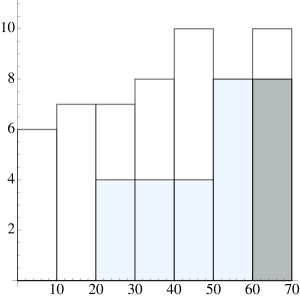
Figure 8: The white, light blue and grey bins represent the distributions of diverging-root states slightly above $T_{1}=h/2\gamma,T_{2}=h/4\gamma$ and $T_{3}=h/6\gamma$, respectively. The heights ($=8$) of the rightmost bins are identical for $T_{2}$ and $T_{3}$.

B.2 Dominant contributions

We proceed further and claim that free holes and particle-hole pairs provide a complete description of the dominant excitations. Let us illustrate this with an example, $N=\nolinebreak 8$, $h=3.7$, $\gamma=2$ and $s=0$. Consider the case $T=2$. We present the three Bethe-root configurations which correspond to the first three ‘energy levels’ in Figure 9. We omit configurations with complex conjugate eigenvalues, which are obtained by a simple reflection. The figure illustrates the high-temperature regime, $T>h/2\gamma$. One observes 2-string states but no particle-hole bound pairs. Figure 10 shows the three configurations corresponding to the last three ‘energy levels’. They are all characterized by 4-strings, and the holes are more densely distributed on the line ${\rm Im\,}x=-\gamma/2$.

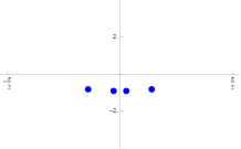
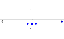
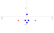
Figure 9: ‘Top 3’ configurations at $T=2$. Blue circles represent Bethe roots while red triangles are holes.

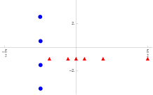
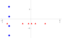
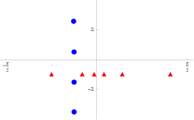
Figure 10: ‘Worst 3’ configurations at $T=2$.

Next, we consider the case $T=0.46<h/4\gamma$, which is reached after passing two critical temperatures. The three Bethe root configurations corresponding to the three eigenvalues of largest modulus are given in Figure 11. We do not observe strings anymore. Instead, we observe a particle-hole pair in each state (except for the dominant one).

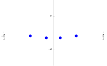
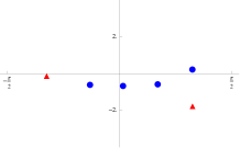
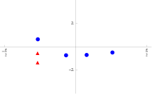
Figure 11: ‘Top 3’ configurations at $T=0.46$.

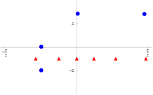
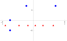
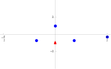
Figure 12: ‘Worst 3’ configurations at $T=0.46$.

Figure 12 shows the last three configurations at the same temperature. One still observes 2 strings, which may be remains of 4 strings, but no particle-hole pairs.

The highly excited states do not affect the physical quantities. They are physically irrelevant. All particle-hole pair excitations, on the other hand, are low-lying and therefore physical. To turn this into a quantitative argument we introduce a quantity

$$\mathfrak{r}=\frac{\sum_{\text{sum over particle-hole excitations}}|\Lambda_{j}|}{\sum_{\text{sum over all but the ground state}}|\Lambda_{j}|}\,.$$ (B.1)

Clearly, $\mathfrak{r}$ measures the relative importance of the particle-hole excitations. There is, of course, a certain ambiguity in identifying the particle-hole excitations. The explicit value of $\mathfrak{r}$ depends on the identification criterion. Its qualitative temperature behaviour, however, seems to be independent of the choice. We tabulate the values of $\mathfrak{r}$ and the number of pairs $n_{\text{pair}}$ in Table 1.

T	$0.9$	$0.8$	$0.7$	$0.6$	$0.5$
$n_{\text{pair}}$	$0$	$4$	$10$	$20$	$29$
$\mathfrak{r}$	$0$	$0.167$	$0.335$	$0.849$	$0.917$

Table 1: The numbers of the particle-hole pairs and values of $\mathfrak{r}$ at various temperatures for $N=8,\gamma=2,h=3.7$ and $s=0$.

Strictly speaking there are four states with accidental pairs at $T=0.9$. We checked that they correspond to a situation in which the center of a 3 string and a hole come very close to each other, hence, we neglect them. Even for $h=0$ there are such accidental pairs. We checked that their contribution is independent of $T$ and very minor (less than 1%).

To understand which levels contribute to $\mathfrak{r}$, we counted again the number of states with particle-hole pairs in every 10 consecutive ‘energy levels’. The corresponding histogram for $T=0.5$ is presented in Figure 13. Table 1 and the histogram clearly show that the particle-hole pairs become the dominant excitations when the temperature decreases at fixed finite $h$ in the $s=0$ sector.

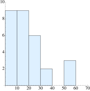
Figure 13: The vertical axis represents the number of states with pairs in every 10 consecutive ‘energy levels’. In the first bin, only the ground state is missing, while the 20th level is missing in the 2nd bin and so on.

Next consider sectors with $s\neq 0$. We chose $\gamma=3$, fixed $h=16$, and calculated the values of $\mathfrak{r}$ in several sectors for $N=8,10$ and $N=12$. The results are summarized in Table 2. For this choice of the parameters $\mathfrak{r}$ is equal to unity in the $s=0$ sector, that is, any but the ground state carries particle-hole pairs. The number of particle-hole pairs and their contribution to $\mathfrak{r}$ decrease in the higher-$s$ sectors. Thus, particle-hole pairs become less important. Instead, we find that low-lying excitations in the $s\neq 0$ sectors are characterized by free holes. Take $N=8$ and $s=1$ as an example. The first 10 ‘energy levels’ do not include particle-hole pairs, resulting in a small $\mathfrak{r}$. We find numerically that there exist 5 available positions for roots and holes near the real axis. In the present case, three roots and two holes must be allocated there. This amounts to 10 possible configurations, and we checked that they generate nothing but the first 10 states. Three examples are shown in Figure 14. Similarly we find that also the most important contributions in other $s\neq 0$ sectors come from free holes.

	$N=8$		$N=10$		$N=12$
s	$\mathfrak{r}$	$n_{\text{pairs}}/n_{\text{total}}$	$\mathfrak{r}$	$n_{\text{pairs}}/n_{\text{total}}$	$\mathfrak{r}$	$n_{\text{pairs}}/n_{\text{total}}$
1	0.378	46/56	0.351	178/210	*	*
2	0.115	12/28	0.035	46/120	0	0/66
3	0.05	1/8	0	0/45	0	0/220

Table 2: The values of $\mathfrak{r}$ in various sectors for $N=8,10$ and $12$. The values at $\ast$ are not available due to insufficient computer capacity. The symbol $n_{\text{total}}$ denotes the total number of states in a given sector.

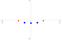
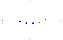
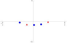
Figure 14: Examples of configurations with free holes for $N=8,M=3,\gamma=3,h=16$.

The above observation suggests a better definition of $\mathfrak{r}$: let $\mathfrak{r}^{\prime}$ be the ratio of the sum of $|\Lambda_{j}|$ over particle-hole excitations and free hole excitations to the sum of all $|\Lambda_{j}|$ in a given $s\neq 0$ sector. A list of values of $\mathfrak{r}^{\prime}$ for $N=10$ and $12$ is shown in Table 3.

	$N=10$		$N=12$
s	$\mathfrak{r}^{\prime}$	$n_{\text{pf}}/n_{\text{total}}$	$\mathfrak{r}^{\prime}$	$n_{\text{pf}}/n_{\text{total}}$
1	0.999	199/210	*	*
2	0.991	97/120	0.972	112/220
3	0.989	35/45	0.992	54/66

Table 3: The values of modified $\mathfrak{r}$ for $N=10$ and $12$. The symbol $n_{\text{pf}}$ means the sum of the number of particle-hole states plus that of the free hole states (avoiding double counts).

The above finite-$N$ numerical investigations all justify the claim in the main text: in the Trotter limit $N\rightarrow\infty$, in the presence of a finite magnetic field, the description of the excitations in terms of free holes and particle-hole pairs is complete at low temperatures.

B.3 Higher-level Bethe Ansatz equation in finite-N approximation

We demonstrate the accuracy of the higher-level Bethe Ansatz equations within the finite Trotter number approximation. Consider the 10th largest eigenvalue state of the quantum transfer matrix for $N=8$, $h=2$, $\gamma=2$ and $s=0$ at $T=0.46$. The precise locations of the Bethe roots and holes are given in Table 4. The root in the upper half plane is identified as a close root $x^{c}$. The hole with positive (negative) real part is labeled as $x^{h}_{1}$ ($x^{h}_{2}$). Clearly $x^{c}$ and $x^{h}_{1}$ constitute a 2-string:$\frac{x^{c}-x^{h}_{1}}{\gamma}=1.11508{\rm i}+0.0100447$.

Bethe roots	holes
$1.23901+1.09988{\rm i}(x^{c})$	$1.21892-1.13029{\rm i}(x^{h}_{1})$
$0.585152-0.979686{\rm i}$	$-0.385543-0.942574{\rm i}(x^{h}_{2})$
$0.0805622-0.956196{\rm i}$
$-1.07883-0.940606{\rm i}$

Table 4: The location of Bethe roots and holes in the complex plane for the 10th eigenvalue for $N=8$, $h=2$, $\gamma=2$ and $s=0$ at $T=0.46$.

To apply the higher-level Bethe Ansatz equation in finite $N$ approximation, we have to replace the dressed energy $\epsilon(x)$ by

$$\epsilon_{N}(x)=\frac{h}{2}+\frac{NT}{2}\ln\Biggl{(}\frac{\operatorname{cn}\bigl{(}\frac{2K}{\pi}(x-{\rm i}\frac{\beta}{N})\big{|}k\bigr{)}+{\rm i}\operatorname{sn}\bigl{(}\frac{2K}{\pi}(x-{\rm i}\frac{\beta}{N})\big{|}k\bigr{)}}{\operatorname{cn}\bigl{(}\frac{2K}{\pi}(x+{\rm i}\frac{\beta}{N})\big{|}k\bigr{)}+{\rm i}\operatorname{sn}\bigl{(}\frac{2K}{\pi}(x+{\rm i}\frac{\beta}{N})\big{|}k\bigr{)}}\Biggr{)}$$

which is obtained by replacing $\varepsilon_{0}$ by $\varepsilon_{0}^{(N)}$ (see (18), (27)) in (40). With $\varepsilon_{N}$ instead of $\varepsilon$ in (57) (and by setting $n_{+}=n_{-}=0$), the result in the main body of the paper claims that holes satisfy $\mathfrak{a}^{(0)}(x^{h}_{j})=-1\,(j=1,2)\,.$ Note that, for the present case, we have independently checked that $k=0$. The location of the close root is found to satisfy $\mathfrak{a}^{(0)}(x^{c})+\mathfrak{a}^{(+)}(x^{c})=-1$. For $N$ being finite, the first term disappears and the subsidiary condition simplifies to $\mathfrak{a}^{(+)}(x^{c})=-1\,.$ The numerical data in Table 5 indicate that they are satisfied with reasonable accuracy despite the fact that $N$ is not really large.

$\mathfrak{a}^{(0)}(x^{h}_{1})$	$-1.00126-0.00819979{\rm i}$
$\mathfrak{a}^{(0)}(x^{h}_{2})$	$-0.99882-0.00656583{\rm i}$
$\mathfrak{a}^{(+)}(x^{c})$	$-1.00025-0.0183492{\rm i}$

Table 5: The values of the finite-$N$ auxiliary functions in low-$T$ approximation at the exact numerical holes’ and particle’s positions given in Table 4. The parameters $N,h,\gamma,T$ are identical to those given there.

References

- [1] G. Albertini, S. Dasmahapatra, and B. M. McCoy, Spectrum and completeness of the integrable 3-state Potts model: A finite size study, Int. J. Mod. Phys. A 7 (1992), 1.
- [2] O. Babelon, H. J. de Vega, and C. M. Viallet, Analysis of the Bethe Ansatz equations of the XXZ model, Nucl. Phys. B 220 (1983), 13.
- [3] R. J. Baxter, One-dimensional anisotropic Heisenberg chain, Ann. Phys. (N.Y.) 70 (1972), 323.
- [4] , Partition function of the eight-vertex lattice model, Ann. Phys. (N.Y.) 70 (1972), 193.
- [5] M. Dugave, F. Göhmann, and K. K. Kozlowski, Thermal form factors of the XXZ chain and the large-distance asymptotics of its temperature dependent correlation functions, J. Stat. Mech.: Theor. Exp. (2013), P07010.
- [6] , Low-temperature large-distance asymptotics of the transversal two-point functions of the XXZ chain, J. Stat. Mech.: Theor. Exp. (2014), P04012.
- [7] M. Dugave, F. Göhmann, K. K. Kozlowski, and J. Suzuki, On form factor expansions for the XXZ chain in the massive regime, preprint, arXiv:1412.8217, 2014.
- [8] F. Göhmann, A. Klümper, and A. Seel, Integral representations for correlation functions of the XXZ chain at finite temperature, J. Phys. A 37 (2004), 7625.
- [9] , Integral representation of the density matrix of the XXZ chain at finite temperature, J. Phys. A 38 (2005), 1833.
- [10] M. Jimbo and T. Miwa, Algebraic analysis of solvable lattice models, American Mathematical Society, 1995.
- [11] J. D. Johnson, S. Krinsky, and B. M. McCoy, Vertical-arrow correlation length in the eight-vertex model and the low-lying excitations of the X-Y-Z Hamiltonian, Phys. Rev. A 8 (1973), 2526.
- [12] N. Kitanine, K. K. Kozlowski, J. M. Maillet, N. A. Slavnov, and V. Terras, A form factor approach to the asymptotic behavior of correlation functions in critical models, J. Stat. Mech.: Theor. Exp. (2011), P12010.
- [13] , The thermodynamic limit of particle-hole form factors in the massless XXZ Heisenberg chain, J. Stat. Mech.: Theor. Exp. (2011), P05028.
- [14] , Form factor approach to dynamical correlation functions in critical models, J. Stat. Mech.: Theor. Exp. (2012), P09001.
- [15] A. Klümper, Free energy and correlation length of quantum chains related to restricted solid-on-solid lattice models, Ann. Physik 1 (1992), 540.
- [16] , Thermodynamics of the anisotropic spin-1/2 Heisenberg chain and related quantum chains, Z. Phys. B 91 (1993), 507.
- [17] A. Klümper, J. R. Martinez, C. Scheeren, and M. Shiroishi, The spin-1/2 XXZ chain at finite magnetic field: Crossover phenomena driven by temperature, J. Stat. Phys. 102 (2001), 937.
- [18] A. Klümper and C. Scheeren, The thermodynamics of the spin-1/2 XXX chain: free energy and low-temperature singularities of correlation lengths, Classical and Quantum Nonlinear Integrable Systems (A. Kundu, ed.), Series in Mathematical and Computational Physics, IOP publishing, Bristol, 2003, pp. 234–255.
- [19] K. K. Kozlowski, J. M. Maillet, and N. A. Slavnov, Correlation functions for one-dimensional bosons at low temperature, J. Stat. Mech.: Theor. Exp. (2011), P03019.
- [20] M. Lashkevich, Free field construction for the eight-vertex model: representation for form factors, Nucl. Phys. B 621 (2002), 587.
- [21] S. Lukyanov, Correlation amplitude for the XXZ spin chain in the disordered regime, Phys. Rev. B 59 (1999), 11163.
- [22] S. Lukyanov and V. Terras, Long-distance asymptotics of spin-spin correlation functions for the XXZ spin chain, Nucl. Phys. B 654 (2003), 323.
- [23] K. Sakai, M. Shiroishi, J. Suzuki, and Y. Umeno, Commuting quantum transfer matrix approach to intrinsic Fermion system: Correlation length of a spinless Fermion model, Phys. Rev. B 60 (1999), 5186.
- [24] J. Suzuki, Y. Akutsu, and M. Wadati, A new approach to quantum spin chains at finite temperature, J. Phys. Soc. Jpn. 59 (1990), 2667.
- [25] M. Suzuki, Transfer-matrix method and Monte Carlo simulation in quantum spin systems, Phys. Rev. B 31 (1985), 2957.
- [26] M. Suzuki and M. Inoue, The ST-transformation approach to analytic solutions of quantum systems. I. General formulations and basic limit theorems, Prog. Theor. Phys. 78 (1987), 787.
- [27] M. Takahashi, Correlation length and free energy of the XYZ chain, Phys. Rev. B 43 (1991), 5788.
- [28] A. Virosztek and F. Woynarovich, Degenerated ground states and excited states of the anisotropic antiferromagnetic Heisenberg chain in the easy axis region, J. Phys. A 17 (1984), 3029.
- [29] E. T. Whittaker and G. N. Watson, A course of modern analysis, fourth ed., ch. 21, Cambridge University Press, 1963.
- [30] F. Woynarovich, On the =0 excited states of an anisotropic Heisenberg chain, J. Phys. A 15 (1982), 2985.
- [31] C. N. Yang and C. P. Yang, One-dimensional chain of anisotropic spin-spin interactions. III. Applications, Phys. Rev. 151 (1966), 258.