Hyperspherical theory of the quantum Hall effect: the role of exceptional degeneracy

Abstract

By separating the Schrödinger equation for $N$ noninteracting spin-polarized fermions in two-dimensional hyperspherical coordinates, we demonstrate that fractional quantum Hall (FQH) states emerge naturally from degeneracy patterns of the antisymmetric free-particle eigenfunctions. In the presence of Coulomb interactions, the FQH states split off from a degenerate manifold and become observable as distinct quantized energy eigenstates with an energy gap. This alternative classification scheme is based on an approximate separability of the interacting $N$-fermion Schrödinger equation in the hyperradial coordinate, which sheds light on the emergence of Laughlin states as well as other FQH states. An approximate good collective quantum number, the grand angular momentum $K$ from $K$-harmonic few-body theory, is shown to correlate with known FQH states at many filling factors observed experimentally.

I Introduction

One of the most striking aspects of nonrelativistic quantum mechanics in more than one dimension is the remarkable implication of high degeneracy or near-degeneracy. Textbook examples include the sp-hybridization of chemical bonds and the degenerate Stark effect of excited hydrogen atoms. In the degenerate Stark effect, for instance, even an infinitesimally small external electric field selects energy eigenstates that are linear combinations of a finite set of degenerate zero-field states, and these are the same eigenstates that can be obtained by separating the field-free Schrödinger equation for that system in parabolic coordinates.

A major development presented in this article is that similar considerations apply to the fractional quantum Hall effect (FQHE) Tsui et al. (1982); Stormer et al. (1999). In the fractional quantum Hall effect, a strongly-interacting two-dimensional electron gas exhibits quantization in the presence of a strong, perpendicular magnetic field. In the noninteracting limit, the electrons fall into highly degenerate Landau levels, and their collective behavior depends on the filling factor, the ratio of the number of electrons to the large, but finite, degeneracy of the lowest Landau level for a sample with finite area. The system exhibits quantization when the filling factor takes on integer or certain rational fraction values. We show that the high degeneracy of the noninteracting system produces dramatic implications.

Moreover, we demonstrate that the N-electron Schrödinger equation is approximately separable in hyperspherical coordinates. This approach to the problem shows that a characteristic property of the noninteracting system, which we denote the exceptional degeneracy, becomes unusually high for precisely those states that appear at experimentally and theoretically observed FQHE filling factors. In other words, even though the FQHE is viewed fundamentally as the epitome of a strongly-correlated system of electrons, the occurrence or nonoccurrence of a FQHE filling factor is highly correlated with the pattern of exceptional degeneracies in the noninteracting electron system. The approximate separability demonstrated in hyperspherical coordinates for the few-body quantum Hall states makes definite predictions about a class of excitation frequencies that could be used to experimentally probe the system.

Extensive progress in the theoretical understanding of the FQHE has been achieved through various approaches following the early intuitive development by Laughlin Laughlin (1983a), notably the composite fermion (CF) picture developed by Jain Jain (1989, 2007), and work by Haldane Haldane (1983), and Halperin Halperin (1984). Theoretical treatments have tended to reside in one of two different categories, either postulating trial wavefunctions as in Laughlin’s original approach, (e.g. Moore and Read (1991); Ginocchio and Haxton (1996); Wójs et al. (2004)) or else performing large numerical diagonalizations for the maximum number of electrons that can still give a manageable size computation, typically 8-20 particles (e.g. Haldane and Rezayi (1985)). A more recently developed technique uses CF wave functions as a basis for numerical diagonalization to study systems with larger numbers of particles Jeon et al. (2007); Mukherjee et al. (2014).

The approach developed here has some advantages complementary to previous methods. In contrast to techniques that use the single-particle representation (i.e. Slater determinant constructions), the approach treated here inherently uses collective coordinates. It also provides a systematic expansion that can in principle describe any states existing in the Hilbert space of a finite number of particles, while at the same time allowing us to see many key properties analytically or with small-scale diagonalizations. The adiabatic hyperspherical representation capitalizes on an approximate separability, and its key element is a set of potential energy curves showing at a glance the relevant size and energy of different energy eigenstates. While the hyperradial degree of freedom is not separable for arbitrarily strong Coulomb interactions, our calculations demonstrate that approximate Born-Oppenheimer separability is an excellent approximation in typical regimes of electron density and field strength for a typical material like GaAs.

While the adiabatic hyperspherical representation Macek (1968); Fano (1981, 1983) has not been used extensively in condensed matter theory, it has had extensive success in a wide range of few-body contexts. The literature in this field documents theoretical results that have been achieved in contexts as diverse as nuclear structure and reactivity Smirnov and Shitikova (1977); Avery (1989, 1993); Nielsen et al. (2001); Daily et al. (2015a), universal Efimov physics in cold atoms and molecules Wang et al. (2013); Rittenhouse et al. (2011); Wang et al. (2014); Efimov (1970); Nielsen and Macek (1999); Gattobigio et al. (2012), few-electron atoms Lin (1986, 1995); Lin and Morishita (2000), and systems containing positrons and electrons Botero and Greene (1985); Daily and Greene (2014); Daily et al. (2015b); Archer et al. (1990). Efimov’s prediction Efimov (1970) of a universal binding mechanism for three particles at very large scattering lengths can itself be viewed as an application of the adiabatic hyperspherical coordinate treatment in a problem where the method is exact, although Efimov did not himself express it in those terms. Hyperspherical coordinates have also been employed to describe some many-body phenomena such as the trapped atom Bose-Einstein condensate with either attractive or repulsive interactions Bohn et al. (1998); Kushibe et al. (2004) and the trapped degenerate Fermi gas in three dimensions including the BCS-BEC crossover problem. Rittenhouse et al. (2006, 2011)

Our initial presentation of the formulation begins by setting up the problem rigorously for N electrons confined to a plane with a transverse uniform magnetic field. The antisymmetric states for spin-polarized fermions are found directly using the technique developed in Ref. Efros (1995). Next we show that the exact separability of the Schrödinger equation in hyperspherical coordinates for the case of noninteracting electrons still exhibits an approximate separability even in the presence of Coulomb interactions. The treatment then demonstrates how interactions single out potential energy curves or channels of exceptional degeneracy, which correlate with known Laughlin states, composite fermion FQHE states, and suggest other states that deserve future theoretical and experimental investigation. This enables further predictions of a class of excitation frequencies that should be experimentally observable in a FQHE experiment.

This paper is organized as follows. Sections II and III formulate the one-body and N-body relative Hamiltonians in the symmetric gauge. Section IV defines the hyperspherical coordinates adopted in the present study and writes the unsymmetrized hyperspherical harmonics which serve as our primitive basis set. This basis set is then connected to the Landau level picture and suggests a definition for the hyperspherical filling factor. The effect of Coulomb interactions is then developed and treated within the adiabatic hyperspherical representation. Section V introduces the concept of exceptional degeneracy and computes this key quantity, which correlates with filling factors that are observable as FQH ground states. Section VI offers concluding remarks and comments on future directions. Finally, Appendix A relates the states with different hyperspherical filling factors to several of the states that have previously been identified in the conventional composite fermion picture.

II Single particle Hamiltonian,

The noninteracting Hamiltonian $H$ for a single electron in an external magnetic field is given by

$$H=\frac{1}{2m_{e}}\left(-\imath\hbar\bm{\nabla}+e\bm{A}\right)^{2}$$ (1)

in SI units where $m_{e}$ is the effective mass of the electron in the medium, $e$ is the magnitude of the electron charge, $\hbar$ is Planck’s constant, and $\bm{A}$ is the vector potential. For two dimensional space, in Cartesian coordinates, the gradient is $\bm{\nabla}=\hat{x}\partial_{x}+\hat{y}\partial_{y}$. For a constant magnetic field of magnitude $B$ oriented in the positive $\hat{z}$ direction, the vector potential is $\bm{A}=(B/2)(-y\hat{x}+x\hat{y})$. Expanding Eq. (1) with this choice of $\bm{A}$ yields

$$H=-\frac{\hbar^{2}}{2m_{e}}\bm{\nabla}^{2}+\frac{e^{2}B^{2}}{8m_{e}}(x^{2}+y^{2})+\frac{eB}{2m_{e}}L_{z},$$ (2)

where $L_{z}$ is the $z$-component of the angular momentum operator, $L_{z}=-\imath\hbar(x\partial_{y}-y\partial_{x})$.

The rest of this paper uses magnetic units where length is expressed in units of $\lambda_{0}$,

$$\lambda_{0}=\sqrt{\frac{\hbar}{m_{e}\omega_{c}}}$$ (3)

and energy is expressed in units of $\hbar\omega_{c}$, where $\omega_{c}$ is the cyclotron frequency, $\omega_{c}=eB/m_{e}$. In these units, expressing $H$ in polar coordinates yields

$$H=-\frac{1}{2}\left\{\frac{1}{r}\partial_{r}r\partial_{r}-\frac{L_{z}^{2}}{\hbar^{2}r^{2}}\right\}+\frac{1}{8}r^{2}+\frac{1}{2\hbar}L_{z},$$ (4)

and the single-particle energy $E^{(1)}$ is

$$E^{(1)}=\frac{1}{2}\left(2n+m+|m|+1\right),$$ (5)

where $n$ is a nodal quantum number and $m$ is the rotational quantum number about the $z$-axis. Section III shows how the Hamiltonian is modified when including more degrees of freedom, while Sec. IV.3 makes additional modifications when expressed in hyperspherical coordinates. Many aspects of Eqs. (4) and (5) carry over to this formalism.

III N-body relative Hamiltonian

The $N$-body noninteracting Hamiltonian $H_{N}$ is separable into a center of mass $H_{\rm CM}$ and relative $H_{\rm rel}$ components,

$$H_{N}=H_{\rm CM}+H_{\rm rel},$$ (6)

where, in Cartesian coordinates akin to Eq. (2),

$$H_{\rm rel}= -\frac{1}{2\mu}\sum_{j=1}^{N_{\rm rel}}\bm{\nabla}_{j}^{2}+\frac{\mu}{8}\sum_{j=1}^{N_{\rm rel}}(x_{j}^{2}+y_{j}^{2})+\frac{1}{2\hbar}\sum_{j=1}^{N_{\rm rel}}L_{z_{j}}^{\rm rel}.$$ (7)

Here, $N_{\rm rel}=N-1$ is the number of relative Jacobi vectors $\bm{\rho}_{j}$ with Cartesian components $x_{j}$ and $y_{j}$, and $\mu$ is a dimensionless mass scaling factor Delves (1959, 1960),

$$\mu=\left(\frac{1}{N}\right)^{1/N_{\rm rel}}.$$ (8)

The center-of-mass Hamiltonian is similar in form to Eq. (7), except $\mu$ is replaced by $N$ and there is only the center-of-mass vector $\bm{\rho}_{\rm CM}$.

The linear transformation from single-particle to center-of-mass and relative Jacobi vectors is arbitrary, but in this work, the scheme used first joins identical particles into pairs, then joins the center of mass of each pair into ever larger clusters. For odd $N$, the unpaired electron is joined to the center of mass of the other paired particles. The Jacobi vectors are labeled in a reverse manner, so that the last Jacobi vector, the $(N-1)^{st}$, is always the relative coordinate for a pair of particles, and where the Jacobi vectors of the largest clusters have the smallest index. For example, for five electrons in matrix notation this is

$$\begin{pmatrix}\bm{\rho}_{1}\\ \bm{\rho}_{2}\\ \bm{\rho}_{3}\\ \bm{\rho}_{4}\\ \bm{\rho}_{\rm CM}\end{pmatrix}=\left(\!\!\!\!\begin{array}[]{rlcccr}\sqrt{\frac{4/5}{\mu}}\times&\{\frac{1}{4}&\frac{1}{4}&\frac{1}{4}&\frac{1}{4}&-1\}\\ \sqrt{\frac{1}{\mu}}\times&\{\frac{1}{2}&\frac{1}{2}&-\frac{1}{2}&-\frac{1}{2}&0\}\\ \sqrt{\frac{1/2}{\mu}}\times&\{0&0&1&-1&0\}\\ \sqrt{\frac{1/2}{\mu}}\times&\{1&-1&0&0&0\}\\ \frac{1}{5}\times&\{1&1&1&1&1\}\end{array}\right)\!\!\begin{pmatrix}\bm{r}_{1}\\ \bm{r}_{2}\\ \bm{r}_{3}\\ \bm{r}_{4}\\ \bm{r}_{5}\end{pmatrix}\!\!.$$ (14)

Figure 1

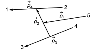
Figure 1: (Color online) Diagram describing the mass-scaled Jacobi coordinates of Eq. (14).

is a diagrammatic representation of the Jacobi vectors described by Eq. (14). The numbers denote particle locations while the arrows denote the Jacobi vectors, also labeled by $\bm{\rho}_{j}$. This choice of Jacobi tree reduces the size of the unsymmetrized basis needed to achieve antisymmetric states, as is described in Sec. IV.2.

IV Hyperspherical form

This section describes the hyperspherical transformation of the noninteracting relative Hamiltonian, how the relative Hamiltonian is expressed in these coordinates, and the resulting adiabatic potentials.

IV.1 Hyperspherical coordinate transformation

Hyperspherical coordinates are the generalization of spherical coordinates beyond three degrees of freedom. The size of the system is correlated with a single length, the hyperradius $R$, while the geometry of the system is encoded in the remaining degrees of freedom as a set of hyperangles, denoted by $\bm{\Omega}$. This length $R$,

$$R^{2}=\sum_{j=1}^{N_{\rm rel}}\rho^{2}_{j},$$ (15)

is a scalar quantity and its square is the sum of the squared lengths of the Jacobi vectors.

The orthogonal coordinate transformation from Cartesian to hyperspherical coordinates has some arbitrariness, and many different schemes can be found in the literature Smirnov and Shitikova (1977); Avery (1989, 1993); Rittenhouse et al. (2011). In this work, the semi-canonical construction is most useful [see also Fig. A4 of Ref. Rittenhouse et al. (2011)]. It resembles the canonical tree structure of Refs. Smirnov and Shitikova (1977); Avery (1989), but instead of each new branch adding a single degree of freedom, each additional branch adds an additional two-dimensional sub-tree. In this way, the particle-like nature of the two-dimensional Jacobi vectors is maintained. This set of hyperangles consists of the $N_{\rm rel}$ azimuthal angles $\phi_{j}$ associated to each Jacobi vector $\bm{\rho}_{j}$ and the $N_{\rm rel}-1$ constructed hyperangles $\alpha_{j}$, where

$$\tan\alpha_{j}=\frac{\sqrt{\sum_{k=1}^{j}\rho_{k}^{2}}}{\rho_{j+1}}.$$ (16)

Figure 2

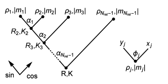
Figure 2: (Color online) Semi-canonical Jacobi tree diagram. The sub-tree in the lower right describes the $N_{\rm rel}-1$ nodes at the top of the main tree. Reading from the main node at $R,K$, any time a node is passed to the left (right), the coordinate picks up a factor of $\sin\alpha_{j}$ ($\cos\alpha_{j}$).

gives a diagrammatic representation of the semi-canonical construction. This Jacobi tree connects branches (segments) into nodes (dots), where to every node is associated a sub-length, a sub-hyperangular quantum number [see e.g. Eq. (24)], and an angle. The sub-lengths $R_{j}$ are defined similarly to Eq. (15), e.g. $R_{2}^{2}=\rho_{1}^{2}+\rho_{2}^{2}$.

The Jacobi tree contains all of the information describing the coordinate transformation from Cartesian to hyperspherical. Read from the main node at $\{R,K\}$ to the top nodes at $\{\rho_{j},|m_{j}|\}$, any time a node is passed to the left (right), the Cartesian coordinate picks up a factor of $\sin\alpha_{j}$ ($\cos\alpha_{j}$). The sub-tree in the lower right of Fig. 2 describes the $N_{\rm rel}-1$ nodes at the top of the main tree. For example, $x_{1}=\rho_{1}\cos\phi_{1}$. However, for $N=5$, $x_{1}$ in terms of every node is expressed as $x_{1}=R\sin\alpha_{3}\sin\alpha_{2}\sin\alpha_{1}\cos\phi_{1}$. The $\phi_{j}$ angles range from $0<\phi<2\pi$ while the hyperangles $\alpha_{j}$ range from $0<\alpha_{j}<\pi/2$. The volume element for each $\phi_{j}$ is $d\phi_{j}$, while for each $\alpha_{j}$ it is $\sin^{2j-1}\alpha_{j}\cos\alpha_{j}d\alpha_{j}$.

IV.2 Relative Hamiltonian

The noninteracting relative Hamiltonian, Eq. (7), transforms to

$$H_{\rm rel}=-\frac{1}{2\mu}\bm{\nabla}^{2}_{R,{\bm{\Omega}}}+\frac{\mu}{8}R^{2}+\frac{1}{2\hbar}L_{z}^{\rm rel,tot}$$ (17)

where $L_{z}^{\rm rel,tot}$ is the total relative $z$-component of the angular momentum, and the Laplacian operator in hyperspherical coordinates $\bm{\nabla}^{2}_{R,{\bm{\Omega}}}$ becomes

$$\bm{\nabla}^{2}_{R,{\bm{\Omega}}}=\frac{1}{R^{2N_{\rm rel}-1}}\partial_{R}R^{2N_{\rm rel}-1}\partial_{R}-\frac{\hat{\bm{K}}^{2}}{R^{2}}.$$ (18)

$\hat{\bm{K}}$ is called the grand angular momentum operator Avery (1989). Note the similarity with Eq. (4), where there are radial and angular components.

The eigenstates of $\hat{\bm{K}}^{2}$ are the hyperspherical harmonics, $\Phi_{K{u}}^{(M)}(\bm{\Omega})$, where

$$\hat{\bm{K}}^{2}\Phi_{K{u}}^{(M)}(\bm{\Omega})=K(K+2N_{\rm rel}-2)\Phi_{K{u}}^{(M)}(\bm{\Omega})$$ (19)

and the set of hyperspherical harmonics are orthonormal over the hyperangles $\bm{\Omega}$,

$$\int d\bm{\Omega}\;\Phi_{K^{\prime}{u}^{\prime}}^{(M)*}(\bm{\Omega})\Phi_{K{u}}^{(M)}(\bm{\Omega})=\delta_{K^{\prime}K}\delta_{{u}^{\prime}{u}}.$$ (20)

The grand angular momentum quantum number $K$ ($K=0,1,2,\ldots$) is analogous to the angular momentum quantum number; for the noninteracting system, it remains a good quantum number. Here, $u$ is an index used to label the different unsymmetrized states within a given $K$-manifold (fixed $K$ subspace). For $2N_{\rm rel}$ degrees of freedom, there are $(2N_{\rm rel}-2+2K)(2N_{\rm rel}-3+K)!/(K!(2N_{\rm rel}-2)!)$ linearly independent unsymmetrized functions.

The projection quantum numbers $m_{j}$ associated with the Jacobi vectors are not good quantum numbers in the presence of interactions and antisymmetrization, however the total projection quantum number $M$ remains a good quantum number of the system, even with Coulomb interactions (or any other interactions that depend only on the inter-particle distances). The set of hyperspherical harmonics are made simultaneous eigenstates of $\hat{\bm{K}}^{2}$ and $L_{z}^{\rm rel,tot}$ by enforcing the constraint

$$\sum_{j=1}^{N_{\rm rel}}m_{j}=M,$$ (21)

$|M|\leq K$, which is assumed in the following discussion. Because the center of mass has already been separated, it does not contribute to $M$, and its $L_{z}$ and energy can be incorporated into the system trivially.

In the semi-canonical coupling scheme of this work (see Fig. 2), the unsymmetrized hyperspherical harmonics are expressed as

$$\Phi_{K{u}}^{(M)}(\bm{\Omega})= \prod_{j=1}^{N_{\rm rel}}\frac{e^{\imath m_{j}\phi_{j}}}{\sqrt{2\pi}}\prod_{k=1}^{N_{\rm rel}-1}{\cal N}_{k}\;\sin^{K_{k}}\alpha_{k}\;\cos^{|m_{k+1}|}\alpha_{k}\;P_{n_{k}}^{K_{k}+(k-1),|m_{k+1}|}(\cos 2\alpha_{k}),$$ (22)

$${\cal N}_{k}^{2}=\frac{(2K_{k+1}+2k)\;\Gamma(n_{k}+K_{k}+|m_{k+1}|+k)\;\Gamma(n_{k}+1)}{\Gamma(n_{k}+K_{k}+k)\;\Gamma(n_{k}+|m_{k+1}|+1)},$$ (23)

where the $P$ are Jacobi polynomials, ${\cal N}_{k}$ is the normalization for each Jacobi polynomial, and the $K_{k}$ are sub-hyperangular “quantum numbers,” defined recursively as

$$K_{1} =|m_{1}|,\mbox{ and}$$ (24)

$$K_{k} =2n_{k-1}+K_{k-1}+|m_{k}|.$$ (25)

The $n_{k}$ ($n_{k}=0,1,2,\ldots$) are determined after fixing the various $K_{k}$ and $|m_{k}|$. In practice, it is easier to first choose the $n_{k}$ and $|m_{k}|$, since $n_{k}$ is the order of the Jacobi polynomial, then determine the $K_{k}$.

With the exception of the grand angular momentum $K$ and the total azimuthal quantum number $M$, neither the $K_{k}$ nor the $m_{k}$ remain good quantum numbers after antisymmetrizing the hyperspherical harmonics. We antisymmetrize the set of functions Eq. (22) following the method of Ref. Efros (1995). In a closed subspace of the Hamiltonian (here, the subspaces with both fixed $K$ and fixed $M$), the antisymmetrized states must be linear combinations of the unsymmetrized basis functions within the same subspace. As before, the subscript ${u}$ is an index that distinguishes different orthogonal basis functions in the same manifold; each index ${u}$ is associated with a different set of good hyperspherical quantum numbers that satisfy Eqs. (24). Similarly, the new subscript $a$ will later be used to index different antisymmetric states in the same manifold, but in this case, the $K_{k}$ and $m_{k}$ no longer constitute good quantum numbers. The complete set of basis function labels in the unsymmetrized basis will be indicated by a bold $\bm{u}=\{1,2,\ldots\}$, and the number of basis functions will be given by $|\bm{u}|$.

The antisymmetric basis functions can be constructed by first building the full matrix of the antisymmetrization operator $\hat{\mathcal{A}}=1-\hat{P}_{12}-\hat{P}_{13}-\hat{P}_{23}+\hat{P}_{123}+...$ (all $N!$ terms) connecting all unsymmetrized states $\Phi_{Ku}^{(M)}$ in a given $K,|M|$ manifold. This Hermitian matrix $\mathcal{A}_{ij}=\left\langle\Phi_{Ki}^{(M)}|\mathcal{A}|\Phi_{Kj}^{(M)}\right\rangle$ is then diagonalized, i.e. we find the eigenvalues and their corresponding eigenvectors, $X_{ia}$. The $\overline{\mathcal{N}_{a}}$ eigenvectors with eigenvalues equal to $N!$ give the totally antisymmetric hyperangular wave functions,

$$\Phi_{Ka}^{(M)}=\sum_{u}\Phi_{Ku}^{(M)}X_{ua},\quad\quad a=1,2,...\overline{\mathcal{N}_{a}},$$ (26)

where $\overline{\mathcal{N}_{a}}$ is the number of antisymmetric states and is typically smaller than the total dimension of the degenerate unsymmetrized subspace. Note that the matrix $X$ depends of course on $K$ and $M$, but this has been suppressed for notational brevity.

The most time-consuming part of this calculation is the determination of the matrix $\mathcal{A}_{ij}$, which can be accomplished using a technique proposed by Efros Efros (1995). Instead of being calculated directly, the antisymmetrization matrix can be found by treating $\mathcal{A}_{ij}$ as many unknowns in a linear system of equations. The antisymmetrization matrix is first re-expressed in terms of a matrix equation,

$${\cal\hat{A}}\Phi_{Kj}^{(M)}(\bm{\Omega})=\sum_{i}\Phi_{Ki}^{(M)}(\bm{\Omega})\mathcal{A}_{ij},$$ (27)

where $i,j\in{\bm{u}}$ and $\Phi_{Kj}^{(M)}(\bm{\Omega})$ represents a $|\bm{u}|$-length row array of all of the unsymmetrized basis functions. The matrix $\mathcal{A}_{ij}$ is the unknown $|\bm{u}|\times|\bm{u}|$ matrix representation of the antisymmetrization operator, and Eq. (27) evaluated at a single set of $N$-particle coordinates constitutes a system of $|\bf{u}|$ equations with ${\bm{u}^{2}}$ unknowns. The antisymmetrization operator is understood to act on the particle coordinates, so that ${\cal\hat{A}}\Phi_{Kj}^{(M)}(\bm{\Omega})=\Phi_{Kj}^{(M)}({\cal\hat{A}}\bm{\Omega})$

Because Eq. (27) holds true for any set of N-particle coordinates, substituting any random set of angular coordinates ${\bm{\Omega}}_{\gamma}$ produces a different, linearly independent equation in the unknowns of the antisymmetrization matrix, $\mathcal{A}_{ij}$. Substituting $|\bf{u}|$ different sets of $N$-particle coordinates into Eq. (27) results in a linear system of equations that can be solved for $\mathcal{A}_{ij}$. If we write $\Phi_{\gamma j}$ to mean the two-dimensional array of unsymmetrized basis functions evaluated at different sets of $N$-particle coordinates, where the column index $j$ indexes the $|{\bm{u}}|$ different unsymmetrized basis functions, the row index $\gamma$ indexes the $|{\bm{u}}|$ different sets of coordinates, ${\bm{\Omega}}_{\gamma}$, and the $K$ and $M$ quantum numbers have been suppressed, then $\mathcal{A}_{ij}$ can be found by solving the following equation:

$$\hat{\mathcal{A}}\Phi_{\gamma j}=\sum_{i}\Phi_{\gamma i}\mathcal{A}_{ij}.$$ (28)

In practice, constructing the matrices $\Phi_{\gamma i}$ and $\hat{\mathcal{A}}\Phi_{\gamma j}$ is trivially parallelizable, but the memory requirements are significant since it requires the storage of two $|\bm{u}|\times|\bm{u}|$ double complex dense matrices. The size of the unsymmetrized basis increases dramatically with the number of particles. Choosing paired Jacobi coordinates helps limit the growth in spin-polarized fermion systems, since states with pair coordinates associated with even $m_{j}$ can be eliminated due to symmetry. However, the growth is still rapid, and as a result we have only performed calculations in systems with up to 6 spin-polarized electrons at $1/3$ filling. In the future, with programs like SCALAPACK, it is feasible to push this analysis further. The problem of antisymmetrizing the hyperspherical functions becomes very challenging as unsymmetrized basis expands, and other strategies for antisymmetrization may also prove effective Barnea (1999); Krivec (1998); Viviani (1998).

IV.3 Eigenstates of the noninteracting $H_{\rm rel}$

Each exact eigenfunction $\Psi(R,\bm{\Omega})$ of the relative Hamiltonian, Eq. (17), is separable into a hyperradial function, $F_{n_{R}K}^{(M)}(R)$, and one antisymmetrized hyperspherical harmonic ,$\Phi_{Ka}^{(M)}(\bm{\Omega})$,

$$\Psi(R,\bm{\Omega})=R^{-N_{\rm rel}+1/2}F_{n_{R}K}^{(M)}(R)\Phi_{K{a}}^{(M)}(\bm{\Omega}).$$ (29)

The many-dimensional hyperradial Schrödinger equation thus reduces to a one-dimensional uncoupled ordinary differential equation:

$$\left\{-\frac{1}{2\mu}\frac{d^{2}}{dR^{2}}+U_{K}^{(M)}(R)-E\right\}F_{n_{R}K}^{(M)}(R)=0,$$ (30)

where the noninteracting potentials $U_{K}^{(M)}(R)$ are given by

$$U_{K}^{(M)} (R)=$$ (31)

$$\frac{(K+N_{\rm rel}-1/2)(K+N_{\rm rel}-3/2)}{2\mu R^{2}}+\frac{\mu}{8}R^{2}+\frac{1}{2}M.$$

The noninteracting hyperradial solutions $F_{n_{R}K}^{(M)}(R)$ to the scaled Schrödinger equation, Eq. (30), are

$$F_{n_{R}K}^{(M)}(R)={\cal N}e^{-\tfrac{\mu R^{2}}{4}}L_{n_{R}}^{K+N_{\rm rel}-1}\left(\frac{\mu R^{2}}{2}\right)R^{K+N_{\rm rel}-1/2},$$ (32)

where $n_{R}$ $(n_{R}=0,1,2,\ldots)$ is the hyperradial quantum number and $L$ is the associate Laguerre polynomial. The normalization, where $\int_{0}^{\infty}|F_{n_{R}K}^{(M)}(R)|^{2}dR=1$, is

$${\cal N}=\sqrt{\frac{n_{R}!\;\mu^{K+N_{\rm rel}}}{\Gamma(n_{R}+K+N_{\rm rel})\;2^{K+N_{\rm rel}-1}}}.$$ (33)

The noninteracting many-body energies $E^{\rm NI}$ are

$$E^{\rm NI}=\frac{1}{2}(2n_{R}+M+K+N_{\rm rel}).$$ (34)

Note that this equation is similar in form to Eq. (5) where $n_{R}$ is a nodal quantum number and $K$ plays the role of the $|M|$ term. In the limit that $N_{\rm rel}=1$, this equation reduces to Eq. (5).

Figure 3

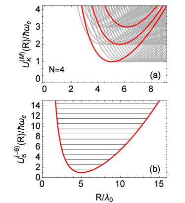
Figure 3: (Color online) (a) Light solid lines show the adiabatic potential curves of the noninteracting four-body system whose minima lie below $4\hbar\omega_{c}$. The lowest group ($K=|M|$) represents the lowest Landau level. The next and next-next higher groups are for $K=|M|+2$ and $K=|M|+4$, respectively. The dark solid lines are for $M=-6$, the lowest of which supports the integer quantum Hall state. (b) The $M=-6$ hyperradial noninteracting potential curve in the lowest Landau level and the corresponding hyperradial energy spectrum.

shows the effective potentials $U_{K}^{(M)}(R)$, Eq. (31), for the noninteracting system with four identical fermions. The light solid lines show all the potentials visible in the given scale, while the dark solid lines highlight those curves with $M=-6$ and, from bottom to top, $K=6,8,$ and $10$, respectively. One striking feature is that the potentials group into “bands” whose potential minima group around the same energy. Each band is separated by a cyclotron unit of energy, reminiscent of Landau levels. However, these potentials are not single-particle potentials, but rather support many-body states. In the case of Figure 3a, energy arguments indicate the first excited “band” represents a four-body state with a filled lowest Landau level and an excited electron.

For any $K,M$, the particles are confined due to the diamagnetic term and each of these potentials supports an infinite number of bound states. The noninteracting hyperradial solutions, Eq. (32), are centered within the non-inteacting potential wells, $U_{K}^{(M)}(R)$. For a given potential, each nodal excitation in the hyperradius adds one unit of cyclotron energy $\hbar\omega_{c}$, as shown in Fig. 3b, and the additional hyperradial nodes increase the overall size of the hyperradial wave function due to the additional hyperradial nodes. For a fixed $M$, the allowed values of $K$ are $K=|M|,|M|+2,\ldots$ in step sizes of 2. For each increase in $K$, the confining potential moves out in the hyperradius, indicating the size of the system is increasing as the energy increases.

Another striking feature is the potential that corresponds to the integer quantum Hall state. The dark curve with $K=|M|$, whose minimum is about $R\approx 5\lambda_{0}$, is isolated from the other curves with higher $K=|M|$ values. In fact, there is always a single isolated curve separated from the other curves at $K=|M|=N(N-1)/2$ for all system sizes. The one antisymmetric hyperspherical wave function of this manifold, when re-expressed in terms of independent particle coordinates, is exactly identical to the wave function of the integer quantum Hall state. Moreover, the first excited “band”, representing a filled lowest Landau level and an excited electron, allows potentials at smaller $K$ values. Exciting a single electron to a higher Landau level, allows the system to compress to a smaller hyperradius at the cost of one $\hbar\omega_{c}$ unit of energy.

IV.4 Hyperspherical filling factor

The most important parameter in the quantum Hall problem is the filling factor, $\nu$, the number of occupied Landau levels in a sample in the noninteracting limit. It is given by

$$\nu=\frac{\rho h}{eB}=\frac{N\phi_{0}}{BA},$$ (35)

where $\rho$ is the two-dimensional electron density, $B$ is the magnetic field, $N$ is the number of electrons, $A$ is the sample area, and $\phi_{0}$ is the fundamental flux quantum, $\phi_{0}=h/e$ in S.I. units Jain (2007). The filling factor gives the ratio of the number of electrons in the system to the number of available single particle orbitals in the lowest Landau level for a given sample area. The electron density can be somewhat controlled with doping and gate voltages, but for typical experiments in gallium arsenide Tsui et al. (1982); Pan et al. (2008) is on the order of $1-3\times 10^{11}cm^{-2}$. As an example, in a system with $\rho=2.4\times 10^{11}cm^{-2}$ Eisenstein and Stormer (1990), the $\nu=1$ quantum Hall state is found at a magnetic field near $B=10$T and the $\nu=1/3$ state occurs around the much higher field $B\approx 29$T.

Experimentally, the Hall resistance quantizes to values of $R_{H}=h/\nu e^{2}$. Defining the filling factor in terms of the electron density is ideal for experimental systems, where the local electron density is averaged over enormous numbers of electrons. However, for systems with few electrons, there is some reasonable ambiguity in establishing the average density of a sample that is not sharply confined. In most numerical models of the planar system, the ambiguity about the area is resolved by cutting out of the Hilbert space all single-particle wave-functions whose maxima in the lowest Landau level lies outside of a certain radius. The area of the disk defined by this radius is an approximate area for the few-particle model system.

In the hyperspherical construction, the area of a distribution of $N$ identical mass particles correlates with the particles’ hyperradius, Eq. (15), which can be used to define the filling factor without reference to the single particle wave functions. The connection between the hyperradius and the area can be established by a statistical average over a large ensemble of systems, holding the particle number $N$, and the sample radius, $r_{c}$ constant. Each individual system in the ensemble consists of a random distribution of $N$ particles over a disk with radius $r_{c}$. The particle density over this area is clearly $\rho=N/\pi r_{c}^{2}$, although the density is obviously non-uniform.

In general, systems with different random distributions of $N$ particles will have different hyperradii, but the value of the hyperradius squared tends to increase on average with increasing particle density and tends to decrease with disk size. The statistical average of the hyperradius squared for a fixed $N$ and $\pi r_{c}^{2}$ over many trials is empirically found to be

$$\langle R^{2}\rangle_{N,r_{c}}=\frac{(N-1)r_{c}^{2}}{2\mu},$$ (36)

where $\mu$ is the reduced mass of $N$ particles, Eq. (8). For any individual distribution of $N$ particles on a circle of radius $r_{c}$, Eq. (36) typically does not reproduce $r_{c}$ accurately. However, the definition of the particle density is also only described as an average. The particle density $\rho=N/\pi r_{c}^{2}$ for a few particles on a disk also does not actually give the average density of those particles except with reference to a statistical average. The hyperradius gives a consistent way to measure an approximate area of a distribution of particles, even in the less clearly defined case of very few particles.

Using Eq. (36), it is straightforward to find a hyperspherical expression for the filling factor. We first scale all lengths in the problem by the magnetic length of the system, $\lambda_{0}$ [see Eq. (3)], and get the filling factor in terms of the radius of a disk, $r_{c}$, that gives an approximate area of the sample. Substituting for this characteristic disk radius, equation Eq. (35) becomes

$$\nu=\frac{N(N-1)}{\mu\langle R^{2}\rangle}.$$ (37)

This expression for the filling factor can be used to distinguish the filling factors of different noninteracting wave functions. In the lowest Landau level, the (unnormalized) noninteracting hyperradial wave functions have no hyperradial excitations and depend very simply on the hyperradius and the grand angular momentum:

$$R^{-N_{\rm rel}+1/2}F_{0,K}^{(M)}(R)\propto e^{-\mu R^{2}/4}R^{K}.$$ (38)

The peak of this wave function is easily located at $R^{2}=2K/\mu$, and indicates a most-likely hyperradius for each noninteracting wave function. Substituting this $R^{2}$ into Eq. (37) gives the following simple expression for the filling factor in the lowest Landau level,

$$\nu=\frac{N(N-1)}{2K}.$$ (39)

This formula accurately determines the filling factor for the $\nu=1$ and the Laughlin $\nu=1/m$ states, for both boson and fermion systems. Other Jain composite fermion fillings are not accurately assigned by this function; instead the identified states occur at a small shift away from this ideal hyperspherical filling function (see Appendix A). This shift is most prominent in few-body systems, and approaches zero in the thermodynamic limit.

IV.5 Coulomb interaction

Including Coulomb interactions in the noninteracting Hamiltonian Eq. (17) yields

$$H_{\rm rel}=-\frac{1}{2\mu}\bm{\nabla}^{2}_{\bm{\Omega}}+\frac{\mu}{8}R^{2}+\frac{1}{2\hbar}L_{z}^{\rm rel,tot}+\kappa\frac{C(\bm{\Omega})}{R},$$ (40)

where $\kappa$ is a dimensionless parameter that determines the strength of the Coulomb interactions. Here,

$$\kappa=\frac{e^{2}}{4\pi\epsilon\lambda_{0}}\frac{1}{\hbar\omega_{c}}=\frac{a_{0}}{\lambda_{0}}\frac{E_{H}}{\hbar\omega_{c}}\frac{1}{\epsilon/\epsilon_{0}}=\frac{1}{\epsilon/\epsilon_{0}}\sqrt{\frac{E_{H}}{\hbar\omega_{c}}},$$ (41)

where $a_{0}$ is the Bohr radius, $E_{H}$ is the Hartree unit of energy, and $a_{0}^{2}E_{H}=\lambda_{0}^{2}\hbar\omega_{c}=\hbar^{2}/(2m_{e})$ with $a_{0}E_{H}=e^{2}/(4\pi\epsilon_{0})$. $\epsilon$ is the permittivity of the material, in units of the permittivity of free space $\epsilon_{0}$. In the lowest Landau level for typical experiments in gallium arsenide, $\kappa$ is on the order of one or smaller; for example, $\kappa\approx 0.76$ at $B=10$T.

The form of the hyperspherical Coulomb term $C(\bm{\Omega})$ depends on the choice of Jacobi vectors and hyperangles. In general, from single-particle to relative coordinates the Coulomb interaction involves a linear combination of only the relative Jacobi vectors,

$$\sum_{i<j}\frac{\kappa}{|\bm{r}_{i}-\bm{r}_{j}|}\to\sum_{i<j}\frac{\kappa}{\sqrt{\mu}\;|\sum_{k=1}^{N_{\rm rel}}\beta_{k}^{ij}\bm{\rho}_{k}|}.$$ (42)

For a concrete example, invert the transformation matrix Eq. (14) to express the $\bm{r}_{j}$, $j=1\ldots 5$ in terms of the $\bm{\rho}_{k}$, $k=1\ldots 4$ and take vector differences.

Because we use the antisymmetrized hyperangular functions the Coulomb interaction need only be calculated between one pair of electrons, then scaled by the number of pairs. It is simplest to use the last Jacobi vector that is proportional to the distance between a pair of electrons. In the reverse construction of the hyperangles, the last Jacobi vector is the simplest to express in hyperspherical coordinates [see Eq. (16) and Fig. 2], such that

$$\kappa\frac{C(\bm{\Omega})}{R}\to\frac{N(N-1)}{2}\sqrt{\frac{1}{2\mu}}\frac{\kappa}{R\cos\alpha_{N_{\rm rel}-1}}.$$ (43)

This simplification is valid only when the basis functions are either totally symmetric or totally antisymmetric. Thus, integrating the above expression in the basis of unsymmetrized hyperspherical harmonics [see Eq. (22)] reduces to a one-dimensional integral in $d\alpha_{N_{\rm rel}-1}$ because the other integrations are accomplished via orthogonality of the angular functions. In practice, Gauss-Jacobi quadrature is used to evaluate the integral in $d\alpha_{N_{\rm rel}-1}$.

The strategy to diagonalize Eq. (40) remains the same as that for the noninteracting system. First, $M$ remains a good quantum number and each $M$ block of $H_{\rm rel}$ is diagonalized independently. However, the expansion Eq. (29) is no longer strictly separable into radial and hyperangular functions. Instead, the hyperangular channel functions depend parametrically on $R$, where

$$\Psi(R,\bm{\Omega})=R^{-N_{\rm rel}+1/2}\sum_{\chi}F_{E\chi}^{(M)}(R)\Phi_{\chi}^{(M)}(R;\bm{\Omega}).$$ (44)

Here, $\chi$ labels each channel and the channel functions $\Phi_{\chi}^{(M)}(R;\bm{\Omega})$ are orthonormal for a fixed hyperradius,

$$\int d\bm{\Omega}\;\Phi_{\chi}^{(M)*}(R;\bm{\Omega})\Phi_{\chi^{\prime}}^{(M)}(R;\bm{\Omega})=\delta_{\chi\chi^{\prime}}.$$ (45)

The hyperradius $R$ is treated as an adiabatic parameter, where the adiabatic Hamiltonian $H_{\rm ad}$,

$$H_{\rm ad}= \frac{1}{2\mu R^{2}}\bigg{\{}\hat{\bm{K}}^{2}+(N_{\rm rel}-1/2)(N_{\rm rel}-3/2)\bigg{\}}$$ (46)

$$+\frac{\mu}{8}R^{2}+\frac{1}{2}M+\kappa\frac{C(\bm{\Omega})}{R},$$

is diagonalized at each value of the hyperradius. To find eigenstates of Eq. (46), the channel functions are expanded at a fixed hyperradius using the antisymmetrized hyperspherical harmonics,

$$\Phi_{\chi}^{(M)}(R;\bm{\Omega})=\sum_{Ka}c_{Ka}(R)\Phi_{Ka}^{(M)}(\bm{\Omega}).$$ (47)

Under this expansion, the matrix elements of $H_{\rm ad}$ are

$$\langle H_{\rm ad}\rangle=U_{K}^{(M)}(R)\delta_{KK^{\prime}}+\kappa\frac{\langle K^{\prime}{a^{\prime}}|C(\bm{\Omega})|K{a}\rangle}{R}.$$ (48)

The brackets indicate that the integrals are taken only over the hyperangles and the ${a}$’s that enumerate the different hyperspherical harmonics of a given $K$ manifold are distinguished by a subscript.

The solutions at each $R$ describe a set of adiabatic potentials $U_{\chi}^{(M)}(R)$, where

$$H_{\rm ad}\Phi_{\chi}^{(M)}(R;\bm{\Omega})=U_{\chi}^{(M)}(R)\Phi_{\chi}^{(M)}(R;\bm{\Omega}).$$ (49)

Fig. 4(a)

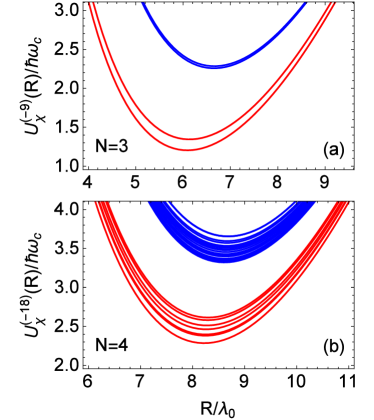
Figure 4: (Color online) Top: Adiabatic potentials $U_{\chi}^{(-9)}(R)$ for $N=3$, $M=-9$ and $\kappa=1$. Bottom: Adiabatic potentials $U_{\chi}^{(-18)}(R)$ for $N=4$, $M=-18$ and $\kappa=1$. Similar to Fig. 3, the larger gaps (on the order of $\hbar\omega_{c}$) indicate magnetic excitations, while the smaller splittings are due to Coulomb interactions. The separate clusters of curves (distinguished by color online) indicate different $K$ manifolds, with $K=|M|$ for the lowest grouping of curves and $K$ increasing from bottom to top.

shows the adiabatic potentials $U_{\chi}^{(M)}(R)$ for $N=3$, $M=-9$, and $\kappa=1$, while Fig 4(b) shows the adiabatic potentials for $N=4$, $M=-18$, and $\kappa=1$. The interactions are weak such that the different K manifolds are still distinguishable. However, the Coulomb interaction has split the degeneracy of the potentials. If $\kappa$ were increased, then the states comprising different $K$ manifolds would begin to overlap.

Without approximations, the many-dimensional Schrödinger equation with Coulomb interactions reduces to an infinite set of one-dimensional coupled ordinary differential equations in terms of the adiabatic potentials:

$$\left\{-\frac{1}{2\mu}\frac{d^{2}}{dR^{2}}+U_{\chi}^{(M)}(R)-E\right\}F_{E\chi}^{(M)}(R)$$

$$-\frac{1}{2\mu}\sum_{\chi^{\prime}}\left\{2P_{\chi\chi^{\prime}}\frac{d}{dR}+Q_{\chi\chi^{\prime}}\right\}F_{E\chi^{\prime}}^{(M)}(R)\ =0.$$ (50)

The $P_{\chi\chi^{\prime}}$ and $Q_{\chi\chi^{\prime}}$ matrices,

$$P_{\chi\chi^{\prime}}(R)=\bigg{\langle}\Phi_{\chi}^{(M)}\bigg{|}\frac{\partial\Phi_{\chi^{\prime}}^{(M)}}{\partial R}\bigg{\rangle}$$ (51)

and

$$Q_{\chi\chi^{\prime}}(R)=\bigg{\langle}\Phi_{\chi}^{(M)}\bigg{|}\frac{\partial^{2}\Phi_{\chi^{\prime}}^{(M)}}{\partial R^{2}}\bigg{\rangle},$$ (52)

describe the non-adiabatic coupling between different channel functions, the $\Phi_{\chi}^{(M)}$.

A good approximation to the adiabatic potentials is to neglect the coupling between different $K$ manifolds and apply degenerate perturbation theory. Diagonalizing the Coulomb matrix in each manifold, with restricted matrix elements $\langle Ka^{\prime}|C(\bm{\Omega})|Ka\rangle$, yields the eigenvalues $C_{K\gamma}^{(M)}$, where the subscript $\gamma$ labels the different eigenstates of the Coulomb matrix in a fixed $K$ manifold. The Coulomb interaction under this approximation reduces the problem to a set of uncoupled one-dimensional potentials, just like in the noninteracting system. The resulting adiabatic potentials are

$$U_{\chi}^{(M)}(R)\approx\delta_{KK^{\prime}}\left(U_{K}^{(M)}(R)+\kappa\frac{C_{K\gamma}^{(M)}}{R}\right).$$ (53)

Fig. 5(a)

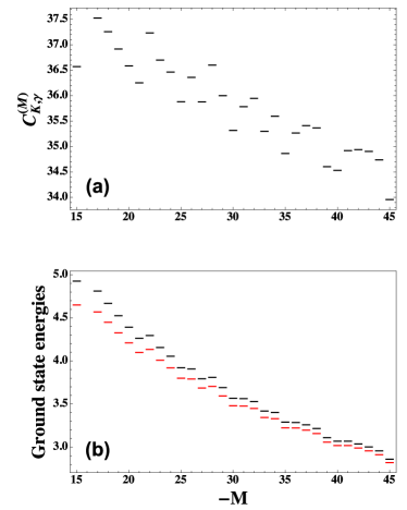
Figure 5: (Color online) (a) The minimum hyperangular Coulomb eigenvalues, the dimensionless $C^{(M)}_{K\gamma}$ in Eq. (53) for $N=6$ particles, obtained by diagonalizing the Coulomb interaction within the degenerate manifolds having $K=-M$ (which corresponds to the lowest Landau level). Coulomb eigenvalues are shown for the $K=15,\ldots,45$ manifolds, which correspond to filling factors $\nu=1\ldots 1/3$. (b) Two Yrast plots, plots of the minimum energy at each $M$, of the $K,M$ manifolds for six particles in the lowest Landau level using different approximations. The energies of the upper (black) curve are calculated entirely in first order perturbation theory in the lowest Landau level. For the lower energies (red), the hyperangular energies are calculated perturbatively (taken from (a) above), but the hyperradial energies are calculated using exact numerical techniques. The lower yrast spectrum constitutes a departure from the strict lowest Landau level approximation. In this model, no confinement potential is included, and particle confinement occurs only due to angular momentum conservation.

shows the lowest hyperangular Coulomb eigenvalues, the $C^{(M)}_{K\gamma}$ , for $N=6$ particles obtained by diagonalizing the Coulomb interaction within the degenerate manifolds having $K=-M$. The minimum eigenvalues are shown from the $K=15$ manifold (filling factor $\nu=1$) to the $K=45$ ($\nu=1/3$). The $C^{(M)}_{K\gamma}$ values shown are dimensionless quantities. A classical minimization of the Coulomb potential at fixed hyperradius gives a lower bound to the quantum eigenvalues, and the following formula gives approximate minimum values, namely:

$$C_{\rm min}(N)\approx(0.12+0.33/N)N^{2}(N-1)$$ (54)

For instance, for $N=6(8)$ particles, the direct minimization gives $C_{\rm min}=31.7824(71.5427)$, whereas the approximate formula gives 31.5 (72.2). The value of $C^{(-45)}_{45,\gamma=1}$ computed with hyperangular wavefunctions is within 7$\%$ of this minimum value. The classical minimum hyperangular Coulomb potential corresponds to the internal geometrical distribution of particles that minimizes the energy for any size system. As $|M|$ is increased, the increasing Hilbert space size allows the particles to better approach this ideal, energy minimizing internal geometry.

Including the potentials of Eq. (53) in Fig. 4 only slightly alters the potentials, and the changes are largest for the higher energy potential curves within a given $K$ manifold. The hyperangular eigenvector corresponding to the smallest eigenvalue is the state that minimizes the Coulomb interactions. For example, we find 98% overlap with the hyperangular numerical ground state and the hyperangular part of the Laughlin function for the three-body system with $K=-M=9$, indicating that the ground state in this system is a quantum liquid. The energies the $K,M$ manifold restricted calculation can be found by multiplying the hyperangular eigenvalues, $C^{(M)}_{K\gamma}$, times the hyperradials energies, which can be found in different ways. Ignoring the changes to the potential curves due to the Coulomb interactions constitutes treating the hyperradial energies to first order in perturbation theory.

Table 1: Comparisons to conventional systems. All rows are estimations of the ground state energy change due to the introduction of the Coulomb interaction,converted to our system of magnetic units, defined in the text. Row 1:Extrapolations of $\Delta E$ from Haldane sphere configuration interaction calculations, using quartic, least squares fits following the method in Ref. Wooten et al. (2013). The extrapolations become less accurate as the computational size of the systems limit the number of different sphere sizes that can be calculated. Row 2: Planar exact numerical diagonalization $\Delta E$ in the lowest Landau level: first two values from Ref. Laughlin (1983b)$*(3/\sqrt{2})$, and last three values from Ref. Gun Sang Jeon (2006). Row 3: Degenerate perturbation theory calculation using hyperspherical picture within a fixed-K manifold along with a first order perturbation treatment of the hyperradial equation. Row 4: Degenerate perturbation theory within the fixed-K manifold with an exact, nonperturbative treatment of the hyperradial differential equation. Row 5: Born-Oppenheimer approximation neglecting nonadiabatic coupling matrices P and Q with exact non-perturbative treatment of the hyperradial differential equation, which constitutes a lower bound approximation when well-converged. Row 6: Adiabatic approximation, which includes the diagonal element of the Q matrix in the lowest potential curve, with an exact, nonperturbative solution of the hyperradial differential equation. These constitute strict upper bounds to the ground state energies.

N,$-M$	3,$9$	3,$15$	4,$18$	5,$30$	6,$45$
$\Delta E$, Haldane sphere, fit, extrapolation	0.71656	0.5526	1.310	2.04	$\approx 3$
$\Delta E$, Planar calculations	0.716527	0.55248	1.30573	2.02725	2.86015
$\Delta E,$ Perturbation Theory	0.716527	0.55248	1.30573	2.02725	2.86015
$\Delta E,$ Degenerate fixed-$K$	0.704637	0.54792	1.28552	1.99742	2.81994
$\Delta E,$ Born-Oppenheimer (lower bound*)	0.70198	0.54722	1.28086	1.99226	–
$\Delta E,$ Adiabatic (upper bound)	0.70204	0.54723	1.28092	1.99230	–

In the lowest Landau level, hyperspherical energy calculations using first order perturbation theory match the results of conventional planar configuration interaction calculations, which are considered the numerical standard in quantum Hall studies. In the hyperspherical treatment, perturbation theory calculations consists of multiplying the hyperangular Coulomb eigenvalues, $C^{(M)}_{K\gamma}$, times the first order perturbation calculations of the hyperradial expectation value of $1/r$ from Eq. 53. The upper (black) Yrast plot in Fig. 4(b) for a six particle hyperspherical system under these approximations is identical to the exact numerical diagonalization plot in Fig.3 of Ref. Gun Sang Jeon (2006) to within the numerical accuracy shown in their Table III Yra . We present a few numerical examples for selected systems in the third row of Table 1. These values are identical to within published numerical accuracy to standard planar numerical calculations Laughlin (1983b); Gun Sang Jeon (2006), given on row 2, and are significantly more accurate than calculations performed using a spherical geometry, given in row 1. Numerical studies in the spherical geometry of Ref. Haldane (1983) are another standard in the quantum Hall system, but while calculations on the Haldane sphere capture much of the physics of the quantum Hall system, they are not considered numerically accurate due to finite size effects. The energy shifts given in row 1 are extrapolations from the spherical geometry to an infinite plane, performed using least squares quartic fits to the energy shifts following Ref. Wooten et al. (2013). Despite the numerical inaccuracy of the spherical geometry, we present these energy shifts as another comparison to standard techniques in the quantum Hall field.

The calculations can be improved from the lowest Landau level restriction by treating the hyperradial energies using exact numerical techniques. In this approximation, we maintain the single $K,M$ manifold degenerate perturbation theory approximation, but consider how the resulting Coulomb hyperangular eigenvalues alter the hyperradial potential curves. Solving the hyperradial Schrödinger equation using exact numerical techniques yields a slightly lower energy than the energies given using pure perturbation theory, as shown in both Fig. 4(b) and row 4 of Table 1. This technique constitutes incorporating additional functional space from higher Landau levels into the Hilbert space of the problem. This approximation would be analogous to a variational energy minimization based on a scaling parameter multiplying all of the single particle radial coordinates from the original Slater determinant basis. The energies are lowered in this approximation because the introduction of Coulomb repulsion expands the hyperradial potential curves outward, and the resulting hyperradial energies are lowered by this expansion. The solutions are still confined by the diamagnetic term of the Hamiltonian, but no additional confinement potential has been included to compress the electrons into a smaller area. Including a confinement potential to model the inward Coulomb pressure due to the bulk might be appropriate in modeling many body condensed matter systems, but it is less appropriate for calculations in trapped atom systems or quantum dots.

More accurate calculations require extending beyond the single $K,M$ manifold approximation, and are not trivial. However, upper and lower bounds on the exact energies of the system can be established using additional approximations. A lower bound can be established using the Born-Oppenheimer approximation Starace and Webster (1979). In this approximation, higher $K$ manifolds with the same $M$ are included in the hyperangular energy calculations, and the hyperradial energies are calculated by solving Eq. IV.5 numerically while neglecting the nonadiabatic coupling $P$ and $Q$ matrices. If the fixed-$R$ hyperangular calculation is fully converged, these values can be proven to be lower bounds on the ground state energies for each of the corresponding symmetries. A few example lower bounds are given in row 5 of Table 1. The upper bounds given shown in row 6 of the same table are calculated under the adiabatic approximation, which differs from the Born-Oppenheimer approximation by including the diagonal elements of the $Q$ matrix in the numerical solution to Eq. IV.5. When fully converged, these values give strict upper bounds to the ground state energy for those symmetries. As before, these upper and lower bounds apply to a system with no additional confining potential besides the diamagnetic confinement.

The fact that the upper and lower bounds in this hyperspherical representation differ by less than $10^{-4}$ for all cases shown is strong evidence that the adiabatic representation is unusually effective in this system. By comparison, the ground state energies of the hydrogen negative ion were found to differ by 1.7% in the corresponding upper and lower bound levels of the approximation, (see Klar and Klar (1978)). A major reason why the adiabatic formulation is much more accurate for the quantum Hall problem is that the charged particles here do not experience any attractive potentials, which cause potential valleys in the H^- system that have much stronger nonadiabaticity.

Another indication that the adiabatic hyperspherical representation is particularly appropriate is that the adiabatic potential curves show only weak nonadiabatic coupling between different manifolds, as evidenced by a relative lack of avoided crossings. The weak coupling between different manifolds makes it difficult to discern any avoided crossings in Fig. 4 on the scale shown. To better visualize any avoided crossings, Fig. 6

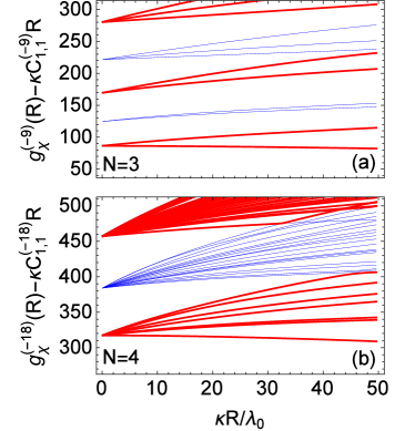
Figure 6: (Color online) Top: $N=3$ scaled adiabatic potentials $g_{\chi}(R)$ [see Eq. (55)] shifted by the smallest eigenvalue $C_{1,1}^{9}$ from diagonalizing the Coulomb interaction in the $K=-M=9$ manifold. Bottom: $N=4$ scaled adiabatic potentials $g_{\chi}(R)$ shifted by the smallest eigenvalue $C_{1,1}^{18}$ from diagonalizing the Coulomb interaction in the $K=|M|=18$ manifold. Alternating thick (red) and thin (blue) lines label different $K$ manifolds.

shows the scaled adiabatic potentials $g_{\chi}^{(M)}(R)$,

$$g_{\chi}^{(M)}(R)=R^{2}\left(U_{\chi}^{(M)}(R)-[(\mu/8)R^{2}+M/2]\right),$$ (55)

for the same three- and four-body systems as in Fig. 4 ($M=-9$ and $M=-18$, respectively, each with $\kappa=1$), though on a much larger scale in $R$. At $R=0$, the system reduces to the eigenvalues of the $\hat{\bm{K}}^{2}$ operator [see Eq. (31)], while at small $R$ the $g_{\chi}(R)$ are linear in $R$ with slopes given by $\kappa C_{K\gamma}^{(M)}$. All of the $C_{K\gamma}^{(M)}$ are positive, so the curves in Fig. 6 have been shifted by the smallest eigenvalue of the lowest $K$ manifold to put the curves within the same scale.

With this scaling, many close avoided crossings become visible through the higher $K$ manifolds. In general, most of the crossings appear diabatic in nature. These crossings occur at much larger hyperradii (here, $\kappa R\gtrsim 50\lambda_{0}$) than the scale of Fig. 4 ($R<11\lambda_{0}$). For comparison, 99% of the noninteracting hyperradial wave function is contained within $R<8.35\lambda_{0}$ for 3 particles and $R<10.25\lambda_{0}$ for 4 particles. Even well outside of this region, the lowest curve of the lowest $K$ manifold remains isolated from the rest, which suggests the adiabatic approximation is a good approximation for the ground state of the lowest Landau level. In addition, although Fig. 6 has $\kappa=1$, the curves are universal, and their behavior changes smoothly with a trivial scaling in $\kappa$. In other words, the excellence of the adiabatic approximation applies within the relevant potential range for a very wide range of magnetic fields.

A quantitative measure of the non-adiabatic coupling strength is the dimensionless quantity $P_{\chi\chi^{\prime}}^{2}(R)/[U_{\chi}^{(M)}(R)-U_{\chi^{\prime}}^{(M)}(R)]$. Figure 7

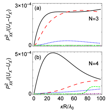
Figure 7: (Color online) $P_{\chi\chi^{\prime}}^{2}(R)/[U_{\chi}^{(M)}(R)-U_{\chi^{\prime}}^{(M)}(R)]$ as a function of $\kappa R$ for $N=3$ and $M=-9$ (top) and $N=4$ and $M=-18$ (bottom) for $\chi=1$. Solid, long-dashed, dotted, dash-dotted, and short-dashed lines are for $\chi^{\prime}=2,3,4,5$ and 6, respectively.

shows this quantity as a function of $\kappa R$ for $N=3$ and $M=-9$, and $N=4$ and $M=-18$ for $\chi=1$ and $\chi^{\prime}=2,\ldots,6$, that is, the five curves represent the coupling strength from the Laughlin 1/3 potential (the lowest channel) to the five next lowest channels. Like the potentials shown in Fig. 6, these curves are also universal in the sense that they scale simply as a function of $\kappa$. Even the strongest nonadiabatic coupling is very small compared to unity, and the coupling to other channels is even weaker still, indicating the validity of the adiabatic approximation. Other higher $\chi^{\prime}$ are not shown as their coupling strength is weaker than ${\cal O}(10^{-5})$.

To conclude this section, the Coulomb interaction acts to split the states within a given $K$ manifold, yet does not lead to strong nonadiabatic coupling within the region where the potentials are deepest. Even with Coulomb interactions, the separation of hyperradial and hyperangular degrees of freedom is an excellent approximation.

V Exceptional degeneracy

One of the benefits in describing this system in hyperspherical coordinates is that the set of antisymmetrized hyperspherical harmonic basis functions in any $K,M$ manifold forms a complete basis in the absence of interactions. From perturbation theory, it is well known that, in a set of functions, turning on interactions will typically act to lower the energy of the ground state relative to all the higher energy states. This effect is strengthened by the presence of additional degeneracy in the system. If the basis functions prior to turning on interactions are degenerate, then increased degeneracy in the noninteracting picture should lead to an increased energy separation of the ground state. In other words, $K,M$ manifolds with enhanced degeneracy relative to their neighboring $K,M^{\prime}$ manifolds should exhibit more strongly gapped ground states. As a result, we predict that manifolds with exceptionally high degeneracy are likely to also be identifiable quantum Hall states.

V.1 Exceptional degeneracy derivation

The following details how the exceptional degeneracy is derived starting from group theory. Only the lowest Landau level is considered in this paper, that is, only those states with $K=-M$.

First, we derive the discrete function of $|M|$ that describes the growth in the number of antisymmetric states. These integer sequences are intimately related to generating functions. For example, from combinatorial considerations, the generating function $G_{N}(x)$ for the overall degeneracy for a fixed $N$ of spin polarized fermions in the lowest Landau level can be derived using integer partitions. In the lowest Landau level, each unsymmetrized $K,M$ manifold of the relative hyperangular functions times $R^{K}$ forms a complete, translationally invariant basis of polynomials in $N=N_{rel}$ variables ($\rho*e^{i\phi}$) that are homogeneous of order $K=|M|$. According to Eq. (25) of Simon et al. (2007), the degeneracy of the symmetric irreducible representation of this basis is equal to

$$d_{sym}(K,N)=p_{N}(K)-p_{N}(K-1),$$ (56)

where $p_{N}(k)$ is the number of partitions of the integer $K$ into parts no longer than $N$. The number of partitions can be calculated using a generating function Olver et al. (2010),

$$Z_{N}(x)=\prod_{j=1}^{N}\frac{1}{1-x^{j}}=\sum_{K=1}^{\infty}x^{K}p_{N}(K).$$ (57)

Combining  (56) and  (57) with the fact that there is a one-to-one mapping between the symmetric irreducible representation at $K$ and the antisymmetric irreducible representation at $K+N(N-1)/2$ yields the generating function

$$G_{N}(x)=x^{N(N-1)/2}\prod_{j=2}^{N}\frac{1}{1-x^{j}}$$ (58)

for spin-polarized fermions in the lowest Landau level. The coefficients of the Taylor sequence of the generating function yields the integer sequence function whose elements $a_{|M|}^{(N)}$ are equal to the number of degenerate antisymmetric states in any given $K=|M|$ manifold. The $a_{|M|}^{(N)}$ coefficients are equivalent to $\overline{\mathcal{N}_{a}}$ defined in section  IV.2. The way this generating function is used is to expand the above product in powers of $x$, namely

$$G_{N}(x)=\sum_{|M|=0}^{\infty}a_{|M|}^{(N)}x^{|M|}.$$ (59)

We have verified by brute force computation that the resulting integer coefficients $a_{|M|}^{(N)}$ are precisely equal to the degeneracy for many values of $N$ and $|M|$. The degeneracies and generating functions can alternately be Yr derived using group theory Curl and Kilpatrick (1960). The points of Fig. 8

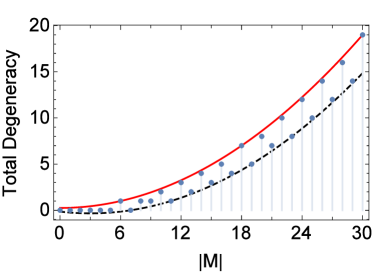
Figure 8: (Color online) Total degeneracy of antisymmetric states for the four-body system in the lowest Landau level as a function of $|M|$. Solid and dashed lines show upper and lower envelope functions, respectively, while the points show the number of degenerate antisymmetric states in that manifold for each value of $|M|=K$.

show the number of antisymmetric states for the four-body system as a function of $|M|$. The first non-zero value at $|M|=6$ is the integer quantum Hall state. There is only the one antisymmetric hyperspherical harmonic function with $K=-M=6$ as is expected for a closed shell in the independent electron picture. Two other notable points on this scale include those at $|M|=18$ and 30, which corresponds to the Laughlin $1/3$ and $1/5$ states, respectively. Otherwise, the general trend as $|M|$ increases is that the number of antisymmetric states oscillates about an overall polynomial growth.

There are many approaches to quantify the small variations in degeneracy on top of this polynomial growth, such as comparing the degeneracy of nearest-neighbors or making comparisons after dividing out the largest power in $|M|$. We choose to derive two polynomial functions that envelop the degeneracies, and then compare the relative heights above the lower envelope. The top envelope function $\bar{a}_{N}^{(M)}$ is forced to go through the integer quantum Hall point at $|M|_{IQH}=N(N-1)/2$, while the bottom function $\underline{a}_{N}^{(M)}$ is forced to go through the zero degeneracy value at $|M|_{IQH}+1$. The solid and dashed lines of Fig. 8 show the upper and lower envelope functions, respectively [see also Eqs. (62) and (63)].

The envelope functions are derived directly from the exact integer sequence degeneracy function $a_{|M|}^{(N)}$. For small systems, Mathematica can usually find the sequence functions directly by using SeriesCoefficient[$G_{N}(x),\{x,0,|M|\}$] ($-M$ is assumed to be non-negative). In our experience, it is easier to first do a partial fraction decomposition of Eq. (58) using Mathematica’s Apart[$G_{N}(x)$], and then find the series coefficient of each term and add them together. Regardless, the sequence function $a_{|M|}^{(N)}$ is grouped in powers of $|M|$. The coefficients of the upper (lower) envelope polynomial are derived by evaluating the coefficients of $a_{|M|}^{(N)}$ at $|M|_{IQH}$ ($|M|_{IQH}+1$).

As a concrete example, for four particles the partial fraction decomposition of $G_{4}(x)$ is

$$G_{4}(x)= \frac{1/24}{(1-x)^{3}}+\frac{-1/8}{(1-x)^{2}}+\frac{23/288}{1-x}+\frac{1/16}{(1+x)^{2}}$$

$$+\frac{-5/32}{1+x}+\frac{-(1-x)}{8(1+x^{2})}+\frac{2+x}{9(1+x+x^{2})}.$$ (60)

Converting Eq. (V.1) to $a_{|M|}^{(4)}$ (using Mathematica functions like ExpToTrig) yields

$$a_{|M|}^{(4)}=\frac{M^{2}}{48}+\frac{(-1)^{|M|}-1}{16}|M|+\frac{1}{288}\bigg{(}\!\!-27(-1)^{|M|}-1$$

$$+36\sin\left(\frac{\pi|M|}{2}\right)-36\cos\left(\frac{\pi|M|}{2}\right)+64\cos\left(\frac{2\pi|M|}{3}\right)\!\!\bigg{)}.$$ (61)

The upper envelope function $\bar{a}_{|M|}^{(4)}$ comes from evaluating the coefficients of Eq. (V.1) at $|M|_{\rm IQH}$. Here $|M|_{\rm IQH}=6$, such that the coefficient of the $|M|^{2}$ term is a constant 1/48 and the coefficient of the $|M|^{1}$ term is 0. The coefficient of the $|M|^{0}$ term is determined last. It is found by forcing the polynomial to equal 1 when evaluated at $|M|_{\rm IQH}$, specifically $36/48+0+x=1$, so a value of $x=1/4$ is the final term. This yields an upper envelope function of

$$\bar{a}_{|M|}^{(4)}=\frac{|M|^{2}}{48}+\frac{1}{4}.$$ (62)

The lower envelope function $\underline{a}_{|M|}^{(4)}$ comes from evaluating the coefficients of Eq. (V.1) at $|M|_{\rm IQH}+1$. Here $|M|_{\rm IQH}+1=7$, such that the coefficient of the $|M|^{2}$ term is a constant 1/48 and the coefficient of the $|M|^{1}$ term is $-1/8$. The coefficient of the $|M|^{0}$ term is determined last. It is found by forcing the polynomial to equal 0 when evaluated at $|M|_{\rm IQH}+1$, specifically $49/48-7/8+x=0$, so a value of $x=-7/48$ is the final term. This yields a lower envelope function of

$$\underline{a}_{|M|}^{(4)}=\frac{|M|^{2}}{48}-\frac{|M|}{8}-\frac{7}{48}.$$ (63)

Defining the upper envelope function as $U_{N}(M)$ and the lower envelope function as $L_{N}(M)$, we have derived the following expressions in terms of the coefficient $C_{N}=N(N-1)/(N!)^{2}$ of the maximum power $|M|^{N-2}$ as:

$$U_{3}/C_{3} =|M|+3$$

$$L_{3}/C_{3} =|M|-4$$

$$U_{4}/C_{4} =M^{2}+12$$

$$L_{4}/C_{4} =M^{2}-6|M|-7$$

$$U_{5}/C_{5} =|M|^{3}-9M^{2}+36|M|+260$$

$$L_{5}/C_{5} =|M|^{3}-9M^{2}-9|M|-143$$

$$U_{6}/C_{6} =M^{4}\!-20|M|^{3}\!+150M^{2}\!-180|M|\!+3105$$

$$L_{6}/C_{6} =M^{4}-20|M|^{3}+60M^{2}+80|M|-256$$

$$U_{7}/C_{7} =|M|^{5}-75M^{4}/2+1340|M|^{3}/3-825M^{2}$$

$$-5865|M|+328293/2$$

$$L_{7}/C_{7} =|M|^{5}-75M^{4}/2+1340|M|^{3}/3-2400M^{2}$$

$$+6560|M|-323576/3$$

$$U_{8}/C_{8} =M^{6}-63|M|^{5}+1400M^{4}-10920|M|^{3}$$

$$-21168M^{2}+784000|M|+5234432$$

$$L_{8}/C_{8} =M^{6}-63|M|^{5}+1400M^{4}-14070|M|^{3}$$

$$+78057M^{2}-552475|M|+714734$$

$$U_{12}/C_{12} =M^{10}-275|M|^{9}+63195M^{8}/2$$

$$-1960200|M|^{7}+70516292M^{6}$$

$$-1440719280|M|^{5}+13562493120M^{4}$$

$$+40317868800|M|^{3}-2246025672000M^{2}$$

$$+20132954569728|M|+289846790411904$$

$$L_{12}/C_{12} =M^{10}-275|M|^{9}+63195M^{8}/2$$

$$-1960200|M|^{7}+70516292M^{6}$$

$$-1460365830|M|^{5}+16263893745M^{4}$$

$$-99340265200|M|^{3}+962578332375M^{2}$$

$$-11917386104239|M|-101761341423733/2$$

From the envelope functions, the relative degeneracy $g_{\rm rel}$ can now be defined as

$$g_{\rm rel}=\frac{a_{|M|}^{(N)}-\underline{a}_{|M|}^{(N)}}{\bar{a}_{|M|}^{(N)}-\underline{a}_{|M|}^{(N)}},$$ (64)

that is, the relative height of $a_{|M|}^{(N)}$ above the lower envelope, with respect to the separation between the two envelope functions.

V.2 Connection between degeneracy and energy gaps

Figure 9

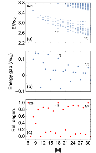
Figure 9: (Color online) Connection between exceptional degeneracy and energy gaps for $N=4$ electrons. (a) The dashes indicate the energies at each $|M|$. The IQH, $1/3$ and $1/5$ filling fractions are labeled. (b) The energy gap is defined as the smallest energy difference between the ground state at $|M|$ and all other states with $|M^{\prime}|\leq|M|$. This could be negative if the comparative state is lower in energy. The IQH state’s energy gap is not shown, but is about $1\hbar\omega_{c}$, since the next nearest state is approximately one vibrational quantum away. (c) The relative degeneracies are defined in Sec. V.1; see specifically Eq. (64).

illustrates the connection between the energy gaps that appear when solving Schrödinger’s equation for different $M$ and the exceptional degeneracies. Panel (a) shows the energies from solving the four-body Schrödinger equation in distinct $K,M$ manifolds for $\kappa=1$ and various $|M|$, but ignoring coupling between $K$ manifolds. The IQH state is recognizable at $|M|=6$ as it is non-degenerate and isolated from the rest. The Laughlin $1/3$ state at $|M|=18$ also shows a significant lowering of the energy compared to neighboring $M$ values. Panel (b) shows the energy gaps, that is, the smallest energy difference between the ground state at $|M|$ and all other states with $|M^{\prime}|\leq|M|$. The IQH state is not shown on this scale as its energy gap is $\approx\hbar\omega_{c}$. Again, the $1/3$ state, among others, shows a prominent positive energy gap. Panel (c) shows the relative degeneracies. The IQH, $1/3$, and $1/5$ states all have unity relative degeneracy, while other states also show prominently. Remarkably, although the upper envelope is derived based only on the IQH state, it passes through all Laughlin-type degeneracy points as well, this precise matching of the upper envelope function does not hold for all higher particle numbers $N$. In general, we designate those $K=-M$ states with relative degeneracy close to one as the exceptionally degenerate states, and suggest that these are candidates for observable $N$-body ground states that are markedly lower in energy than their neighbors.

Figure 10

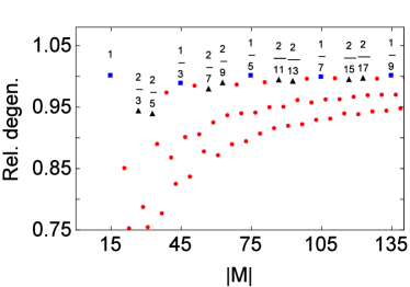
Figure 10: (Color online) Relative degeneracies [see Eq. (64)] for the six-body system are shown as a function of $|M|$. Squares show the integer quantum Hall effect and the Laughlin $\nu=1/3,1/5,\ldots$ states; triangles show the Jain states of two filled composite Landau levels (also called $\Lambda$ levels); circles show the remaining unidentified states.

shows the relative degeneracy as calculated from Eq. (64) for the six-body system as a function of $|M|$. The squares identify the degeneracies in systems with values of $M$ that include the integer quantum hall and Laughlin states. The triangles identify the degeneracies of systems that include the Jain states of two filled composite fermion Landau levels, which also show a large relative degeneracy as compared to their neighbors (which appear near $g_{\rm rel}\approx 0$) and their next-nearest neighbors. Circles show the remaining unidentified states. A brief discussion of the identification of Laughlin and Jain states is given in appendix A.

VI Conclusions

For testably small systems in the lowest Landau level, many of the $K,M$ manifolds of antisymmetrized functions contain the identifiable Laughlin and Jain composite fermion states for few-body systems. The $K,M$ manifolds of the identifiable Laughlin and Jain composite fermion states all exhibit exceptionally high degeneracy compared to the majority of other $K,M$ manifolds in the lowest Landau levels. Although the relative degeneracy does not uniquely identify the known composite fermion filling states, our results suggest that high degeneracy plays a role in strengthening the energy gap of observed and described fractionally filled states. As such, it may also be interesting to examine the low-lying ground states that are associated with exceptionally high relative degeneracy, but which are not associated with the Laughlin or Jain sequences.

The adiabatic hyperspherical potential curves we have calculated are astonishingly devoid of strong couplings and avoided crossings, which is a sign that the adiabatic approximation is extremely and unusually accurate for this system in the parameter range typically probed in FQH experiments. In other words, the hyperradial degree of freedom is accurately quasi-separable in the experimentally studied range of the FQHE. Although the hyperspherical adiabatic approximation in the lowest Landau level reproduces the results of exact numerical configuration interaction calculations, the treatment accesses different aspects of the problem than either the Slater determinant construction or the composite fermion picture. The quasi-separability of the hyperradial degree of freedom is a feature not considered in other treatments of the quantum Hall system, and the hyperradius does not naturally emerge from either the Slater determinant or the composite fermion constructions of the quantum Hall system. At this time, we cannot draw any clear connections between our construction and the composite fermion framework, but suggest that this alternate perspective on the problem may allow us to examine properties of the quantum Hall system that emerge more naturally out of the hyperspherical picture. In particular, the hyperspherical construction suggests the existence of higher energy states that are hyperradial excitations of the ground state wave functions. These hyperradially excited states should have the same internal structure as their ground-state counterparts; excitations between such states should represent a breathing mode that could be probed spectroscopically. These aspects will be explored in future publications.

VII Acknowledgments

We thank Gabor Csathy and Birgit Kaufmann for informative discussions. Critical readings of a preliminary version of this manuscript by Joe Macek and John Quinn are also appreciated.

This work has been supported in part by a Purdue University Research Incentive Grant from the Office of the Vice President for Research. Some numerical calculations were performed under NSF XSEDE Resource Allocation No. TG-PHY150003.

Appendix A Relative $M$ and Identification of Quantum Hall States

Table 2: Sample list of identified N-body quantum Hall states in the lowest Landau level. $M$ is the total relative azimuthal quantum number of Laughlin and Jain states identified by exact numerical diagonalization in a spherical geometry Haldane (1983). $\nu_{CF}$ gives the filling factor of identified QH states according to the Jain composite fermion picture, including a correction that accounts for the finite size shift associated with the spherical geometry. $\nu_{HS}$ is the calculated hyperspherical filling factor, given by Eq.(39). The final column gives a finite size correction to the hyperspherical filling factor.

N	$-M$	$\nu_{CF}$	$\nu_{HS}$	$(\frac{1}{\nu_{CF}}-\frac{1}{\nu_{HS}})$
3	3	1	1	0
	9	$\frac{1}{3}$	$\frac{1}{3}$	$0$
	15	$\frac{1}{5}$	$\frac{1}{5}$	$0$
4	6	1	1	0
	12	$\frac{2}{5}$	$\frac{1}{2}$	$-\frac{1}{2}$
	18	$\frac{1}{3}$	$\frac{1}{3}$	$0$
	24	$\frac{2}{7}$	$\frac{1}{4}$	$-\frac{1}{2}$
	30	$\frac{1}{5}$	$\frac{1}{5}$	$0$
6	15	1	1	0
	27	$\frac{2}{3}$	$\frac{5}{9}$	$-\frac{3}{10}$
	33	$\frac{2}{5}$	$\frac{5}{11}$	$\frac{3}{10}$
	45	$\frac{1}{3}$	$\frac{1}{3}$	$0$
	57	$\frac{2}{7}$	$\frac{5}{19}$	$-\frac{3}{10}$
	75	$\frac{1}{5}$	$\frac{1}{5}$	$0$

Table 3: Jain Composite Fermion states in the lowest Landau level. The $M$ for an $N$-particle system at filling fraction $\nu=\nu^{*}/(1+2p\nu^{*})$ are given for the composite fermion states most strongly observed in experiments, where $p$ is an integer indicating the number of pairs of composite fermion flux tubes attached to each electron.

$\nu^{*}$	$-M$	Restrictions
1	$\frac{N(N-1)}{2}(2p+1)$
2	$N(\frac{N-4}{4}+p(N-1))$	even N only
-2	$N(-\frac{N-4}{4}+p(N-1))$	even N only
3	$N(\frac{N-9}{6}+p(N-1))$	$N\bmod{3}=0$ only
-3	$N(-\frac{N-9}{6}+p(N-1))$	$N\bmod{3}=0$ only

The identification of the experimentally observed fractional quantum Hall states in systems with a modest number of particles is not trivial. Although the high exceptional degeneracy of a $K,|M|$ manifold is highly correlated with the presence of a quantum Hall ground state, it is not demonstrated to be a diagnostic of the presence of a quantum Hall state. In addition, the filling fraction as given by Eq. (35) is correct in the thermodynamic limit but is only approximately correct for small systems. It is also of limited use for uniquely identifying the quantum Hall ground states. Instead, the fractional quantum Hall states of important filling factors are identified by using results from conventional, exact numerical diagonalizations in finite systems using planar, spherical, or toroidal geometry.

For example, in a system of 6 particles, Eq. (35) would predict that the $\nu=1/3$ state should appear when the single particle Hilbert space is restricted to 18 orbitals in the lowest Landau level, or, in other words, when the number of magnetic flux quanta in the system, $N_{\phi}=BA/\phi_{0}$, is 18. This would correspond to a planar system with $m$ restricted to $m_{i}=0,-1,\ldots,-17$. However, traditional numerical diagonalization identify the highly-gapped $\nu=1/3$ state in a slightly smaller system where $N_{\phi}=16$ and $m_{i}=0,-1,\ldots,-15$. The numerical ground state is a state with $M=-45$ and exhibits the signature of a quantum Hall state in numerical trials: a non-degenerate, translation and rotation invariant ground state with a strong energy gap. This numerical ground state is nearly identical to the famous Laughlin ansatz wave function for many different numbers of particles Laughlin (1983a, c); Fano et al. (1986); Prange and Girvin (1987) and has been identified as the ground state of the $\nu=1/3$ system.

The small correction to the filling factor calculated using Eq. (35) is due to the finite size of the system, and the uncorrected filling factor approaches the ideal rational fractions of the experimental system in the thermodynamic limit. The precise locations of many quantum Hall states have been established in numerical trials for a wide variety of states. The $M$ of the Laughlin filling functions ($\nu=1/m$ for $m=$ odd integers) are easy to establish based on the form of the Laughlin wave function. For a system with $N$ particles, the Laughlin $1/m$ wave function on the plane always occurs at $M=-mN(N-1)/2$. The relative azimuthal angular momentum, $M$, of in the independent particle picture is always a good quantum number, and is the same as the $M$ of the hyperspherical picture. As a result, we use the conventional system to identify which $M$ manifolds in the hyperspherical system contain the previously identified quantum Hall states.

The locations of the Jain composite fermion states on the plane (e.g. $\nu=2/5,3/7,etc\ldots$) were established by using the Jain composite fermion picture Jain (1989, 2007). The composite fermion sequence is found for choices of $\nu^{*}=1,\pm 2,\pm 3,\ldots$ and positive integer $p$ at the filling factors $\nu$ given by

$$\nu=\frac{\nu^{*}}{1+2p\nu^{*}}.$$ (65)

The strongest composite fermion states correspond to smaller values of $|\nu^{*}|$ and $p$. We have used the composite fermion construction on the Haldane sphere Haldane (1983) to identify the planar $M$ values for the Jain states. Because these electronic wave functions on the sphere involve only single-particle wave functions in the lowest Landau level, they can be mapped straightforwardly from the Haldane sphere to the infinite plane according to a stereographic mapping Fano et al. (1986). The planar $M$ values for the strongest quantum Hall states for three, four, and six particles are shown in Table 2. The filling fractions of the composite fermion picture ($\nu_{CF}$) are corrected to their values in the thermodynamic limit. For a more general system, the values of $M$ for the strongest composite fermion states can be calculated according to Table 3. Other hyperspherical filling factors cannot be matched to a filling factor in the thermodynamic limit in the absence of either a theoretical picture (i.e. CF theory) or a series of numerical trials with many more particles that would allow the unidentified states to be extrapolated to be extrapolated to the many-particle case.

References

- Tsui et al. (1982) D. C. Tsui, H. L. Stormer, and A. C. Gossard, Phys. Rev. Lett. 48, 1559 (1982).
- Stormer et al. (1999) H. L. Stormer, D. C. Tsui, and A. C. Gossard, Rev. Mod. Phys. 71, S298 (1999).
- Laughlin (1983a) R. B. Laughlin, Phys. Rev. Lett. 50, 1395 (1983a).
- Jain (1989) J. K. Jain, Phys. Rev. Lett. 63, 199 (1989).
- Jain (2007) J. K. Jain, Composite Fermions (Cambridge University Press, United Kingdom, 2007).
- Haldane (1983) F. D. M. Haldane, Phys. Rev. Lett. 51, 605 (1983).
- Halperin (1984) B. I. Halperin, Phys. Rev. Lett. 52, 1583 (1984).
- Moore and Read (1991) G. Moore and N. Read, Nuclear Physics B 360, 362 (1991).
- Ginocchio and Haxton (1996) J. N. Ginocchio and W. C. Haxton, Phys. Rev. Lett. 77, 1568 (1996).
- Wójs et al. (2004) A. Wójs, K.-S. Yi, and J. J. Quinn, Phys. Rev. B 69, 205322 (2004).
- Haldane and Rezayi (1985) F. D. M. Haldane and E. H. Rezayi, Phys. Rev. Lett. 54, 237 (1985).
- Jeon et al. (2007) G. S. Jeon, C.-C. Chang, and J. K. Jain, The European Physical Journal B 55, 271 (2007), ISSN 1434-6028.
- Mukherjee et al. (2014) S. Mukherjee, S. S. Mandal, Y.-H. Wu, A. Wójs, and J. K. Jain, Phys. Rev. Lett. 112, 016801 (2014).
- Macek (1968) J. Macek, J. Phys. B 1, 831 (1968).
- Fano (1981) U. Fano, Phys. Rev. A 24, 2402 (1981).
- Fano (1983) U. Fano, Phys. Rev. A 27, 1208 (1983).
- Smirnov and Shitikova (1977) Y. F. Smirnov and K. V. Shitikova, Sov. J. Part. Nucl. 8, 44 (1977).
- Avery (1989) J. Avery, Hyperspherical Harmonics: Applications in Quantum Theory (Kluwer Academic Publishers, Norwell, MA, 1989).
- Avery (1993) J. Avery, J. Phys. Chem. 97, 2406 (1993).
- Nielsen et al. (2001) E. Nielsen, D. V. Fedorov, A. S. Jensen, and E. Garrido, Phys. Rep. 347, 373 (2001).
- Daily et al. (2015a) K. M. Daily, A. Kievsky, and C. H. Greene, arxiv (2015a), 1503.05978.
- Wang et al. (2013) Y. Wang, J. P. D’Incao, and B. D. Esry, in Adv. At. Mol. Opt. Phys., edited by P. R. B. Ennio Arimondo and C. C. Lin (Academic Press, 2013), vol. 62, pp. 1 – 115.
- Rittenhouse et al. (2011) S. T. Rittenhouse, J. von Stecher, J. P. D’Incao, N. P. Mehta, and C. H. Greene, Journal of Physics B: Atomic, Molecular and Optical Physics 44, 172001 (2011).
- Wang et al. (2014) Y. Wang, P. S. Julienne, and C. H. Greene, arxiv (2014), 1412.8094.
- Efimov (1970) V. Efimov, Phys. Lett. B 33, 563 (1970).
- Nielsen and Macek (1999) E. Nielsen and J. H. Macek, Phys. Rev. Lett. 83, 1566 (1999).
- Gattobigio et al. (2012) M. Gattobigio, A. Kievsky, and M. Viviani, Phys. Rev. A 86, 042513 (2012).
- Lin (1986) C. D. Lin, Adv. At. Mol. Opt. Phys. 22, 77 (1986).
- Lin (1995) C. D. Lin, Phys. Rep. 257, 1 (1995).
- Lin and Morishita (2000) C. D. Lin and T. Morishita, Phys. Essays 13, 367 (2000).
- Botero and Greene (1985) J. Botero and C. H. Greene, Phys. Rev. A 32, 1249 (1985).
- Daily and Greene (2014) K. M. Daily and C. H. Greene, Phys. Rev. A 89, 012503 (2014).
- Daily et al. (2015b) K. M. Daily, J. von Stecher, and C. H. Greene, Phys. Rev. A 91, 012512 (2015b).
- Archer et al. (1990) B. J. Archer, G. A. Parker, and R. T. Pack, Phys. Rev. A 41, 1303 (1990).
- Bohn et al. (1998) J. L. Bohn, B. D. Esry, and C. H. Greene, Phys. Rev. A 58, 584 (1998).
- Kushibe et al. (2004) D. Kushibe, M. Mutou, T. Morishita, S. Watanabe, and M. Matsuzawa, Phys. Rev. A 70, 063617 (2004).
- Rittenhouse et al. (2006) S. T. Rittenhouse, M. J. Cavagnero, J. von Stecher, and C. H. Greene, Phys. Rev. A 74, 053624 (2006).
- Efros (1995) V. D. Efros, Few-Body Systems 19, 167 (1995).
- Delves (1959) L. M. Delves, Nucl. Phys. 9, 391 (1959).
- Delves (1960) L. M. Delves, Nucl. Phys. 20, 275 (1960).
- Barnea (1999) N. Barnea, Phys. Rev. A 59, 1135 (1999).
- Krivec (1998) R. Krivec, Few-Body Systems 25, 199 (1998), ISSN 0177-7963.
- Viviani (1998) M. Viviani, Few-Body Systems 25, 177 (1998).
- Pan et al. (2008) W. Pan, J. S. Xia, H. L. Stormer, D. C. Tsui, C. Vicente, E. D. Adams, N. S. Sullivan, L. N. Pfeiffer, K. W. Baldwin, and K. W. West, Phys. Rev. B 77, 075307 (2008).
- Eisenstein and Stormer (1990) J. P. Eisenstein and H. L. Stormer, Science 248, pp. 1510 (1990).
- Wooten et al. (2013) R. E. Wooten, J. H. Macek, and J. J. Quinn, Phys. Rev. B 88, 155421 (2013).
- Laughlin (1983b) R. B. Laughlin, Phys. Rev. B 27, 3383 (1983b).
- Gun Sang Jeon (2006) J. K. J. Gun Sang Jeon, Chia-Chen Chang (2006), eprint cond-mat/0611309.
- (49) The exceptions occur at , where in Gun Sang Jeon (2006), the given energies are repeated from , respectively. In our numerical studies, these are the cases where the energy has increased with increasing . The discrepancies between our tables occur because Table III gives the lowest energy as a function of total (including the center of mass), rather than as a function of relative , as in our calculations.
- Starace and Webster (1979) A. F. Starace and G. L. Webster, Phys. Rev. A 19, 1629 (1979).
- Klar and Klar (1978) H. Klar and M. Klar, Phys. Rev. A 17, 1007 (1978).
- Simon et al. (2007) S. H. Simon, E. H. Rezayi, and N. R. Cooper, Phys. Rev. B 75, 195306 (2007).
- Olver et al. (2010) F. W. Olver, D. W. Lozier, R. F. Boisvert, and C. W. Clark, NIST Handbook of Mathematical Functions (Cambridge University Press, New York, NY, USA, 2010), 1st ed.
- Curl and Kilpatrick (1960) R. F. Curl and J. E. Kilpatrick, American Journal of Physics 28, 357 (1960).
- Laughlin (1983c) R. B. Laughlin, Phys. Rev. B 27, 3383 (1983c).
- Fano et al. (1986) G. Fano, F. Ortolani, and E. Colombo, Phys. Rev. B 34, 2670 (1986).
- Prange and Girvin (1987) R. E. Prange and S. M. Girvin, The Quantum Hall Effect (Springer-Verlag, New York, 1987).