Global Constraint for Sequential Pattern Mining

Prefix-Projection Global Constraint for Sequential Pattern Mining

Abstract

Sequential pattern mining under constraints is a challenging data mining task. Many efficient ad hoc methods have been developed for mining sequential patterns, but they are all suffering from a lack of genericity. Recent works have investigated Constraint Programming (CP) methods, but they are not still effective because of their encoding. In this paper, we propose a global constraint based on the projected databases principle which remedies to this drawback. Experiments show that our approach clearly outperforms CP approaches and competes well with ad hoc methods on large datasets.

1 Introduction

Mining useful patterns in sequential data is a challenging task. Sequential pattern mining is among the most important and popular data mining task with many real applications such as the analysis of web click-streams, medical or biological data and textual data. For effectiveness and efficiency considerations, many authors have promoted the use of constraints to focus on the most promising patterns according to the interests given by the final user. In line with [15], many efficient ad hoc methods have been developed but they suffer from a lack of genericity to handle and to push simultaneously sophisticated combination of various types of constraints. Indeed, new constraints have to be hand-coded and their combinations often require new implementations.

Recently, several proposals have investigated relationships between sequential pattern mining and constraint programming (CP) to revisit data mining tasks in a declarative and generic way [5, 11, 9, 12]. The great advantage of these approaches is their flexibility. The user can model a problem and express his queries by specifying what constraints need to be satisfied. But, all these proposals are not effective enough because of their CP encoding. Consequently, the design of new efficient declarative models for mining useful patterns in sequential data is clearly an important challenge for CP.

To address this challenge, we investigate in this paper the other side of the cross fertilization between data-mining and constraint programming, namely how the CP framework can benefit from the power of candidate pruning mechanisms used in sequential pattern mining. First, we introduce the global constraint Prefix-Projection for sequential pattern mining. Prefix-Projection uses a concise encoding and its filtering relies on the principle of projected databases [14]. The key idea is to divide the initial database into smaller ones projected on the frequent subsequences obtained so far, then, mine locally frequent patterns in each projected database by growing a frequent prefix. This global constraint utilizes the principle of prefix-projected database to keep only locally frequent items alongside projected databases in order to remove infrequent ones from the domains of variables. Second, we show how the concise encoding allows for a straightforward implementation of the frequency constraint (Prefix-Projection constraint) and constraints on patterns such as size, item membership and regular expressions and the simultaneous combination of them. Finally, experiments show that our approach clearly outperforms CP approaches and competes well with ad hoc methods on large datasets for mining frequent sequential patterns or patterns under various constraints. It is worth noting that the experiments show that our approach achieves scalability while it is a major issue of CP approaches.

The paper is organized as follows. Section 2 recalls preliminaries. Section 3 provides a critical review of ad hoc methods and CP approaches for sequential pattern mining. Section 4 presents the global constraint Prefix-Projection. Section 5 reports experiments we performed. Finally, we conclude and draw some perspectives.

2 Preliminaries

This section presents background knowledge about sequential pattern mining and constraint satisfaction problems.

2.1 Sequential Patterns

Let $\mathcal{I}$ be a finite set of items. The language of sequences corresponds to $\mathcal{L_{I}}=\mathcal{I}^{n}$ where $n\in\mbox{$\mathbb{N}$}^{+}$.

Definition 1 (sequence, sequence database)

A sequence $s$ over $\mathcal{L_{I}}$ is an ordered list $\langle s_{1}s_{2}\ldots s_{n}\rangle$, where $s_{i}$, $1\leq i\leq n$, is an item. $n$ is called the length of the sequence $s$. A sequence database $SDB$ is a set of tuples $(sid,s)$, where $sid$ is a sequence identifier and $s$ a sequence.

Definition 2 (subsequence, $\preceq$ relation)

A sequence $\alpha=\langle\alpha_{1}\ldots\alpha_{m}\rangle$ is a subsequence of $s=\langle s_{1}\ldots s_{n}\rangle$, denoted by ($\alpha$ $\preceq$ $s$), if $m\leq n$ and there exist integers $1\leq j_{1}\leq\ldots\leq j_{m}\leq n$, such that $\alpha_{i}=s_{j_{i}}$ for all $1\leq i\leq m$. We also say that $\alpha$ is contained in $s$ or $s$ is a super-sequence of $\alpha$. For example, the sequence $\langle BABC\rangle$ is a super-sequence of $\langle AC\rangle$ : $\langle AC\rangle$ $\preceq$ $\langle BABC\rangle$. A tuple $(sid,s)$ contains a sequence $\alpha$, if $\alpha$ $\preceq$ $s$.

The cover of a sequence $p$ in $SDB$ is the set of all tuples in $SDB$ in which $p$ is contained. The support of a sequence $p$ in $SDB$ is the number of tuples in $SDB$ which contain $p$.

Definition 3 (coverage, support)

Let $SDB$ be a sequence database and $p$ a sequence. $cover_{SDB}(p)$$=$$\{(sid,s)\in SDB\,|\,p\,\mbox{$\preceq$}\,s\}$ and $sup_{SDB}(p)=\#cover_{SDB}(p)$.

Definition 4 (sequential pattern)

Given a minimum support threshold $minsup$, every sequence $p$ such that $sup_{SDB}(p)\geq minsup$ is called a sequential pattern [1]. $p$ is said to be frequent in $SDB$.

sid	Sequence
$1$	$\langle ABCBC\rangle$
$2$	$\langle BABC\rangle$
$3$	$\langle AB\rangle$
$4$	$\langle BCD\rangle$

Table 1: $SDB_{1}$: a sequence database example.

Example 1

Table 1 represents a sequence database of four sequences where the set of items is $\mathcal{I}=\{A,B,C,D\}$. Let the sequence $p={{\mbox{$\langle AC\rangle$}}}$. We have $cover_{{SDB}1}(p)=\{(1,s_{1}),(2,s_{2})\}$. If we consider $minsup=2$, $p={{\mbox{$\langle AC\rangle$}}}$ is a sequential pattern because $sup_{SDB_{1}}(p)\geq 2$.

Definition 5 (sequential pattern mining (SPM))

Given a sequence database $SDB$ and a minimum support threshold $minsup$. The problem of sequential pattern mining is to find all patterns $p$ such that $sup_{SDB}(p)\geq minsup$.

2.2 SPM under Constraints

In this section, we define the problem of mining sequential patterns in a sequence database satisfying user-defined constraints Then, we review the most usual constraints for the sequential mining problem [15].

Problem statement. Given a constraint $C(p)$ on pattern $p$ and a sequence database SDB, the problem of constraint-based pattern mining is to find the complete set of patterns satisfying $C(p)$. In the following, we present different types of constraints that we explicit in the context of sequence mining. All these constraints will be handled by our concise encoding (see Sections 4.2 and 4.5).

- The minimum size constraint $size(p,\ell_{min})$ states that the number of items of $p$ must be greater than or equal to $\ell_{min}$.

- The item constraint $item(p,t)$ states that an item $t$ must belong (or not) to a pattern $p$.

- The regular expression constraint [7] $reg(p,exp)$ states that a pattern $p$ must be accepted by the deterministic finite automata associated to the regular expression $exp$.

2.3 Projected Databases

We now present the necessary definitions related to the concept of projected databases [14].

Definition 6 (prefix, projection, suffix)

Let $\beta={{\mbox{$\langle\beta_{1}\ldots\beta_{n}\rangle$}}}$ and $\alpha={{\mbox{$\langle\alpha_{1}\ldots\alpha_{m}\rangle$}}}$ be two sequences, where $m\leq n$.
- Sequence $\alpha$ is called the prefix of $\beta$ iff $\forall i\in[1..m],\alpha_{i}=\beta_{i}$.
- Sequence $\beta={{\mbox{$\langle\beta_{1}\ldots\beta_{n}\rangle$}}}$ is called the projection of some sequence $s$ w.r.t. $\alpha$, iff (1) $\beta\,\mbox{$\preceq$}\,s$, (2) $\alpha$ is a prefix of $\beta$ and (3) there exists no proper super-sequence $\beta^{\prime}$ of $\beta$ such that $\beta^{\prime}\,\mbox{$\preceq$}\,s$ and $\beta^{\prime}$ also has $\alpha$ as prefix.
- Sequence $\gamma={{\mbox{$\langle\beta_{m+1}\ldots\beta_{n}\rangle$}}}$ is called the suffix of $s$ w.r.t. $\alpha$. With the standard concatenation operator "$concat$", we have $\beta=concat(\alpha,\gamma)$.

Definition 7 (projected database)

Let $SDB$ be a sequence database, the $\alpha$-projected database, denoted by $SDB|_{\alpha}$, is the collection of suffixes of sequences in $SDB$ w.r.t. prefix $\alpha$.

[14] have proposed an efficient algorithm, called PrefixSpan, for mining sequential patterns based on the concept of projected databases. It proceeds by dividing the initial database into smaller ones projected on the frequent subsequences obtained so far; only their corresponding suffixes are kept. Then, sequential patterns are mined in each projected database by exploring only locally frequent patterns.

Example 2

Let us consider the sequence database of Table 1 with $minsup=2$. PrefixSpan starts by scanning ${SDB}_{1}$ to find all the frequent items, each of them is used as a prefix to get projected databases. For ${SDB}_{1}$, we get $3$ disjoint subsets w.r.t. the prefixes $\langle A\rangle$, $\langle B\rangle$, and $\langle C\rangle$. For instance, ${SDB}_{1}|_{{{\mbox{$\langle A\rangle$}}}}$ consists of 3 suffix sequences: $\{(1,{{\mbox{$\langle BCBC\rangle$}}})$, $(2,{{\mbox{$\langle BC\rangle$}}})$, $(3,{{\mbox{$\langle B\rangle$}}})\}$. Consider the projected database ${SDB}_{1}|_{<A>}$, its locally frequent items are $B$ and $C$. Thus, ${SDB}_{1}|_{<A>}$ can be recursively partitioned into 2 subsets w.r.t. the two prefixes $\langle AB\rangle$ and $\langle AC\rangle$. The $\langle AB\rangle$- and $\langle AC\rangle$- projected databases can be constructed and recursively mined similarly. The processing of a $\alpha$-projected database terminates when no frequent subsequence can be generated.

Proposition 1 establishes the support count of a sequence $\gamma$ in $SDB|_{\alpha}$ [14]:

Proposition 1 (Support count)

For any sequence $\gamma$ in $SDB$ with prefix $\alpha$ and suffix $\beta$ s.t. $\gamma=concat(\alpha,\beta$), $sup_{SDB}(\gamma)=sup_{SDB|_{\alpha}}(\beta)$.

This proposition ensures that only the sequences in $SDB$ grown from $\alpha$ need to be considered for the support count of a sequence $\gamma$. Furthermore, only those suffixes with prefix $\alpha$ should be counted.

2.4 CSP and Global Constraints

A Constraint Satisfaction Problem (CSP) consists of a set $X$ of $n$ variables, a domain $\mathcal{D}$ mapping each variable $X_{i}\in X$ to a finite set of values $D(X_{i})$, and a set of constraints $\mathcal{C}$. An assignment $\sigma$ is a mapping from variables in $X$ to values in their domains: $\forall X_{i}\in X,\sigma(X_{i})\in D(X_{i})$. A constraint $c\in\mathcal{C}$ is a subset of the cartesian product of the domains of the variables that are in $c$. The goal is to find an assignment such that all constraints are satisfied.

Domain consistency (DC). Constraint solvers typically use backtracking search to explore the space of partial assignments. At each assignment, filtering algorithms prune the search space by enforcing local consistency properties like domain consistency. A constraint $c$ on $X$ is domain consistent, if and only if, for every $X_{i}\in X$ and for every $d_{i}\in D(X_{i})$, there is an assignment $\sigma$ satisfying $c$ such that $\sigma(X_{i})=d_{i}$. Such an assignment is called a support.

Global constraints provide shorthands to often-used combinatorial substructures. We present two global constraints. Let $X={{\mbox{$\langle X_{1},X_{2},...,X_{n}\rangle$}}}$ be a sequence of $n$ variables.

Let $V$ be a set of values, $l$ and $u$ be two integers s.t. $0\leq l\leq u\leq n$, the constraint Among$(X,V,l,u)$ states that each value $a\in V$ should occur at least $l$ times and at most $u$ times in $X$ [4]. Given a deterministic finite automaton $A$, the constraint Regular$(X,A)$ ensures that the sequence $X$ is accepted by $A$ [16].

3 Related works

This section provides a critical review of ad hoc methods and CP approaches for SPM.

3.1 Ad hoc Methods for SPM

GSP [17] was the first algorithm proposed to extract sequential patterns. It uses a generate-and test approach. Later, two major classes of methods have been proposed:

- Depth-first search based on a vertical database format e.g. cSpade incorporating contraints (max-gap, max-span, length) [21], SPADE [22] or SPAM [2].

- Projected pattern growth such as PrefixSpan [14] and its extensions, e.g. CloSpan for mining closed sequential patterns [19] or Gap-BIDE [10] tackling the gap constraint.

In [7], the authors proposed SPIRIT based on GSP for SPM with regular expressions. Later, [18] introduces Sequence Mining Automata (SMA), a new approach based on a specialized kind of Petri Net. Two variants of SMA were proposed: SMA-1P (SMA one pass) and SMA-FC (SMA Full Check). SMA-1P processes by means of the SMA all sequences one by one, and enters all resulting valid patterns in a hash table for support counting, while SMA-FC allows frequency based pruning during the scan of the database. Finally, [15] provides a survey for other constraints such as regular expressions, length and aggregates. But, all these proposals, though efficient, are ad hoc methods suffering from a lack of genericity. Adding new constraints often requires to develop new implementations.

3.2 CP Methods for SPM

Following the work of [8] for itemset mining, several methods have been proposed to mine sequential patterns using CP.

Proposals. [5] have proposed a first SAT-based model for discovering a special class of patterns with wildcards in a single sequence under different types of constraints (e.g. frequency, maximality, closedness). [11] have proposed a CSP model for SPM. Each sequence is encoded by an automaton capturing all subsequences that can occur in it. [9] have proposed a CSP model for SPM with wildcards. They show how some constraints dealing with local patterns (e.g. frequency, size, gap, regular expressions) and constraints defining more complex patterns such as relevant subgroups [13] and top-$k$ patterns can be modeled using a CSP. [12] have proposed two CP encodings for the SPM. The first one uses a global constraint to encode the subsequence relation (denoted global-p.f), while the second one encodes explicitly this relation using additional variables and constraints (denoted decomposed-p.f).

All these proposals use reified constraints to encode the database. A reified constraint associates a boolean variable to a constraint reflecting whether the constraint is satisfied (value 1) or not (value 0). For each sequence $s$ of $SDB$, a reified constraint, stating whether (or not) the unknown pattern $p$ is a subsequence of $s$, is imposed: $(S_{s}=1)\Leftrightarrow(p\preceq s)$. A great consequence is that the encoding of the frequency measure is straightforward: $freq(p)=\sum_{s\in SDB}S_{s}$. But such an encoding has a major drawback since it requires $(m=\#SDB)$ reified constraints to encode the whole database. This constitutes a strong limitation of the size of the databases that could be managed.

Most of these proposals encode the subsequence relation $(p\preceq s)$ using variables $Pos_{s,j}$ $(s\in SDB$ and $1\leq j\leq\ell)$ to determine a position where $p$ occurs in $s$. Such an encoding requires a large number of additional variables ($m$$\times$$\ell$) and makes the labeling computationally expensive. In order to address this drawback, [12] have proposed a global constraint exists-embedding to encode the subsequence relation, and used projected frequency within an ad hoc specific branching strategy to keep only frequent items before branching over the variables of the pattern. But, this encoding still relies on reified constraints and requires to impose $m$ exists-embedding global constraints.

So, we propose in the next section the Prefix-Projection global constraint that fully exploits the principle of projected databases to encode both the subsequence relation and the frequency constraint. Prefix-Projection does not require any reified constraints nor any extra variables to encode the subsequence relation. As a consequence, usual SPM constraints (see Section 2.2) can be encoded in a straightforward way using directly the (global) constraints of the CP solver.

4 Prefix-Projection Global Constraint

This section presents the Prefix-Projection global constraint for the SPM problem.

4.1 A Concise Encoding

Let $P$ be the unknown pattern of size $\ell$ we are looking for. The symbol $\Box$ stands for an empty item and denotes the end of a sequence. The unknown pattern $P$ is encoded with a sequence of $\ell$ variables $\langle P_{1},P_{2},\ldots,P_{\ell}\rangle$ s.t. $\forall i\in[1\ldots\ell],D(P_{i})=\mathcal{I}\cup\{\mbox{$\Box$}\}$. There are two basic rules on the domains:

1. To avoid the empty sequence, the first item of $P$ must be non empty, so $(\mbox{$\Box$}\not\in D_{1})$.

2. To allow patterns with less than $\ell$ items, we impose that $\forall i\in[1..(\ell$$-$$1)],(P_{i}=\mbox{$\Box$})\rightarrow(P_{i+1}=\mbox{$\Box$})$.

4.2 Definition and Consistency Checking

The global constraint Prefix-Projection ensures both subsequence relation and minimum frequency constraint.

Definition 8 (Prefix-Projection global constraint)

Let $P={{\mbox{$\langle P_{1},P_{2},\ldots,P_{\ell}\rangle$}}}$ be a pattern of size $\ell$. ${{\mbox{$\langle d_{1},...,d_{\ell}\rangle$}}}\in D(P_{1})\times\ldots\times D(P_{\ell})$ is a solution of Prefix-Projection $(P,SDB,minsup)$ iff $sup_{SDB}({{\mbox{$\langle d_{1},...,d_{\ell}\rangle$}}})\geq minsup$.

Proposition 2

A Prefix-Projection $(P,SDB,minsup)$ constraint has a solution if and only if there exists an assignment $\sigma={{\mbox{$\langle d_{1},...,d_{\ell}\rangle$}}}$ of variables of $P$ s.t. $SDB|_{\sigma}$ has at least $minsup$ suffixes of $\sigma$: $\#SDB|_{\sigma}\geq minsup$.

Proof: This is a direct consequence of proposition 1. We have straightforwardly $sup_{SDB}(\sigma)=sup_{SDB|_{\sigma}}({{\mbox{$\langle\rangle$}}})=\#SDB|_{\sigma}$. Thus, suffixes of $SDB|_{\sigma}$ are supports of $\sigma$ in the constraint Prefix-Projection $(P,SDB,minsup)$, provided that $\#SDB|_{\sigma}\geq minsup$. $\Box$

The following proposition characterizes values in the domain of unassigned (i.e. future) variable $P_{i+1}$ that are consistent with the current assignment of variables $\langle P_{1},...,P_{i}\rangle$.

Proposition 3

Let $\sigma={{\mbox{$\langle d_{1},\dots,d_{i}\rangle$}}}$ be a current assignment of variables $\langle P_{1},\dots,P_{i}\rangle$, $P_{i+1}$ be a future variable. A value $d\in D(P_{i+1})$ appears in a solution for Prefix-Projection $(P,SDB,minsup)$ if and only if $d$ is a frequent item in $SDB|_{\sigma}$:

$$\#\{(sid,\gamma)|(sid,\gamma)\in SDB|_{\sigma}\wedge{{\mbox{$\langle d\rangle$}}}\mbox{$\preceq$}\gamma\}\geq minsup$$

Proof: Suppose that value $d\in D(P_{i+1})$ occurs in $SDB|_{\sigma}$ more than $minsup$. From proposition 1, we have $sup_{SDB}(concat(\sigma,{{\mbox{$\langle d\rangle$}}}))=sup_{SDB|_{\sigma}}({{\mbox{$\langle d\rangle$}}})$. Hence, the assignment $\sigma\cup{{\mbox{$\langle d\rangle$}}}$ satisfies the constraint, so $d\in D(P_{i+1})$ participates in a solution. $\Box$

Anti-monotonicity of the frequency measure. If a pattern $p$ is not frequent, then any pattern $p^{\prime}$ satisfying $p\,\mbox{$\preceq$}\,p^{\prime}$ is not frequent. From proposition 3 and according to the anti-monotonicity property, we can derive the following pruning rule:

Proposition 4

Let $\sigma={{\mbox{$\langle d_{1},\dots,d_{i}\rangle$}}}$ be a current assignment of variables $\langle P_{1},\dots,P_{i}\rangle$. All values $d\in D(P_{i+1})$ that are locally not frequent in $SDB|_{\sigma}$ can be pruned from the domain of variable $P_{i+1}$. Moreover, these values $d$ can also be pruned from the domains of variables $P_{j}$ with $j\in[i+2,\dots,\ell]$.

Proof: Let $\sigma={{\mbox{$\langle d_{1},\dots,d_{i}\rangle$}}}$ be a current assignment of variables $\langle P_{1},\dots,P_{i}\rangle$. Let $d\in D(P_{i+1})$ s.t. $\sigma^{\prime}={concat(\sigma,{{\mbox{$\langle d\rangle$}}})}$. Suppose that $d$ is not frequent in $SDB|_{\sigma}$. According to proposition 1, $sup_{SDB|_{\sigma}}({{\mbox{$\langle d\rangle$}}})=sup_{SDB}(\sigma^{\prime})<minsup$, thus $\sigma^{\prime}$ is not frequent. So, $d$ can be pruned from the domain of $P_{i+1}$.

Suppose that the assignment $\sigma$ has been extended to $concat(\sigma,\alpha)$, where $\alpha$ corresponds to the assignment of variables $P_{j}$ (with $j>i$). If $d\in D(P_{i+1})$ is not frequent, it is straightforward that $sup_{SDB|_{\sigma}}(concat(\alpha,{{\mbox{$\langle d\rangle$}}}))\leq sup_{SDB|_{\sigma}}({{\mbox{$\langle d\rangle$}}})<minsup$. Thus, if $d$ is not frequent in $SDB|_{\sigma}$, it will be also not frequent in $SDB|_{concat(\sigma,\alpha)}$. So, $d$ can be pruned from the domains of $P_{j}$ with $j\in[i+2,\dots,\ell]$. $\Box$

Example 3

Consider the sequence database of Table 1 with $minsup=2$. Let $P={{\mbox{$\langle P_{1},P_{2},P_{3}\rangle$}}}$ with $D(P_{1})=\mathcal{I}$ and $D(P_{2})=D(P_{3})=\mathcal{I}\cup\{\mbox{$\Box$}\}$. Suppose that $\sigma(P_{1})=A$, $\textsc{Prefix-Projection}(P,SDB,minsup)$ will remove values $A$ and $D$ from $D(P_{2})$ and $D(P_{3})$, since the only locally frequent items in ${SDB}_{1}|_{<A>}$ are $B$ and $C$.

Proposition 4 guarantees that any value (i.e. item) $d\in D(P_{i+1})$ present but not frequent in $SDB|_{\sigma}$ does not need to be considered when extending $\sigma$, thus avoiding searching over it. Clearly, our global constraint encodes the anti-monotonicity of the frequency measure in a simple and elegant way, while CP methods for SPM have difficulties to handle this property. In [12], this is achieved by using very specific propagators and branching strategies, making the integration quite complex (see [12]).

Data: $SDB$: initial database; $ProjSDB$: projected sequences; $\alpha$: prefix

begin

      1 $SDB|_{\alpha}\leftarrow\emptyset$ ;

      2 for each pair $(sid,start)\in ProjSDB$ do

            3 $s\leftarrow SDB[sid]$ ;

            4 $pos_{\alpha}\leftarrow 1$; $pos_{s}\leftarrow start$ ;

            5 while $(pos_{\alpha}\leq\#\alpha$ $\wedge$ $pos_{s}\leq\#s)$ do

                  6 if $(\alpha[pos_{\alpha}]=s[pos_{s}])$ then

                        7 $pos_{\alpha}\leftarrow pos_{\alpha}+1$ ;

                        

                  8$pos_{s}\leftarrow pos_{s}+1$ ;

                  

            9if $(pos_{\alpha}=\#\alpha+1)$ then

                  10 $SDB|_{\alpha}\leftarrow SDB|_{\alpha}\cup\{(sid,pos_{s})\}$

            

      11return $SDB|_{\alpha}$ ;

      

Algorithm 1 ProjectSDB($SDB$, $ProjSDB$, $\alpha$)

4.3 Building the projected databases.

The key issue of our approach lies in the construction of the projected databases. When projecting a prefix, instead of storing the whole suffix as a projected subsequence, one can represent each suffix by a pair $(sid,start)$ where $sid$ is the sequence identifier and $start$ is the starting position of the projected suffix in the sequence $sid$. For instance, let us consider the sequence database of Table 1. As shown in example 2, ${SDB}|_{{{\mbox{$\langle A\rangle$}}}}$ consists of 3 suffix sequences: $\{(1,{{\mbox{$\langle BCBC\rangle$}}})$, $(2,{{\mbox{$\langle BC\rangle$}}})$, $(3,{{\mbox{$\langle B\rangle$}}})\}$. By using the pseudo-projection, ${SDB}|_{{{\mbox{$\langle A\rangle$}}}}$ can be represented by the following three pairs: $\{(1,2)$, $(2,3)$, $(3,2)\}$. This is the principle of pseudo-projection, adopted in PrefixSpan, exploited during the filtering step of our Prefix-Projection global constraint. Algorithm 1 details this principle. It takes as input a set of projected sequences $ProjSDB$ and a prefix $\alpha$. The algorithm processes all the pairs $(sid,start)$ of $ProjSDB$ one by one (line 1), and searches for the lowest location of $\alpha$ in the sequence $s$ corresponding to the $sid$ of that sequence in $SDB$ (lines 1-1).

In the worst case, ProjectSDB processes all the items of all sequences. So, the time complexity is $O(\ell\times m)$, with $m=\#SDB$ and $\ell$ is the length of the longest sequence in $SDB$. The worst case space complexity of pseudo-projection is $O(m)$, since we need to store for each sequence only a pair ($sid,start$), while for the standard projection the space complexity is $O(m\times\ell)$. Clearly, the pseudo-projection takes much less space than the standard projection.

Data: $SDB$: initial database; $\sigma$: current prefix $\langle\sigma(P_{1}),\ldots,\sigma(P_{i})\rangle$; $minsup$: the minimum support threshold; $\mathcal{PSDB}$: internal data structure of Prefix-Projection for storing pseudo-projected databases

begin

      1 if $(i\geq 2\wedge\sigma(P_{i})=\mbox{$\Box$})$ then

            2 for $j\leftarrow i+1$ to $\ell$ do

                  3 $P_{j}\leftarrow\mbox{$\Box$}$;

                  

            4return True;

            

      else

            5 $\mathcal{PSDB}_{i}\leftarrow\mbox{\sc ProjectSDB}(SDB,\mathcal{PSDB}_{i-1},{{\mbox{$\langle\sigma(P_{i})\rangle$}}})$;

            6 if $(\#\mathcal{PSDB}_{i}<minsup)$ then

                  7 return False ;

                  

            else

                  8 $\mathcal{FI}\leftarrow\mbox{\sc getFreqItems}(SDB,\mathcal{PSDB}_{i},minsup)$ ;

                  9 for $j\leftarrow i+1$ to $\ell$ do

                        10 foreach $a\in D(P_{j})\,s.t.(a\neq\mbox{$\Box$}\wedge a\notin\mathcal{FI})$ do

                              11 $D(P_{j})\leftarrow D(P_{j})-\{a\}$;

                              

                        

                  12return True;

                  

            

      

Function getFreqItems ($SDB$, $ProjSDB$, $minsup$) ;

Data: $SDB$: the initial database; $ProjSDB$: pseudo-projected database; $minsup$: the minimum support threshold; $ExistsItem$, $SupCount$: internal data structures using a hash table for support counting over items;

begin

      13 $SupCount[]\leftarrow\{0,...,0\}$;  $F\leftarrow\emptyset$ ;

      14 for each pair $(sid,start)\in ProjSDB$ do

            15 $ExistsItem[]\leftarrow\{false,...,false\}$; $s\leftarrow SDB[sid]$ ;

            16 for $i\leftarrow start$ to $\#s$ do

                  17 $a\leftarrow s[i]$ ;

                  

                  18if $(\neg ExistsItem[a])$ then

                        19 $SupCount[a]\leftarrow SupCount[a]+1$ ;

                        20 $ExistsItem[a]\leftarrow true$;

                        21 if $(SupCount[a]\geq minsup)$ then

                              22 $F\leftarrow F\cup\{a\}$;

                              

                        

                  

            

      23return $F$;

      

Algorithm 2 Filter-Prefix-Projection($SDB$, $\sigma$, $i$, $P$, $minsup$)

4.4 Filtering

Ensuring DC on $\textsc{Prefix-Projection}(P,SDB,minsup)$ is equivalent to finding a sequential pattern of length $(\ell-1)$ and then checking whether this pattern remains a frequent pattern when extended to any item $d_{\ell}$ in $D(P_{\ell})$. Thus, finding such an assignment (i.e. support) is as much as difficult than the original problem of sequential pattern mining. [20] has proved that the problem of counting the number of maximal frequent patterns in a database of sequences is #P-complete, thereby proving the NP-hardness of the problem of mining maximal frequent sequences. The difficulty is due to the exponential number of candidates that should be parsed to find the frequent patterns. Thus, finding, for every variable $P_{i}\in P$ and for every $d_{i}\in D(P_{i})$, an assignment $\sigma$ satisfying $\textsc{Prefix-Projection}(P,SDB,minsup)$ s.t. $\sigma(P_{i})=d_{i}$ is of exponential nature.

So, the filtering of the Prefix-Projection constraint maintains a consistency lower than DC. This consistency is based on specific properties of the projected databases (see Proposition 3), and anti-monotonicity of the frequency constraint (see Proposition 4), and resembles forward-checking regarding Proposition 3. Prefix-Projection is considered as a global constraint, since all variables share the same internal data structures that awake and drive the filtering.

Algorithm 2 describes the pseudo-code of the filtering algorithm of the Prefix-Projection constraint. It is an incremental filtering algorithm that should be run when some $i$ first variables are assigned according to the following lexicographic ordering $\langle P_{1},P_{2},\dots,P_{\ell}\rangle$ of variables of $P$. It exploits internal data-structures enabling to enhance the filtering algorithm. More precisely, it uses an incremental data structure, denoted $\mathcal{PSDB}$, that stores the intermediate pseudo-projections of $SDB$, where $\mathcal{PSDB}_{i}$ ($i\in[0,\ldots,\ell]$) corresponds to the $\sigma$-projected database of the current partial assignment $\sigma={{\mbox{$\langle\sigma(P_{1}),\ldots,\sigma(P_{i})\rangle$}}}$ (also called prefix) of variables $\langle P_{1},\dots,P_{i}\rangle$, and $\mathcal{PSDB}_{0}=\{(sid,1)|(sid,s)\in SDB\}$ is the initial pseudo-projected database of $SDB$ (case where $\sigma={{\mbox{$\langle\rangle$}}}$). It also uses a hash table indexing the items $\mathcal{I}$ into integers $(1\ldots\#\mathcal{I})$ for an efficient support counting over items (see function getFreqItems).

Algorithm 2 takes as input the current partial assignment $\sigma={{\mbox{$\langle\sigma(P_{1}),\ldots,\sigma(P_{i})\rangle$}}}$ of variables $\langle P_{1},\dots,P_{i}\rangle$, the length $i$ of $\sigma$ (i.e. position of the last assigned variable in $P$) and the minimum support threshold $minsup$. It starts by checking if the last assigned variable $P_{i}$ is instantiated to $\Box$ (line 2). In this case, the end of sequence is reached (since value $\Box$ can only appear at the end) and the sequence $\langle\sigma(P_{1}),\dots,\sigma(P_{i})\rangle$ constitutes a frequent pattern in $SDB$; hence the algorithm sets the remaining $(\ell-i)$ unassigned variables to $\Box$ and returns true (lines 2-2). Otherwise, the algorithm computes incrementally $\mathcal{PSDB}_{i}$ from $\mathcal{PSDB}_{i-1}$ by calling function ProjectSDB (see Algorithm 1). Then, it checks in line 2 whether the current assignment $\sigma$ is a legal prefix for the constraint (see Proposition 2). This is done by computing the size of $\mathcal{PSDB}_{i}$. If this size is less than $minsup$, we stop growing $\sigma$ and we return false. Otherwise, the algorithm computes the set of locally frequent items $\mathcal{F_{I}}$ in $\mathcal{PSDB}_{i}$ by calling function getFreqItems (line 2).

Function getFreqItems processes all the entries of the pseudo-projected database one by one, counts the number of first occurrences of items $a$ (i.e. $SupCount[a]$) in each entry $(sid,start)$, and keeps only the frequent ones (lines 2-2). This is done by using $ExistsItem$ data structure. After the whole pseudo-projected database has been processed, the frequent items are returned (line 2), and Algorithm 2 updates the current domains of variables $P_{j}$ with $j\geq(i+1)$ by pruning inconsistent values, thus avoiding searching over not frequent items (lines 2-2).

Proposition 5

In the worst case, filtering with Prefix-Projection global constraint can be achieved in $O(m\times\ell+m\times d+\ell\times d)$. The worst case space complexity of Prefix-Projection is $O(m\times\ell)$.

Proof: Let $\ell$ be the length of the longest sequence in $SDB$, $m$ $=$ $\#SDB$, and $d$ $=$ $\#\mathcal{I}$. Computing the pseudo-projected database $\mathcal{PSDB}_{i}$ can be done in $O(m\times\ell)$: for each sequence $(sid,s)$ of $SDB$, checking if $\sigma$ occurs in $s$ is $O(\ell)$ and there are $m$ sequences. The total complexity of function GetFreqItems is $O(m\times(\ell+d))$. Lines (2-2) can be achieved in $O(\ell\times d)$. So, the whole complexity is $O(m\times\ell+m\times(\ell+d)+\ell\times d)$ $=$ $O(m\times\ell+m\times d+\ell\times d)$. The space complexity of the filtering algorithm lies in the storage of the $\mathcal{PSDB}$ internal data structure. In the worst case, we have to store $\ell$ pseudo-projected databases. Since each pseudo-projected database requires $O(m)$, the worst case space complexity is $O(m\times\ell)$. $\Box$

4.5 Encoding of SPM Constraints

Usual SPM constraints (see Section 2.2) can be reformulated in a straightforward way. Let $P$ be the unknown pattern.

- Minimum size constraint: $size(P,\ell_{min})\equiv\bigwedge_{i=1}^{i=\ell_{min}}(P_{i}\neq\square)$

- Item constraint: let $V$ be a subset of items, $l$ and $u$ two integers s.t. $0\leq l\leq u\leq\ell$. $item(P,V)\equiv\bigwedge_{t\in V}\mbox{\tt Among}(P,\{t\},l,u)$ enforces that items of $V$ should occur at least $l$ times and at most $u$ times in $P$. To forbid items of $V$ to occur in $P$, $l$ and $u$ must be set to $0$.

- Regular expression constraint: let $A_{reg}$ be the deterministic finite automaton encoding the regular expression $exp$. $reg(P,exp)\equiv{\tt Regular}(P,A_{reg})$.

5 Experimental Evaluation

This section reports experiments on several real-life datasets from [6, 3, 18] of large size having varied characteristics and representing different application domains (see Table 2). Our objective is (1) to compare our approach to existing CP methods as well as to state-of-the-art methods for SPM in terms of scalability which is a major issue of existing CP methods, (2) to show the flexibility of our approach allowing to handle different constraints simultaneously.

dataset	$\#SDB$	$\#\mathcal{I}$	avg $(\#s)$	$\max_{s\in SDB}$ $(\#s)$	type of data
Leviathen	5834	9025	33.81	100	book
Kosarak	69999	21144	7.97	796	web click stream
FIFA	20450	2990	34.74	100	web click stream
BIBLE	36369	13905	21.64	100	bible
Protein	103120	24	482	600	protein sequences
data-200K	200000	20	50	86	synthetic dataset
PubMed	17527	19931	29	198	bio-medical text

Table 2: Dataset Characteristics.

5.1 Experimental protocol

The implementation of our approach was carried out in the Gecode solver. All experiments were conducted on a machine with a processor Intel X5670 and 24 GB of memory. A time limit of 1 hour has been used. For each dataset, we varied the $minsup$ threshold until the methods are not able to complete the extraction of all patterns within the time limit. $\ell$ was set to the length of the longest sequence of $SDB$. The implementation and the datasets used in our experiments are available online. We compare our approach (indicated by PP) with:

1. two CP encodings [12], the most efficient CP methods for SPM: global-p.f and decomposed-p.f;

2. state-of-the-art methods for SPM : PrefixSpan and cSpade;

3. SMA [18] for SPM under regular expressions.

We used the author’s cSpade implementation  for SPM, the publicly available implementations of PrefixSpan by Y. Tabei  and the SMA implementation  for SPM under regular expressions. The implementation  of the two CP encodings was carried out in the Gecode solver. All methods have been executed on the same machine.

BIBLE	Kosarak	PubMed
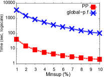
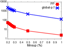
FIFA	Leviathan	Protein

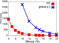
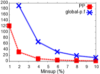
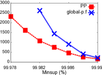
Figure 1: Comparing PP with global-p.f for SPM on real-life datasets: CPU times (top) and number of patterns (bottom).

5.2 Comparing with CP Methods for SPM

First we compare PP with the two CP encodings global-p.f and decomposed-p.f (see Section 3.2). Fig. 1 shows the number of extracted sequential patterns and the CPU times to extract them (in logscale for BIBLE, Kosarak and PubMed) for the three methods.

First, as expected, the lower $minsup$ is, the larger the number of extracted sequential patterns. Second, when comparing the CPU times, decomposed-p.f is the least performer method. On all the datasets, it fails to complete the extraction within the time limit for all values of $minsup$ we considered. Third, PP largely dominates global-p.f on all the datasets: PP is more than an order of magnitude faster than global-p.f. The gains in terms of CPU times are greatly amplified for low values of $minsup$. On BIBLE (resp. PubMed), the speed-up is $84.4$ (resp. $33.5$) for $minsup$ equal to $1\%$. Another important observation that can be made is that, on most of the datasets (except BIBLE and Kosarak), global-p.f is not able to mine for patterns at very low frequency within the time limit. For example on FIFA, PP is able to complete the extraction for values of $minsup$ up to $6\%$ in $1,457$ seconds, while global-p.f fails to complete the extraction for $minsup$ less than $10\%$. The same trend is also conformed on Leviathan, where global-p.f is not able to mine for patterns at $1\%$ minimum frequency.

To complement the results given by Fig. 1, Table 3 reports for different datasets and different values of $minsup$, the number of calls to the propagate routine of Gecode (column 5), and the number of nodes of the search tree (column 6). First, PP explores less nodes than global-p.f. But, the difference is not huge (gains of 45% and 33% on FIFA and BIBLE respectively). Second, our approach is very effective in terms of number of propagations. For PP, the number of propagations remains small (in thousands for small values of $minsup$) compared to global-p.f (in millions). This is due to the huge number of reified constraints used in global-p.f to encode the subsequence relation. On the contrary, our Prefix-Projection global constraint does not require any reified constraints nor any extra variables to encode the subsequence relation.

Dataset	$minsup$ (%)	#PATTERNS	CPU times (s)		#PROPAGATIONS		#NODES
			PP	global-p.f	PP	global-p.f	PP	global-p.f
FIFA	20	938	8.16	129.54	1884	11649290	1025	1873
	18	1743	13.39	222.68	3502	19736442	1922	3486
	16	3578	24.39	396.11	7181	35942314	3923	7151
	14	7313	44.08	704	14691	65522076	8042	14616
	12	16323	86.46	1271.84	32820	126187396	18108	32604
	10	40642	185.88	2761.47	81767	266635050	45452	81181
BIBLE	10	174	1.98	105.01	363	4189140	235	348
	8	274	2.47	153.61	575	5637671	362	548
	6	508	3.45	270.49	1065	8592858	669	1016
	4	1185	5.7	552.62	2482	15379396	1575	2371
	2	5311	15.05	1470.45	11104	39797508	7048	10605
	1	23340	41.4	3494.27	49057	98676120	31283	46557
PubMed	5	2312	8.26	253.16	4736	15521327	2833	4619
	4	3625	11.17	340.24	7413	20643992	4428	7242
	3	6336	16.51	536.96	12988	29940327	7757	12643
	2	13998	28.91	955.54	28680	50353208	17145	27910
	1	53818	77.01	2581.51	110133	124197857	65587	107051
Protein	99.99	127	165.31	219.69	264	26731250	172	221
	99.988	216	262.12	411.83	451	44575117	293	390
	99.986	384	467.96	909.47	805	80859312	514	679
	99.984	631	753.3	1443.92	1322	132238827	845	1119
	99.982	964	1078.73	2615	2014	201616651	1284	1749
	99.98	2143	2315.65	$-$	4485	$-$	2890	$-$
Kosarak	1	384	2.59	137.95	793	8741452	482	769
	0.5	1638	7.42	491.11	3350	26604840	2087	3271
	0.3	4943	19.25	1111.16	10103	56854431	6407	9836
	0.28	6015	22.83	1266.39	12308	64003092	7831	11954
	0.24	9534	36.54	1635.38	19552	81485031	12667	18966
	0.2	15010	57.6	2428.23	30893	111655799	20055	29713
Leviathan	10	651	1.78	12.56	1366	2142870	849	1301
	8	1133	2.57	19.44	2379	3169615	1487	2261
	6	2300	4.27	32.85	4824	5212113	3008	4575
	4	6286	9.08	66.31	13197	10569654	8227	12500
	2	33387	32.27	190.45	70016	33832141	43588	66116
	1	167189	121.89	$-$	350310	$-$	217904	$-$

Table 3: PP vs. global-p.f.

BIBLE	Kosarak	PubMed
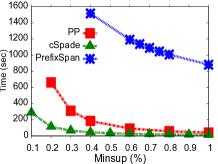
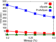
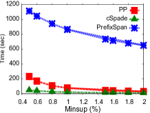
FIFA	Leviathan	Protein

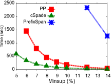
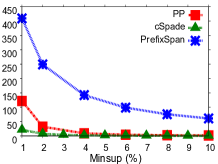
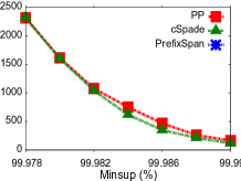
Figure 2: Comparing Prefix-Projection with state-of-the-art algorithms for SPM.

5.3 Comparing with ad hoc Methods for SPM

Our second experiment compares PP with state-of-the-art methods for SPM. Fig. 2 shows the CPU times of the three methods. First, cSpade obtains the best performance on all datasets (except on Protein). However, PP exhibits a similar behavior as cSpade, but it is less faster (not counting the highest values of $minsup$). The behavior of cSpade on Protein is due to the vertical representation format that is not appropriated in the case of databases having large sequences and small number of distinct items, thus degrading the performance of the mining process. Second, PP which also uses the concept of projected databases, clearly outperforms PrefixSpan on all datasets. This is due to our filtering algorithm combined together with incremental data structures to manage the projected databases. On FIFA, PrefixSpan is not able to complete the extraction for $minsup$ less than $12\%$, while our approach remains feasible until $6\%$ within the time limit. On Protein, PrefixSpan fails to complete the extraction for all values of $minsup$ we considered. These results clearly demonstrate that our approach competes well with state-of-the-art methods for SPM on large datasets and achieves scalability while it is a major issue of existing CP approaches.

5.4 SPM under size and item constraints

Our third experiment aims at assessing the interest of pushing simultaneously different types of constraints. We impose on the PubMed dataset usual constraints such as the minimum frequency and the minimum size constraints and other useful constraints expressing some linguistic knowledge such as the item constraint. The goal is to retain sequential patterns which convey linguistic regularities (e.g., gene - rare disease relationships) [3]. The size constraint allows to remove patterns that are too small w.r.t. the number of items (number of words) to be relevant patterns. We tested this constraint with $\ell_{min}$ set to 3. The item constraint imposes that the extracted patterns must contain the item GENE and the item DISEASE. As no ad hoc method exists for this combination of constraints, we only compare PP with global-p.f. Fig. 3 shows the CPU times and the number of sequential patterns extracted with and without constraints. First, pushing simultaneously the two constraints enables to reduce significantly the number of patterns. Moreover, the CPU times for PP decrease slightly whereas for global-p.f (with and without constraints), they are almost the same. This is probably due to the weak communication between the $m$ exists-embedding reified global constraints and the two constraints. This reduces significantly the quality of the whole filtering. Second (see Table 5), when considering the two constraints, PP clearly dominates global-p.f (speed-up value up to $51.5$). Moreover, the number of propagations performed by PP remains very small as compared to global-p.f. Fig. 3c compares the two methods under the minimum size constraint for different values of $\ell_{min}$, with $minsup$ fixed to $1\%$. Table 5 compares the two methods in terms of numbers of propagations (column $5$) and number of nodes of the search tree (column $6$). Once again, PP is always the most performer method (speed-up value up to $53.1$). These results also confirm what we observed previously, namely the weak communication between reified global constraints and constraints imposed on patterns (i.e., size and item constraints).

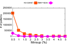
(a) # of patterns

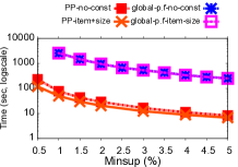
(b) CPU times (logscale)

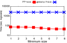
(c) Minimum size constraint

Figure 3: Comparing PP with global-p.f under minimum size and item constraints on PubMed.

Dataset	$minsup$ (%)	#PATTERNS	CPU times (s)		#PROPAGATIONS		#NODES
			PP	global-p.f	PP	global-p.f	PP	global-p.f
PubMed	5	279	6.76	252.36	7878	12234292	2285	4619
	4	445	8.81	339.09	12091	16475953	3618	7242
	3	799	12.35	535.32	20268	24380096	6271	12643
	2	1837	20.41	953.32	43088	42055022	13888	27910
	1	7187	49.98	2574.42	157899	107978568	52508	107051

Table 4: PP vs. global-p.f under minimum size and item constraints.

Dataset	$\ell_{min}$	#PATTERNS	CPU times (s)		#PROPAGATIONS		#NODES
			PP	global-p.f	PP	global-p.f	PP	global-p.f
PubMed	8	12	48.52	2577.09	55523	105343528	50264	107051
	6	3596	50.91	2576.9	59144	106272419	50486	107051
	4	40669	70.61	2579.3	96871	117781215	59194	107051
	2	53486	76.64	2580.41	109801	123913176	65334	107051
	1	53818	78.49	2579.85	110133	117208559	65587	107051

Table 5: PP vs. global-p.f under minimum size constraint.

5.5 SPM under regular constraints

Our last experiment compares PP-REG against two variants of SMA: SMA-1P (SMA one pass) and SMA-FC (SMA Full Check). Two datasets are considered from [18]: one synthetic dataset (data-200k), and one real-life dataset (Protein). For data-200k, we used two RE:

• $\mathtt{RE}10\equiv A^{*}B(B|C)D^{*}EF^{*}(G|H)I^{*}$,

• $\mathtt{RE}14\equiv A^{*}(Q|BS^{*}(B|C))D^{*}E(I|S)^{*}(F|H)G^{*}R$.

For Protein, we used $\mathtt{RE}2\equiv(S|T)$ . $(R|K)$ representing Protein kinase C phosphorylation (where . represents any symbol). Fig. 4 reports CPU-times comparison. On the synthetic dataset, our approach is very effective. For $\mathtt{RE}14$, our method is more than an order of magnitude faster than SMA. On Protein, the gap between the $3$ methods shrinks, but our method remains effective. For the particular case of $\mathtt{RE}2$, the Regular constraint can be substituted by restricting the domain of the first and third variables to $\{S,T\}$ and $\{R,K\}$ respectively (denoted as PP-SRE), thus improving performances.

data-200k (RE10)	data-200k (RE14)	Protein (RE2)

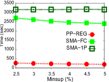
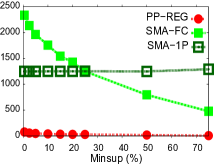
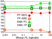
Figure 4: Comparing Prefix-Projection with SMA for SPM under RE constraint.

6 Conclusion

We have proposed the global constraint Prefix-Projection for sequential pattern mining. Prefix-Projection uses a concise encoding and provides an efficient filtering based on specific properties of the projected databases, and anti-monotonicity of the frequency constraint. When this global constraint is integrated into a CP solver, it enables to handle several constraints simultaneously. Some of them like size, item membership and regular expression are considered in this paper. Another point of strength, is that, contrary to existing CP approaches for SPM, our global constraint does not require any reified constraints nor any extra variables to encode the subsequence relation. Finally, although Prefix-Projection is well suited for constraints on sequences, it would require to be adapted to handle constraints on subsequence relations like gap.

Experiments performed on several real-life datasets show that our approach clearly outperforms existing CP approaches and competes well with ad hoc methods on large datasets and achieves scalability while it is a major issue of CP approaches. As future work, we intend to handle constraints on set of sequential patterns such as closedness, relevant subgroup and skypattern constraints.

References

- [1] Agrawal, R., Srikant, R.: Mining sequential patterns. In: Yu, P.S., Chen, A.L.P. (eds.) ICDE. pp. 3–14. IEEE Computer Society (1995)
- [2] Ayres, J., Flannick, J., Gehrke, J., Yiu, T.: Sequential pattern mining using a bitmap representation. In: KDD 2002. pp. 429–435. ACM (2002)
- [3] Béchet, N., Cellier, P., Charnois, T., Crémilleux, B.: Sequential pattern mining to discover relations between genes and rare diseases. In: CBMS (2012)
- [4] Beldiceanu, N., Contejean, E.: Introducing global constraints in CHIP. Journal of Mathematical and Computer Modelling 20(12), 97–123 (1994)
- [5] Coquery, E., Jabbour, S., Saïs, L., Salhi, Y.: A SAT-based approach for discovering frequent, closed and maximal patterns in a sequence. In: ECAI. pp. 258–263 (2012)
- [6] Fournier-Viger, P., Gomariz, A., Gueniche, T., Soltani, A., Wu, C., Tseng, V.: SPMF: A Java Open-Source Pattern Mining Library. J. of Machine Learning Resea. 15, 3389–3393 (2014)
- [7] Garofalakis, M.N., Rastogi, R., Shim, K.: Mining sequential patterns with regular expression constraints. IEEE Trans. Knowl. Data Eng. 14(3), 530–552 (2002)
- [8] Guns, T., Nijssen, S., Raedt, L.D.: Itemset mining: A constraint programming perspective. Artif. Intell. 175(12-13), 1951–1983 (2011)
- [9] Kemmar, A., Ugarte, W., Loudni, S., Charnois, T., Lebbah, Y., Boizumault, P., Crémilleux, B.: Mining relevant sequence patterns with cp-based framework. In: ICTAI. pp. 552–559 (2014)
- [10] Li, C., Yang, Q., Wang, J., Li, M.: Efficient mining of gap-constrained subsequences and its various applications. ACM Trans. Knowl. Discov. Data 6(1), 2:1–2:39 (Mar 2012)
- [11] Métivier, J.P., Loudni, S., Charnois, T.: A constraint programming approach for mining sequential patterns in a sequence database. In: ECML/PKDD Workshop on Languages for Data Mining and Machine Learning (2013)
- [12] Negrevergne, B., Guns, T.: Constraint-based sequence mining using constraint programming. In: CPAIOR’15 (also available as CoRR abs/1501.01178) (2015)
- [13] Novak, P.K., Lavrac, N., Webb, G.I.: Supervised descriptive rule discovery: A unifying survey of contrast set, emerging pattern and subgroup mining. Journal of Machine Learning Research 10 (2009)
- [14] Pei, J., Han, J., Mortazavi-Asl, B., Pinto, H., Chen, Q., Dayal, U., Hsu, M.: PrefixSpan: Mining sequential patterns by prefix-projected growth. In: ICDE. pp. 215–224. IEEE Computer Society (2001)
- [15] Pei, J., Han, J., Wang, W.: Mining sequential patterns with constraints in large databases. In: CIKM’02. pp. 18–25. ACM (2002)
- [16] Pesant, G.: A regular language membership constraint for finite sequences of variables. In: Wallace, M. (ed.) CP’04. LNCS, vol. 2239, pp. 482–495. Springer (2004)
- [17] Srikant, R., Agrawal, R.: Mining sequential patterns: Generalizations and performance improvements. In: EDBT. pp. 3–17 (1996)
- [18] Trasarti, R., Bonchi, F., Goethals, B.: Sequence mining automata: A new technique for mining frequent sequences under regular expressions. In: ICDM’08. pp. 1061–1066 (2008)
- [19] Yan, X., Han, J., Afshar, R.: CloSpan: Mining closed sequential patterns in large databases. In: Barbará, D., Kamath, C. (eds.) SDM. SIAM (2003)
- [20] Yang, G.: Computational aspects of mining maximal frequent patterns. Theor. Comput. Sci. 362(1-3), 63–85 (2006)
- [21] Zaki, M.J.: Sequence mining in categorical domains: Incorporating constraints. In: Proceedings of the 2000 ACM CIKM International Conference on Information and Knowledge Management, McLean, VA, USA, November 6-11, 2000. pp. 422–429 (2000)
- [22] Zaki, M.J.: SPADE: An efficient algorithm for mining frequent sequences. Machine Learning 42(1/2), 31–60 (2001)