Abstract

An original boundary integral formulation is proposed for the problem of a semi-infinite crack at the interface between two dissimilar elastic materials in the presence of heat flows and mass diffusion. Symmetric and skew-symmetric weight function matrices are used together with a generalized Betti’s reciprocity theorem in order to derive a system of integral equations that relate the applied loading, the temperature and mass concentration fields, the heat and mass fluxes on the fracture surfaces and the resulting crack opening. The obtained integral identities can have many relevant applications, such as for the modelling of crack and damage processes at the interface between different components in electrochemical energy devices characterized by multi-layered structures (solid oxide fuel cells and lithium ions batteries).

Keywords: Interfacial crack, Thermodiffusion, Betty reciprocity theorem, Lamé potentials, Singular integral equations.

1 Introduction

Modelling of interfacial crack problems in elastic bimaterials in presence of thermodiffusion represents an important issue for many engineering applications. In particular, it is crucial for studying fracture initiation and propagation at the interface between different components of electrochemical energy devices which are characterized by multi-layered structures, such as solid oxide fuel cells and lithium ions batteries. Indeed, due to the high operational temperature that can be reached and to the intense particle fluxes that are required for maintaining the electrical current, the components of these devices are subject to severe thermomechanical stresses as well as stresses induced by the particle diffusion (Anandakumar et al., 2010; Zhang et al., 2010). This can cause damage and crack formation compromising their performances in terms of power generation and energy conversion efficiency (Lowrie and Rawlings, 2000; Malzbender et al., 2003; Goutianos et al., 2010; Zhao et al., 2010; Pharr et al., 2013). For this reason, the modelling of fracture processes at the interface between the components of such battery devices is fundamental to the prediction of these phenomena, and subsequently enables successful manufacture and reliable performances of the systems.

Due to their distinctive feature of reducing by one the dimension of the considered problems, so that only the boundary or surface of the domain needs to be modeled, boundary integral formulations are particularly suitable for studying multiphysics phenomena such as dynamic and static fracture processes in thermodiffusive elastic materials. Several boundary integral approaches have been proposed for solving crack problems in linear elastic, thermoelastic and thermodiffusive materials, such as analytical techniques based on the method of singular integral equations (Weaver, 1977; Budiansky and Rice, 1979; Linkov et al., 1997), and numerical techniques based on the boundary element method (Rizzo and Shippy, 1977; Brebbia et al., 1984; Sladek and Sladek, 1983, 1984a, 1984b). In all these approaches, the displacements and stress fields are defined by integral relations involving the Green’s functions, which need to be derived analytically in explicit form (Bigoni and Capuani, 2002) or computed numerically (Ang and Telles, 2004). Altough Green’s functions have been derived for several crack problems in linear thermoelastic and thermodiffusive elastic materials (Sturla and Barber, 1988; Hou et al., 2008; Kumar and Chawla, 2012a, b), their utilization for calculating physical displacements and stress fields on the crack faces requires challenging numerical estimation of integrals whose convergence should be assessed carefully. Moreover, the approach based on the Green’s function method works when the tractions and the thermal and diffusive stresses acting on the discontinuity surface are symmetric, but not in the case where asymmetric mechanical and thermodiffusive loading distributions are applied on the crack faces.

In this paper, the problem of a semi-infinite quasi-static crack at the interface between two dissimilar thermodiffusive elastic materials is addressed by means of an origianl boundary integral formulation which avoids the use of the Green’s functions and the challenging computations connected, without any assumptions regarding the symmetry of the loading and of the temperature and mass concentration profile at the interface. The general approach recently proposed in Piccolroaz and Mishuris (2013); Morini et al. (2013a); Vellender et al. (2013) and Mishuris et al. (2014) for interfacial crack problems in isotropic and anisotropic elastic bimaterials, based on Betti’s reciprocal theorem and weight functions theory, is extended in order to study fracture processes in presence of thermodiffusion. The volume integral terms present in the reciprocity identity, associated with the temperature and mass concentration effects (Nowacki, 1974a), are converted into surface integrals through an exact transformation based on the notion of Lamé elastic potentials (Slaughter, 2001) while assuming that the temperature and mass concentration are harmonic in the domain. The derived original form of Betti’s identity is used together with symmetric and skew-symmetric weight function matrices derived by Piccolroaz and Mishuris (2013) for formulating the considered crack problem in thermodiffusive bimaterials in terms of singular integral equations.

The article is organized as follows: in Section 2, the static governing equations for a linear elastic thermodiffusive media are formulated. Reciprocity indetities are introduced and the volume integral terms associated with the temperature and mass concentration fields are transformed into boundary surface integrals by introducing Lamé elastic potentials and applying second Green’s theorem. In Section 3, the problem of a quasi-static crack at the interface bewteen two dissimilar elastic thermodiffusive media is introduced. The weight functions, defined as a special singular solution of the homogeneous traction-free problem are used together with the obtained Betti’s identity for formulating the problem in terms of boundary integral equations. The case of a plane strain crack is analysed in Section 4. Lamé potentials in the weight functions space are derived in closed form, and explicit integral identities relating the applied mechanical loading, the profiles of temperature, mass concentration, heat and mass fluxes on the interface and the resulting crack opening are obtained. Finally, in Section 5, the integral identities are used to study some illustrative examples of plane crack problems in the presence of thermodiffusion. Exact expressions for the crack opening and tractions ahead of the crack tip associated with the introduced temperature and heat flux distributions are derived, and the corresponding stress intensity factors are calculated in closed form.

2 Preliminary results: governing equations and reciprocity theorem

In this Section, constitutive relations and static balance equation for linear thermodiffusive elastic media in infinitesimal deformations are introduced. Betti’s integral identities are derived by means of the theorem of the reciprocity of work, and volume integral terms associated with heat flows and mass diffusion are converted into surface integrals using an exact transformation based on the introduction of Lamé elastic potentials.

2.1 Governing equations

For a linear isotropic elastic body where temperature changes and mass diffusion are considered, the constitutive relationship between the stress ${\sigma}$ and the strain ${\varepsilon}$ is given by (Nowacki, 1974a):

$$\mbox{\boldmath${\sigma}$}=2\mu\mbox{\boldmath${\varepsilon}$}+\left(\lambda\mbox{tr}\mbox{\boldmath${\varepsilon}$}-\gamma_{t}\theta-\gamma_{c}\chi\right)\mbox{\boldmath$I$},$$ (1)

where $\lambda$ and $\mu$ are Lamé’s constants, $\theta=T-T_{0}$ is the temperature of the medium with respect to the reference state ($\mbox{\boldmath${\varepsilon}$}=0,\ T=T_{0}\ C=C_{0})$, $\chi=C-C_{0}$ is the concentration of diffusing particles with respect to the natural state, $I$ is the identity matrix, $\gamma_{t}=(3\lambda+2\mu)\alpha_{t}$ and $\gamma_{c}=(3\lambda+2\mu)\alpha_{c}$ with $\alpha_{t}$ and $\alpha_{c}$ coefficients of thermal and diffusive expansions, respectively. Then in the natural state of the system we have

$$\mbox{\boldmath${\varepsilon}$}=0,\quad\theta=0,\quad\chi=0,$$ (2)

and in order to describe the material using linear thermoelastic diffusion theory (Nowacki, 1974a; Sherief et al., 2004) the values of $\theta$ and $\chi$ are assumed such that $|\theta/T_{0}|\ll 1$ and $|\chi/C_{0}|\ll 1$.

In the static case, the equations of equilibrium are given by

$$\nabla\cdot\mbox{\boldmath${\sigma}$}+\mbox{\boldmath$b$}=0,$$ (3)

where $b$ represents the body forces. Substituting the constitutive relation (1) in (3), the Navier’s equations in terms of displacements $u$ are obtained

$$\mu\Delta\mbox{\boldmath$u$}+(\lambda+\mu)\nabla(\nabla\cdot\mbox{\boldmath$u$})+\mbox{\boldmath$b$}=\gamma_{t}\nabla\theta+\gamma_{c}\nabla\chi.$$ (4)

The conservation of energy and mass in steady-state conditions leads to

$$\nabla\cdot\mbox{\boldmath$q$}=W,\quad\nabla\cdot\mbox{\boldmath$j$}=0,$$ (5)

where $W$ is the heat generated for unit of time and volume by internal sources. For the considered linear isotropic thermodiffusive media, the heat flux $q$ and particles current $j$ can be expressed as

$$\mbox{\boldmath$q$}=-k_{t}\nabla\theta,\quad\mbox{\boldmath$j$}=-D_{c}\nabla\chi,$$ (6)

where $k_{t}$ is the thermal conductivity coefficient and $D_{c}$ is the mass diffusivity of the material. Using relations (6) in (5), the following Poisson’s and Laplace’s equations for the steady-state temperature and mass concentration fields are derived:

$$k_{t}\Delta\theta+W=0,\quad\Delta\chi=0.$$ (7)

2.2 Reciprocity theorem: transformation of the volume integrals

Let us consider a thermodiffusive elastic body of volume $V$ subject to the action of body forces $\mbox{\boldmath$b$}^{(1)}$, tractions $\mbox{\boldmath$t$}^{(1)}$, heat sources $W^{(1)}$, surface heating to the temperature $\theta_{b}^{(1)}$ and mass concentration on the boundary $\chi_{b}^{(1)}$. These causes are written symbolically in the compact form

$$\mathcal{I}^{(1)}=\left\{\mbox{\boldmath$b$}^{(1)},\mbox{\boldmath$t$}^{(1)},W^{(1)},\theta_{b}^{(1)},\chi_{b}^{(1)}\right\},$$ (8)

and produce in the body the state characterized by displacements $\mbox{\boldmath$u$}^{(1)}(\mbox{\boldmath$x$})$, temperature $\theta^{(1)}(\mbox{\boldmath$x$})$ and mass concentration $\chi^{(1)}(\mbox{\boldmath$x$})$:

$$\mathcal{C}^{(1)}=\left\{\mbox{\boldmath$u$}^{(1)}(\mbox{\boldmath$x$}),\ \theta^{(1)}(\mbox{\boldmath$x$}),\ \chi^{(1)}(\mbox{\boldmath$x$})\right\},\quad\mbox{\boldmath$x$}\in V.$$ (9)

The stresses $\mbox{\boldmath${\sigma}$}^{(1)}$ and the strains $\mbox{\boldmath${\varepsilon}$}^{(1)}$ are connected by the relationship (1), where the dilatation is defined as $\mbox{tr}\mbox{\boldmath${\varepsilon}$}=\nabla\cdot\mbox{\boldmath$u$}$, and they are assumed to be continuous together with their first derivatives. The displacements, temperature and mass concentration are also continuous and moreover have continuous derivatives up to the second order for $\mbox{\boldmath$x$}\in V+\partial V$. These functions satisfy the fields equations (3), (7)₍₁₎ and (7)₍₂₎ with boundary conditions:

$$\mbox{\boldmath$t$}^{(1)}(\mbox{\boldmath$x$})=\mbox{\boldmath${\sigma}$}^{(1)}(\mbox{\boldmath$x$})\mbox{\boldmath$n$}(\mbox{\boldmath$x$}),\quad\mbox{\boldmath$x$}\in\partial V,$$ (10)

and

$$\theta^{(1)}(\mbox{\boldmath$x$})=\theta_{b}^{(1)}(\mbox{\boldmath$x$}),\quad\chi^{(1)}(\mbox{\boldmath$x$})=\chi_{b}^{(1)}(\mbox{\boldmath$x$}),\quad\mbox{\boldmath$x$}\in\partial V,$$ (11)

where $n$ denotes the unit outward normal to the surface $\partial V$.

Introducing another set of causes $\mathcal{I}^{(2)}$ and effects $\mathcal{C}^{(2)}$:

$$\mathcal{I}^{(2)}=\left\{\mbox{\boldmath$b$}^{(2)},Q^{(2)},\mbox{\boldmath$t$}^{(2)},\theta_{b}^{(2)},\chi_{b}^{(2)}\right\},\quad\mathcal{C}^{(2)}=\left\{\mbox{\boldmath$u$}^{(2)}(\mbox{\boldmath$x$}),\ \theta^{(2)}(\mbox{\boldmath$x$}),\ \chi^{(2)}(\mbox{\boldmath$x$})\right\},$$ (12)

and applying the procedure illustrated in Nowacki (1974a, b) for elastic thermodiffusive media, the following reciprocity integral relations bewteen the two systems of causes and results are derived:

$$\int_{\partial V}\left(\mbox{\boldmath${\sigma}$}^{(1)}\mbox{\boldmath$n$}\cdot\mbox{\boldmath$u$}^{(2)}-\mbox{\boldmath${\sigma}$}^{(2)}\mbox{\boldmath$n$}\cdot\mbox{\boldmath$u$}^{(1)}\right)dS+\int_{V}\left(\mbox{\boldmath$b$}^{(1)}\cdot\mbox{\boldmath$u$}^{(2)}-\mbox{\boldmath$b$}^{(2)}\cdot\mbox{\boldmath$u$}^{(1)}\right)dV+$$

$$+\gamma_{t}\int_{V}\left(\theta^{(1)}\nabla\cdot\mbox{\boldmath$u$}^{(2)}-\theta^{(2)}\nabla\cdot\mbox{\boldmath$u$}^{(1)}\right)dV+\gamma_{c}\int_{V}\left(\chi^{(1)}\nabla\cdot\mbox{\boldmath$u$}^{(2)}-\chi^{(2)}\nabla\cdot\mbox{\boldmath$u$}^{(1)}\right)dV=0,$$ (13)

$$k_{t}\int_{\partial V}\left(\nabla\theta^{(1)}\theta^{(2)}-\nabla\theta^{(2)}\theta^{(1)}\right)\cdot\mbox{\boldmath$n$}\ dS+\int_{V}\left(W^{(1)}\theta^{(2)}-W^{(2)}\theta^{(1)}\right)dV=0,$$ (14)

$$\int_{\partial V}\left(\nabla\chi^{(1)}\chi^{(2)}-\nabla\chi^{(2)}\chi^{(1)}\right)\cdot\mbox{\boldmath$n$}\ dS=0.$$ (15)

Expressions (13) and (14) have been extensively used in the literature in order to develop numerical buondary elements methods for studying both static and dynamic crack problems in elastic materials subject to thermal stresses (Sladek and Sladek, 1983, 1984a, 1984b; Dell’Erba et al., 1998). In most of these approaches, starting from equations (13) and (14), integral expressions for the physical displacements, stresses and temperature $\mbox{\boldmath$u$}^{(1)},\mbox{\boldmath${\sigma}$}^{(1)}$ and $\theta^{(1)}$, are derived as functions of the test quantities $\mbox{\boldmath$u$}^{(2)},\mbox{\boldmath${\sigma}$}^{(2)}$ and $\theta^{(2)}$, which in general are assumed to be fundamental solutions of the evolution equations or weight functions (Brebbia et al., 1984; Rizzo and Shippy, 1977). Several analytical and numerical transformations have been proposed for reducing the volume integrals associated with body forces and coupling between mechanical strains and temperature to surface integrals (Shiah and Tan, 1999, 2012).

Here, we assume zero body forces and heat sources acting on the system, and we introduce an exact procedure for transforming coupling volume terms involving temperature and mass concentration in equation (13). From Helmholtz’s decomposition theorem, since both the displacements $\mbox{\boldmath$u$}^{(1)}$, $\mbox{\boldmath$u$}^{(2)}$ are solutions of the equilibrium equation (4), they can be represented by scalar displacement potentials $\varphi^{(1)},\varphi^{(2)}$ and vector displacement potentials $\mbox{\boldmath${\psi}$}^{(1)},\mbox{\boldmath${\psi}$}^{(2)}$ (Slaughter, 2001):

$$\mbox{\boldmath$u$}^{(1)}=\nabla\varphi^{(1)}+\nabla\times\mbox{\boldmath${\psi}$}^{(1)},\quad\mbox{\boldmath$u$}^{(2)}=\nabla\varphi^{(2)}+\nabla\times\mbox{\boldmath${\psi}$}^{(2)},$$ (16)

substituting expressions (16) into (13), the following equation is obtained:

$$\int_{\partial V}\left(\mbox{\boldmath${\sigma}$}^{(1)}\mbox{\boldmath$n$}\cdot\mbox{\boldmath$u$}^{(2)}-\mbox{\boldmath${\sigma}$}^{(2)}\mbox{\boldmath$n$}\cdot\mbox{\boldmath$u$}^{(1)}\right)dS+$$

$$+\gamma_{t}\int_{V}\left(\theta^{(1)}\Delta\varphi^{(2)}-\theta^{(2)}\Delta\varphi^{(1)}\right)dV+\gamma_{c}\int_{V}\left(\chi^{(1)}\Delta\varphi^{(2)}-\chi^{(2)}\Delta\varphi^{(1)}\right)dV=0.$$ (17)

The Green’s second identity states that two arbitrary scalar functions, $\phi$ and $\vartheta$, must satisfy

$$\int_{V}\left(\phi\Delta\vartheta-\vartheta\Delta\phi\right)dV=\int_{\partial V}\left(\phi\nabla\vartheta-\vartheta\nabla\phi\right)\cdot\mbox{\boldmath$n$}\ dS.$$ (18)

Substituting respectively $\theta^{(1)},\theta^{(2)},\chi^{(1)},\chi^{(2)}$ to $\vartheta$ and $\varphi^{(1)},\varphi^{(2)}$ to $\phi$, using equations (7) and remembering that zero heating sources are assumed, we get

$$\int_{V}\theta^{(1)}\Delta\varphi^{(2)}dV=\int_{\partial V}\left(\theta^{(1)}\nabla\varphi^{(2)}-\varphi^{(2)}\nabla\theta^{(1)}\right)\cdot\mbox{\boldmath$n$}\ dS,$$ (19)

$$\int_{V}\theta^{(2)}\Delta\varphi^{(1)}dV=\int_{\partial V}\left(\theta^{(2)}\nabla\varphi^{(1)}-\varphi^{(1)}\nabla\theta^{(2)}\right)\cdot\mbox{\boldmath$n$}\ dS,$$ (20)

$$\int_{V}\chi^{(1)}\Delta\varphi^{(2)}dV=\int_{\partial V}\left(\chi^{(1)}\nabla\varphi^{(2)}-\varphi^{(2)}\nabla\chi^{(1)}\right)\cdot\mbox{\boldmath$n$}\ dS,$$ (21)

$$\int_{V}\chi^{(2)}\Delta\varphi^{(1)}dV=\int_{\partial V}\left(\chi^{(2)}\nabla\varphi^{(1)}-\varphi^{(1)}\nabla\chi^{(2)}\right)\cdot\mbox{\boldmath$n$}\ dS,$$ (22)

substituting expressions (19)-(22) into (17), we finally derive

$$\int_{\partial V}\left(\mbox{\boldmath${\sigma}$}^{(1)}\mbox{\boldmath$n$}\cdot\mbox{\boldmath$u$}^{(2)}-\mbox{\boldmath${\sigma}$}^{(2)}\mbox{\boldmath$n$}\cdot\mbox{\boldmath$u$}^{(1)}\right)dS+$$

$$+\gamma_{t}\int_{\partial V}\left(\theta^{(1)}\nabla\varphi^{(2)}-\varphi^{(2)}\nabla\theta^{(1)}-\theta^{(2)}\nabla\varphi^{(1)}+\varphi^{(1)}\nabla\theta^{(2)}\right)\cdot\mbox{\boldmath$n$}\ dS+$$

$$+\gamma_{c}\int_{\partial V}\left(\chi^{(1)}\nabla\varphi^{(2)}-\varphi^{(2)}\nabla\chi^{(1)}-\chi^{(2)}\nabla\varphi^{(1)}+\varphi^{(1)}\nabla\chi^{(2)}\right)\cdot\mbox{\boldmath$n$}\ dS=0.$$ (23)

By means of the proposed general procedure, the volume integral terms associated with thermal and diffusive stresses in the reciprocity identity (17) has been reduced to surface integrals. Remembering the fluxes definitions (6), expression (23) can be written as follows

$$\int_{\partial V}\left(\mbox{\boldmath${\sigma}$}^{(1)}\mbox{\boldmath$n$}\cdot\mbox{\boldmath$u$}^{(2)}-\mbox{\boldmath${\sigma}$}^{(2)}\mbox{\boldmath$n$}\cdot\mbox{\boldmath$u$}^{(1)}\right)dS+$$

$$+\gamma_{t}\int_{\partial V}\left(\theta^{(1)}\nabla\varphi^{(2)}-\theta^{(2)}\nabla\varphi^{(1)}\right)\cdot\mbox{\boldmath$n$}\ dS+\beta_{t}\int_{\partial V}\left(\varphi^{(2)}\mbox{\boldmath$q$}^{(1)}-\varphi^{(1)}\mbox{\boldmath$q$}^{(2)}\right)\cdot\mbox{\boldmath$n$}\ dS+$$

$$+\gamma_{c}\int_{\partial V}\left(\chi^{(1)}\nabla\varphi^{(2)}-\chi^{(2)}\nabla\varphi^{(1)}\right)\cdot\mbox{\boldmath$n$}\ dS+\beta_{c}\int_{\partial V}\left(\varphi^{(2)}\mbox{\boldmath$j$}^{(1)}-\varphi^{(1)}\mbox{\boldmath$j$}^{(2)}\right)\cdot\mbox{\boldmath$n$}\ dS=0,$$ (24)

where $\beta_{t}=\gamma_{t}/k_{t}$ and $\beta_{c}=\gamma_{t}/D_{c}$. Assuming $W=0$, reciprocity identities (14) and (15) can also be expressed in terms of fluxes:

$$\int_{\partial V}\left(\mbox{\boldmath$q$}^{(2)}\theta^{(1)}-\mbox{\boldmath$q$}^{(1)}\theta^{(1)}\right)\cdot\mbox{\boldmath$n$}\ dS=0,\quad\int_{\partial V}\left(\mbox{\boldmath$j$}^{(2)}\chi^{(1)}-\mbox{\boldmath$j$}^{(1)}\chi^{(2)}\right)\cdot\mbox{\boldmath$n$}\ dS=0.$$ (25)

In the cases where it is possible to determine explicitly the elastic potentials (16), using expression (24) together with (25) boundary integral formulation of static crack problems in thermodiffusive solids can be obtained avoiding numerical estimation of volume integrals (Cheng et al., 2001). In the next Sections, the obtained relation (24) will be extensively applied in order to derive integral identities for the modelling of fracture phenomena at the interface between dissimilar elastic materials in presence of thermodiffusion.

Figure 1: Geometry of the model.

3 Interfacial cracks in thermodiffusive media

A static semi-infinite crack between two dissimilar elastic materials in presence of thermodiffusion is condidered, the geometry of the system is shown in Fig.1. No body forces, heat and mass sources are assumed. The crack is situated in the half-plane $\mathbb{R}^{2}_{-}=\left\{\mbox{\boldmath$x$}=(x_{1},x_{2},x_{3})\in\mathbb{R}^{3}:x_{1}<0,x_{2}=0\right\}$, and general non-symmetric loading applied to the crack faces is assumed. Further in the text, we will use the superscripts ⁺ and ^- to denote the quantities related to the upper and the lower elastic thermodiffusive half-spaces, respectively. The applied loading can be decomposed in the symmetrical and skew-symmetrical parts, which are defined as follows (Piccolroaz et al., 2009):

$$\left\langle\mbox{\boldmath$p$}\right\rangle=\frac{1}{2}\left(\mbox{\boldmath$p$}^{+}+\mbox{\boldmath$p$}^{-}\right),\quad[\mbox{}[\mbox{\boldmath$p$}]\mbox{}]=\mbox{\boldmath$p$}^{+}-\mbox{\boldmath$p$}^{-},$$ (26)

where we used standard notations to denote the average, $\langle f\rangle$, and the jump, $[\mbox{}[f]\mbox{}]$, of a function $f$ across the plane containing the crack, $x_{2}=0$,

$$\left\langle f\right\rangle(x_{1},x_{3})=\frac{1}{2}[f(x_{1},0^{+},x_{3})+f(x_{1},0^{-},x_{3})],\quad[\mbox{}[f]\mbox{}](x_{1},x_{3})=f(x_{1},0^{+},x_{3})-f(x_{1},0^{-},x_{3}).$$ (27)

In the proposed model, thermal conduction and diffusion are both assumed to be isotropic, and then only normal stresses are induced by temperature changes and mass diffusion (see constitutive relation (1)).

Further in the paper, using the Betti identities (24) and (25), the considered crack problem will be formulated in terms of boundary integral equations. In order to correctly apply expressions (24) and (25), a preliminary discussion regarding the behaviour of the temperature and mass concentration functions in the upper and lower elastic thermodiffusive half-spaces is reported in next Section 3.1, and boundary conditions for these fields and the fluxes (6) are introduced.

3.1 Temperature and mass concentration in thermodiffusive half-spaces

Since zero heat and mass sources are assumed, the temperature $\theta$ and mass concentration fields are harmonic functions determined by the solution of a Laplace’s equation assuming the form of (7)₍₂₎. Considering the upper elastic thermodiffusive half-space these equations become

$$\Delta\theta^{+}=0,\quad\Delta\chi^{+}=0,\quad x_{2}>0.$$ (28)

Note that the conditions of harmonicity of the temperature and concentration fields (28) must be satisfied in order to transform the volume integrals involved in the reciprocity identity (17) in surface integrals following the procedure explained in Section 2.2.

The values of $\theta$ and $\chi$ for $x_{2}=0^{+}$, corresponding to the plane containing both the bounded interface and the crack, are given by:

$$\theta^{+}(x_{2}=0^{+})=\theta(x_{1},0^{+},x_{3}),\quad\chi^{+}(x_{2}=0^{+})=\chi(x_{1},0^{+},x_{3}).$$ (29)

Replacing $\theta^{+}$ with $\theta^{-}$ and $\chi^{+}$ with $\chi^{-}$ a couple of Laplace’s equations identical to the (28) and defined for $x_{2}<0$ are obtained for the lower thermodiffusive half-space, and then for $x_{2}=0^{-}$ boundary conditions analgous to (29) can be written.

The average and the jump of the temperature and concentration are defined on the whole plane $x_{2}=0$:

$$\left\langle\theta\right\rangle(x_{1},x_{3})=\frac{1}{2}[\theta(x_{1},0^{+},x_{3})+\theta(x_{1},0^{-},x_{3})],\quad-\infty<x_{1},x_{3}<+\infty,$$

$$\left\langle\chi\right\rangle(x_{1},x_{3})=\frac{1}{2}[\chi(x_{1},0^{+},x_{3})+\chi(x_{1},0^{-},x_{3})],\quad-\infty<x_{1},x_{3}<+\infty,$$ (30)

$$[\mbox{}[\theta]\mbox{}](x_{1},x_{3})=\theta(x_{1},0^{+},x_{3})-\theta(x_{1},0^{-},x_{3}),\quad-\infty<x_{1},x_{3}<+\infty,$$

$$[\mbox{}[\chi]\mbox{}](x_{1},x_{3})=\chi(x_{1},0^{+},x_{3})-\chi(x_{1},0^{-},x_{3}),\quad-\infty<x_{1},x_{3}<+\infty.$$ (31)

Further in the text, we will refer to (30) and (31) as to imperfect thermodiffusive interface conditions. The values of the components of the fluxes normal to the interface plane, $q_{2}=\mbox{\boldmath$q$}\cdot\mbox{\boldmath$e$}_{2}$ and $j_{2}=\mbox{\boldmath$j$}\cdot\mbox{\boldmath$e$}_{2}$, for $x_{2}=0^{+}$ are

$$q_{2}^{+}(x_{2}=0^{+})=-\left.k_{t}^{+}\frac{\partial\theta^{+}}{\partial x_{2}}\right|_{x_{2}=0^{+}}=q_{2}(x_{1},0^{+},x_{3}),\quad j_{2}^{+}(x_{2}=0^{+})=-\left.D_{c}^{+}\frac{\partial\chi^{+}}{\partial x_{2}}\right|_{x_{2}=0^{+}}=j_{2}(x_{1},0^{+},x_{3}),\$$ (32)

and similarly to the cases of temperature and mass concentration, expressions analogous to the (32) can be defined for the normal fluxes in the limit $x_{2}=0^{-}$.

The average and the jump of of $q_{2}$ and $j_{2}$ are also defined on the whole plane $x_{2}=0$:

$$\left\langle q_{2}\right\rangle(x_{1},x_{3})=\frac{1}{2}[q_{2}(x_{1},0^{+},x_{3})+q_{2}(x_{1},0^{-},x_{3})],\quad-\infty<x_{1},x_{3}<+\infty,$$

$$\left\langle j_{2}\right\rangle(x_{1},x_{3})=\frac{1}{2}[j_{2}(x_{1},0^{+},x_{3})+j_{2}(x_{1},0^{-},x_{3})],\quad-\infty<x_{1},x_{3}<+\infty,$$ (33)

$$[\mbox{}[q_{2}]\mbox{}](x_{1},x_{3})=q_{2}(x_{1},0^{+},x_{3})-q_{2}(x_{1},0^{-},x_{3}),\quad-\infty<x_{1},x_{3}<+\infty,$$

$$[\mbox{}[j_{2}]\mbox{}](x_{1},x_{3})=j_{2}(x_{1},0^{+},x_{3})-j_{2}(x_{1},0^{-},x_{3}),\quad-\infty<x_{1},x_{3}<+\infty.$$ (34)

Both in the upper and lower half spaces, the temperatures and mass concentration fields are assumed to vanish at the infinity:

$$\theta^{+}=\chi^{+}=0,\ \mbox{for}\ x_{1},x_{3}\rightarrow\pm\infty,\quad\theta^{+}=\chi^{+}=0,\mbox{for}\ x_{2}\rightarrow+\infty,$$

$$\theta^{-}=\chi^{-}=0,\ \mbox{for}\ x_{1},x_{3}\rightarrow\pm\infty,\quad\theta^{-}=\chi^{-}=0,\mbox{for}\ x_{2}\rightarrow-\infty.$$ (35)

Since the heat and mass conduction problems (28) are stationary, the flux functions $q_{2}$ and $j_{2}$ must satisfy the self-balance conditions on the boundary. For the considered upper thermodiffusive half-plane this means that:

$$\iint_{-\infty}^{+\infty}q_{2}(x_{1},0^{+},x_{3})dx_{1}dx_{3}=0,\quad\iint_{-\infty}^{+\infty}j_{2}(x_{1},0^{+},x_{3})dx_{1}dx_{3}=0,$$ (36)

where the definitions (32) for the values of the fluxes on the interface plane $x=0$ have been utilized. Note that the self-balance conditions for the fluxes on $x_{2}=0^{-}$ are given by relations similar to the (36). Remembering the definitions (33) and (34), integral balance conditions analogues to the (36) can be derived for the average and jump of the fluxes across the plane $x_{2}=0$.

3.2 Boundary integral equations

Considering the geometry of the model shown in Fig. 1, the Betti identities (24) and (25) are applied to a semi-spherical domain of radius $r$ in the upper and in the lower half spaces $\mathbb{R}^{3}_{+}$ and $\mathbb{R}^{3}_{-}$. In the limit $r\rightarrow\infty$, assuming that both the displacement fields $\mbox{\boldmath$u$}^{(1)}$ and $\mbox{\boldmath$u$}^{(2)}$ decay suitably fast at infinity and remembering conditions (35) for the temperature and mass concentration fields, the reciprocity relation (24) in the upper half-space becomes:

$$\int_{(x_{2}=0^{+})}\left[\mbox{\boldmath${\sigma}$}_{2}^{(1)}(x_{1},0^{+},x_{3})\cdot\mbox{\boldmath$u$}^{(2)}(x_{1},0^{+},x_{3})-\mbox{\boldmath${\sigma}$}_{2}^{(2)}(x_{1},0^{+},x_{3})\cdot\mbox{\boldmath$u$}^{(1)}(x_{1},0^{+},x_{3})\right]\ dx_{1}dx_{3}+$$

$$+\gamma_{t}^{+}\int_{(x_{2}=0^{+})}\left[\theta^{(1)}(x_{1},0^{+},x_{3})\frac{\partial\varphi^{(2)}(x_{1},0^{+},x_{3})}{\partial x_{2}}-\theta^{(2)}(x_{1},0^{+},x_{3})\frac{\partial\varphi^{(1)}(x_{1},0^{+},x_{3})}{\partial x_{2}}\right]\ dx_{1}dx_{3}+$$

$$+\beta_{t}^{+}\int_{(x_{2}=0^{+})}\left[\varphi^{(2)}(x_{1},0^{+},x_{3})q_{2}^{(1)}(x_{1},0^{+},x_{3})-\varphi^{(1)}(x_{1},0^{+},x_{3})q_{2}^{(2)}(x_{1},0^{+},x_{3})\right]\ dx_{1}dx_{3}+$$

$$+\gamma_{c}^{+}\int_{(x_{2}=0^{+})}\left[\chi^{(1)}(x_{1},0^{+},x_{3})\frac{\partial\varphi^{(2)}(x_{1},0^{+},x_{3})}{\partial x_{2}}-\chi^{(2)}(x_{1},0^{+},x_{3})\frac{\partial\varphi^{(1)}(x_{1},0^{+},x_{3})}{\partial x_{2}}\right]\ dx_{1}dx_{3}+$$

$$+\beta_{c}^{+}\int_{(x_{2}=0^{+})}\left[\varphi^{(2)}(x_{1},0^{+},x_{3})j_{2}^{(1)}(x_{1},0^{+},x_{3})-\varphi^{(1)}(x_{1},0^{+},x_{3})j_{2}^{(2)}(x_{1},0^{+},x_{3})\right]\ dx_{1}dx_{3}=0,$$ (37)

where $\mbox{\boldmath$u$}=[u_{1},u_{2},u_{3}]^{T}$ and $\mbox{\boldmath${\sigma}$}_{2}$ denotes the traction vector acting on the plane $x_{2}=0$: $\mbox{\boldmath${\sigma}$}_{2}=\mbox{\boldmath${\sigma}$}\mbox{\boldmath$e$}_{2}$. In the same limit $r\rightarrow\infty$, expressions (25) assume the following form:

$$\int_{(x_{2}=0^{+})}\left[\theta^{(1)}(x_{1},0^{+},x_{3})q_{2}^{(1)}(x_{1},0^{+},x_{3})-\theta^{(2)}(x_{1},0^{+},x_{3})q_{2}^{(2)}(x_{1},0^{+},x_{3})\right]\ dx_{1}dx_{3}=0,$$ (38)

$$\int_{(x_{2}=0^{+})}\left[\chi^{(1)}(x_{1},0^{+},x_{3})j^{(2)}_{2}(x_{1},0^{+},x_{3})-\chi^{(2)}(x_{1},0^{+},x_{3})j^{(1)}_{2}(x_{1},0^{+},x_{3})\right]\ dx_{1}dx_{3}=0.$$ (39)

Considering the boundary $x=0^{-}$ instead of $x=0^{+}$, three similar expressions are derived for the lower half-space. In the cases where elastic potentials can be derived explicitly, integral equations (37), (38) and (39) can be used together with their analogues in the lower half-plane in order to obtain expressions for the physical fields associated with the crack problem $\mbox{\boldmath$u$}^{(1)},\mbox{\boldmath${\sigma}$}_{2}^{(1)},\theta^{(1)},q_{2}^{(1)},\chi^{(1)}$ and $j_{2}^{(1)}$. These physical quantities are evaluated by means of a set of predetermined auxiliary functions $\mbox{\boldmath$u$}^{(2)},\mbox{\boldmath${\sigma}$}_{2}^{(2)},\theta^{(2)},q_{2}^{(2)},\chi^{(2)}$ and $j_{2}^{(2)}$ satisfying the balance equations.

3.3 Betti formula and weight functions

Following the approach proposed in several boundary element formulations of thermoelasticity (Cheng et al., 2001; Shiah and Tan, 2012), for the auxiliary solutions system we assume $\theta^{(2)}=q_{2}^{(2)}=0$ and $\chi^{(2)}=j_{2}^{(2)}=0$. The displacement field $\mbox{\boldmath$u$}^{(2)}$ is represented by the non-trivial singular solution of the homogeneous traction-free crack problem, commonly known as the weight function (Bueckner, 1985, 1989), and defined as follows

$$\mbox{\boldmath$u$}^{(2)}(x_{1},x_{2},x_{3})=\mbox{\boldmath$R$}\mbox{\boldmath$U$}(-x_{1},x_{2},-x_{3}),$$ (40)

where $R$ is the rotation matrix:

$$\mbox{\boldmath$R$}=\left[\begin{array}[]{ccc}-1&0&0\\ 0&1&0\\ 0&0&-1\end{array}\right].$$

The transformation (40) corresponds to a change of coordinates consisting in a rotation of an angle $\pi$ around the $x_{2}-$axis, and it is connected to the fact that the weight function $U$ is defined in a different domain with respect to physical displacement, where the crack is placed along the positive semi-plane $x_{1}=0,x_{2}>0$ (Willis and Movchan, 1995). The stress tension ${\varSigma}$ associated with the displacements $U$ is introduced:

$$\mbox{\boldmath${\sigma}$}^{(2)}(x_{1},x_{2},x_{3})=\mbox{\boldmath$R$}\mbox{\boldmath${\varSigma}$}(-x_{1},x_{2},-x_{3})\mbox{\boldmath$R$}.$$ (41)

Remembering the general definition (16) and taking into account the transformation (40), the following elastic potentials are introduced in the space of the weight functions:

$$\varphi^{(2)}(x_{1},x_{2},x_{3})=\varPhi(-x_{1},x_{2},-x_{3}),\quad\mbox{\boldmath${\psi}$}^{(2)}(x_{1},x_{2},x_{3})=\mbox{\boldmath$R$}\mbox{\boldmath${\varPsi}$}(-x_{1},x_{2},-x_{3}).$$ (42)

Substituting these expressions into the Betti formula (37), and replacing $\mbox{\boldmath$U$}(x_{1},x_{2},x_{3})$ with $\mbox{\boldmath$U$}(x_{1}^{{}^{\prime}}-x_{1},x_{2},x_{3}^{{}^{\prime}}-x_{3})$ which corresponds to a shift within the plane $(x_{1},x_{3})$, for the upper half-plane we obtain:

$$\int_{(x_{2}=0^{+})}\left[\mbox{\boldmath$R$}\mbox{\boldmath$U$}(x_{1}^{{}^{\prime}}-x_{1},0^{+},x_{3}^{{}^{\prime}}-x_{3})\cdot\mbox{\boldmath${\sigma}$}_{2}(x_{1},0^{+},x_{3})\right.$$

$$\left.-\mbox{\boldmath$R$}\mbox{\boldmath${\varSigma}$}_{2}(x_{1}^{{}^{\prime}}-x_{1},0^{+},x_{3}^{{}^{\prime}}-x_{3})\cdot\mbox{\boldmath$u$}(x_{1},0^{+},x_{3})\right]\ dx_{1}dx_{3}$$

$$+\gamma_{t}^{+}\int_{(x_{2}=0^{+})}\frac{\partial\varPhi(x_{1}^{{}^{\prime}}-x_{1},0^{+},x_{3}^{{}^{\prime}}-x_{3})}{\partial x_{2}}\theta(x_{1},0^{+},x_{3})\ dx_{1}dx_{3}$$

$$+\beta_{t}^{+}\int_{(x_{2}=0^{+})}\varPhi(x_{1}^{{}^{\prime}}-x_{1},0^{+},x_{3}^{{}^{\prime}}-x_{3})q_{2}^{(1)}(x_{1},0^{+},x_{3})\ dx_{1}dx_{3}$$

$$+\gamma_{c}^{+}\int_{(x_{2}=0^{+})}\frac{\partial\varPhi(x_{1}^{{}^{\prime}}-x_{1},0^{+},x_{3}^{{}^{\prime}}-x_{3})}{\partial x_{2}}\chi(x_{1},0^{+},x_{3})\ dx_{1}dx_{3}$$

$$+\beta_{c}^{+}\int_{(x_{2}=0^{+})}\varPhi(x_{1}^{{}^{\prime}}-x_{1},0^{+},x_{3}^{{}^{\prime}}-x_{3})j_{2}^{(1)}(x_{1},0^{+},x_{3})\ dx_{1}dx_{3}=0.$$ (43)

An analogous expression is derived for the lower half-plane where $0^{+}$ is replaced with $0^{-}$. Subtracting this expression from the (43), we obtain

$$\int_{(x_{2}=0)}\left\{\mbox{\boldmath$R$}[\mbox{}[\mbox{\boldmath$U$}]\mbox{}](x_{1}^{{}^{\prime}}-x_{1},x_{3}^{{}^{\prime}}-x_{3})\cdot\langle\mbox{\boldmath${\sigma}$}_{2}\rangle(x_{1},x_{3})\right.$$

$$+ \left.\mbox{\boldmath$R$}\langle\mbox{\boldmath$U$}\rangle(x_{1}^{{}^{\prime}}-x_{1},x_{3}^{{}^{\prime}}-x_{3})\cdot[\mbox{}[\mbox{\boldmath${\sigma}$}_{2}]\mbox{}](x_{1},x_{3})-\mbox{\boldmath$R$}\langle\mbox{\boldmath${\varSigma}$}_{2}\rangle(x_{1}^{{}^{\prime}}-x_{1},x_{3}^{{}^{\prime}}-x_{3})\cdot[\mbox{}[\mbox{\boldmath$u$}]\mbox{}](x_{1},x_{3})\right\}\ dx_{1}dx_{3}$$

$$+ \int_{(x_{2}=0)}\left\{\left\langle\frac{\partial\varPhi_{\gamma t}}{\partial x_{2}}\right\rangle(x_{1}^{{}^{\prime}}-x_{1},x_{3}^{{}^{\prime}}-x_{3})[\mbox{}[\theta]\mbox{}](x_{1},x_{3})+\left[\mbox{}\left[\frac{\partial\varPhi_{\gamma t}}{\partial x_{2}}\right]\mbox{}\right](x_{1}^{{}^{\prime}}-x_{1},x_{3}^{{}^{\prime}}-x_{3})\langle\theta\rangle(x_{1},x_{3})\right.$$

$$+ \left.[\mbox{}[\varPhi_{\beta t}]\mbox{}](x_{1}^{{}^{\prime}}-x_{1},x_{3}^{{}^{\prime}}-x_{3})\left\langle q_{2}\right\rangle(x_{1},x_{3})+\langle\varPhi_{\beta t}\rangle(x_{1}^{{}^{\prime}}-x_{1},x_{3}^{{}^{\prime}}-x_{3})[\mbox{}[q_{2}]\mbox{}](x_{1},x_{3})\right\}\ dx_{1}$$

$$+ \int_{(x_{2}=0)}\left\{\left\langle\frac{\partial\varPhi_{\gamma c}}{\partial x_{2}}\right\rangle(x_{1}^{{}^{\prime}}-x_{1},x_{3}^{{}^{\prime}}-x_{3})[\mbox{}[\chi]\mbox{}](x_{1},x_{3})+\left[\mbox{}\left[\frac{\partial\varPhi_{\gamma c}}{\partial x_{2}}\right]\mbox{}\right](x_{1}^{{}^{\prime}}-x_{1},x_{3}^{{}^{\prime}}-x_{3})\langle\chi\rangle(x_{1},x_{3})\right.$$

$$+ \left.[\mbox{}[\varPhi_{\beta c}]\mbox{}](x_{1}^{{}^{\prime}}-x_{1},x_{3}^{{}^{\prime}}-x_{3})\left\langle j_{2}\right\rangle(x_{1},x_{3})\ +\langle\varPhi_{\beta c}\rangle(x_{1}^{{}^{\prime}}-x_{1},x_{3}^{{}^{\prime}}-x_{3})[\mbox{}[j_{2}]\mbox{}](x_{1},x_{3})\right\}\ dx_{1}dx_{3}=0,$$

where the notation $\varPhi_{\gamma t},\varPhi_{\gamma c},\varPhi_{\beta t}$ and $\varPhi_{\beta c}$ indicates the following normalized potentials:

$$\varPhi_{\gamma t}=\gamma_{t}\varPhi,\quad\varPhi_{\gamma c}=\gamma_{c}\varPhi,\quad\varPhi_{\beta t}=\beta_{t}\varPhi,\quad\varPhi_{\beta c}=\beta_{c}\varPhi.$$ (45)

The physical quantitities $\mbox{\boldmath$u$},\mbox{\boldmath${\sigma}$}_{2},\theta,q_{2},\chi,j_{2}$ involved in the (LABEL:rec_id1) can be represented as follows

$$f(x_{1},x_{3})=f^{(+)}(x_{1},x_{3})+f^{(-)}(x_{1},x_{3}),$$ (46)

where the superscripts ⁽⁺⁾ and ^(-) denote functions whose support is restricted to the positive and negative semi-axes, respectively:

$$f^{(+)}(x_{1},x_{3})=f(x_{1},x_{3})H(x_{1}),\quad f^{(-)}(x_{1},x_{3})=f(x_{1},x_{3})H(-x_{1}),$$ (47)

and $H$ denotes the Heaviside function. The reciprocity identity (LABEL:rec_id1) then becomes

$$\mbox{\boldmath$R$}[\mbox{}[\mbox{\boldmath$U$}]\mbox{}]\circledast\langle\mbox{\boldmath${\sigma}$}_{2}\rangle^{(+)}-\mbox{\boldmath$R$}\langle\mbox{\boldmath${\varSigma}$}_{2}\rangle\circledast[\mbox{}[\mbox{\boldmath$u$}]\mbox{}]^{(-)}$$

$$= - \mbox{\boldmath$R$}[\mbox{}[\mbox{\boldmath$U$}]\mbox{}]\circledast\langle\mbox{\boldmath${\sigma}$}_{2}\rangle^{(-)}-\mbox{\boldmath$R$}\langle\mbox{\boldmath$U$}\rangle\circledast[\mbox{}[\mbox{\boldmath${\sigma}$}_{2}]\mbox{}]^{(-)}-\mbox{\boldmath$R$}\langle\mbox{\boldmath$U$}\rangle\circledast[\mbox{}[\mbox{\boldmath${\sigma}$}_{2}]\mbox{}]^{(+)}+\mbox{\boldmath$R$}\langle\mbox{\boldmath${\varSigma}$}_{2}\rangle\circledast[\mbox{}[\mbox{\boldmath$u$}]\mbox{}]^{(+)}$$ (48)

$$- \left\langle\frac{\partial\varPhi_{\gamma t}}{\partial x_{2}}\right\rangle\circledast[\mbox{}[\theta]\mbox{}]^{(-)}-\left[\mbox{}\left[\frac{\partial\varPhi_{\gamma t}}{\partial x_{2}}\right]\mbox{}\right]\circledast\langle\theta\rangle^{(-)}-\left\langle\frac{\partial\varPhi_{\gamma t}}{\partial x_{2}}\right\rangle\circledast[\mbox{}[\theta]\mbox{}]^{(+)}-\left[\mbox{}\left[\frac{\partial\varPhi_{\gamma t}}{\partial x_{2}}\right]\mbox{}\right]\circledast\langle\theta\rangle^{(+)}$$

$$- [\mbox{}[\varPhi_{\beta t}]\mbox{}]\circledast\left\langle q_{2}\right\rangle^{(-)}-\langle\varPhi_{\beta t}\rangle\circledast[\mbox{}[q_{2}]\mbox{}]^{(-)}-[\mbox{}[\varPhi_{\beta t}]\mbox{}]\circledast\left\langle q_{2}\right\rangle^{(+)}-\langle\varPhi_{\beta t}\rangle\circledast[\mbox{}[q_{2}]\mbox{}]^{(+)}$$

$$- \left\langle\frac{\partial\varPhi_{\gamma c}}{\partial x_{2}}\right\rangle\circledast[\mbox{}[\chi]\mbox{}]^{(-)}-\left[\mbox{}\left[\frac{\partial\varPhi_{\gamma c}}{\partial x_{2}}\right]\mbox{}\right]\circledast\langle\chi\rangle^{(-)}-\left\langle\frac{\partial\varPhi_{\gamma c}}{\partial x_{2}}\right\rangle\circledast[\mbox{}[\chi]\mbox{}]^{(+)}-\left[\mbox{}\left[\frac{\partial\varPhi_{\gamma c}}{\partial x_{2}}\right]\mbox{}\right]\circledast\langle\chi\rangle^{(+)}$$

$$- [\mbox{}[\varPhi_{\beta c}]\mbox{}]\circledast\left\langle j_{2}\right\rangle^{(-)}-\langle\varPhi_{\beta c}\rangle\circledast[\mbox{}[j_{2}]\mbox{}]^{(-)}-[\mbox{}[\varPhi_{\beta c}]\mbox{}]\circledast\left\langle j_{2}\right\rangle^{(+)}-\langle\varPhi_{\beta c}\rangle\circledast[\mbox{}[j_{2}]\mbox{}]^{(+)},$$

where the symbol $\circledast$ denotes the convolution with respect to both $x_{1}$ and $x_{3}$, which is defined as follows (Arfken and Weber, 2005):

$$f\circledast g=\iint_{-\infty}^{+\infty}f(x_{1}^{{}^{\prime}}-x_{1},x_{3}^{{}^{\prime}}-x_{3})g(x_{1},x_{3})dx_{1}dx_{3}=0,$$ (49)

On the basis of representation (46), $\langle\mbox{\boldmath${\sigma}$}_{2}\rangle^{(+)}$ is the traction along the interface, ahead of the crack tip, and $[\mbox{}[\mbox{\boldmath$u$}]\mbox{}]^{(-)}$ is the crack opening (displacement discontinuity across the crack faces). $[\mbox{}[\mbox{\boldmath$U$}]\mbox{}]$ and $\langle\mbox{\boldmath$U$}\rangle$ are the symmetrical and skew- symmetrical weight functions matrices defined and derived in closed form in Piccolroaz et al. (2009), whereas the term $\langle\mbox{\boldmath${\varSigma}$}_{2}\rangle$ stands for the traction along the $x_{1}-$axis corresponding to the singular auxiliary displacements $U$.

The integral equation (48) is the generalization to thermoelastic diffusive media of the Betti identity derived in Piccolroaz and Mishuris (2013) and Morini et al. (2013a), and it relates the physical solution $\mbox{\boldmath$u$},\mbox{\boldmath${\sigma}$}_{2},\theta,\chi$ to the auxiliary singular solution $\mbox{\boldmath$U$},\mbox{\boldmath${\varSigma}$}_{2}$. Note that (48) is valid for the most general case of static interfacial crack problems in presence of thermal and diffusive effects, and includes also the case of imperfect mechanical interface conditions, associated with the discontinuity of tractions and displacements at the interface ahead of the crack tip (Vellender et al., 2013). In the sequel, perfect contact conditions at the interface for $x_{1}>0$ will be assumed for mechanical fields, then: $[\mbox{}[\mbox{\boldmath$u$}]\mbox{}]^{(+)}=[\mbox{}[\mbox{\boldmath${\sigma}$}_{2}]\mbox{}]^{(+)}=0$, whereas according to definitions reported in Section 3.1 discontinuity of the thermodiffusive quantities along the whole plane $x_{2}=0$ will be considered (imperfect thermodiffusive interface conditions). Moreover, the notation (26) is used to indicate the symmetrical and skew-symmetrical mechanical loads applied at the crack faces, then $\langle\mbox{\boldmath${\sigma}$}_{2}\rangle^{(-)}=\langle\mbox{\boldmath$p$}\rangle$ and $[\mbox{}[\mbox{\boldmath${\sigma}$}_{2}]\mbox{}]^{(-)}=[\mbox{}[\mbox{\boldmath$p$}]\mbox{}]$, respectively. The integral identity (48) becomes:

$$\mbox{\boldmath$R$}[\mbox{}[\mbox{\boldmath$U$}]\mbox{}]\circledast\langle\mbox{\boldmath${\sigma}$}_{2}\rangle^{(+)}-\mbox{\boldmath$R$}\langle\mbox{\boldmath${\varSigma}$}_{2}\rangle\circledast[\mbox{}[\mbox{\boldmath$u$}]\mbox{}]^{(-)}=\ -\mbox{\boldmath$R$}[\mbox{}[\mbox{\boldmath$U$}]\mbox{}]\circledast\langle\mbox{\boldmath$p$}\rangle-\mbox{\boldmath$R$}\langle\mbox{\boldmath$U$}\rangle\circledast[\mbox{}[\mbox{\boldmath$p$}]\mbox{}]$$ (50)

$$- \left\langle\frac{\partial\varPhi_{\gamma t}}{\partial x_{2}}\right\rangle\circledast[\mbox{}[\theta]\mbox{}]-\left[\mbox{}\left[\frac{\partial\varPhi_{\gamma t}}{\partial x_{2}}\right]\mbox{}\right]\circledast\langle\theta\rangle-\langle\varPhi_{\beta t}\rangle\circledast[\mbox{}[q_{1}]\mbox{}]-[\mbox{}[\varPhi_{\beta t}]\mbox{}]\circledast\left\langle q_{2}\right\rangle$$

$$- \left\langle\frac{\partial\varPhi_{\gamma c}}{\partial x_{2}}\right\rangle\circledast[\mbox{}[\chi]\mbox{}]-\left[\mbox{}\left[\frac{\partial\varPhi_{\gamma c}}{\partial x_{2}}\right]\mbox{}\right]\circledast\langle\chi\rangle-\langle\varPhi_{\beta c}\rangle\circledast[\mbox{}[j_{2}]\mbox{}]-[\mbox{}[\varPhi_{\beta c}]\mbox{}]\circledast\left\langle j_{2}\right\rangle,$$

where the terms $\langle\theta\rangle,\langle\chi\rangle,\langle q_{2}\rangle$ and $\langle j_{2}\rangle$ stand respectively for the mean values of the temperature, mass concentration, heat flux and particle current on the plane $x_{2}=0$, defined respectively by expressions (30) and (33). Similarly, $[\mbox{}[\theta]\mbox{}],[\mbox{}[\chi]\mbox{}],[\mbox{}[p_{2}]\mbox{}]$ and $[\mbox{}[j_{2}]\mbox{}]$ denotes the jumps of these functions across the same plane $x_{2}=0$, and defined by (31) and (34).

The Betti’s identity (50) will be used further in the text in order to formulate the illustrated crack problem at the interface between dissimilar thermodiffusive materials in terms of singular integral equations. Explicit integral identities relating the loading applied at the crack faces, the temperature, the mass concentration, the heat and mass fluxes to the resulting crack opening and traction ahead of the crack tip are derived for the two-dimensional case.

4 Integral identities

In this Section, starting from the general identity (50), the problem of a two-dimensional interfacial crack in presence of thermodiffusion is reduced to a system of explicit integral equations. The solution of these equations provides exact expressions for the crack opening and for the tractions ahead of the tip corresponding to an arbitrary loading configuration and to the temperature and concentration profiles of the system, obtained by solving the Poisson’s equations (7). Since thermal conduction and diffusion are both assumed to be isotropic, only normal stresses are induced by temperature changes and mass diffusion (see constitutive relation (1)). For this reason, in the considered two-dimensional problem antiplane stress and deformations are not affected by thermodiffusion, so that only the plane strain case is studied in order to estimate the contribution of thermal and diffusive stresses on interface fracture phenomena.

For plane strain deformations, the Betti identity (50) relating the physical solution $\mbox{\boldmath$u$}=[u_{1},u_{2}]^{T}$ and $\mbox{\boldmath${\sigma}$}_{2}=[\sigma_{21},\sigma_{22}]^{T}$ with the weight function $U$ and $\mbox{\boldmath${\varSigma}$}_{2}$ becomes

$$\mbox{\boldmath$R$}[\mbox{}[\mbox{\boldmath$U$}]\mbox{}]\ast\langle\mbox{\boldmath${\sigma}$}_{2}\rangle^{(+)}-\mbox{\boldmath$R$}\langle\mbox{\boldmath${\varSigma}$}_{2}\rangle\ast[\mbox{}[\mbox{\boldmath$u$}]\mbox{}]^{(-)}=\ -\mbox{\boldmath$R$}[\mbox{}[\mbox{\boldmath$U$}]\mbox{}]\ast\langle\mbox{\boldmath$p$}\rangle-\mbox{\boldmath$R$}\langle\mbox{\boldmath$U$}\rangle\ast[\mbox{}[\mbox{\boldmath$p$}]\mbox{}]$$ (51)

$$- \left\langle\frac{\partial\varPhi_{\gamma t}}{\partial x_{2}}\right\rangle\ast[\mbox{}[\theta]\mbox{}]-\left[\mbox{}\left[\frac{\partial\varPhi_{\gamma t}}{\partial x_{2}}\right]\mbox{}\right]\ast\langle\theta\rangle-\langle\varPhi_{\beta t}\rangle\ast[\mbox{}[q_{1}]\mbox{}]-[\mbox{}[\varPhi_{\beta t}]\mbox{}]\ast\left\langle q_{2}\right\rangle$$

$$- \left\langle\frac{\partial\varPhi_{\gamma c}}{\partial x_{2}}\right\rangle\ast[\mbox{}[\chi]\mbox{}]-\left[\mbox{}\left[\frac{\partial\varPhi_{\gamma c}}{\partial x_{2}}\right]\mbox{}\right]\ast\langle\chi\rangle-\langle\varPhi_{\beta c}\rangle\ast[\mbox{}[j_{2}]\mbox{}]-[\mbox{}[\varPhi_{\beta c}]\mbox{}]\ast\left\langle j_{2}\right\rangle,$$

where $\langle\mbox{\boldmath$p$}\rangle=[\langle p_{1}\rangle,\langle p_{2}\rangle]^{T}$, $[\mbox{}[\mbox{\boldmath$p$}]\mbox{}]=[[\mbox{}[p_{1}]\mbox{}],[\mbox{}[p_{2}]\mbox{}]]^{T}$, and the symbol $\ast$ denotes the convolution with respect to the variable $x_{1}$. Here and in the sequel of the article we will used the following $2\times 2$ matrices:

$$\mbox{\boldmath$R$}=\left[\begin{array}[]{cc}-1&0\\ 0&1\end{array}\right],\quad\mbox{\boldmath$I$}=\left[\begin{array}[]{cc}1&0\\ 0&1\end{array}\right],\quad\mbox{\boldmath$E$}=\left[\begin{array}[]{cc}0&1\\ -1&0\end{array}\right],\quad\mbox{\boldmath$F$}=\left[\begin{array}[]{cc}0&1\\ 1&0\end{array}\right].$$ (52)

For plane elastic bimaterials, two linearly independent weight functions, $\mbox{\boldmath$U$}^{j}=[U_{1}^{j},U_{2}^{j}]^{T},\mbox{\boldmath${\varSigma}$}_{2}=[\varSigma_{1}^{j},\varSigma_{2}^{j}]^{T},j=1,2$ are needed in order to define a complete basis of the space of singular solutions of the homogeneous problem (see Piccolroaz et al. (2009) and Morini et al. (2013b) for details). The weight functions tensors may be constructed by ordering the components of each independent solution in columns:

$$\mbox{\boldmath$U$}=\left[\begin{array}[]{cc}U_{1}^{1}&U_{1}^{2}\\ U_{2}^{1}&U_{2}^{2}\end{array}\right],\quad\mbox{\boldmath${\varSigma}$}_{2}=\left[\begin{array}[]{cc}\varSigma_{1}^{1}&\varSigma_{1}^{2}\\ \varSigma_{2}^{1}&\varSigma_{2}^{2}\end{array}\right].$$ (53)

In order to express the weight function matrix (53)₍₁₎ in terms of elastic Lamé potentials (42), it is important to note that in the considered plane strain case the vector potential ${\varPsi}$ possesses only one non-zero component directed along $x_{3}-$axis, and then: $\mbox{\boldmath${\varPsi}$}=\varPsi_{3}\mbox{\boldmath${e}$}_{3}=\varPsi\mbox{\boldmath${e}$}_{3}$. Two couples of elastic potentials $(\varPhi^{1},\varPsi^{1})$ and $(\varPhi^{2},\varPsi^{2})$ are introduced, and the components of $U$ are expressed as follows:

$$U_{1}^{1}=\frac{\partial\varPhi^{1}}{\partial x_{1}}+\frac{\partial\varPsi^{1}}{\partial x_{2}},\quad U_{2}^{1}=\frac{\partial\varPhi^{1}}{\partial x_{2}}-\frac{\partial\varPsi^{1}}{\partial x_{1}},\quad U_{1}^{2}=\frac{\partial\varPhi^{2}}{\partial x_{1}}+\frac{\partial\varPsi^{2}}{\partial x_{2}},\quad U_{2}^{2}=\frac{\partial\varPhi^{2}}{\partial x_{2}}-\frac{\partial\varPsi^{2}}{\partial x_{1}}.$$ (54)

Let us introduce the Fourier transform of a generic function $f$ with respect to the variable $x_{1}$:

$$\tilde{f}(\xi)=\mathcal{F}[f(x_{1})]=\int_{-\infty}^{\infty}f(x_{1})e^{i\xi x_{1}}dx_{1},\quad f(x_{1})=\mathcal{F}^{-1}[\tilde{f}(\xi)]=\frac{1}{2\pi}\int_{-\infty}^{\infty}\tilde{f}(\xi)e^{-i\xi x_{1}}d\xi.$$ (55)

Applying (55) to expression (51) and considering representations (54), we get

$$[\mbox{}[\tilde{\mbox{\boldmath$U$}}]\mbox{}]^{T}\mbox{\boldmath$R$}\langle\tilde{\mbox{\boldmath${\sigma}$}}_{2}\rangle^{+}-\langle\tilde{\mbox{\boldmath${\varSigma}$}}_{2}\rangle^{T}\mbox{\boldmath$R$}[\mbox{}[\tilde{\mbox{\boldmath$u$}}]\mbox{}]^{-}=\ -[\mbox{}[\tilde{\mbox{\boldmath$U$}}]\mbox{}]^{T}\mbox{\boldmath$R$}\langle\tilde{\mbox{\boldmath$p$}}\rangle-\langle\tilde{\mbox{\boldmath$U$}}\rangle^{T}\mbox{\boldmath$R$}[\mbox{}[\tilde{\mbox{\boldmath$p$}}]\mbox{}]$$ (56)

$$- \left\langle\frac{\partial\tilde{\mbox{\boldmath${\varPhi}$}}_{\gamma t}}{\partial x_{2}}\right\rangle[\mbox{}[\tilde{\theta}]\mbox{}]-\left[\mbox{}\left[\frac{\partial\tilde{\mbox{\boldmath${\varPhi}$}}_{\gamma t}}{\partial x_{2}}\right]\mbox{}\right]\langle\tilde{\theta}\rangle-\langle\tilde{\mbox{\boldmath${\varPhi}$}}_{\beta t}\rangle[\mbox{}[\tilde{q}_{2}]\mbox{}]-[\mbox{}[\tilde{\mbox{\boldmath${\varPhi}$}}_{\beta t}]\mbox{}]\left\langle\tilde{q}_{2}\right\rangle$$

$$- \left\langle\frac{\partial\tilde{\mbox{\boldmath${\varPhi}$}}_{\gamma c}}{\partial x_{2}}\right\rangle[\mbox{}[\tilde{\chi}]\mbox{}]-\left[\mbox{}\left[\frac{\partial\tilde{\mbox{\boldmath${\varPhi}$}}_{\gamma c}}{\partial x_{2}}\right]\mbox{}\right]\langle\tilde{\chi}\rangle-\langle\tilde{\mbox{\boldmath${\varPhi}$}}_{\beta c}\rangle[\mbox{}[\tilde{j}_{2}]\mbox{}]-[\mbox{}[\tilde{\mbox{\boldmath${\varPhi}$}}_{\beta c}]\mbox{}]\left\langle\tilde{j}_{2}\right\rangle,$$

where $\mbox{\boldmath${\varPhi}$}_{\gamma t}=[\gamma_{t}\varPhi^{1},\gamma_{t}\varPhi^{2}]^{T},\mbox{\boldmath${\varPhi}$}_{\beta t}=[\beta_{t}\varPhi^{1},\beta_{t}\varPhi^{2}]^{T},\mbox{\boldmath${\varPhi}$}_{\gamma c}=[\gamma_{c}\varPhi^{1},\gamma_{c}\varPhi^{2}]^{T},\mbox{\boldmath${\varPhi}$}_{\beta c}=[\beta_{c}\varPhi^{1},\beta_{c}\varPhi^{2}]^{T}$, whereas the superscripts ⁺ and ^- denote $``+"$ and $``-"$ functions respectively. In order to obtain from expression (56) a system of integral equations relating the crack opening and the traction ahead of the tip with applied loading and thermodiffusive quantities, explicit expressions for the elastic potentials $\varPhi^{1}$ and $\varPhi^{2}$ are needed.

4.1 Derivation of elastic potentials

Applying the Fourier transform to equations (54), the following system of non-homogeneous ODEs is derived:

$$\left\{\begin{array}[]{c}\tilde{\varPsi}^{{}^{\prime}}-i\xi\tilde{\varPhi}=\tilde{U}_{1}\\ \tilde{\varPhi}^{{}^{\prime}}+i\xi\tilde{\varPsi}=\tilde{U}_{2},\end{array}\right.$$ (57)

where ^′ denotes the total derivative with respect to $x_{2}$. Since both the pairs of transformed elastic potentials $(\tilde{\varPhi}^{1},\tilde{\varPsi}^{1})$ and $(\tilde{\varPhi}^{2},\tilde{\varPsi}^{2})$ can be obtained by solving the system (57) considering respectively $\tilde{\mbox{\boldmath$U$}}^{1}=[\tilde{U}^{1}_{1},\tilde{U}^{1}_{2}]^{T}$ and $\tilde{\mbox{\boldmath$U$}}^{2}=[\tilde{U}^{2}_{1},\tilde{U}^{2}_{2}]^{T}$ as non-homogeneous parts, the superscripts ¹ and ² has been omitted.

The Fourier transform of the singular displacements $\tilde{U}_{1}$ and $\tilde{U}_{2}$ was derived in Piccolroaz et al. (2009). Considering the upper half-plane $x_{1}>0$, they are given by

$$\tilde{U}_{1}(\xi,x_{2}) = \left\{\left[x_{2}-\frac{\lambda^{+}+2\mu^{+}}{|\xi|(\lambda^{+}+\mu^{+})}\right]\tilde{\varSigma}_{21}^{-}+i\left[\frac{\mu^{+}}{\xi(\lambda^{+}+\mu^{+})}-\mathop{\mathrm{sign}}(\xi)x_{2}\right]\tilde{\varSigma}_{22}^{-}\right\}\frac{e^{-|\xi|x_{2}}}{2\mu^{+}},$$ (58)

$$\tilde{U}_{2}(\xi,x_{2}) = \left\{-i\left[\mathop{\mathrm{sign}}(\xi)x_{2}+\frac{\mu^{+}}{\xi(\lambda^{+}+\mu^{+})}\right]\tilde{\varSigma}_{21}^{-}-\left[x_{2}+\frac{\lambda^{+}+2\mu^{+}}{|\xi|(\lambda^{+}+\mu^{+})}\right]\tilde{\varSigma}_{22}^{-}\right\}\frac{e^{-|\xi|x_{2}}}{2\mu^{+}},$$ (59)

where $\tilde{\varSigma}_{21}^{-}(\xi)=\tilde{\varSigma}_{21}^{-}(\xi,0^{-})=\tilde{\varSigma}_{21}^{-}(\xi,0^{+})$ and $\tilde{\varSigma}_{22}^{-}(\xi)=\tilde{\varSigma}_{22}^{-}(\xi,0^{-})=\tilde{\varSigma}_{22}^{-}(\xi,0^{+})$ are Fourier transform of the traction at the interface (see for example Morini et al. (2013b)). For the lower half-plane, replacing $-|\xi|$ with $|\xi|$, $\mu^{+}$ with $\mu^{-}$ and $\lambda^{+}$ with $\lambda^{-}$, similar expressions are found. The singular displacements (58) and (59) are substituted into (57), and the solution of the linear system yields the following expressions for the transformed elastic potentials, valid for the upper-half plane (see Appendix B for details):

$$\tilde{\varPhi}(\xi,x_{2}) = \left\{-i\frac{x_{2}\mu^{+}}{\xi(\lambda^{+}+\mu^{+})}\tilde{\varSigma}_{21}^{-}+\left[\frac{1}{2\xi^{2}}-\frac{x_{2}\mu^{+}}{|\xi|(\lambda^{+}+\mu^{+})}\right]\tilde{\varSigma}_{22}^{-}\right\}\frac{e^{-|\xi|x_{2}}}{2\mu^{+}},$$

$$\tilde{\varPsi}(\xi,x_{2}) = \left\{-\frac{x_{2}(\lambda^{+}+2\mu^{+})}{|\xi|(\lambda^{+}+\mu^{+})}\tilde{\varSigma}_{21}^{-}+i\left[\frac{\mathop{\mathrm{sign}}(\xi)}{2\xi^{2}}+\frac{x_{2}(\lambda^{+}+2\mu^{+})}{\xi(\lambda^{+}+\mu^{+})}\right]\tilde{\varSigma}_{22}^{-}\right\}\frac{e^{-|\xi|x_{2}}}{2\mu^{+}}.$$

Similarly to the case of the displacements, replacing $-|\xi|$ with $|\xi|$, $\mu^{+}$ with $\mu^{-}$ and $\lambda^{+}$ with $\lambda^{-}$ in the (LABEL:PhiPsiexpl) the elastic potentials for the lower half-plane are obtained.

It is possible now to derive the jump and the average of the Fourier transforms of the normalized elastic potentials (45) across the plane containing the crack. The traces of the expressions (LABEL:PhiPsiexpl) on the plane $x_{2}=0$ containing the crack are given by

$$\tilde{\varPhi}(\xi,0^{+})=\left[\begin{array}[]{cc}0,\ \cfrac{1}{4\xi^{2}\mu^{+}}\end{array}\right]\left[\begin{array}[]{c}\tilde{\varSigma}_{21}^{-}\\ \tilde{\varSigma}_{22}^{-}\end{array}\right],\quad\tilde{\varPsi}(\xi,0^{+})=\left[\begin{array}[]{cc}0,\ \cfrac{i\mathop{\mathrm{sign}}(\xi)}{4\xi^{2}\mu^{+}}\end{array}\right]\left[\begin{array}[]{c}\tilde{\varSigma}_{21}^{-}\\ \tilde{\varSigma}_{22}^{-}\end{array}\right],$$ (61)

$$\tilde{\varPhi}(\xi,0^{-})=\left[\begin{array}[]{cc}0,\ \cfrac{1}{4\xi^{2}\mu^{-}}\end{array}\right]\left[\begin{array}[]{c}\tilde{\varSigma}_{21}^{-}\\ \tilde{\varSigma}_{22}^{-}\end{array}\right],\quad\tilde{\varPsi}(\xi,0^{-})=\left[\begin{array}[]{cc}0,\ -\cfrac{i\mathop{\mathrm{sign}}(\xi)}{4\xi^{2}\mu^{-}}\end{array}\right]\left[\begin{array}[]{c}\tilde{\varSigma}_{21}^{-}\\ \tilde{\varSigma}_{22}^{-}\end{array}\right],$$ (62)

so that, taking into account the two linearly independent weight functions defined by means of equations (53), we derive the following matrix form for the traces of $\varPhi^{1}$ and $\varPhi^{2}$:

$$\left[\begin{array}[]{c}\tilde{\varPhi}^{1}(\xi,0^{+})\\ \tilde{\varPhi}^{2}(\xi,0^{+})\end{array}\right]=\left[\begin{array}[]{cc}\tilde{\varSigma}_{21}^{1-}&\tilde{\varSigma}_{22}^{1-}\\ \tilde{\varSigma}_{21}^{2-}&\tilde{\varSigma}_{22}^{2-}\end{array}\right]\left[\begin{array}[]{c}0\\ \cfrac{1}{4\xi^{2}\mu^{+}}\end{array}\right]=\langle\tilde{\mbox{\boldmath${\varSigma}$}}_{2}\rangle^{T}\mbox{\boldmath${\eta}$}^{+}(\xi),$$ (63)

$$\left[\begin{array}[]{c}\tilde{\varPhi}^{1}(\xi,0^{-})\\ \tilde{\varPhi}^{2}(\xi,0^{-})\end{array}\right]=\left[\begin{array}[]{cc}\tilde{\varSigma}_{21}^{1-}&\tilde{\varSigma}_{22}^{1-}\\ \tilde{\varSigma}_{21}^{2-}&\tilde{\varSigma}_{22}^{2-}\end{array}\right]\left[\begin{array}[]{c}0\\ \cfrac{1}{4\xi^{2}\mu^{-}}\end{array}\right]=\langle\tilde{\mbox{\boldmath${\varSigma}$}}_{2}\rangle^{T}\mbox{\boldmath${\eta}$}^{-}(\xi).$$ (64)

Using equations (63) and (64) together with the definition (45) the jump and the average of the Fourier transform of the normalized potentials $\mbox{\boldmath${\varPhi}$}_{\beta t}$ become:

$$[\mbox{}[\tilde{\mbox{\boldmath${\varPhi}$}}_{\beta t}]\mbox{}]=\langle\tilde{\mbox{\boldmath${\varSigma}$}}_{2}\rangle^{T}(\beta^{+}_{t}\mbox{\boldmath${\eta}$}^{+}-\beta^{-}_{t}\mbox{\boldmath${\eta}$}^{-})=\langle\tilde{\mbox{\boldmath${\varSigma}$}}_{2}\rangle^{T}[\mbox{}[\mbox{\boldmath${\eta}$}_{t}]\mbox{}],$$ (65)

$$\langle\tilde{\mbox{\boldmath${\varPhi}$}}_{\beta t}\rangle=\frac{1}{2}\langle\tilde{\mbox{\boldmath${\varSigma}$}}_{2}\rangle^{T}(\beta^{+}_{t}\mbox{\boldmath${\eta}$}^{+}+\beta^{-}_{t}\mbox{\boldmath${\eta}$}^{-})=\langle\tilde{\mbox{\boldmath${\varSigma}$}}_{2}\rangle^{T}\langle\mbox{\boldmath${\eta}$}_{t}\rangle,$$ (66)

$$[\mbox{}[\tilde{\mbox{\boldmath${\varPhi}$}}_{\beta c}]\mbox{}]=\langle\tilde{\mbox{\boldmath${\varSigma}$}}_{2}\rangle^{T}(\beta^{+}_{c}\mbox{\boldmath${\eta}$}^{+}-\beta^{-}_{c}\mbox{\boldmath${\eta}$}^{-})=\langle\tilde{\mbox{\boldmath${\varSigma}$}}_{2}\rangle^{T}[\mbox{}[\mbox{\boldmath${\eta}$}_{c}]\mbox{}],$$ (67)

$$\langle\tilde{\mbox{\boldmath${\varPhi}$}}_{\beta c}\rangle=\frac{1}{2}\langle\tilde{\mbox{\boldmath${\varSigma}$}}_{2}\rangle^{T}(\beta^{+}_{c}\mbox{\boldmath${\eta}$}^{+}+\beta^{-}_{c}\mbox{\boldmath${\eta}$}^{-})=\langle\tilde{\mbox{\boldmath${\varSigma}$}}_{2}\rangle^{T}\langle\mbox{\boldmath${\eta}$}_{c}\rangle,$$ (68)

where:

$$[\mbox{}[\mbox{\boldmath${\eta}$}_{t}]\mbox{}]=\frac{1}{\xi^{2}}\left[\begin{array}[]{c}0\\ h_{t}\end{array}\right],\ \langle\mbox{\boldmath${\eta}$}_{t}\rangle=\frac{1}{2\xi^{2}}\left[\begin{array}[]{c}0\\ \ell_{t}\end{array}\right],\ [\mbox{}[\mbox{\boldmath${\eta}$}_{c}]\mbox{}]=\frac{1}{\xi^{2}}\left[\begin{array}[]{c}0\\ h_{c}\end{array}\right],\ \langle\mbox{\boldmath${\eta}$}_{c}\rangle=\frac{1}{2\xi^{2}}\left[\begin{array}[]{c}0\\ \ell_{c}\end{array}\right],$$ (69)

and the expressions for the bimaterial thermodiffusive parameters $h_{t},\ell_{t},h_{c}$ and $\ell_{c}$ are reported in Appendix A.

In order to derive explicit integral identities by equation (56), also expressions for the jump and the average of the Fourier transform of the heat and mass fluxes across of the plane containing the crack are required. The derivative respect to $x_{2}$ of the transformed elastic potentials in the upper half-plane (LABEL:PhiPsiexpl) is given by

$$\tilde{\varPhi}^{{}^{\prime}}(\xi,x_{2})=\left\{i\left[\frac{x_{2}\mu^{+}\mathop{\mathrm{sign}}(\xi)}{\lambda^{+}+\mu^{+}}-\frac{\mu^{+}}{\xi(\lambda^{+}+\mu^{+})}\right]\tilde{\varSigma}_{21}^{-}+\left[\frac{x_{2}\mu^{+}}{\lambda^{+}+\mu^{+}}-\frac{\lambda^{+}+3\mu^{+}}{2|\xi|(\lambda^{+}+\mu^{+})}\right]\tilde{\varSigma}_{22}^{-}\right\}\frac{e^{-|\xi|x_{2}}}{2\mu^{+}},$$

$$\tilde{\varPsi}^{{}^{\prime}}(\xi,x_{2})=\left\{\left[\frac{x_{2}(\lambda^{+}+2\mu^{+})}{\lambda^{+}+\mu^{+}}-\frac{\lambda^{+}+2\mu^{+}}{|\xi|(\lambda^{+}+\mu^{+})}\right]\tilde{\varSigma}_{21}^{-}-i\left[\frac{x_{2}(\lambda^{+}+2\mu^{+})\mathop{\mathrm{sign}}(\xi)}{\lambda^{+}+\mu^{+}}-\frac{\lambda^{+}+3\mu^{+}}{2\xi(\lambda^{+}+\mu^{+})}\right]\tilde{\varSigma}_{22}^{-}\right\}\frac{e^{-|\xi|x_{2}}}{2\mu^{+}},\\$$

replacing $-|\xi|$ with $|\xi|$, $\mu^{+}$ with $\mu^{-}$ and $\lambda^{+}$ with $\lambda^{-}$ in these expressions, the derivatives with respect to $x_{2}$ of the trasformed elastic potentials for the lower half-plane are obtained. The traces of $\tilde{\varPhi}^{{}^{\prime}}$ and $\tilde{\varPsi}^{{}^{\prime}}$ on the plane $x_{2}=0$ then become

$$\tilde{\varPhi}^{{}^{\prime}}(\xi,0^{+})=\left[\begin{array}[]{cc}-\cfrac{i}{2(\lambda^{+}+\mu^{+})\xi},&\ -\cfrac{\lambda^{+}+3\mu^{+}}{4\mu^{+}(\lambda^{+}+\mu^{+})|\xi|}\end{array}\right]\left[\begin{array}[]{c}\tilde{\varSigma}_{21}^{-}\\ \tilde{\varSigma}_{22}^{-}\end{array}\right],$$ (70)

$$\tilde{\varPsi}^{{}^{\prime}}(\xi,0^{+})=\left[\begin{array}[]{cc}-\cfrac{\lambda^{+}+2\mu^{+}}{2\mu^{+}(\lambda^{+}+\mu^{+})|\xi|},&\ \cfrac{i(\lambda^{+}+3\mu^{+})}{4\mu^{+}(\lambda^{+}+\mu^{+})\xi}\end{array}\right]\left[\begin{array}[]{c}\tilde{\varSigma}_{21}^{-}\\ \tilde{\varSigma}_{22}^{-}\end{array}\right],$$ (71)

$$\tilde{\varPhi}^{{}^{\prime}}(\xi,0^{-})=\left[\begin{array}[]{cc}-\cfrac{i}{2(\lambda^{-}+\mu^{-})\xi},&\ \cfrac{\lambda^{-}+3\mu^{-}}{4\mu^{-}(\lambda^{-}+\mu^{-})|\xi|}\end{array}\right]\left[\begin{array}[]{c}\tilde{\varSigma}_{21}^{-}\\ \tilde{\varSigma}_{22}^{-}\end{array}\right],$$ (72)

$$\tilde{\varPsi}^{{}^{\prime}}(\xi,0^{-})=\left[\begin{array}[]{cc}\cfrac{\lambda^{-}+2\mu^{-}}{2\mu^{-}(\lambda^{-}+\mu^{-})|\xi|},&\ \cfrac{i(\lambda^{-}+3\mu^{-})}{4\mu^{-}(\lambda^{-}+\mu^{-})\xi}\end{array}\right]\left[\begin{array}[]{c}\tilde{\varSigma}_{21}^{-}\\ \tilde{\varSigma}_{22}^{-}\end{array}\right],$$ (73)

and the following matrix representation can be introduced:

$$\left[\begin{array}[]{c}\tilde{\varPhi}^{1^{\prime}}(\xi,0^{+})\\ \tilde{\varPhi}^{2^{\prime}}(\xi,0^{+})\end{array}\right]=\left[\begin{array}[]{cc}\tilde{\varSigma}_{21}^{1-}&\tilde{\varSigma}_{22}^{1-}\\ \tilde{\varSigma}_{21}^{2-}&\tilde{\varSigma}_{22}^{2-}\end{array}\right]\left[\begin{array}[]{c}-\cfrac{i}{2(\lambda^{+}+\mu^{+})\xi}\\ -\cfrac{\lambda^{+}+3\mu^{+}}{4\mu^{+}(\lambda^{+}+\mu^{+})|\xi|}\end{array}\right]=\langle\tilde{\mbox{\boldmath${\varSigma}$}}_{2}\rangle^{T}\mbox{\boldmath${\zeta}$}^{+}(\xi),$$ (74)

$$\left[\begin{array}[]{c}\tilde{\varPhi}^{1^{\prime}}(\xi,0^{-})\\ \tilde{\varPhi}^{2^{\prime}}(\xi,0^{-})\end{array}\right]=\left[\begin{array}[]{cc}\tilde{\varSigma}_{21}^{1-}&\tilde{\varSigma}_{22}^{1-}\\ \tilde{\varSigma}_{21}^{2-}&\tilde{\varSigma}_{22}^{2-}\end{array}\right]\left[\begin{array}[]{c}-\cfrac{i}{2(\lambda^{-}+\mu^{-})\xi}\\ \cfrac{\lambda^{-}+3\mu^{-}}{4\mu^{-}(\lambda^{-}+\mu^{-})|\xi|}\end{array}\right]=\langle\tilde{\mbox{\boldmath${\varSigma}$}}_{2}\rangle^{T}\mbox{\boldmath${\zeta}$}^{-}(\xi).$$ (75)

The jump and the average of the Fourier transform of the derivatives of the elastic potentials across the plane $x_{2}$ can be finally written as

$$\left[\mbox{}\left[\frac{\partial\tilde{\mbox{\boldmath${\varPhi}$}}_{\gamma t}}{\partial x_{2}}\right]\mbox{}\right]=\langle\tilde{\mbox{\boldmath${\varSigma}$}}_{2}\rangle^{T}(\gamma^{+}_{t}\mbox{\boldmath${\zeta}$}^{+}-\gamma^{-}_{t}\mbox{\boldmath${\zeta}$}^{-})=\langle\tilde{\mbox{\boldmath${\varSigma}$}}_{2}\rangle^{T}[\mbox{}[\mbox{\boldmath${\zeta}$}_{t}]\mbox{}],$$ (76)

$$\left\langle\frac{\partial\tilde{\mbox{\boldmath${\varPhi}$}}_{\gamma t}}{\partial x_{2}}\right\rangle=\frac{1}{2}\langle\tilde{\mbox{\boldmath${\varSigma}$}}_{2}\rangle^{T}(\gamma^{+}_{t}\mbox{\boldmath${\zeta}$}^{+}+\gamma^{-}_{t}\mbox{\boldmath${\zeta}$}^{-})=\langle\tilde{\mbox{\boldmath${\varSigma}$}}_{2}\rangle^{T}\langle\mbox{\boldmath${\zeta}$}_{t}\rangle,$$ (77)

$$\left[\mbox{}\left[\frac{\partial\tilde{\mbox{\boldmath${\varPhi}$}}_{\gamma c}}{\partial x_{2}}\right]\mbox{}\right]=\langle\tilde{\mbox{\boldmath${\varSigma}$}}_{2}\rangle^{T}(\gamma^{+}_{c}\mbox{\boldmath${\zeta}$}^{+}-\gamma^{-}_{c}\mbox{\boldmath${\zeta}$}^{-})=\langle\tilde{\mbox{\boldmath${\varSigma}$}}_{2}\rangle^{T}[\mbox{}[\mbox{\boldmath${\zeta}$}_{c}]\mbox{}],$$ (78)

$$\left\langle\frac{\partial\tilde{\mbox{\boldmath${\varPhi}$}}_{\gamma c}}{\partial x_{2}}\right\rangle=\frac{1}{2}\langle\tilde{\mbox{\boldmath${\varSigma}$}}_{2}\rangle^{T}(\gamma^{+}_{c}\mbox{\boldmath${\zeta}$}^{+}+\gamma^{-}_{c}\mbox{\boldmath${\zeta}$}^{-})=\langle\tilde{\mbox{\boldmath${\varSigma}$}}_{2}\rangle^{T}\langle\mbox{\boldmath${\zeta}$}_{c}\rangle,$$ (79)

where:

$$[\mbox{}[\mbox{\boldmath${\zeta}$}_{t}]\mbox{}]=-\frac{1}{\xi}\left[\begin{array}[]{c}im_{t}\\ n_{t}\mathop{\mathrm{sign}}(\xi)\end{array}\right],\ \langle\mbox{\boldmath${\zeta}$}_{t}\rangle=-\frac{1}{2\xi}\left[\begin{array}[]{c}ip_{t}\\ q_{t}\mathop{\mathrm{sign}}(\xi)\end{array}\right],$$ (80)

$$[\mbox{}[\mbox{\boldmath${\zeta}$}_{c}]\mbox{}]=-\frac{1}{\xi}\left[\begin{array}[]{c}im_{c}\\ n_{c}\mathop{\mathrm{sign}}(\xi)\end{array}\right],\ \langle\mbox{\boldmath${\zeta}$}_{c}\rangle=-\frac{1}{2\xi}\left[\begin{array}[]{c}ip_{c}\\ q_{c}\mathop{\mathrm{sign}}(\xi)\end{array}\right],$$ (81)

and the bimaterial thermodiffusive parameters $m_{t},n_{t},p_{t},q_{t},m_{c},n_{c},p_{c}$ and $q_{c}$ are defined in Appendix A.

The obtained expressions for the jump and the average of the Fourier transform of elastic potentials and fluxes across of the plane $x_{2}=0$ are now used together with the Betti identity (56) for reducing the interface crack problem to a system of explicit singular integral equations.

4.2 Explicit integral identities

Substituting expressions (65)-(68) and (76)-(79) in equation (56), we obtain:

$$[\mbox{}[\tilde{\mbox{\boldmath$U$}}]\mbox{}]^{T}\mbox{\boldmath$R$}\langle\tilde{\mbox{\boldmath${\sigma}$}}_{2}\rangle^{+}-\langle\tilde{\mbox{\boldmath${\varSigma}$}}_{2}\rangle^{T}\mbox{\boldmath$R$}[\mbox{}[\tilde{\mbox{\boldmath$u$}}]\mbox{}]^{-}=\ -[\mbox{}[\tilde{\mbox{\boldmath$U$}}]\mbox{}]^{T}\mbox{\boldmath$R$}\langle\tilde{\mbox{\boldmath$p$}}\rangle-\langle\tilde{\mbox{\boldmath$U$}}\rangle^{T}\mbox{\boldmath$R$}[\mbox{}[\tilde{\mbox{\boldmath$p$}}]\mbox{}]$$ (82)

$$- \langle\tilde{\mbox{\boldmath${\varSigma}$}}_{2}\rangle^{T}\langle\mbox{\boldmath${\zeta}$}_{t}\rangle[\mbox{}[\tilde{\theta}]\mbox{}]-\langle\tilde{\mbox{\boldmath${\varSigma}$}}_{2}\rangle^{T}[\mbox{}[\mbox{\boldmath${\zeta}$}_{t}]\mbox{}]\langle\tilde{\theta}\rangle-\langle\tilde{\mbox{\boldmath${\varSigma}$}}_{2}\rangle^{T}\langle\mbox{\boldmath${\eta}$}_{t}\rangle[\mbox{}[\tilde{q}_{2}]\mbox{}]-\langle\tilde{\mbox{\boldmath${\varSigma}$}}_{2}\rangle^{T}[\mbox{}[\mbox{\boldmath${\eta}$}_{t}]\mbox{}]\left\langle\tilde{q}_{2}\right\rangle$$

$$- \langle\tilde{\mbox{\boldmath${\varSigma}$}}_{2}\rangle^{T}\langle\mbox{\boldmath${\zeta}$}_{c}\rangle[\mbox{}[\tilde{\chi}]\mbox{}]-\langle\tilde{\mbox{\boldmath${\varSigma}$}}_{2}\rangle^{T}[\mbox{}[\mbox{\boldmath${\zeta}$}_{c}]\mbox{}]\langle\tilde{\chi}\rangle-\langle\tilde{\mbox{\boldmath${\varSigma}$}}_{2}\rangle^{T}\langle\mbox{\boldmath${\eta}$}_{c}\rangle[\mbox{}[\tilde{j}_{2}]\mbox{}]-\langle\tilde{\mbox{\boldmath${\varSigma}$}}_{2}\rangle^{T}[\mbox{}[\mbox{\boldmath${\eta}$}_{c}]\mbox{}]\left\langle\tilde{j}_{2}\right\rangle.$$

Multiplying both sides by $\mbox{\boldmath$R$}^{-1}[\mbox{}[\tilde{\mbox{\boldmath$U$}}]\mbox{}]^{-T}$, we get

$$\langle\tilde{\mbox{\boldmath${\sigma}$}}_{2}\rangle^{+}-\mbox{\boldmath$B$}[\mbox{}[\tilde{\mbox{\boldmath$u$}}]\mbox{}]^{-}=-\langle\tilde{\mbox{\boldmath$p$}}\rangle-\mbox{\boldmath$A$}[\mbox{}[\tilde{\mbox{\boldmath$p$}}]\mbox{}]-\langle\mbox{\boldmath$g$}_{t}\rangle[\mbox{}[\tilde{\theta}]\mbox{}]-[\mbox{}[\mbox{\boldmath$g$}_{t}]\mbox{}]\langle\tilde{\theta}\rangle-\langle\mbox{\boldmath$d$}_{t}\rangle[\mbox{}[\tilde{q}_{2}]\mbox{}]-[\mbox{}[\mbox{\boldmath$d$}_{t}]\mbox{}]\left\langle\tilde{q}_{2}\right\rangle$$

$$-\langle\mbox{\boldmath$g$}_{c}\rangle[\mbox{}[\tilde{\chi}]\mbox{}]-[\mbox{}[\mbox{\boldmath$g$}_{c}]\mbox{}]\langle\tilde{\chi}\rangle-\langle\mbox{\boldmath$d$}_{c}\rangle[\mbox{}[\tilde{j}_{2}]\mbox{}]-[\mbox{}[\mbox{\boldmath$d$}_{c}]\mbox{}]\left\langle\tilde{j}_{2}\right\rangle,$$ (83)

where $A$ and $B$ are the following matrices, identical to those introduced in Piccolroaz and Mishuris (2013) and Morini et al. (2013a) for the elastic problem without thermodiffusion:

$$\mbox{\boldmath$A$}=\mbox{\boldmath$R$}^{-1}[\mbox{}[\tilde{\mbox{\boldmath$U$}}]\mbox{}]^{-T}\langle\tilde{\mbox{\boldmath$U$}}\rangle^{T}\mbox{\boldmath$R$},\quad\mbox{\boldmath$B$}=\mbox{\boldmath$R$}^{-1}[\mbox{}[\tilde{\mbox{\boldmath$U$}}]\mbox{}]^{-T}\langle\tilde{\mbox{\boldmath${\varSigma}$}}_{2}\rangle^{T}\mbox{\boldmath$R$},$$ (84)

the vectors $\langle\mbox{\boldmath$g$}_{t}\rangle,[\mbox{}[\mbox{\boldmath$g$}_{t}]\mbox{}],\langle\mbox{\boldmath$d$}_{t}\rangle$ and $[\mbox{}[\mbox{\boldmath$d$}_{t}]\mbox{}]$, associate to thermal effects, are given:

$$\langle\mbox{\boldmath$g$}_{t}\rangle=\mbox{\boldmath$M$}\langle\mbox{\boldmath${\zeta}$}_{t}\rangle,\ \ [\mbox{}[\mbox{\boldmath$g$}_{t}]\mbox{}]=\mbox{\boldmath$M$}[\mbox{}[\mbox{\boldmath${\zeta}$}_{t}]\mbox{}],\ \ \langle\mbox{\boldmath$d$}_{t}\rangle=\mbox{\boldmath$M$}\langle\mbox{\boldmath${\eta}$}_{t}\rangle,\ \ [\mbox{}[\mbox{\boldmath$d$}_{t}]\mbox{}]=\mbox{\boldmath$M$}[\mbox{}[\mbox{\boldmath${\eta}$}_{t}]\mbox{}],$$ (85)

and finally the terms $\langle\mbox{\boldmath$g$}_{c}\rangle,[\mbox{}[\mbox{\boldmath$g$}_{c}]\mbox{}],\langle\mbox{\boldmath$d$}_{c}\rangle$ and $[\mbox{}[\mbox{\boldmath$d$}_{c}]\mbox{}]$, corresponding to the contribution of the mass diffusion, are defined as follows:

$$\langle\mbox{\boldmath$g$}_{c}\rangle=\mbox{\boldmath$M$}\langle\mbox{\boldmath${\zeta}$}_{c}\rangle,\ \ [\mbox{}[\mbox{\boldmath$g$}_{c}]\mbox{}]=\mbox{\boldmath$M$}[\mbox{}[\mbox{\boldmath${\zeta}$}_{c}]\mbox{}],\ \ \langle\mbox{\boldmath$d$}_{c}\rangle=\mbox{\boldmath$M$}\langle\mbox{\boldmath${\eta}$}_{c}\rangle,\ \ [\mbox{}[\mbox{\boldmath$d$}_{c}]\mbox{}]=\mbox{\boldmath$M$}[\mbox{}[\mbox{\boldmath${\eta}$}_{c}]\mbox{}],$$ (86)

where the matrix $M$ is given by

$$\mbox{\boldmath$M$}=\mbox{\boldmath$R$}^{-1}[\mbox{}[\tilde{\mbox{\boldmath$U$}}]\mbox{}]^{-T}\langle\tilde{\mbox{\boldmath${\varSigma}$}}_{2}\rangle^{T}.$$ (87)

The matrices $A$, $B$ and $M$ can be easily computed using the symmetric and skew-symmetric weight functions derived by Piccolroaz et al. (2009):

$$[\mbox{}[\tilde{\mbox{\boldmath$U$}}]\mbox{}]=-\frac{1}{|\xi|}[b\mbox{\boldmath$I$}-id\mathop{\mathrm{sign}}(\xi)\mbox{\boldmath$E$}]\langle\tilde{\mbox{\boldmath${\varSigma}$}}_{2}\rangle,\quad\langle\tilde{\mbox{\boldmath$U$}}\rangle=-\frac{b}{2|\xi|}[\alpha\mbox{\boldmath$I$}-i\gamma\mathop{\mathrm{sign}}(\xi)\mbox{\boldmath$E$}]\langle\tilde{\mbox{\boldmath${\varSigma}$}}_{2}\rangle,$$ (88)

where $\alpha$ and $d/b$ are the so-called Dundurs parameters, $b$ and $\gamma$ are bimaterial constants defined in Appendix A. Using expressions (88) together with the definitions (84) and (87), we get

$$\mbox{\boldmath$A$}=\frac{b}{2(b^{2}-d^{2})}[(\alpha b-\gamma d)\mbox{\boldmath$I$}+i(\alpha d-\gamma b)\mathop{\mathrm{sign}}(\xi)\mbox{\boldmath$E$}],$$ (89)

$$\mbox{\boldmath$B$}=-\frac{|\xi|}{b^{2}-d^{2}}[b\mbox{\boldmath$I$}+id\mathop{\mathrm{sign}}(\xi)\mbox{\boldmath$E$}],\qquad\mbox{\boldmath$M$}=-\frac{|\xi|}{b^{2}-d^{2}}[b\mbox{\boldmath$R$}+id\mathop{\mathrm{sign}}(\xi)\mbox{\boldmath$F$}].$$ (90)

Substituting (69) and (87) in equation (85), the explicit expressions for the vectors $[\mbox{}[\mbox{\boldmath$d$}_{t}]\mbox{}],\langle\mbox{\boldmath$d$}_{t}\rangle,[\mbox{}[\mbox{\boldmath$g$}_{t}]\mbox{}]$ and $\langle\mbox{\boldmath$g$}_{t}\rangle$ are obtained:

$$[\mbox{}[\mbox{\boldmath$d$}_{t}]\mbox{}]=-\frac{h_{t}}{(b^{2}-d^{2})|\xi|}\left[\begin{array}[]{c}id\mathop{\mathrm{sign}}(\xi)\\ b\end{array}\right],\ \langle\mbox{\boldmath$d$}_{t}\rangle=-\frac{\ell_{t}}{2(b^{2}-d^{2})|\xi|}\left[\begin{array}[]{c}id\mathop{\mathrm{sign}}(\xi)\\ b\end{array}\right],$$ (91)

$$[\mbox{}[\mbox{\boldmath$g$}_{t}]\mbox{}]=\frac{1}{b^{2}-d^{2}}\left[\begin{array}[]{c}i(dn_{t}-bm_{t})\mathop{\mathrm{sign}}(\xi)\\ bn_{t}-dm_{t}\end{array}\right],\ \langle\mbox{\boldmath$g$}_{t}\rangle=\frac{1}{2(b^{2}-d^{2})}\left[\begin{array}[]{c}i(dq_{t}-bq_{t})\mathop{\mathrm{sign}}(\xi)\\ bq_{t}-dp_{t}\end{array}\right].$$ (92)

Similarly, for $[\mbox{}[\mbox{\boldmath$d$}_{c}]\mbox{}],\langle\mbox{\boldmath$d$}_{c}\rangle,[\mbox{}[\mbox{\boldmath$g$}_{c}]\mbox{}]$ and $\langle\mbox{\boldmath$g$}_{c}\rangle$ we get

$$[\mbox{}[\mbox{\boldmath$d$}_{c}]\mbox{}]=-\frac{h_{c}}{(b^{2}-d^{2})|\xi|}\left[\begin{array}[]{c}id\mathop{\mathrm{sign}}(\xi)\\ b\end{array}\right],\ \langle\mbox{\boldmath$d$}_{c}\rangle=-\frac{\ell_{t}}{2(b^{2}-d^{2})|\xi|}\left[\begin{array}[]{c}id\mathop{\mathrm{sign}}(\xi)\\ b\end{array}\right],$$ (93)

$$[\mbox{}[\mbox{\boldmath$g$}_{c}]\mbox{}]=\frac{1}{b^{2}-d^{2}}\left[\begin{array}[]{c}i(dn_{c}-bm_{c})\mathop{\mathrm{sign}}(\xi)\\ bn_{c}-dm_{c}\end{array}\right],\ \langle\mbox{\boldmath$g$}_{c}\rangle=\frac{1}{2(b^{2}-d^{2})}\left[\begin{array}[]{c}i(dq_{c}-bp_{c})\mathop{\mathrm{sign}}(\xi)\\ bq_{c}-dp_{c}\end{array}\right].$$ (94)

Since explicit expressions for all the terms of the identity (83) have been derived, we can now apply the inverse Fourier transform to this equation, obtaining two distinct relationships corresponding to the two cases $x_{1}<0$ and $x_{1}>0$:

$$\langle\mbox{\boldmath$p$}\rangle+\mathcal{F}_{x_{1}<0}^{-1}[\mbox{\boldmath$A$}[\mbox{}[\tilde{\mbox{\boldmath$p$}}]\mbox{}]]+\mathcal{F}_{x_{1}<0}^{-1}[\langle\mbox{\boldmath$g$}_{t}\rangle[\mbox{}[\tilde{\theta}]\mbox{}]]+\mathcal{F}_{x_{1}<0}^{-1}[[\mbox{}[\mbox{\boldmath$g$}_{t}]\mbox{}]\langle\tilde{\theta}\rangle]$$

$$+\mathcal{F}_{x_{1}<0}^{-1}\left[\langle\mbox{\boldmath$d$}_{t}\rangle[\mbox{}[\tilde{q}_{2}]\mbox{}]\right]+\mathcal{F}_{x_{1}<0}^{-1}\left[[\mbox{}[\mbox{\boldmath$d$}_{t}]\mbox{}]\left\langle\tilde{q}_{2}\right\rangle\right]+\mathcal{F}_{x_{1}<0}^{-1}[\langle\mbox{\boldmath$g$}_{c}\rangle[\mbox{}[\tilde{\chi}]\mbox{}]]+\mathcal{F}_{x_{1}<0}^{-1}[[\mbox{}[\mbox{\boldmath$g$}_{c}]\mbox{}]\langle\tilde{\chi}\rangle]$$

$$+\mathcal{F}_{x_{1}<0}^{-1}\left[\langle\mbox{\boldmath$d$}_{c}\rangle[\mbox{}[\tilde{j}_{2}]\mbox{}]\right]+\mathcal{F}_{x_{1}<0}^{-1}\left[[\mbox{}[\mbox{\boldmath$d$}_{c}]\mbox{}]\left\langle\tilde{j}_{2}\right\rangle\right]=\mathcal{F}_{x_{1}<0}^{-1}[\mbox{\boldmath$B$}[\mbox{}[\tilde{\mbox{\boldmath$u$}}]\mbox{}]^{-}],$$ (95)

$$\langle\mbox{\boldmath${\sigma}$}_{2}\rangle^{(+)}+\mathcal{F}_{x_{1}>0}^{-1}[\mbox{\boldmath$A$}[\mbox{}[\tilde{\mbox{\boldmath$p$}}]\mbox{}]]+\mathcal{F}_{x_{1}>0}^{-1}[\langle\mbox{\boldmath$g$}_{t}\rangle[\mbox{}[\tilde{\theta}]\mbox{}]]+\mathcal{F}_{x_{1}>0}^{-1}[[\mbox{}[\mbox{\boldmath$g$}_{t}]\mbox{}]\langle\tilde{\theta}\rangle]$$

$$+\mathcal{F}_{x_{1}>0}^{-1}\left[\langle\mbox{\boldmath$d$}_{t}\rangle[\mbox{}[\tilde{q}_{2}]\mbox{}]\right]+\mathcal{F}_{x_{1}>0}^{-1}\left[[\mbox{}[\mbox{\boldmath$d$}_{t}]\mbox{}]\left\langle\tilde{q}_{2}\right\rangle\right]+\mathcal{F}_{x_{1}>0}^{-1}[\langle\mbox{\boldmath$g$}_{c}\rangle[\mbox{}[\tilde{\chi}]\mbox{}]^{-}]+\mathcal{F}_{x_{1}>0}^{-1}[[\mbox{}[\mbox{\boldmath$g$}_{c}]\mbox{}]\langle\tilde{\chi}\rangle]$$

$$+\mathcal{F}_{x_{1}>0}^{-1}\left[\langle\mbox{\boldmath$d$}_{c}\rangle[\mbox{}[\tilde{j}_{2}]\mbox{}]\right]+\mathcal{F}_{x_{1}>0}^{-1}\left[[\mbox{}[\mbox{\boldmath$d$}_{c}]\mbox{}]\left\langle\tilde{j}_{2}\right\rangle\right]=\mathcal{F}_{x_{1}>0}^{-1}[\mbox{\boldmath$B$}[\mbox{}[\tilde{\mbox{\boldmath$u$}}]\mbox{}]^{-}].$$ (96)

Note that the term $\langle\tilde{\mbox{\boldmath${\sigma}$}_{2}}\rangle^{+}$ in the identity (83) cancels from the (95) because it is a $``+"$ function, while $\langle\tilde{\mbox{\boldmath$p$}}\rangle$ cancels from the (96) because it is a $``-"$ function. To proceed further, the following inverse Fourier transforms are evaluated by means of the convolutions theorem and distributions theory (Roos, 1969; Brychkov and Prudnikov, 1989):

$$\mathcal{F}^{-1}[|\xi|\tilde{f}(\xi)]=\frac{1}{\pi x_{1}}\ast\frac{\partial f}{\partial x_{1}},\quad\mathcal{F}^{-1}[\mathop{\mathrm{sign}}(\xi)\tilde{f}(\xi)]=-\frac{i}{\pi x_{1}}\ast f(x_{1}),$$ (97)

$$\mathcal{F}^{-1}\left[\frac{1}{\xi}\tilde{f}(\xi)\right]=-\frac{i}{2}\mathop{\mathrm{sign}}{x_{1}}\ast f(x_{1}),\quad\mathcal{F}^{-1}\left[\frac{1}{|\xi|}\tilde{f}(\xi)\right]=-\frac{1}{\pi}(\gamma_{eul}+\ln|x_{1}|)\ast f(x_{1}),$$ (98)

where the function $f$ can be both the jump and the average of $\theta,\chi,q_{2}$ and $j_{2}$, and $\gamma_{eul}$ is the Euler’s gamma constant. Using the inverse transforms (97)-(98) in equations (95) and (96) we finally obtain the explicit integral identities for plane cracks problems at the interface between dissimilar thermodiffusive elastic materials:

$$\langle\mbox{\boldmath$p$}\rangle+\mbox{\boldmath$\mathcal{A}$}^{(s)}[\mbox{}[\mbox{\boldmath$p$}]\mbox{}]+\mbox{\boldmath$\mathcal{G}$}^{(s-)}_{1t}[\mbox{}[\theta]\mbox{}]+\mbox{\boldmath$\mathcal{G}$}^{(s-)}_{2t}\langle\theta\rangle+\mbox{\boldmath$\mathcal{D}$}^{(s-)}_{1t}[\mbox{}[q_{2}]\mbox{}]+\mbox{\boldmath$\mathcal{D}$}^{(s-)}_{2t}\left\langle q_{2}\right\rangle$$

$$+\mbox{\boldmath$\mathcal{G}$}^{(s-)}_{1c}[\mbox{}[\chi]\mbox{}]+\mbox{\boldmath$\mathcal{G}$}^{(s-)}_{2c}\langle\chi\rangle+\mbox{\boldmath$\mathcal{D}$}^{(s-)}_{1c}[\mbox{}[j_{2}]\mbox{}]+\mbox{\boldmath$\mathcal{D}$}^{(s-)}_{2c}\left\langle j_{2}\right\rangle=\ \mbox{\boldmath$\mathcal{B}$}^{(s)}\frac{\partial[\mbox{}[\mbox{\boldmath$u$}]\mbox{}]^{(-)}}{\partial x_{1}},\qquad x_{1}<0,$$ (99)

$$\langle\mbox{\boldmath${\sigma}$}_{2}\rangle^{(+)}+\mbox{\boldmath$\mathcal{A}$}^{(c)}[\mbox{}[\mbox{\boldmath$p$}]\mbox{}]+\mbox{\boldmath$\mathcal{G}$}^{(s+)}_{1t}[\mbox{}[\theta]\mbox{}]+\mbox{\boldmath$\mathcal{G}$}^{(s+)}_{2t}\langle\theta\rangle+\mbox{\boldmath$\mathcal{D}$}^{(s+)}_{1t}[\mbox{}[q_{2}]\mbox{}]+\mbox{\boldmath$\mathcal{D}$}^{(s+)}_{2t}\left\langle q_{2}\right\rangle$$

$$+\mbox{\boldmath$\mathcal{G}$}^{(c)}_{1c}[\mbox{}[\chi]\mbox{}]^{(-)}+\mbox{\boldmath$\mathcal{G}$}^{(s+)}_{2c}\langle\chi\rangle+\mbox{\boldmath$\mathcal{D}$}^{(s+)}_{1c}[\mbox{}[j_{2}]\mbox{}]+\mbox{\boldmath$\mathcal{D}$}^{(s+)}_{2c}\left\langle j_{2}\right\rangle=\ \mbox{\boldmath$\mathcal{B}$}^{(c)}\frac{\partial[\mbox{}[\mbox{\boldmath$u$}]\mbox{}]^{(-)}}{\partial x_{1}},\qquad x_{1}>0.$$ (100)

$\mbox{\boldmath$\mathcal{A}$}^{(s)},\mbox{\boldmath$\mathcal{B}$}^{(s)}:F(\mathbb{R}_{-})\rightarrow F(\mathbb{R}_{-})$ and $\mbox{\boldmath$\mathcal{A}$}^{(c)},\mbox{\boldmath$\mathcal{B}$}^{(c)}:F(\mathbb{R}_{-})\rightarrow F(\mathbb{R}_{+})$ are respectively singular and compact matrix operators (Gakhov and Cherski, 1978; Gohberg and Krein, 1958; Krein, 1958), where $F(\mathbb{R}_{\pm})$ is some functional space of functions defined on $\mathbb{R}_{\pm}$. These operators are given in the form:

$$\mbox{\boldmath$\mathcal{A}$}^{(s)}=\frac{b}{2(b^{2}-d^{2})}[(b\alpha-d\gamma)\mbox{\boldmath$I$}+(d\alpha-b\gamma)\mbox{\boldmath$E$}\mathcal{S}^{(s)}],\quad\mbox{\boldmath$\mathcal{B}$}^{(s)}=-\frac{1}{b^{2}-d^{2}}[b\mbox{\boldmath$I$}\mathcal{S}^{(s)}-d\mbox{\boldmath$E$}],$$ (101)

$$\mbox{\boldmath$\mathcal{A}$}^{(c)}=\frac{b(d\alpha-b\gamma)}{2(b^{2}-d^{2})}\mbox{\boldmath$E$}\mathcal{S}^{(c)},\quad\mbox{\boldmath$\mathcal{B}$}^{(c)}=-\frac{b}{b^{2}-d^{2}}\mbox{\boldmath$I$}\mathcal{S}^{(c)}.$$ (102)

The singular operator $\mathcal{S}^{(s)}=\mathcal{P}_{-}\mathcal{S}\mathcal{P}_{-}$ and the compact operator $\mathcal{S}^{(c)}=\mathcal{P}_{+}\mathcal{S}\mathcal{P}_{-}$ are defined in details in Piccolroaz and Mishuris (2013) and Morini et al. (2013a) by introducing the singular operator of the Cauchy type $\mathcal{S}$:

$$\mathcal{S}f=\frac{1}{\pi x_{1}}\ast f,$$ (103)

and the orthogonal projectors $\mathcal{P}_{\pm}$:

$$\mathcal{P}_{\pm}f=\left\{\begin{array}[]{c}f(x_{1})\quad\pm x_{1}\geq 0,\\ 0\qquad\ \ \ \ \mbox{otherwise}.\end{array}\right.$$ (104)

The vector operators $\mbox{\boldmath$\mathcal{G}$}^{(s+),(s-)}_{1t},\mbox{\boldmath$\mathcal{G}$}^{(s+),(s-)}_{2t},\mbox{\boldmath$\mathcal{G}$}^{(s+),(s-)}_{1c}$ and $\mbox{\boldmath$\mathcal{G}$}^{(s+),(s-)}_{2c}$, associate to the contributions of the temperature and of the concentration on the plane containing the crack $x_{2}=0$, depend by $\mathcal{S}^{(s-)}$ and $\mathcal{S}^{(s+)}$:

$$\mbox{\boldmath$\mathcal{G}$}^{(s-)}_{1t}=\frac{1}{2(b^{2}-d^{2})}\left[\begin{array}[]{c}(dq_{t}-bp_{t})\mathcal{S}^{(s-)}\\ bq_{t}-dp_{t}\end{array}\right],\ \mbox{\boldmath$\mathcal{G}$}^{(s-)}_{2t}=\frac{1}{b^{2}-d^{2}}\left[\begin{array}[]{c}(dn_{t}-bm_{t})\mathcal{S}^{(s-)}\\ bn_{t}-dm_{t}\end{array}\right],$$ (105)

$$\mbox{\boldmath$\mathcal{G}$}^{(s-)}_{1c}=\frac{1}{2(b^{2}-d^{2})}\left[\begin{array}[]{c}(dq_{c}-bp_{c})\mathcal{S}^{(s-)}\\ bq_{c}-dp_{c}\end{array}\right],\ \mbox{\boldmath$\mathcal{G}$}^{(s-)}_{2c}=\frac{1}{b^{2}-d^{2}}\left[\begin{array}[]{c}(dn_{c}-bm_{c})\mathcal{S}^{(s-)}\\ bn_{c}-dm_{c}\end{array}\right],$$ (106)

$$\mbox{\boldmath$\mathcal{G}$}^{(s+)}_{1t}=\frac{1}{2(b^{2}-d^{2})}\left[\begin{array}[]{c}(dq_{t}-bp_{t})\mathcal{S}^{(s+)}\\ bq_{t}-dp_{t}\end{array}\right],\ \mbox{\boldmath$\mathcal{G}$}^{(s+)}_{2t}=\frac{1}{b^{2}-d^{2}}\left[\begin{array}[]{c}(dn_{t}-bm_{t})\mathcal{S}^{(s+)}\\ bn_{t}-dm_{t}\end{array}\right],$$ (107)

$$\mbox{\boldmath$\mathcal{G}$}^{(s+)}_{1c}=\frac{1}{2(b^{2}-d^{2})}\left[\begin{array}[]{c}(dq_{c}-bp_{c})\mathcal{S}^{(s+)}\\ bq_{c}-dp_{c}\end{array}\right],\ \mbox{\boldmath$\mathcal{G}$}^{(s+)}_{2c}=\frac{1}{b^{2}-d^{2}}\left[\begin{array}[]{c}(dm_{c}-bn_{c})\mathcal{S}^{(s+)}\\ bn_{c}-dm_{c}\end{array}\right],$$ (108)

where $\mathcal{S}^{(s-)}=\mathcal{P}_{-}\mathcal{S}$ and $\mathcal{S}^{(s+)}=\mathcal{P}_{+}\mathcal{S}$ are singular integral operators. $\mbox{\boldmath$\mathcal{D}$}^{(s+),(s-)}_{1t},\mbox{\boldmath$\mathcal{D}$}^{(s+),(s-)}_{2t},\mbox{\boldmath$\mathcal{D}$}^{(s+),(s-)}_{1c}$ and $\mbox{\boldmath$\mathcal{D}$}^{(s+),(s-)}_{2c}$, related to the heat and mass fluxes at the interface are given by

$$\mbox{\boldmath$\mathcal{D}$}^{(s-)}_{1t}=-\frac{\ell_{t}}{4(b^{2}-d^{2})}\left[\begin{array}[]{c}d\mathcal{K}^{(s-)}\\ b\mathcal{J}^{(s-)}\end{array}\right],\ \mbox{\boldmath$\mathcal{D}$}^{(s-)}_{2t}=-\frac{h_{t}}{2(b^{2}-d^{2})}\left[\begin{array}[]{c}d\mathcal{K}^{(s-)}\\ b\mathcal{J}^{(s-)}\end{array}\right],$$ (109)

$$\mbox{\boldmath$\mathcal{D}$}^{(s-)}_{1c}=-\frac{\ell_{c}}{4(b^{2}-d^{2})}\left[\begin{array}[]{c}d\mathcal{K}^{(s-)}\\ b\mathcal{J}^{(s-)}\end{array}\right],\ \mbox{\boldmath$\mathcal{D}$}^{(s-)}_{2c}=-\frac{h_{c}}{2(b^{2}-d^{2})}\left[\begin{array}[]{c}d\mathcal{K}^{(s-)}\\ b\mathcal{J}^{(s-)}\end{array}\right],$$ (110)

$$\mbox{\boldmath$\mathcal{D}$}^{(s+)}_{1t}=-\frac{\ell_{t}}{4(b^{2}-d^{2})}\left[\begin{array}[]{c}d\mathcal{K}^{(s+)}\\ b\mathcal{J}^{(s+)}\end{array}\right],\ \mbox{\boldmath$\mathcal{D}$}^{(s+)}_{2t}=-\frac{h_{t}}{2(b^{2}-d^{2})}\left[\begin{array}[]{c}d\mathcal{K}^{(s+)}\\ b\mathcal{J}^{(s+)}\end{array}\right],$$ (111)

$$\mbox{\boldmath$\mathcal{D}$}^{(s+)}_{1c}=-\frac{\ell_{c}}{4(b^{2}-d^{2})}\left[\begin{array}[]{c}d\mathcal{K}^{(s+)}\\ b\mathcal{J}^{(s+)}\end{array}\right],\ \mbox{\boldmath$\mathcal{D}$}^{(s+)}_{2c}=-\frac{h_{c}}{2(b^{2}-d^{2})}\left[\begin{array}[]{c}d\mathcal{K}^{(s+)}\\ b\mathcal{J}^{(s+)}\end{array}\right],$$ (112)

where $\mathcal{K}$ and $\mathcal{J}$ are the integral operators

$$\mathcal{K}f=\mathop{\mathrm{sign}}(x_{1})\ast f,\quad\mathcal{J}f=-\frac{2}{\pi}(\gamma_{eul}+\ln|x_{1}|)\ast f,$$ (113)

and $\mathcal{K}^{(s-)}=\mathcal{P}_{-}\mathcal{K},\ \mathcal{K}^{(s+)}=\mathcal{P}_{+}\mathcal{K},\ \mathcal{J}^{(s-)}=\mathcal{P}_{-}\mathcal{J},\ \mathcal{J}^{(s+)}=\mathcal{P}_{+}\mathcal{J}$.

Equations (99) and (100) form a system of integral equations relating the crack opening and the traction ahead of the tip to the mechanical loading applied at the crack faces and to the values of temperature, mass concentration, heat and mass fluxes on the plane containing the fracture. The solution of (99) by the inversion of the matrix operator $\mbox{\boldmath$\mathcal{B}$}^{(s)}$ provides crack opening that corresponds to arbitrary loading configurations acting on the faces and arbitrary profiles of the thermodiffusive quantities. The obtained expressions for $[\mbox{}[\mbox{\boldmath$u$}]\mbox{}]^{(-)}$ can then be used in (100) for evaluating the traction ahead of the crack tip.

Note that, in the case where the Dundurs parameter $d$ vanishes, the operators (101)-(102) can be written as

$$\mbox{\boldmath$\mathcal{A}$}^{(s)}=\frac{\alpha}{2}\mbox{\boldmath$I$}-\frac{\gamma}{2}\mbox{\boldmath$E$}\mathcal{S}^{(s)},\quad\mbox{\boldmath$\mathcal{B}$}^{(s)}=-\frac{1}{b}\mbox{\boldmath$I$}\mathcal{S}^{(s)},\quad\mbox{\boldmath$\mathcal{A}$}^{(c)}=\frac{\gamma}{2}\mbox{\boldmath$E$}\mathcal{S}^{(c)},\quad\mbox{\boldmath$\mathcal{B}$}^{(c)}=-\frac{1}{b}\mbox{\boldmath$I$}\mathcal{S}^{(c)},$$ (114)

and then the integral equations (99) can be decoupled and reduced to:

$$-\frac{1}{b}\mathcal{S}^{(s)}\frac{\partial[\mbox{}[\mbox{\boldmath$u$}]\mbox{}]^{(-)}}{\partial x_{1}}=\langle\mbox{\boldmath$p$}\rangle+\left(\frac{\alpha}{2}\mbox{\boldmath$I$}-\frac{\gamma}{2}\mbox{\boldmath$E$}\mathcal{S}^{(s)}\right)[\mbox{}[\mbox{\boldmath$p$}]\mbox{}]\ +\mbox{\boldmath$\mathcal{G}$}^{(s-)}_{1t}[\mbox{}[\theta]\mbox{}]+\mbox{\boldmath$\mathcal{G}$}^{(s-)}_{2t}\langle\theta\rangle+\mbox{\boldmath$\mathcal{D}$}^{(s-)}_{1t}[\mbox{}[q_{2}]\mbox{}]$$

$$+\mbox{\boldmath$\mathcal{D}$}^{(s-)}_{2t}\left\langle q_{2}\right\rangle+\mbox{\boldmath$\mathcal{G}$}^{(s-)}_{1c}[\mbox{}[\chi]\mbox{}]+\mbox{\boldmath$\mathcal{G}$}^{(s-)}_{2c}\langle\chi\rangle+\mbox{\boldmath$\mathcal{D}$}^{(s-)}_{1c}[\mbox{}[j_{2}]\mbox{}]+\mbox{\boldmath$\mathcal{D}$}^{(s-)}_{2c}\left\langle j_{2}\right\rangle,\qquad x_{1}<0.$$ (115)

In the case of homogeneous material, we additionaly have $\alpha=0$ for the operators (114), $q_{t}=m_{t}=q_{c}=m_{c}=0$ for the (105)-(108) and $h_{t}=h_{c}=0$ for the (109)-(112), and the integral equations (115) become

$$\left\{\begin{array}[]{ll}-\cfrac{1}{b}\mathcal{S}^{(s)}\cfrac{\partial[\mbox{}[u_{1}]\mbox{}]^{(-)}}{\partial x_{1}}=\langle p_{1}\rangle-\cfrac{\gamma}{2}\mathcal{S}^{(s)}[\mbox{}[p_{2}]\mbox{}]-\cfrac{p_{t}}{2b}\mathcal{S}^{(s-)}[\mbox{}[\theta]\mbox{}]-\cfrac{p_{c}}{2b}\mathcal{S}^{(s-)}[\mbox{}[\chi]\mbox{}],&\\ &x_{1}<0.\\ -\cfrac{1}{b}\mathcal{S}^{(s)}\cfrac{\partial[\mbox{}[u_{2}]\mbox{}]^{(-)}}{\partial x_{1}}=\langle p_{2}\rangle+\cfrac{\gamma}{2}\mathcal{S}^{(s)}[\mbox{}[p_{1}]\mbox{}]+\cfrac{n_{t}}{b}\langle\theta\rangle+\cfrac{n_{c}}{b}\langle\chi\rangle-\cfrac{\ell_{t}}{4b}\mathcal{J}^{(s-)}[\mbox{}[q_{2}]\mbox{}]-\cfrac{\ell_{c}}{4b}\mathcal{J}^{(s-)}[\mbox{}[j_{2}]\mbox{}],&\end{array}\right.$$ (116)

Assuming symmetrical mechanical load ($[\mbox{}[p_{1}]\mbox{}]=[\mbox{}[p_{2}]\mbox{}]=0$) together with negligible thermodiffusive effects, equations (116) become identical to expressions derived by Rice (1968).

Differently from the general case (99), where the inversion of the matrix operator $\mbox{\boldmath$\mathcal{B}$}^{(s)}$ by means of the general procedure reported in Vekua (1970) is required, for the solution of equations (115) and (116) only the inversion of the operator $\mathcal{S}^{(s)}$ (see Piccolroaz and Mishuris (2013)) is needed. In order to allow some simple examples of application of the obtained integral identities, in the next Section uncoupled integral identities (115) will be solved for certain illustrative cases, and effects of temperature and heat fluxes profile on crack opening and traction ahead of the tip will be discussed in details.

5 Illustrative examples

In this section, the derived general integral identities are applied in order to study the effects of two particular temperature and heat flux profiles on crack opening and traction ahead of the tip. The temperature and heat flux functions used in the illustrative examples here proposed are derived in Appendix D by the solution of the Laplace’s equation in a semi-plane considering two different sets of boundary conditions. Note that, due to the same form of the associate vector integral operators (see expressions (105)-(108) and (109)-(112)), the results here reported for the temperature field can be immediately generalized for studying the effects of mass concentration and mass flux variations at the interface.

5.1 Punctually localized heat flux profile at the interface

The following punctually localized profiles for the avegare and the jump of normal heat flux across the plane $x_{2}=0$, containing both the crack and the interface, are assumed:

$$\left\langle q_{1}\right\rangle(x_{1})=\frac{\theta_{s}}{4L}(k_{t}^{+}-k_{t}^{-})\left[\delta\left(\frac{x_{1}-a_{1}}{L}\right)-\delta\left(\frac{x_{1}-a_{2}}{L}\right)\right],$$ (117)

$$[\mbox{}[q_{1}]\mbox{}](x_{1})=\frac{\theta_{s}}{2L}(k_{t}^{+}+k_{t}^{-})\left[\delta\left(\frac{x_{1}+a_{1}}{L}\right)-\delta\left(\frac{x_{1}-a_{2}}{L}\right)\right],$$ (118)

where $a_{1},a_{2},L>0$ and $a_{1}>a_{2}$. It can be easily verified that the functions (117) and (118) satisfy the integral balance conditions introduced in Section 3. The average and the jump of the temperature at $x_{2}=0$ corresponding to the heat flux profiles (117) and (118) can be evaluated solving the steady state heat conduction equation for both the upper and the lower thermodiffusive half-space. This procedure is reported in details in Appendix C.1, and the resulting average and jump of the temperature are given by

$$\left\langle\theta\right\rangle(x_{1})=-\frac{\theta_{s}}{4\pi}\left[\ln(x_{1}-a_{1})^{2}-\ln(x_{1}-a_{2})^{2}\right],\quad[\mbox{}[\theta]\mbox{}](x_{1})=0.$$ (119)

In Fig. 2, the variation of the normalized average temperature (119) and of the normalized average heat flux (117) is plotted as a function of the spatial coordinate $x_{1}/L$ assuming $a_{1}/L=4$ and $a_{2}/L=2$.

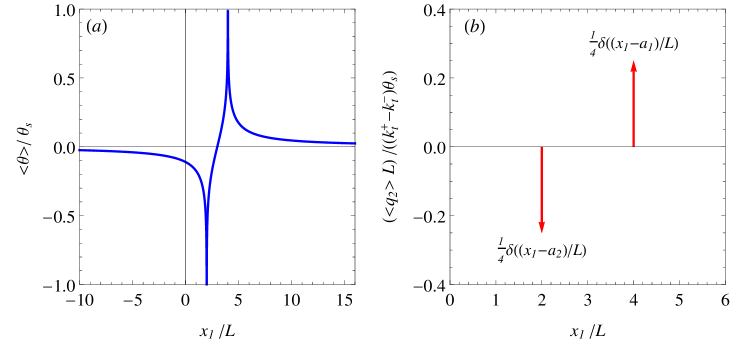
Figure 2: (a): Normalized temperature profile at the interface $x_{2}=0$ reported for $a_{1}/L=4$ and $a_{2}/L=2$; (b): Normalized average heat flux profile at the interfaces $x_{2}=0$ reported for $a_{1}/L=4$ and $a_{2}/L=2$.

For simplicity, the Dundurs parameter $d$ involved in the weight functions (88) is assumed to be zero, and then the integral identities (99) and (100) decouple and equations (99) take the form (115). Considering only the contributions due to the fluxes and temperature profiles, the uncoupled integral identities (115) become

$$\left\{\begin{array}[]{rrll}\mathcal{S}^{(s)}\cfrac{\partial[\mbox{}[u_{1}]\mbox{}]^{(-)}}{\partial x_{1}}&=&m_{t}\mathcal{S}^{(s-)}\langle\theta\rangle,&\\ &&&x_{1}<0\\ \mathcal{S}^{(s)}\cfrac{\partial[\mbox{}[u_{2}]\mbox{}]^{(-)}}{\partial x_{1}}&=&-n_{t}\langle\theta\rangle+\cfrac{h_{t}}{2}\mathcal{J}^{(s-)}\langle q_{2}\rangle+\cfrac{l_{t}}{4}\mathcal{J}^{(s-)}[\mbox{}[q_{2}]\mbox{}].\end{array}\right.$$ (120)

Remembering the definitions of $\mathcal{S}^{(s-)}$ and $\mathcal{J}^{(s-)}$ introduced in the previous Section, and applying these operators to the heat and temperature profiles (117), (118) and (119), the following results are obtained:

$$\mathcal{S}^{(s-)}\langle\theta\rangle=-\frac{\theta_{s}}{4\pi}\mathcal{S}^{(s-)}\left\{\ln\left[(x_{1}-a_{1})^{2}\right]-\ln\left[(x_{1}-a_{2})^{2}\right]\right\}=0,$$ (121)

$$\frac{h_{t}}{2}\mathcal{J}^{(s-)}\langle q_{2}\rangle+\frac{l_{t}}{4}\mathcal{J}^{(s-)}[\mbox{}[q_{2}]\mbox{}] =\frac{\theta_{s}}{8L}\varUpsilon_{t}\mathcal{J}^{(s-)}\left[\delta\left(\frac{x_{1}-a_{1}}{L}\right)-\delta\left(\frac{x_{1}-a_{2}}{L}\right)\right]$$

$$=-\frac{\theta_{s}}{8\pi}\varUpsilon_{t}\left\{\ln\left[(x_{1}-a_{1})^{2}\right]-\ln\left[(x_{1}-a_{2})^{2}\right]\right\},$$ (122)

where $\varUpsilon_{t}=l_{t}(k_{t}^{+}+k_{t}^{-})+h_{t}(k_{t}^{+}-k_{t}^{-})$, and the explicit derivation of expression (121) is reported in Appendix D.

Substituting the (121) and (122) into equations (120) we get

$$\left\{\begin{array}[]{rrll}\mathcal{S}^{(s)}\cfrac{\partial[\mbox{}[u_{1}]\mbox{}]^{(-)}}{\partial x_{1}}&=&0,&\\ &&&x_{1}<0\\ \mathcal{S}^{(s)}\cfrac{\partial[\mbox{}[u_{2}]\mbox{}]^{(-)}}{\partial x_{1}}&=&\cfrac{\theta_{s}}{4\pi}\bigg{(}n_{t}-\cfrac{\varUpsilon_{t}}{2}\bigg{)}\left\{\ln\left[(x_{1}-a_{1})^{2}\right]-\ln\left[(x_{1}-a_{2})^{2}\right]\right\}.\end{array}\right.$$ (123)

The singular integral operator $\mathcal{S}^{(s)}$ is now inverted following the procedure illustrated in Piccolroaz and Mishuris (2013) and Morini et al. (2013a). This leads to

$$\frac{\partial[\mbox{}[u_{1}]\mbox{}]^{(-)}}{\partial x_{1}} =0,$$ (124)

$$\frac{\partial[\mbox{}[u_{2}]\mbox{}]^{(-)}}{\partial x_{1}} =\frac{\theta_{s}}{\pi}\bigg{(}n_{t}-\cfrac{\varUpsilon_{t}}{2}\bigg{)}\left[-\sqrt{-\frac{a_{1}}{x_{1}}}+\sqrt{-\frac{a_{2}}{x_{1}}}+\arctan\sqrt{-\frac{a_{1}}{x_{1}}}-\arctan\sqrt{-\frac{a_{2}}{x_{1}}}\right],$$ (125)

which after integration gives explicit expressions for the crack opening associate to the heat fluxes (117) and (118) and to the temperature profiles at the interface (119):

$$[\mbox{}[u_{1}]\mbox{}]^{(-)}(x_{1}) =0,$$ (126)

$$[\mbox{}[u_{2}]\mbox{}]^{(-)}(x_{1}) =\frac{\theta_{s}}{\pi}\bigg{(}n_{t}-\cfrac{\Upsilon_{t}}{2}\bigg{)}\Bigg{[}\frac{\pi}{2}(a_{1}-a_{2})+(\sqrt{-a_{1}x_{1}}-\sqrt{-a_{2}x_{1}})$$

$$\left.+(x_{1}-a_{1})\arctan\sqrt{-\frac{a_{1}}{x_{1}}}-(x_{1}-a_{2})\arctan\sqrt{-\frac{a_{2}}{x_{1}}}\right].$$ (127)

The tractions ahead of the crack tip are given by the solution of equations (100), which in this case assume the form:

$$\left\{\begin{array}[]{rrll}\langle\sigma_{21}\rangle^{(+)}&=&-\cfrac{1}{b}\mathcal{S}^{(c)}\cfrac{\partial[\mbox{}[u_{1}]\mbox{}]^{(-)}}{\partial x_{1}}+\cfrac{m_{t}}{b}\mathcal{S}^{(s+)}\langle\theta\rangle,&\\ &&&x_{1}>0\\ \langle\sigma_{22}\rangle^{(+)}&=&-\cfrac{1}{b}\mathcal{S}^{(c)}\cfrac{\partial[\mbox{}[u_{2}]\mbox{}]^{(-)}}{\partial x_{1}}-\cfrac{n_{t}}{b}\langle\theta\rangle+\cfrac{h_{t}}{2b}\mathcal{J}^{s+)}\langle q_{2}\rangle+\cfrac{l_{t}}{4b}\mathcal{J}^{(s+)}[\mbox{}[q_{2}]\mbox{}].\end{array}\right.$$ (128)

Applying the operators $\mathcal{S}^{(s+)}$ and $\mathcal{J}^{(s+)}$ to the flux and temperature functions (117), (118) and (119), the result is given by

$$\mathcal{S}^{(s+)}\langle\theta\rangle=-\frac{\theta_{s}}{4\pi}\mathcal{S}^{(s+)}\left\{\ln\left[(x_{1}-a_{1})^{2}\right]-\ln\left[(x_{1}-a_{2})^{2}\right]\right\}=-\frac{\theta_{s}}{2}[H(a_{1}-x_{1})-H(a_{2}-x_{1})],$$ (129)

$$\frac{h_{t}}{2b}\mathcal{J}^{(s+)}\langle q_{2}\rangle+\frac{l_{t}}{4b}\mathcal{J}^{(s+)}[\mbox{}[q_{2}]\mbox{}] =\frac{\theta_{s}}{8bL}\varUpsilon_{t}\mathcal{J}^{(s+)}\left[\delta\left(\frac{x_{1}-a_{1}}{L}\right)-\delta\left(\frac{x_{1}-a_{2}}{L}\right)\right]$$

$$=-\frac{\theta_{s}}{8\pi b}\varUpsilon_{t}\left\{\ln\left[(x_{1}-a_{1})^{2}\right]-\ln\left[(x_{1}-a_{2})^{2}\right]\right\},$$ (130)

where $H(a_{1}-x_{1})$ and $H(a_{2}-x_{1})$ are Heaviside step functions (see Appendix D for details regarding the derivation of (129)). Substituting expressions (129) and (130) into equations (128), the tractions ahead of the crack tip finally become

$$\langle\sigma_{21}\rangle^{(+)}(x_{1}) =-\cfrac{m_{t}\theta_{s}}{2b}[H(a_{1}-x_{1})-H(a_{2}-x_{1})],$$ (131)

$$\langle\sigma_{22}\rangle^{(+)}(x_{1}) =-\cfrac{1}{b}\mathcal{S}^{(c)}\cfrac{\partial[\mbox{}[u_{2}]\mbox{}]^{(-)}}{\partial x_{1}}+\cfrac{\theta_{s}}{4\pi b}\bigg{(}n_{t}-\cfrac{\varUpsilon_{t}}{2}\bigg{)}\left\{\ln\left[(x_{1}-a_{1})^{2}\right]-\ln\left[(x_{1}-a_{2})^{2}\right]\right\}.$$ (132)

In order to study the influence of the different thermal expansion coefficients of the materials on the crack opening and on the tractions ahead of the tip, the upper and lower half-space media are assumed to have identical values for the elastic moduli $\lambda^{+}=\lambda^{-}=\lambda$, $\mu^{+}=\mu^{-}=\mu$, and for the thermal conductivity coefficients $k^{+}_{t}=k^{-}_{t}=k_{t}$, and dissimilar values for $\gamma_{t}$: $\gamma_{t}^{+}\neq\gamma_{t}^{-}$. in this case, the bimaterial parameters involved in expressions (127) and (132) become:

$$m_{t}=\frac{\gamma_{t}^{+}}{2(\lambda+\mu)}\bigg{(}1-\frac{\gamma_{t}^{-}}{\gamma_{t}^{+}}\Big{)}=\varXi^{+}_{t}\bigg{(}1-\frac{\gamma_{t}^{-}}{\gamma_{t}^{+}}\bigg{)},\quad n_{t}-\frac{\varUpsilon_{t}}{2}=\frac{\gamma_{t}^{+}}{2(\lambda+\mu)}\bigg{(}1+\frac{\gamma_{t}^{-}}{\gamma_{t}^{+}}\Big{)}=\varXi^{+}_{t}\bigg{(}1+\frac{\gamma_{t}^{-}}{\gamma_{t}^{+}}\bigg{)},$$

where $\varXi^{+}_{t}=\gamma_{t}^{+}/2(\lambda+\mu)$. Substituting these explicit constants in equations (127) and (132), we obtain:

$$[\mbox{}[u_{1}]\mbox{}]^{(-)}(x_{1}) =0,$$ (133)

$$[\mbox{}[u_{2}]\mbox{}]^{(-)}(x_{1}) =\frac{\theta_{s}\varXi^{+}_{t}}{\pi}\bigg{(}1+\frac{\gamma_{t}^{-}}{\gamma_{t}^{+}}\bigg{)}\Bigg{[}\frac{\pi}{2}(a_{1}-a_{2})+(\sqrt{-a_{1}x_{1}}-\sqrt{-a_{2}x_{1}})$$

$$\left.+(x_{1}-a_{1})\arctan\sqrt{-\frac{a_{1}}{x_{1}}}-(x_{1}-a_{2})\arctan\sqrt{-\frac{a_{2}}{x_{1}}}\right],$$ (134)

$$\langle\sigma_{21}\rangle^{(+)}(x_{1}) =-\cfrac{\theta_{s}\varXi^{+}_{t}}{2b}\bigg{(}1-\frac{\gamma_{t}^{-}}{\gamma_{t}^{+}}\bigg{)}[H(a_{1}-x_{1})-H(a_{2}-x_{1})],$$ (135)

$$\langle\sigma_{22}\rangle^{(+)}(x_{1}) =-\cfrac{1}{b}\mathcal{S}^{(c)}\cfrac{\partial[\mbox{}[u_{2}]\mbox{}]^{(-)}}{\partial x_{1}}+\cfrac{\theta_{s}\varXi^{+}_{t}}{4\pi b}\bigg{(}1+\frac{\gamma_{t}^{-}}{\gamma_{t}^{+}}\bigg{)}\left\{\ln\left[(x_{1}-a_{1})^{2}\right]-\ln\left[(x_{1}-a_{2})^{2}\right]\right\}.$$ (136)

Note that, as expected, for the case of homogeneous material, corresponding to $\gamma_{t}^{+}=\gamma_{t}^{-}$, $\langle\sigma_{21}\rangle^{(+)}$ vanishes indipendently of the results derived by applying the integral operators to the temperature profiles. This means that for the case of a plane crack in an homogeneous elastic themodiffusive material, no shear stresses are due to the temperature and heat flux profiles on the crack surface.

The variation of the normalized crack opening (134) is reported in Fig. 3 as a function of the spatial coordinate $x_{1}/L$ assuming a single value of the ratio $\gamma_{t}^{-}/\gamma_{t}^{+}=0.8$ and different localization of the Dirac Delta heat flux functions (117) and (118), corresponding to different values of the normalized distances $a_{1}/L$ and $a_{2}/L$. The values for these distances have been chosen such that $a_{1}>a_{2}$, as imposed in the definition of the heat flux profiles (117) and (118). The crack opening profiles shown in Fig. 3$/(a)$ have been computed considering the same value of $a_{1}/L=0.8$ and four different values of $a_{2}/L=\{0.001,0.1,1,2\}$. It can be observed that, as $a_{2}/L$ decreases, and then the contribution to the heat flux functions depending by $\delta((x_{1}-a_{2})/L)$ approaches the crack tip, the crack opening increases. In the author’s opinion, this is due to the fact that, for small values of $a_{2}/L$, the peak of the heat flux profiles (117) and (118) and the maximum of the temperature (119) are localized near to the crack tip. Consequently the maximum of the thermal load provided by these distributions of heat flux and temperature approaches the crack tip, the crack process is favored and an increase of the crack opening is produced, in analogy to what is observed for mechanical loading functions localized near to the tip (Freund, 1998).

In Fig. 3$/(b)$ the crack opening $[\mbox{}[u_{2}]\mbox{}]^{(-)}$ is reported for the same value of $a_{2}/L=2$ and four different values of $a_{1}/L=\{2.1,2.5,3,4\}$. Differently from what is detected for the variation of $a_{2}/L$, it can be noted that the crack opening becomes larger as the normalized distance $a_{1}/L$ increases. As we expect, $[\mbox{}[u_{2}]\mbox{}]^{(-)}$ is almost zero for $a_{1}/L=2.1$, since in this case $a_{1}\approx a_{2}$, and then observing expressions (117), (118) and (119) it can be easily deduced that $\left\langle q_{1}\right\rangle\approx 0$, $[\mbox{}[q_{1}]\mbox{}]\approx 0$ and $\left\langle\theta\right\rangle\approx 0$. Looking at the structure of profiles (117), (118) and (119), it can be easily deduced that if the value of $a_{2}/L$ is fixed and $a_{1}/L$ increase, the effort of the temperature and heat fluxes becomes more relevant. Consequently, the loading action provided by the temperature and the flux at the interface increases and gives rise to higher values of the crack opening.

The variation of the normalized traction $\langle\sigma_{22}\rangle^{(+)}$ is plotted in Fig. 4 as a function of the spatial coordinate $x_{1}/L$ for the same single value of the ratio $\gamma_{t}^{-}/\gamma_{t}^{+}=0.8$ and the same sets of values of $a_{1}/L$ and $a_{2}/L$ assumed for the crack opening. In order to compute profiles of the traction $\langle\sigma_{22}\rangle^{(+)}$, the symbolic computation program Mathematica was used. As it can be expected, the tractions exhibit a singular behaviour at the crack tip, for $x_{1}=0$, and for $x_{1}=a_{1}$ and $x_{1}=a_{2}$, where the temperature profile (119) diverges.

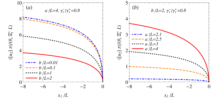
Figure 3: (a): Variation of the normalized crack opening $[\mbox{}[u_{2}]\mbox{}]^{(-)}$ with the spatial coordinate $x_{1}/L$, reported for different values of $a_{1}/L$; (b): Variation of the normalized crack opening $[\mbox{}[u_{2}]\mbox{}]^{(-)}$ with the spatial coordinate $x_{1}/L$, reported for different values of $a_{2}/L$.

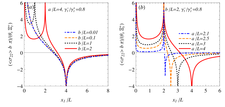
Figure 4: (a): Variation of the normalized traction $\langle\sigma_{22}\rangle^{(+)}$ with the spatial coordinate $x_{1}/L$, reported for different values of $a_{1}/L$; (b): Variation of the normalized traction $\langle\sigma_{22}\rangle^{(+)}$ with the spatial coordinate $x_{1}/L$, reported for different values of $a_{2}/L$.

In Fig. 5 the crack opening $[\mbox{}[u_{2}]\mbox{}]^{(-)}$ and the traction ahead of the tip are reported as functions of $x_{1}/L$ for single values of $a_{1}/L=4$ and of $a_{2}/L=2$ and several values of the ratio $\gamma_{t}^{-}/\gamma_{t}^{+}=\{0.8,1.2,1,0.8\}$. It can be noted that greater values of $\gamma_{t}^{-}/\gamma_{t}^{+}$ correspond to a greater crack opening. This means that, taking into account the considered heat flux, the temperature profiles and the geometry of the model, the crack process is favored if the thermal expansion coefficient of the material occupying the lower half-space is greater with respect to that of the medium occupying the upper half-plane.

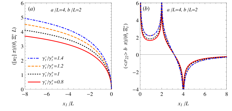
Figure 5: (a): Variation of the normalized crack opening $[\mbox{}[u_{2}]\mbox{}]^{(-)}$ with the spatial coordinate $x_{1}/L$, reported for different values of the ratio $\gamma_{t}^{-}/\gamma_{t}^{+}$; (b): Variation of the normalized traction $\langle\sigma_{22}\rangle^{(+)}$ with the spatial coordinate $x_{1}/L$, reported for different values of the ratio $\gamma_{t}^{-}/\gamma_{t}^{+}$.

The traction expressions (136) can now be used for calculating the stress intensity factors. Applying the standard definition reported in Freund (1998), we obtain

$$K_{I} =\lim_{x_{1}\rightarrow 0}\sqrt{2\pi x_{1}}\langle\sigma_{22}\rangle^{(+)}(x_{1})=\frac{3\sqrt{2\pi}\theta_{s}\varXi^{+}_{t}}{b}\bigg{(}1+\frac{\gamma_{t}^{-}}{\gamma_{t}^{+}}\bigg{)}\bigg{(}\sqrt{\frac{a_{1}}{L}}-\sqrt{\frac{a_{2}}{L}}\bigg{)},$$ (137)

$$K_{II} =\lim_{x_{1}\rightarrow 0}\sqrt{2\pi x_{1}}\langle\sigma_{21}\rangle^{(+)}(x_{1})=0.$$ (138)

In Fig. 6$/(a)$ the variation of the normalized stress intensity factor $K_{I}$ with the ratio $a_{2}/L$ is reported for $a_{1}/L=4$ and several values the ratio $\gamma_{t}^{-}/\gamma_{t}^{+}=\{0.8,1.2,1,0.8\}$. It can be observed that $K_{I}=0$ for $a_{2}/L=a_{1}/L=4$. This is due to the fact that for $a_{2}/L=a_{1}/L$ both the heat flux and temperature profiles vanish (see expressions (117), (118) and (119)), and consequently no thermal load is present at the interface and no crack opening is generated. Moreover, it can be noted that as $a_{2}/L$ decreases, $K_{I}$ increases monotonically. This behaviour is in agreement with what is detected analysing the crack opening, and also in this case it can be explained observing that for small values of $a_{2}/L$ the heat flux profiles (117) and (118) and the temperature (119) possess a peak localized at the crack tip. As a consequence, the maximum of the provided thermal load approaches the crack tip and the crack process is favored. In Fig. 6$/(b)$, $K_{I}$ is plotted as a function of $a_{1}/L$ assuming $a_{2}/L=2$ and the same values $\gamma_{t}^{-}/\gamma_{t}^{+}=\{0.8,1.2,1,0.8\}$. According to what is observed in Fig. 6$/(a)$, $K_{I}=0$ for $a_{2}/L=a_{1}/L=2$. The reported curves show that the stress intensity factor becomes larger as $a_{1}/L$ increases. This behaviour is due to the characteristics of the heat flux and temperature expressions (117), (118) and (119): looking at the structure of these profiles, it can be easily verified that if the value of $a_{2}/L$ is fixed and$a_{1}/L$, the effort of temperature and heat fluxes becomes more relevant, then the loading action provided by thermal effects increases. Consequently, the crack process is favored and the value of $K_{I}$ becomes larger as does the crack opening (see Fig. 3$/(b)$). Observing both Fig. 6$/(a)$ and Fig. 6$/(b)$, it can be noted that the stress intensity factor increases as the ratio $\gamma_{t}^{-}/\gamma_{t}^{+}$. This confirms the behaviour detected observing the crack opening, and it means that considering the heat flux and temperature profiles given by expressions (117), (118) and (119), the crack process is favored if the thermal expansion coefficient of the material occupying the lower half-plane is greater with respect to that of the medium occupying the upper half-plane.

Considering the case of a homogeneous material, where we have $\gamma_{t}^{-}=\gamma_{t}^{+}=\gamma_{t}$, the crack opening (134) assume the form

$$[\mbox{}[u_{1}]\mbox{}]^{(-)}(x_{1}) =0,$$ (139)

$$[\mbox{}[u_{2}]\mbox{}]^{(-)}(x_{1}) =\frac{\gamma_{t}\theta_{s}}{\pi(\lambda+\mu)}\Bigg{[}\frac{\pi}{2}(a_{1}-a_{2})+(\sqrt{-a_{1}x_{1}}-\sqrt{-a_{2}x_{1}})$$

$$\left.+(x_{1}-a_{1})\arctan\sqrt{-\frac{a_{1}}{x_{1}}}-(x_{1}-a_{2})\arctan\sqrt{-\frac{a_{2}}{x_{1}}}\right],$$ (140)

and then the tractions ahead of the tip (136) become

$$\langle\sigma_{21}\rangle^{(+)}(x_{1}) =0,$$ (141)

$$\langle\sigma_{22}\rangle^{(+)}(x_{1}) =-\cfrac{1}{b}\mathcal{S}^{(c)}\cfrac{\partial[\mbox{}[u_{2}]\mbox{}]^{(-)}}{\partial x_{1}}+\cfrac{\mu\gamma_{t}\theta_{s}}{4\pi(\lambda+2\mu)}\left\{\ln\left[(x_{1}-a_{1})^{2}\right]-\ln\left[(x_{1}-a_{2})^{2}\right]\right\},$$ (142)

where

$$\cfrac{1}{b}\frac{\partial[\mbox{}[u_{2}]\mbox{}]^{(-)}}{\partial x_{1}}=\cfrac{\mu\gamma_{t}\theta_{s}}{\pi(\lambda+2\mu)}\left[-\sqrt{-\frac{a_{1}}{x_{1}}}+\sqrt{-\frac{a_{2}}{x_{1}}}+\arctan\sqrt{-\frac{a_{1}}{x_{1}}}-\arctan\sqrt{-\frac{a_{2}}{x_{1}}}\right].$$ (143)

Expressions (140), (142) and (143) can be easily obtained deriving the Green’s function corresponding to a thermoelastic semi-plane with the punctually localized fluxes (117) and (118) applied on the boundary.

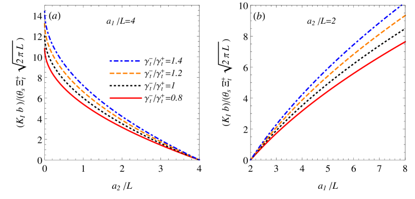
Figure 6: (a): Variation of the normalized stress intensity factor $K_{I}$ with the ratio $a_{2}/L$, reported for $a_{1}/L=2$ and assuming different values of $\gamma_{t}^{-}/\gamma_{t}^{+}$; (b): Variation of the normalized stress intensity factor $K_{I}$ with the ratio $a_{1}/L$, reported for $a_{2}/L=2$ and assuming different values of the ratio $\gamma_{t}^{-}/\gamma_{t}^{+}$.

5.2 Symmetrically distributed temperature profile at the interface

The following distribution profile for the avegare temperature across the plane $x_{2}=0$, containing both the crack and the interface, is considered:

$$\left\langle\theta\right\rangle(x_{1})=\frac{\theta_{s}x_{1}}{L}e^{-\frac{x_{1}^{2}}{L^{2}}}.$$ (144)

The temperature is assumed to be continous at the interface, then $[\mbox{}[\theta]\mbox{}](x_{1})=0$ for $-\infty<x_{1}<+\infty$. The average and the jump of the normal heat flux $q_{2}$ at the interface corresponding to the average temperature profile (144) and to the assumption $[\mbox{}[\theta]\mbox{}](x_{1})=0$ has been evaluated solving the steady state heat conduction equation for both the upper and the lower thermodiffusive half-space. This procedure is reported details in Appendix C.2, and the resulting average and jump of the of the noramal heat flux are given by

$$\left\langle q_{2}\right\rangle(x_{1})=-(k_{t}^{+}-k_{t}^{-})\frac{\theta_{s}}{L}\left[\left(\frac{2x_{1}^{2}}{L^{2}}-1\right)e^{-\frac{x_{1}^{2}}{L^{2}}}\mbox{Erfi}\left(\frac{x_{1}}{L}\right)-\frac{2x_{1}}{L\sqrt{\pi}}\right],$$ (145)

$$[\mbox{}[q_{1}]\mbox{}](x_{1})=-2(k_{t}^{+}+k_{t}^{-})\frac{\theta_{s}}{L}\left[\left(\frac{2x_{1}^{2}}{L^{2}}-1\right)e^{-\frac{x_{1}^{2}}{L^{2}}}\mbox{Erfi}\left(\frac{x_{1}}{L}\right)-\frac{2x_{1}}{L\sqrt{\pi}}\right].$$ (146)

It can be easily verified that the normal heat flux profiles (145) and (146) satisfy the integral balance conditions introduced in Section 3. The variation of the normalized average temperature (144) and of the normalized average heat flux (145) is plotted as a function of the spatial coordinate $x_{1}/L$ in Fig. 7.

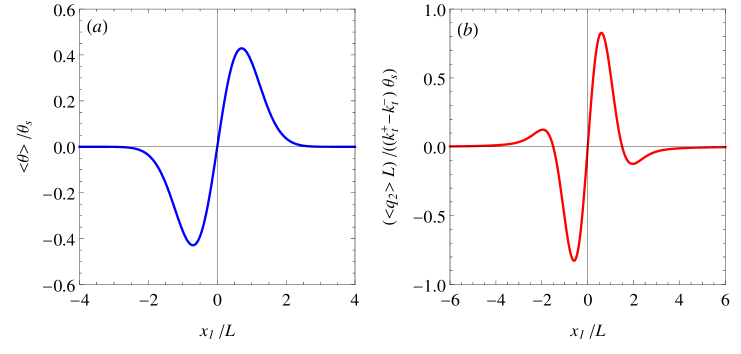
Figure 7: (a): Normalized temperature profile at the interface $x_{2}=0$; (b): Normalized average heat flux profile at the interfaces $x_{2}=0$.

Also for this example, the Dundurs parameter $d$ involved in the weight functions (88) is assumed to be zero, and then considering the contributions due to the fluxes and temperature profiles, the uncoupled integral identities have the form (120). Applying the integral operator $\mathcal{J}^{(s-)}$ to the average and jump of the normal heat flux (145) and (146), the following result is obtained

$$\frac{h_{t}}{2}\mathcal{J}^{(s-)}\langle q_{2}\rangle+\frac{l_{t}}{4}\mathcal{J}^{(s-)}[\mbox{}[q_{2}]\mbox{}]=\frac{\theta_{s}\varUpsilon_{t}x_{1}}{2L}e^{-\frac{x_{1}^{2}}{L^{2}}}.$$ (147)

Substituting expression (147) into equations (120), we get

$$\left\{\begin{array}[]{rrll}\mathcal{S}^{(s)}\cfrac{\partial[\mbox{}[u_{1}]\mbox{}]^{(-)}}{\partial x_{1}}&=&m_{t}\theta_{s}\mathcal{S}^{(s-)}\bigg{(}\cfrac{x_{1}}{L}e^{-\frac{x_{1}^{2}}{L^{2}}}\bigg{)},&\\ &&&x_{1}<0\\ \mathcal{S}^{(s)}\cfrac{\partial[\mbox{}[u_{2}]\mbox{}]^{(-)}}{\partial x_{1}}&=&-\theta_{s}\bigg{(}n_{t}-\cfrac{\varUpsilon_{t}}{2}\bigg{)}\cfrac{x_{1}}{L}e^{-\frac{x_{1}^{2}}{L^{2}}}\end{array}\right.,$$ (148)

where $\varUpsilon_{t}$ is the same bimaterial parameter defined in Section 5.1. Using the procedure reported in Piccolroaz and Mishuris (2013) and Morini et al. (2013a), the singular integral operator $\mathcal{S}^{(s)}$ can be inverted. This leads to

$$\frac{\partial[\mbox{}[u_{1}]\mbox{}]^{(-)}}{\partial x_{1}} =m_{t}\theta_{s}\mathcal{S}^{(s)-1}\mathcal{S}^{(s-)}\bigg{(}\cfrac{x_{1}}{L}e^{-\frac{x_{1}^{2}}{L^{2}}}\bigg{)},$$ (149)

$$\frac{\partial[\mbox{}[u_{2}]\mbox{}]^{(-)}}{\partial x_{1}} =-\theta_{s}\bigg{(}n_{t}-\cfrac{\varUpsilon_{t}}{2}\bigg{)}\mathcal{S}^{(s)-1}\bigg{(}\cfrac{x_{1}}{L}e^{-\frac{x_{1}^{2}}{L^{2}}}\bigg{)}.$$ (150)

The results provided by the application of the operators $\mathcal{S}^{(s)-1}$ and $\mathcal{S}^{(s-)}$ to the function $(x_{1}/L)\cdot e^{-\frac{x_{1}^{2}}{L^{2}}}$ are calculated by means of the symbolic computation program Mathematica. The crack opening $[\mbox{}[u_{1}]\mbox{}]^{(-)}$ and $[\mbox{}[u_{2}]\mbox{}]^{(-)}$ are derived by integrating respectively expressions (149) and (150).

Applying the operators $\mathcal{S}^{(s+)}$ to the flux functions (145) and (146), the following result is derived

$$\frac{h_{t}}{2}\mathcal{J}^{(s+)}\langle q_{2}\rangle+\frac{l_{t}}{4}\mathcal{J}^{(s+)}[\mbox{}[q_{2}]\mbox{}]=\frac{\theta_{s}\Upsilon_{t}x_{1}}{2L}e^{-\frac{x_{1}^{2}}{L^{2}}}.$$ (151)

Substituting expression (151) into equations (128), the tractions ahead of the crack tip become

$$\langle\sigma_{21}\rangle^{(+)}(x_{1}) =\cfrac{m_{t}\theta_{s}}{b}\bigg{[}\mathcal{S}^{(s+)}\bigg{(}\cfrac{x_{1}}{L}e^{-\frac{x_{1}^{2}}{L^{2}}}\bigg{)}-\mathcal{S}^{(c)}\mathcal{S}^{(s)-1}\mathcal{S}^{(s-)}\bigg{(}\cfrac{x_{1}}{L}e^{-\frac{x_{1}^{2}}{L^{2}}}\bigg{)}\bigg{]},$$ (152)

$$\langle\sigma_{22}\rangle^{(+)}(x_{1}) =-\cfrac{\theta_{s}}{b}\bigg{(}n_{t}-\cfrac{\varUpsilon_{t}}{2}\bigg{)}\bigg{[}\cfrac{x_{1}}{L}e^{-\frac{x_{1}^{2}}{L^{2}}}-\mathcal{S}^{(c)}\mathcal{S}^{(s)-1}\bigg{(}\cfrac{x_{1}}{L}e^{-\frac{x_{1}^{2}}{L^{2}}}\bigg{)}\bigg{]}.$$ (153)

Also for the example described in this Section, the upper and lower half-space media are assumed to have identical values for the elastic moduli $\lambda^{+}=\lambda^{-}=\lambda$, $\mu^{+}=\mu^{-}=\mu$, and for the thermal conductivity coefficients $k^{+}_{t}=k^{-}_{t}=k_{t}$, and dissimilar values for $\gamma_{t}$: $\gamma_{t}^{+}\neq\gamma_{t}^{-}$. In this case, the equations (149) and (150) become

$$\frac{\partial[\mbox{}[u_{1}]\mbox{}]^{(-)}}{\partial x_{1}} =\theta_{s}\varXi_{t}^{+}\bigg{(}1-\frac{\gamma_{t}^{-}}{\gamma_{t}^{+}}\bigg{)}\mathcal{S}^{(s)-1}\mathcal{S}^{(s-)}\bigg{(}\cfrac{x_{1}}{L}e^{-\frac{x_{1}^{2}}{L^{2}}}\bigg{)},$$ (154)

$$\frac{\partial[\mbox{}[u_{2}]\mbox{}]^{(-)}}{\partial x_{1}} =-\theta_{s}\varXi_{t}^{+}\bigg{(}1+\frac{\gamma_{t}^{-}}{\gamma_{t}^{+}}\bigg{)}\mathcal{S}^{(s)-1}\bigg{(}\cfrac{x_{1}}{L}e^{-\frac{x_{1}^{2}}{L^{2}}}\bigg{)},$$ (155)

and the expressions (152) and (153) assume the form

$$\langle\sigma_{21}\rangle^{(+)}(x_{1}) =\cfrac{\theta_{s}\varXi_{t}^{+}}{b}\bigg{(}1-\frac{\gamma_{t}^{-}}{\gamma_{t}^{+}}\bigg{)}\bigg{[}\mathcal{S}^{(s+)}\bigg{(}\cfrac{x_{1}}{L}e^{-\frac{x_{1}^{2}}{L^{2}}}\bigg{)}-\mathcal{S}^{(c)}\mathcal{S}^{(s)-1}\mathcal{S}^{(s-)}\bigg{(}\cfrac{x_{1}}{L}e^{-\frac{x_{1}^{2}}{L^{2}}}\bigg{)}\bigg{]},$$ (156)

$$\langle\sigma_{22}\rangle^{(+)}(x_{1}) =-\cfrac{\theta_{s}\varXi_{t}^{+}}{b}\bigg{(}1+\frac{\gamma_{t}^{-}}{\gamma_{t}^{+}}\bigg{)}\bigg{[}\cfrac{x_{1}}{L}e^{-\frac{x_{1}^{2}}{L^{2}}}-\mathcal{S}^{(c)}\mathcal{S}^{(s)-1}\bigg{(}\cfrac{x_{1}}{L}e^{-\frac{x_{1}^{2}}{L^{2}}}\bigg{)}\bigg{]},$$ (157)

where the quantity $\varXi_{t}^{+}$ is the same defined in Section 5.1.

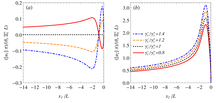
Figure 8: (a): Variation of the normalized crack opening $[\mbox{}[u_{1}]\mbox{}]^{(-)}$ with the spatial coordinate $x_{1}/L$, reported for different values of the ratio $\gamma_{t}^{-}/\gamma_{t}^{+}$; (b): Variation of the normalized crack opening $[\mbox{}[u_{2}]\mbox{}]^{(-)}$ with the spatial coordinate $x_{1}/L$, reported for different values of the ratio $\gamma_{t}^{-}/\gamma_{t}^{+}$.

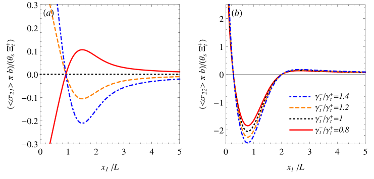
Figure 9: (a): Variation of the normalized traction $\langle\sigma_{21}\rangle^{(+)}$ with the spatial coordinate $x_{1}/L$, reported for different values of the ratio $\gamma_{t}^{-}/\gamma_{t}^{+}$; (b): Variation of the normalized crack traction $\langle\sigma_{22}\rangle^{(+)}$ with the spatial coordinate $x_{1}/L$, reported for different values of the ratio $\gamma_{t}^{-}/\gamma_{t}^{+}$.

The normalized profiles of the crack opening components $[\mbox{}[u_{1}]\mbox{}]^{(-)}$ and $[\mbox{}[u_{2}]\mbox{}]^{(-)}$, obtained by integrating expressions (154) and (155), are reported in Fig. 8 as function of $x_{1}/L$. Four different values of the ratio $\gamma_{t}^{-}/\gamma_{t}^{+}=\{0.8,1.2,1,0.8\}$ were considered for the computations. For $\gamma_{t}^{-}/\gamma_{t}^{+}=1$, corresponding to the case of an homogeneous material, we have $[\mbox{}[u_{1}]\mbox{}]^{(-)}=0$. This behaviour can be directly deduced observing expression (154). Observing Fig. 8$/(a)$, it can be noted that the crack opening component $[\mbox{}[u_{1}]\mbox{}]^{(-)}$ changes sign at a determinate distance $x_{1}^{*}/L$ from the crack tip. As it is shown in the figure, this distance is independent of the ratio $\gamma_{t}^{-}/\gamma_{t}^{+}$, it then varies with the value of $a/L$ and $b/L$. For $\gamma_{t}^{-}/\gamma_{t}^{+}>1$, $[\mbox{}[u_{1}]\mbox{}]^{(-)}$ is positive near to the crack tip, and then becomes negative for $x_{1}/L<x_{1}^{*}/L$. This means that, if $\gamma_{t}^{-}>\gamma_{t}^{+}$, in the $x_{1}-$direction, associated with the propagation Mode II, the crack opens for $x_{1}/L>x_{1}^{*}/L$ and closes for $x_{1}/L<x_{1}^{*}/L$. The opposite behaviour is shown for $\gamma_{t}^{-}/\gamma_{t}^{+}<1$, corresponding to a crack opening for $x_{1}/L<x_{1}^{*}/L$ and to a crack closing for $x_{1}/L>x_{1}^{*}/L$, near to the tip. Conversely, the component $[\mbox{}[u_{2}]\mbox{}]^{(-)}$ illustrated in Fig. 8$/(b)$ is positive everywhere for any value of $\gamma_{t}^{-}/\gamma_{t}^{+}$. It follows that in the $x_{2}-$direction, corresponding to the propagation Mode I we have crack opening for any value of the thermal expansion coefficients of the materials.

The variation of the normalized tractions $\langle\sigma_{21}\rangle^{(+)}$ and $\langle\sigma_{22}\rangle^{(+)}$ is plotted in Fig. 9 as a function of the spatial coordinate $x_{1}/L$ for the same values of $\gamma_{t}^{-}/\gamma_{t}^{+}$ assumed for the crack opening. In order to compute the integrals involved in equations (156) and (157) the symbolic computation program Mathematica was used. It can be observed that both $\langle\sigma_{21}\rangle^{(+)}$ and $\langle\sigma_{22}\rangle^{(+)}$ exhibit a singular behaviour at the crack tip, for $x_{1}=0$. This behaviour is associated with the leading term of the asymptotic expansion of expressions (156) and (157) for $x_{1}/L\rightarrow 0$, corresponding respectively to the thermal stress intensity factors $K_{t}^{II}$ and $K_{t}^{I}$ (Liu and Kardomateas, 2005).

Also in this case, exact expressions for the stress intensity factors can be evaluated by means of the tractions (156) and (157). Applying the standard definition reported in Freund (1998), we obtain

$$K_{I} =\lim_{x_{1}\rightarrow 0}\sqrt{2\pi x_{1}}\langle\sigma_{22}\rangle^{(+)}(x_{1})=\frac{3\pi^{3/2}\sqrt{L}\theta_{s}\varXi^{+}_{t}}{4b}\bigg{(}1+\frac{\gamma_{t}^{-}}{\gamma_{t}^{+}}\bigg{)}\left(\frac{\Gamma(3/4)}{\Gamma(1/4)\Gamma(7/4)}\right),$$ (158)

$$K_{II} =\lim_{x_{1}\rightarrow 0}\sqrt{2\pi x_{1}}\langle\sigma_{21}\rangle^{(+)}(x_{1})=-\frac{\pi^{3/2}\sqrt{L}\theta_{s}\varXi^{+}_{t}}{b\Gamma(1/4)}\bigg{(}1-\frac{\gamma_{t}^{-}}{\gamma_{t}^{+}}\bigg{)}.$$ (159)

6 Conclusions

The problem of a quasi-static semi-infinite interfacial crack between two dissimilar thermodiffusive elastic materials has been formulated in terms of boundary integral equations by means of Betti’s reciprocity identity and weight functions. For the case of a plane strain crack, explicit integral identities relating the applied mechanical loading, the temperature, mass density, heat and mass flux distributions at the interface and the resulting crack opening have been obtained. The solution of this system of singular integral equations provides explicit expressions for the crack opening and the stress fields associate to any arbitrary harmonic temperature and mass density profile and self-balanced heat or mass flux distribution at the interface.

Illustrative examples of the application of the integral identities to crack problems characterized by punctually localized and distributed heat flux profiles on the interface were performed. The crack opening and tractions ahead of the tip corresponding to the assumed temperature and heat flux distributions were derived by analytical inversion of the singular integral operators. In addition, exact expressions for the stress intensity factors were obtained.

The proposed original method provides a general boundary integral formulation for interfacial crack problems in thermodiffusive bimaterials avoiding the use of the Green’s function and the related challenging numerical calculations. The integral identities can be applied for studying the effects of any harmonic temperature and mass concentration profile as well as of any self-balanced heat and mass flux distributions on crack opening and traction fields ahead of the tip. This approach can have various relevant applications, expecially in the modelling of fracture processes induced by thermal and diffusive stresses at the interface between different components of mutlti-layered electrochemical devices such as solid oxide fuel cells and lithium ions batteries. Moreover, the derived integral identities have their own value from the mathematical point of view, because, to the authors best knowledge, a similar explicit formulation in terms of singular integral equations seems to be unknown in the literature.

Appendix A Bimaterial parameters

In this Appendix we report explicit expressions for the bimaterial parameters defined in Sections 2 and 3. The parameters $b,d,\gamma$ and $\alpha$ contained in the weight functions matrices (88) are the same as defined in Piccolroaz et al. (2009), here expressed in function of $\lambda,\mu$ instead of $\nu,\mu$:

$$b=\frac{\lambda^{+}+2\mu^{+}}{2\mu^{+}(\lambda^{+}+\mu^{+})}+\frac{\lambda^{-}+2\mu^{-}}{2\mu^{-}(\lambda^{-}+\mu^{-})},\quad d=\frac{1}{2(\lambda^{+}+\mu^{+})}-\frac{1}{2(\lambda^{-}+\mu^{-})},$$ (160)

$$\alpha=\frac{\mu^{-}(\lambda^{-}+\mu^{-})(\lambda^{+}+2\mu^{+})-\mu^{+}(\lambda^{+}+\lambda^{+})(\lambda^{-}+2\mu^{-})}{\mu^{-}(\lambda^{-}+\mu^{-})(\lambda^{+}+2\mu^{+})+\mu^{+}(\lambda^{+}+\lambda^{+})(\lambda^{-}+2\mu^{-})},$$ (161)

$$\gamma=\frac{\mu^{+}\mu^{-}(\lambda^{-}+\mu^{-})+\mu^{+}\mu^{-}(\lambda^{+}+\mu^{+})}{\mu^{-}(\lambda^{+}+2\mu^{+})(\lambda^{-}+\mu^{-})+\mu^{+}(\lambda^{-}+2\mu^{-})(\lambda^{+}+\mu^{+})}.$$ (162)

The bimaterial parameters associated with the effects of the temperature and heat diffusion are given by:

$$h_{t}=\frac{\gamma_{t}^{+}}{4k_{t}^{+}\mu^{+}}-\frac{\gamma_{t}^{-}}{4k_{t}^{-}\mu^{-}},\quad\ell_{t}=\frac{\gamma_{t}^{+}}{4k_{t}^{+}\mu^{+}}+\frac{\gamma_{t}^{-}}{4k_{t}^{-}\mu^{-}},$$ (163)

$$m_{t}=\frac{\gamma_{t}^{+}}{2(\lambda^{+}+\mu^{+})}-\frac{\gamma_{t}^{-}}{2(\lambda^{-}+\mu^{-})},\quad n_{t}=\frac{\gamma_{t}^{+}(\lambda^{+}+3\mu^{+})}{4\mu^{+}(\lambda^{+}+\mu^{+})}+\frac{\gamma_{t}^{-}(\lambda^{-}+3\mu^{-})}{4\mu^{-}(\lambda^{-}+\mu^{-})},$$ (164)

$$p_{t}=\frac{\gamma_{t}^{+}}{2(\lambda^{+}+\mu^{+})}+\frac{\gamma_{t}^{-}}{2(\lambda^{-}+\mu^{-})},\quad q_{t}=\frac{\gamma_{t}^{+}(\lambda^{+}+3\mu^{+})}{4\mu^{+}(\lambda^{+}+\mu^{+})}-\frac{\gamma_{t}^{-}(\lambda^{-}+3\mu^{-})}{4\mu^{-}(\lambda^{-}+\mu^{-})},$$ (165)

and the constant corresponding to the concentration and the mass diffusion presents the following form:

$$h_{c}=\frac{\gamma_{c}^{+}}{4D_{c}^{+}\mu^{+}}-\frac{\gamma_{c}^{-}}{4D_{c}^{-}\mu^{-}},\quad\ell_{c}=\frac{\gamma_{c}^{+}}{4D_{c}^{+}\mu^{+}}+\frac{\gamma_{c}^{-}}{4D_{c}^{-}\mu^{-}},$$ (166)

$$m_{c}=\frac{\gamma_{c}^{+}}{2(\lambda^{+}+\mu^{+})}-\frac{\gamma_{c}^{-}}{2(\lambda^{-}+\mu^{-})},\quad n_{c}=\frac{\gamma_{c}^{+}(\lambda^{+}+3\mu^{+})}{4\mu^{+}(\lambda^{+}+\mu^{+})}+\frac{\gamma_{c}^{-}(\lambda^{-}+3\mu^{-})}{4\mu^{-}(\lambda^{-}+\mu^{-})},$$ (167)

$$p_{c}=\frac{\gamma_{c}^{+}}{2(\lambda^{+}+\mu^{+})}+\frac{\gamma_{c}^{-}}{2(\lambda^{-}+\mu^{-})},\quad q_{c}=\frac{\gamma_{c}^{+}(\lambda^{+}+3\mu^{+})}{4\mu^{+}(\lambda^{+}+\mu^{+})}-\frac{\gamma_{c}^{-}(\lambda^{-}+3\mu^{-})}{4\mu^{-}(\lambda^{-}+\mu^{-})}.$$ (168)

Appendix B Elastic potentials in weight functions space

In this Appendix, the derivation of the explicit expressions for the Fourier transform of the elastic potentials (LABEL:PhiPsiexpl) is explained in details. These expressions are given by the solution of the ODEs system (57), which is shown here

$$\left\{\begin{array}[]{c}\tilde{\varPsi}^{{}^{\prime}}-i\xi\tilde{\varPhi}=\tilde{U}_{1}\\ \tilde{\varPhi}^{{}^{\prime}}+i\xi\tilde{\varPsi}=\tilde{U}_{2}\end{array}\right.,$$ (169)

where considering the upper half-plane $x_{1}>0$, the non-homgeneous terms in the system (169) are given by the weight functions

$$\tilde{U}_{1}(\xi,x_{2}) = \left\{\left[x_{2}-\frac{\lambda^{+}+2\mu^{+}}{|\xi|(\lambda^{+}+\mu^{+})}\right]\tilde{\varSigma}_{21}^{-}+i\left[\frac{\mu^{+}}{\xi(\lambda^{+}+\mu^{+})}-\mathop{\mathrm{sign}}(\xi)x_{2}\right]\tilde{\varSigma}_{22}^{-}\right\}\frac{e^{-|\xi|x_{2}}}{2\mu^{+}},$$

$$\tilde{U}_{2}(\xi,x_{2}) = \left\{-i\left[\mathop{\mathrm{sign}}(\xi)x_{2}+\frac{\mu^{+}}{\xi(\lambda^{+}+\mu^{+})}\right]\tilde{\varSigma}_{21}^{-}-\left[x_{2}+\frac{\lambda^{+}+2\mu^{+}}{|\xi|(\lambda^{+}+\mu^{+})}\right]\tilde{\varSigma}_{22}^{-}\right\}\frac{e^{-|\xi|x_{2}}}{2\mu^{+}}.$$

The ODEs system (169) can be rewritten in the matrix form:

$$\mbox{\boldmath$y$}^{{}^{\prime}}+\mbox{\boldmath$Q$}\mbox{\boldmath$y$}=\mbox{\boldmath$c$},$$ (171)

where $\mbox{\boldmath$y$}=[\tilde{\varPsi},\tilde{\varPhi}]^{T}$, $\mbox{\boldmath$c$}=[\tilde{U}_{1},\tilde{U}_{2}]^{T}$ and

$$\mbox{\boldmath$Q$}=\left[\begin{array}[]{cc}0&-i\xi\\ i\xi&0\end{array}\right].$$ (172)

The eigenvectors and the eigenvalues of the matrix (172) are now defined:

$$(\mbox{\boldmath$Q$}-\lambda\mbox{\boldmath$I$})\mbox{\boldmath$w$}=0.$$ (173)

The eigeinvalues are easily determined by solving the characteristic equation:

$$\mbox{det}(\mbox{\boldmath$Q$}-\lambda\mbox{\boldmath$I$})=\lambda^{2}-\xi^{2}=0,\quad\Rightarrow\quad\lambda_{1}=|\xi|,\lambda_{2}=-|\xi|,$$ (174)

then the eigenvector matrix $\mbox{\boldmath$W$}=(\mbox{\boldmath$w$}_{1},\mbox{\boldmath$w$}_{2})^{T}$ and its inverse are given by

$$\mbox{\boldmath$W$}=\left[\begin{array}[]{cc}i\mathop{\mathrm{sign}}(\xi)&-i\mathop{\mathrm{sign}}(\xi)\\ 1&1\end{array}\right],\quad\mbox{\boldmath$W$}^{-1}=\frac{1}{2}\left[\begin{array}[]{cc}-i\mathop{\mathrm{sign}}(\xi)&1\\ i\mathop{\mathrm{sign}}(\xi)&1\end{array}\right],$$ (175)

Applying the standard eigenvalues method and using the matrices (175) the system (171) is written in the following equivalent form

$$\mbox{\boldmath$z$}^{{}^{\prime}}+\mbox{\boldmath$W$}^{-1}\mbox{\boldmath$Q$}\mbox{\boldmath$W$}\mbox{\boldmath$z$}=\mbox{\boldmath$d$},$$ (176)

where $\mbox{\boldmath$z$}=\mbox{\boldmath$W$}^{-1}\mbox{\boldmath$y$}$, $\mbox{\boldmath$d$}=\mbox{\boldmath$W$}^{-1}\mbox{\boldmath$c$}$ and

$$\mbox{\boldmath$W$}^{-1}\mbox{\boldmath$Q$}\mbox{\boldmath$W$}=\left[\begin{array}[]{cc}|\xi|&0\\ 0&-|\xi|\end{array}\right].$$ (177)

The (176) consists of two decoupled equations:

$$\left\{\begin{array}[]{c}z_{1}^{{}^{\prime}}-|\xi|z_{1}=d_{1}\\ z_{2}^{{}^{\prime}}+|\xi|z_{2}=d_{2}\end{array}\right.,$$ (178)

where the non-homogeneous terms $\mbox{\boldmath$d$}=\mbox{\boldmath$W$}^{-1}\mbox{\boldmath$c$}$ are given by

$$d_{1}=-\frac{1}{2}[i\mathop{\mathrm{sign}}(\xi)\tilde{U}_{1}-\tilde{U}_{2}],\quad d_{1}=\frac{1}{2}[i\mathop{\mathrm{sign}}(\xi)\tilde{U}_{1}+\tilde{U}_{2}].$$ (179)

The general solutions of equations (178) assume the form

$$z_{1}(\xi,x_{2}) = C_{1}e^{|\xi|x_{2}}-\left[ix_{2}\tilde{\varSigma}_{21}^{-}+\left(\mathop{\mathrm{sign}}(\xi)x_{2}+\frac{1}{\xi}\right)\tilde{\varSigma}_{22}^{-}\right]\frac{e^{-|\xi|x_{2}}}{4\xi\mu^{+}},$$

$$z_{2}(\xi,x_{2}) = C_{2}e^{-|\xi|x_{2}}+\left(i\mathop{\mathrm{sign}}(\xi)\tilde{\varSigma}_{21}^{-}+\tilde{\varSigma}_{22}^{-}\right)\frac{(\lambda^{+}+3\mu^{+})x_{2}e^{-|\xi|x_{2}}}{4|\xi|(\lambda^{+}+\mu^{+})\mu^{+}}.$$

Assuming that the displacements and the stresses vanish for $x_{1}\rightarrow+\infty$, the following condition must be imposed: $C_{1}=0$. The expressions for the transformed elastic potentials $\mbox{\boldmath$y$}=\mbox{\boldmath$W$}\mbox{\boldmath$z$}=[\tilde{\varPsi},\tilde{\varPhi}]^{T}$ in the upper half-plane can then be obtained by means of the following relations:

$$\tilde{\varPsi}=i\mathop{\mathrm{sign}}(\xi)(z_{1}-z_{2}),\quad\tilde{\varPhi}=z_{1}+z_{2}.$$ (181)

Substituting expressions (B) in equations (181), we get:

$$\tilde{\varPhi}(\xi,x_{2}) = C_{2}e^{-|\xi|x_{2}}+\left\{-i\frac{x_{2}\mu^{+}}{\xi(\lambda^{+}+\mu^{+})}\tilde{\varSigma}_{21}^{-}+\left[\frac{1}{2\xi^{2}}-\frac{x_{2}\mu^{+}}{|\xi|(\lambda^{+}+\mu^{+})}\right]\tilde{\varSigma}_{22}^{-}\right\}\frac{e^{-|\xi|x_{2}}}{2\mu^{+}},$$

$$\tilde{\varPsi}(\xi,x_{2}) = i\mathop{\mathrm{sign}}(\xi)C_{2}e^{-|\xi|x_{2}}+\left\{-\frac{x_{2}(\lambda^{+}+2\mu^{+})}{|\xi|(\lambda^{+}+\mu^{+})}\tilde{\varSigma}_{21}^{-}+i\left[\frac{\mathop{\mathrm{sign}}(\xi)}{2\xi^{2}}+\frac{x_{2}(\lambda^{+}+2\mu^{+})}{\xi(\lambda^{+}+\mu^{+})}\right]\tilde{\varSigma}_{22}^{-}\right\}\frac{e^{-|\xi|x_{2}}}{2\mu^{+}}.$$

assuming $C_{2}=0$, the expressions (LABEL:PhiPsiexpl) are finally derived. Similarly to the case of the displacements, replacing $-|\xi|$ with $|\xi|$, $\mu^{+}$ with $\mu^{-}$ and $\lambda^{+}$ with $\lambda^{-}$ in the (LABEL:PhiPsiapp) the elastic potentials for the lower half-plane are obtained.

Appendix C Temperature and heat flux profiles

The temperature and heat flux profiles used in Section 5 are now derived by solving the heat transmission problem in a semi-plane for different sets of boundary conditions. Considering the upper thermodiffusive half-plane $x_{1}>0$, the temperature profile $\theta^{+}(x_{1},x_{2})$ is given by the solution of the two-dimensional Laplace’s equation

$$\Delta\theta^{+}=0,\quad x_{2}>0,$$ (183)

Two different sets of boundary conditions are considered for the solution of equation (183).

C.1 Punctually localized heat flux profile at the interface

The following profile for the temperature on the boundary $x_{2}=0^{+}$ is assumed

$$q_{2}^{+}(x_{1},x_{2}=0^{+})=\frac{\theta_{s}k_{t}^{+}}{2L}\left[\delta\left(\frac{x_{1}-a_{1}}{L}\right)-\delta\left(\frac{x_{1}-a_{2}}{L}\right)\right],$$ (184)

where $a_{1},a_{2},L>0$ and $a_{1}>a_{2}$. It is easy to verify that the flux function (184) satisfies the self-balance condition (36)₍₁₎. Substituting expression (184) into the heat flux definition (6)₍₁₎ and remembering the condition (35)₍₁₎, the following boundary conditions are defined for the the temperature function $\theta^{+}$

$$\theta^{+}(x_{1},x_{2}=+\infty)=0,\qquad\left.\frac{\partial\theta^{+}}{\partial x_{2}}\right|_{x_{2}=0^{+}}=-\frac{\theta_{s}}{2L}\left[\delta\left(\frac{x_{1}-a_{1}}{L}\right)-\delta\left(\frac{x_{1}-a_{2}}{L}\right)\right].$$ (185)

Applying the Fourier transform with respect to the variable $x_{1}$, the equation (183) becomes

$$\tilde{\theta}^{+^{\prime\prime}}-\xi^{2}\tilde{\theta}^{+}=0,$$ (186)

where ${}^{{}^{\prime}}$ denotes the derivative with respect to $x_{2}$. The general solution of equation (186) takes the form

$$\tilde{\theta}^{+}(\xi,x_{2})=C_{1}e^{-|\xi|x_{2}}+C_{2}e^{|\xi|x_{2}},$$ (187)

where the constants $C_{1}$ and $C_{2}$ are determined by boundary conditions (185). They are given by

$$C_{1}=\frac{\theta_{s}}{2|\xi|}(e^{ia_{1}\xi}-e^{-ia_{2}\xi}),\qquad C_{2}=0,$$ (188)

consequently, the Fourier transform of the temperature profile for this case becomes

$$\tilde{\theta}^{+}(\xi,x_{2})=\frac{\theta_{s}}{2|\xi|}(e^{ia_{1}\xi}-e^{-ia_{2}\xi})e^{-|\xi|x_{2}},$$ (189)

and the temperature $\theta^{+}$ is obtained applying the Fourier inversion to expression (189)

$$\theta^{+}(x_{1},x_{2})=-\frac{\theta_{s}}{4\pi}\left\{\ln\left[(x_{1}-a_{1})^{2}+x_{2}^{2}\right]-\ln\left[(x_{1}-a_{2})^{2}+x_{2}^{2}\right]\right\}.$$ (190)

Assuming the same profile (184) for the normal heat flux on the boundary $x_{2}=0^{-}$, an expression similar to the (190) is derived for the temperature $\theta^{-}$ in the lower half-plane $x_{2}<0$. The average and the jump of the temperature across the plane $x_{2}=0$, which are defined respectively by expressions (30)₍₁₎ and (31)₍₁₎, are then given by

$$\left\langle\theta\right\rangle(x_{1})=-\frac{\theta_{s}}{4\pi}\left[\ln(x_{1}-a_{1})^{2}-\ln(x_{1}-a_{2})^{2}\right],\quad[\mbox{}[\theta]\mbox{}](x_{1})=0,$$ (191)

and the average and jump of the normal heat flux, defined by expressions (33)₍₁₎ and (34)₍₁₎, finally become

$$\left\langle q_{1}\right\rangle(x_{1})=\frac{\theta_{s}}{4L}(k_{t}^{+}-k_{t}^{-})\left[\delta\left(\frac{x_{1}-a_{1}}{L}\right)-\delta\left(\frac{x_{1}-a_{2}}{L}\right)\right],$$ (192)

$$[\mbox{}[q_{1}]\mbox{}](x_{1})=\frac{\theta_{s}}{2L}(k_{t}^{+}+k_{t}^{-})\left[\delta\left(\frac{x_{1}-a_{1}}{L}\right)-\delta\left(\frac{x_{1}-a_{2}}{L}\right)\right].$$ (193)

C.2 Symmetrically distributed temperature profile at the interface

The following distributed profile for the temperature on the boundary $x_{2}=0^{+}$ is assumed

$$\theta^{+}(x_{1},x_{2}=0^{+})=\frac{\theta_{s}x_{1}}{L}e^{-\frac{x_{1}^{2}}{L^{2}}}.$$ (194)

The boundary conditions for the temperature $\theta^{+}(x_{1},x_{2})$ are given by expression (194) together with the relation (35)₍₁₎ here reported

$$\theta^{+}(x_{1},x_{2}=+\infty)=0.$$ (195)

Also in this case, the Fourier transform of the temperature $\tilde{\theta}^{+}(\xi,x_{2})$ is given by the solution of equation (186), and then it takes the form (187). The constants $C_{1}$ and $C_{2}$, determined by means of boundary conditions (194) and (195), become

$$C_{1}=\frac{i\sqrt{\pi}\theta_{s}L^{2}}{2}\xi e^{-\frac{L^{2}\xi^{2}}{4}},\qquad C_{2}=0,$$ (196)

and then the Fourier transform of the temperature profile is given by

$$\tilde{\theta}^{+}(\xi,x_{2})=\frac{i\sqrt{\pi}\theta_{s}L^{2}}{2}\xi e^{-\left(|\xi|x_{2}+\frac{L^{2}\xi^{2}}{4}\right)}.$$ (197)

Applying the inverse Fourier transform to (197), the following profile for the temperature in the upper half-plane is derived

$$\theta^{+}(x_{1},x_{2})=\frac{\theta_{s}}{2}e^{-\frac{x_{1}^{2}-x_{2}^{2}}{L^{2}}}\left\{x_{1}\cos\left(\frac{2x_{1}x_{2}}{L^{2}}\right)+x_{2}\sin\left(\frac{2x_{1}x_{2}}{L^{2}}\right)\right.$$

$$\left.-x_{1}\mathop{\mathrm{Im}}\left[e^{-\frac{2ix_{1}x_{2}}{L^{2}}}\mbox{Erfi}\left(\frac{x_{1}+ix_{2}}{L}\right)\right]-x_{2}\mathop{\mathrm{Re}}\left[e^{-\frac{2ix_{1}x_{2}}{L^{2}}}\mbox{Erfi}\left(\frac{x_{1}+ix_{2}}{L}\right)\right]\right\}.$$ (198)

Assuming the same profile (194) for the temperature on the boundary $x_{2}=0^{-}$, the following expression is derived for the temperature $\theta^{-}$ in the lower half-plane $x_{2}<0$:

$$\theta^{-}(x_{1},x_{2})=\frac{\theta_{s}}{2}e^{-\frac{x_{1}^{2}-x_{2}^{2}}{L^{2}}}\left\{x_{1}\cos\left(\frac{2x_{1}x_{2}}{L^{2}}\right)+x_{2}\sin\left(\frac{2x_{1}x_{2}}{L^{2}}\right)\right.$$

$$\left.+x_{1}\mathop{\mathrm{Im}}\left[e^{-\frac{2ix_{1}x_{2}}{L^{2}}}\mbox{Erfi}\left(\frac{x_{1}+ix_{2}}{L}\right)\right]+x_{2}\mathop{\mathrm{Re}}\left[e^{-\frac{2ix_{1}x_{2}}{L^{2}}}\mbox{Erfi}\left(\frac{x_{1}+ix_{2}}{L}\right)\right]\right\}.$$ (199)

The average and the jump of the temperature across the plane $x_{2}=0$ containing both the crack and the interface are then given by

$$\left\langle\theta\right\rangle(x_{1})=\frac{\theta_{s}x_{1}}{L}e^{-\frac{x_{1}^{2}}{L^{2}}},\quad[\mbox{}[\theta]\mbox{}](x_{1})=0,$$ (200)

and the average and the jump of the normal heat flux finally become

$$\left\langle q_{2}\right\rangle(x_{1})=-(k_{t}^{+}-k_{t}^{-})\frac{\theta_{s}}{L}\left[\left(\frac{2x_{1}^{2}}{L^{2}}-1\right)e^{-\frac{x_{1}^{2}}{L^{2}}}\mbox{Erfi}\left(\frac{x_{1}}{L}\right)-\frac{2x_{1}}{L\sqrt{\pi}}\right],$$ (201)

$$[\mbox{}[q_{1}]\mbox{}](x_{1})=-2(k_{t}^{+}+k_{t}^{-})\frac{\theta_{s}}{L}\left[\left(\frac{2x_{1}^{2}}{L^{2}}-1\right)e^{-\frac{x_{1}^{2}}{L^{2}}}\mbox{Erfi}\left(\frac{x_{1}}{L}\right)-\frac{2x_{1}}{L\sqrt{\pi}}\right].$$ (202)

It can be easily verified that flux profiles (201) and (202) satisfy the integral balance conditions.

Appendix D Evaluation of integrals $\mathcal{S}^{(s-)}$ and $\mathcal{S}^{(s+)}$ for logarithmic functions

In this Appendix the explicit derivation of results (121) and (129) is reported in detail. Assuming that the temperature profile at the interface is given by expression (119) and applying the operator $\mathcal{S}^{(s-)}$ the following integral expression is obtained

$$\mathcal{S}^{(s-)}\langle\theta\rangle =-\frac{\theta_{s}}{4\pi}\mathcal{S}^{(s-)}\left\{\ln\left[(x_{1}-a_{1})^{2}\right]-\ln\left[(x_{1}-a_{2})^{2}\right]\right\}$$

$$=-\frac{\theta_{s}}{4\pi^{2}}\bigg{\{}\int_{-\infty}^{+\infty}\frac{\ln[(t-a_{1})^{2}]}{x_{1}-t}dt-\int_{-\infty}^{+\infty}\frac{\ln[(t-a_{2})^{2}]}{x_{1}-t}dt\bigg{\}}$$

$$=-\frac{\theta_{s}}{4\pi^{2}}[I_{1}^{-}(x_{1})-I_{2}^{-}(x_{1})],\qquad x_{1}<0,\ a_{1},a_{2}>0,\ a_{1}>a_{2}.$$ (203)

In order to evaluate $I_{1}^{-}$, a change of variables is operated

$$w=t-a_{1},\ \ dw=dt,\ \ x_{1}-t=h-w,\ \ h=x_{1}-a_{1},\quad\mbox{where}\ a_{1}>0,\ x_{1}<0,\ \Rightarrow\ h<0,$$

and then this term becomes

$$I_{1}^{-}(x_{1})=I_{1}^{-}(h)=\mathcal{P}\int_{-\infty}^{+\infty}\frac{\ln[w^{2}]}{h-w}dw=\pi^{2},\qquad h<0.$$ (204)

Similarly, for calculating $I_{2}^{-}$ the following change of variables is introduced

$$s=t-a_{2},\ \ ds=dt,\ \ x_{1}-t=\ell-s,\ \ \ell=x_{1}-a_{2},\quad\mbox{where}\ a_{2}>0,\ x_{1}<0\ \Rightarrow\ \ell<0,$$

and this lead to

$$I_{2}^{-}(x_{1})=I_{2}^{-}(\ell)=\mathcal{P}\int_{-\infty}^{+\infty}\frac{\ln[s^{2}]}{\ell-s}ds=\pi^{2},\qquad\ell<0.$$ (205)

As a consequence, substituting the (204) and (205) into equation (203), it can be observed that the final result coincides with expression (121) introduced in Section 5.1

$$\mathcal{S}^{(s-)}\langle\theta\rangle=-\frac{\theta}{4\pi^{2}}[I_{1}^{-}(h)-I_{2}^{-}(\ell)]=0,\qquad\forall h,\ell<0.$$ (206)

Applying the operator $\mathcal{S}^{(s+)}$ to the temperature profile (119), an integral expression analogous to (203) is derived

$$\mathcal{S}^{(s+)}\langle\theta\rangle =-\frac{\theta_{s}}{4\pi}\mathcal{S}^{(s+)}\left\{\ln\left[(x_{1}-a_{1})^{2}\right]-\ln\left[(x_{1}-a_{2})^{2}\right]\right\}$$

$$=-\frac{\theta_{s}}{4\pi^{2}}\bigg{\{}\int_{-\infty}^{+\infty}\frac{\ln[(t-a_{1})^{2}]}{x_{1}-t}dt-\int_{-\infty}^{+\infty}\frac{\ln[(t-a_{2})^{2}]}{x_{1}-t}dt\bigg{\}}$$

$$=-\frac{\theta_{s}}{4\pi^{2}}[I_{1}^{+}(x_{1})-I_{2}^{+}(x_{1})],\qquad x_{1}>0,\ a_{1},a_{2}>0,\ a_{1}>a_{2}.$$ (207)

In order to calculate $I_{1}^{+}$, a change of variable identical to that operated for evaluating $I_{1}^{-}$ is defined

$$w=t-a_{1},\ \ dw=dt,\ \ x_{1}-t=h-w,\ \ h=x_{1}-a_{1},\quad\mbox{where}\ a_{1}>0,\ x_{1}>0.$$

It is important to note that, differently from the term $I_{1}^{-}$, characterized by $h<0$, for the evaluation of $I_{1}^{+}$ both the cases $h<0$ and $h>0$ must be considered. Consequently the result is given by

$$I_{1}^{+}(x_{1})=I_{1}^{+}(h)=\mathcal{P}\int_{-\infty}^{+\infty}\frac{\ln[w^{2}]}{h-w}dw=\left\{\begin{array}[]{cc}\pi^{2}&h<0,\ \Rightarrow\ x_{1}<a_{1},\\ -\pi^{2}&h>0,\ \Rightarrow\ x_{1}>a_{1},\end{array}\right.$$ (208)

Similarly, for calculating $I_{2}^{+}$ the same change of variable used for $I_{2}^{-}$ is introduced

$$s=t-a_{2},\ \ ds=dt,\ \ x_{1}-t=\ell-s,\ \ \ell=x_{1}-a_{2},\quad\mbox{where}\ a_{2}>0,\ x_{1}>0,$$

and the result of the integral is given by

$$I_{2}^{+}(x_{1})=I_{2}^{+}(\ell)=\mathcal{P}\int_{-\infty}^{+\infty}\frac{\ln[s^{2}]}{\ell-s}ds=\left\{\begin{array}[]{cc}\pi^{2}&\ell<0,\ \Rightarrow\ x_{1}<a_{2},\\ -\pi^{2}&\ell>0,\ \Rightarrow\ x_{1}>a_{2},\end{array}\right.$$ (209)

The sum of the terms (208) and (209) becomes

$$I_{1}^{+}(h)-I_{2}^{+}(\ell)=\left\{\begin{array}[]{cl}0&h<0,\ \ell<0,\ \Rightarrow 0<x_{1}<a_{2},\\ 2\pi^{2}&h<0,\ \ell>0,\ \Rightarrow a_{2}<x_{1}<a_{1},\\ 0&h>0,\ \ell>0,\ \Rightarrow x_{1}>a_{1},\end{array}\right.$$

and then substituting this expression into equation (207) the following final result is obtained

$$\mathcal{S}^{(s+)}\langle\theta\rangle=\left\{\begin{array}[]{cl}0&0<x_{1}<a_{2},\\ -\cfrac{\theta_{s}}{2}&a_{2}<x_{1}<a_{1},\\ 0&x_{1}>a_{1},\end{array}\right.$$ (210)

The equation (210) can be expressed by introducing the Heaviside functions $H(a_{1}-x_{1})$ and $H(a_{2}-x_{1})$ (Arfken and Weber, 2005), and then it becomes identical to the (129) used in Section 5.1

$$\mathcal{S}^{(s+)}\langle\theta\rangle=-\frac{\theta_{s}}{2}[H(a_{1}-x_{1})-H(a_{2}-x_{1})],\qquad a_{1}>a_{2}.$$ (211)

References

- Anandakumar et al. (2010) Anandakumar, G., Li, N., Verma, A., Singh, P., Kim, J.-H., 2010. Thermal stress and probability of failure analyses of functionally graded solid oxide fuel cells. J. Power Sources 195, 6659–6670.
- Ang and Telles (2004) Ang, W. T., Telles, J. C. F., 2004. A numerical Green’s function for multiple cracks in anisotropic bodies. J. Eng. Math. 49, 197–207.
- Arfken and Weber (2005) Arfken, G. B., Weber, H. J., 2005. Mathematical methods for physicists, 5th edition. Elsevier Academic Press, San Diego.
- Bigoni and Capuani (2002) Bigoni, D., Capuani, D., 2002. Green’s function for incremental nonlinear elasticity: shear bands and boundary integral formulation. J. Mech. Phys. Solids 50, 471–500.
- Brebbia et al. (1984) Brebbia, C. A., Telles, J. C. F., Wrobel, L. C., 1984. Boundary Element Techniques. Springer-Verlag, Berlin.
- Brychkov and Prudnikov (1989) Brychkov, Y. A., Prudnikov, A. P., 1989. Integral transforms of generalized functions. Gordon and Breach.
- Budiansky and Rice (1979) Budiansky, B., Rice, J. R., 1979. An integral equation for dynamic elastic response of an isolated 3-D crack. Wave Motion 1, 187–192.
- Bueckner (1985) Bueckner, H. F., 1985. Weight functions and fundamental fields for the penny-shaped and the half plane crack in three-space. Int. J. Solids Struct. 23, 57–93.
- Bueckner (1989) Bueckner, H. F., 1989. Observations on weight functions. Eng. Anal. Bound. Elem. 6, 3–18.
- Cheng et al. (2001) Cheng, A. H.-D., Chen, C. S., Golberg, M. A., Rashed, Y. F., 2001. BEM for thermoelasticity and elasticity with body force-a revisit. Eng. Anal. Boundary Elem. 25, 377–387.
- Dell’Erba et al. (1998) Dell’Erba, D. N., Aliabadi, M. H., Rooke, D. P., 1998. Dual boudary element method for three-dimensional thermoelastic crack problems. Int. J. Fract. 94, 89–101.
- Freund (1998) Freund, L. B., 1998. Dynamic Fracture Mechanics. Cambridge University Press.
- Gakhov and Cherski (1978) Gakhov, F. D., Cherski, Y. I., 1978. Equations of the convolutions type. Nauka, Moscow.
- Gohberg and Krein (1958) Gohberg, I., Krein, M. G., 1958. Systems of integral equations on an half line with kernels depending on the difference of arguments. Uspekhi Mat. Nauk. 13, 3–72.
- Goutianos et al. (2010) Goutianos, S., Frandsen, H. L., Sorensen, B. F., 2010. Fracture properties of nickel-based anodes for solid oxide fuel cells. J. Eur. Cer. Soc. 30, 3173–3179.
- Hou et al. (2008) Hou, P.-F., Leung, A. Y. T., He, Y.-J., 2008. Three-dimensional Green’s function for transversely isotropic thermoelastic bimaterials. Int. J. Solids Struct. 45, 6659–6670.
- Krein (1958) Krein, M. G., 1958. Integral equations on an half-line with kernels depending upon the difference of the arguments. Uspekhi Mat. Nauk. 13, 73–120.
- Kumar and Chawla (2012a) Kumar, R., Chawla, V., 2012a. General steady-state solution and Green’s function in orthotropic piezothermoelastic diffusion medium. Arch. Mech. 64, 555—579.
- Kumar and Chawla (2012b) Kumar, R., Chawla, V., 2012b. Green’s functions in orthotropic thermoelastic diffusion media. Eng. Anal. Bound. Elem. 36, 1272–1277.
- Linkov et al. (1997) Linkov, A. M., Zubkov, V. V., Kheib, M. A., 1997. A method of solving three-dimensional problems of seam working and geological faults. J. Min. Sci. 33, 295–315.
- Liu and Kardomateas (2005) Liu, L., Kardomateas, G. A., 2005. Thermal stress intensity factors for a crack in an anisotropic half plane. Int. J. Solids Struct. 42, 5208–5223.
- Lowrie and Rawlings (2000) Lowrie, F. L., Rawlings, R. D., 2000. Room and high temperature failure mechanisms in solid oxide fuel cell electrolytes. J. Eur. Cer. Soc. 20, 751–760.
- Malzbender et al. (2003) Malzbender, J., Steinbrech, R. W., Singheiser, L., 2003. Determination of the interfacial fracture energies of cathodes and glass ceramic sealants in a planar solid-oxide fuel cell design. J. Mat. Res. 18, 929–934.
- Mishuris et al. (2014) Mishuris, G., Piccolroaz, A., Vellender, A., 2014. Boundary integral formulation for cracks at imperfect interfaces. Quat. J. Mech. Appl. Math. 67, 363–387.
- Morini et al. (2013a) Morini, L., Piccolroaz, A., Mishuris, G., Radi, E., 2013a. Integral identities for a semi-infinite interfacial crack in anisotropic elastic bimaterials. Int. J. Solids Struct. 50, 1437–1448.
- Morini et al. (2013b) Morini, L., Radi, E., Movchan, A. B., Movchan, N. V., 2013b. Stroh formalism in analysis of skew-symmetric and symmetric weight functions for interfacial cracks. Math. Mech. Solids 18, 135–152.
- Nowacki (1974a) Nowacki, W., 1974a. Dynamical problems of thermodiffusion in solids. I. Bull. Polish Acad. Sci. Tech. Sci. 22, 55–64.
- Nowacki (1974b) Nowacki, W., 1974b. Dynamical problems of thermodiffusion in solids. II. Bull. Polish Acad. Sci. Tech. Sci. 22, 205–211.
- Pharr et al. (2013) Pharr, M., Vlassak, J. J., Suo, Z., 2013. Measurements of fracture energy of lithiated silicon electrodes for Li-Ion batteries. Nano Lett. 13, 5570–5577.
- Piccolroaz and Mishuris (2013) Piccolroaz, A., Mishuris, G., 2013. Integral identities for a semi-infinite interfacial crack in 2D and 3D elasticity. J. Elasticity 110, 117–140.
- Piccolroaz et al. (2009) Piccolroaz, A., Mishuris, G., Movchan, A. B., 2009. Symmetric and skew symmetric weight functions in 2D perturbation models for semi-infinite interfacial cracks. J. Mech. Phys. Solids 57, 1657–1682.
- Rice (1968) Rice, J., 1968. Mathematical analysis in the mechanics of fracture. In: Fracture: And advanced treatise. Vol. 1. Academic Press, San Diego, pp. 191–311.
- Rizzo and Shippy (1977) Rizzo, F. J., Shippy, D. J., 1977. An advanced boundary integral equation method for three-dimensional elasticity. Int. J. Num. Methods Eng. 11, 1753–1768.
- Roos (1969) Roos, B. W., 1969. Analitic functions and distributions in physics and engeneering. Wiley, New York.
- Sherief et al. (2004) Sherief, H. H., Hamza, F. A., Saleh, H. A., 2004. The theory of generalized thermoelastic diffusion. Int. J. Eng. Sci. 42, 591–608.
- Shiah and Tan (1999) Shiah, Y. C., Tan, C. L., 1999. Exact integral transformation of the thermoelastic domain integral in BEM for general 2D anisotropic elasticity. Comp. Mech. 23, 87–96.
- Shiah and Tan (2012) Shiah, Y. C., Tan, C. L., 2012. Boundary element method for thermoelastic analysis of three-dimensionnal transversely isotropic solids. Int. J. Solids Struct. 49, 2924–2933.
- Sladek and Sladek (1983) Sladek, V., Sladek, J., 1983. Boundary integral equation method in thermoelasticity part I: general analysis. Appl. Math. Modelling 7, 241–253.
- Sladek and Sladek (1984a) Sladek, V., Sladek, J., 1984a. Boundary integral equation method in thermoelasticity part II: crack analysis. Appl. Math. Modelling 8, 27–36.
- Sladek and Sladek (1984b) Sladek, V., Sladek, J., 1984b. Boundary integral equation method in thermoelasticity part III: uncoupled thermoelasticity. Appl. Math. Modelling 8, 413–418.
- Slaughter (2001) Slaughter, W. S., 2001. The Linearized Theory of Elasticity. Birkhuser, Boston.
- Sturla and Barber (1988) Sturla, F. A., Barber, J. R., 1988. Thermoelastic Green’s functions for plane problems in general anisotropy. ASME J. Appl. Mech. 55, 245–247.
- Vekua (1970) Vekua, N. P., 1970. Systems of singular integral equations. Nauka, Moscow.
- Vellender et al. (2013) Vellender, A., Mishuris, G., Piccolroaz, A., 2013. Perturbation analysis for an imperfect interface crack problem using weight function techniques. Int. J. Solids Struct. 50, 4098–4107.
- Weaver (1977) Weaver, J., 1977. Three-dimensional crack analysis. Int. J. Solids Struct. 13, 321–330.
- Willis and Movchan (1995) Willis, J. R., Movchan, A. B., 1995. Dynamic weight function for a moving crack. I. Mode I loading. J. Mech. Phys. Solids 43, 319–341.
- Zhang et al. (2010) Zhang, J., Lu, B., Song, Y., Xiang, J., 2010. Diffusion induced stress in layered Li-ion battery electrode plates. J. Power Sources 209, 220–227.
- Zhao et al. (2010) Zhao, K., Pharr, M., Vlassak, J. J., Suo, Z., 2010. Fracture of electrodes in lithium-ion batteries caused by fast charging. J. Appl. Phys. 108, 073517.