On the universal structure of human lexical semantics

Abstract

How universal is human conceptual structure? The way concepts are organized in the human brain may reflect distinct features of cultural, historical, and environmental background in addition to properties universal to human cognition. Semantics, or meaning expressed through language, provides direct access to the underlying conceptual structure, but meaning is notoriously difficult to measure, let alone parameterize. Here we provide an empirical measure of semantic proximity between concepts using cross-linguistic dictionaries. Across languages carefully selected from a phylogenetically and geographically stratified sample of genera, translations of words reveal cases where a particular language uses a single polysemous word to express concepts represented by distinct words in another. We use the frequency of polysemies linking two concepts as a measure of their semantic proximity, and represent the pattern of such linkages by a weighted network. This network is highly uneven and fragmented: certain concepts are far more prone to polysemy than others, and there emerge naturally interpretable clusters loosely connected to each other. Statistical analysis shows such structural properties are consistent across different language groups, largely independent of geography, environment, and literacy. It is therefore possible to conclude the conceptual structure connecting basic vocabulary studied is primarily due to universal features of human cognition and language use.

The space of concepts expressible in any language is vast. This space is covered by individual words representing semantically tight neighborhoods of salient concepts. There has been much debate about whether semantic similarity of concepts is shared across languages Whorf1956 ; Fodor1975 ; Wierzbicka1996 ; Lucy1992 ; Levinson2003 ; ChoiBowerman1991 ; Majid2008 ; Croft2010 . On the one hand, all human beings belong to a single species characterized by, among other things, a shared set of cognitive abilities. On the other hand, the 6000 or so extant human languages spoken by different societies in different environments across the globe are extremely diverse EvansLevinson2009 ; Comrie1989 ; Croft2003 and may reflect accidents of history as well as adaptations to local environments. Most psychological experiments about this question have been conducted on members of “WEIRD” (Western, Educated, Industrial, Rich, Democratic) societies, yet there is reason to question whether the results of such research are valid across all types of societies Henrich2010 . Thus, the question of the degree to which conceptual structures expressed in language are due to universal properties of human cognition, the particulars of cultural history, or the environment inhabited by a society, remains unresolved.

The search for an answer to this question has been hampered by a major methodological difficulty. Linguistic meaning is an abstract construct that needs to be inferred indirectly from observations, and hence is extremely difficult to measure; this is even more apparent in the field of lexical semantics. Meaning thus contrasts both with phonetics, in which instrumental measurement of physical properties of articulation and acoustics is relatively straightforward, and with grammatical structure, for which there is general agreement on a number of basic units of analysis Shopen2007 . Much lexical semantic analysis relies on linguists’ introspection, and the multifaceted dimensions of meaning currently lack a formal characterization. To address our primary question, it is necessary to develop an empirical method to characterize the space of lexical meanings.

We arrive at such a measure by noting that translations uncover the alternate ways that languages partition meanings into words. Many words have more than one meaning, or sense, to the extent that word senses can be individuated CroftCruse2004 . Words gain meanings when their use is extended by speakers to similar meanings; words lose meanings when another word is extended to the first word’s meaning, and the first word is replaced in that meaning. To the extent that words in transition across similar, or possibly contiguous, meanings account for the polysemy (multiple meanings of a single word form) revealed in cross-language translations, the frequency of polysemies found across an unbiased sample of languages can provide a measure of semantic similarity among word meanings. The unbiased sample of languages is carefully chosen in a phylogenetically and geographically stratified way, according to the methods of typology and universals research Comrie1989 ; Croft2003 . This large, diverse sample of languages allows us to avoid the pitfalls of research based solely on “WEIRD” societies and to separate contributions to the empirically attested patterns in the linguistic data, arising from universal language cognition versus those from artifacts of the speaker-groups’ history or way of life.

There have been several cross-linguistic surveys of lexical polysemy, and its potential for understanding semantic shift Koptjevskaja2012 , in the domains such as body parts Brown1976 ; WitkowskiBrown1978 , cardinal directions Brown1983 , perception verbs Viberg1983 , concepts associated with fire Evans1992 , and color metaphors Derrig1978 . We add a new dimension to the existing body of research by providing a comprehensive mathematical method using a systematically stratified global sample of languages to measure degrees of similarity. Our cross-linguistic study takes the Swadesh lists as basic concepts Swadesh1952 as most languages have words for them. Among those concepts, we chose 22 meanings associated with two domains: celestial objects (e.g. SUN, MOON, STAR) and landscape objects (e.g. FIRE, WATER, MOUNTAIN, DUST). For each word expressing one of these meanings, we examined what other concepts were also expressed by the word. Since the semantic structures of these two domains are very likely to be influenced by the physical environment that human societies inhabit, any claim of universality of lexical semantics needs to be demonstrated here.

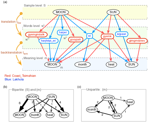
Figure 1: Schematic figure of the construction of network representations. (a) Tripartite polysemy network constructed through translation (links from the first to the second layer) and back-translation (links from the second to the third layer) for the cases of MOON and SUN in two American languages: Coast Tsimshian (red links) and Lakhota (blue links). (b) Directed bipartite graph of two languages grouped, projected from the tripartite graph above by aggregating links in the second layer. (c) Directed and weighted unipartite graph, projected from the bipartite graph by identifying and merging the same Swadesh words (MOON and SUN in this case).

Results

We represent word-meaning and meaning-meaning relations uncovered by translation dictionaries between each language in the unbiased sample and major modern European languages by constructing a network structure. Two meanings (represented by a set of English words) are linked if they are translated from one to another and then back, and the link is weighted by the number of paths of the translation, or the number of words that represent both meanings (see Methods for detail). Figure 1 illustrates the construction in the case of two languages, Lakhota (primarily spoken in North and South Dakota) and Coast Tsimshian (mostly spoken in northwestern British Columbia and southeastern Alaska). Translation of SUN in Lakhota results wí and á$\eta$pawí. While the later picks up no other meaning, wí is a polysemy that possesses additional meanings of MOON and month, hence they are linked to SUN. Such polysemy is also observed in Coast Tsimshian where gyemk, translated from SUN, covers additional meanings including, thus additionally linking to, heat.

Each language has its own way of partitioning meanings by words, captured in a semantic network of the language. It is conceivable, however, that a group of languages bear structural resemblance perhaps because the speakers share historical or environmental features. A link between SUN and MOON, for example, reoccurs in both languages, but does not appear in many other languages. SUN is instead linked to divinity and time in Japanese, and to thirst and DAY/DAYTIME in !Xóõ. The question then is the degree to which the observed polysemy patterns are general or sensitive to the environment inhabited by the speech community, phylogenetic history of the languages, and intrinsic linguistic factors such as literary tradition. We test such question by grouping the individual networks in a number of ways according to properties of their corresponding languages. We first analyze the networks of the entire languages, and then of sub-groups.

In Fig. 2, we present the network of the entire languages exhibiting the broad topological structure of polysemies observed in our data. It reveals three almost-disconnected clusters, groups of concepts that are indeed more prone to polysemy within, that are associated with a natural semantic interpretation. The semantically most uniform cluster, colored in blue, includes concepts related to water. A second, smaller cluster, colored in yellow, associates solid natural substances (centered around STONE/ROCK) with their topographic manifestation (MOUNTAIN). The third cluster, in red, is more loosely connected, bridging a terrestrial cluster and a celestial cluster, including less tangible substances such as WIND, SKY, and FIRE, and salient time intervals such as DAY and YEAR. In keeping with many traditional oppositions between EARTH and SKY/heaven, or darkness, and light, the celestial, and terrestrial components form two sub-clusters connected most strongly through CLOUD, which shares properties of both. The result reveals a coherent set of relationships among concepts that possibly reflects human cognitive conceptualization of these semantic domains Croft2003 ; Croft2010 ; Vygotsky:thought_lang:02 .

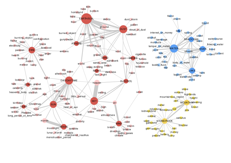
Figure 2: Connectance graph of concepts. Concepts are connected through polysemous words that cover the concepts. Swadesh entries are capitalized. Links whose weights are more than two are presented, and direction is omitted for simplicity. The size of a node and the width of a link to another node are proportional to the number of polysemies associated with the concept, and with the two connected concepts, respectively. The thick link from SKY to heaven denotes the large number of polysemies across languages. Three distinct clusters are identified and coloured by red, blue, and yellow, which may imply a coherent set of relationship among concepts that possibly reflects human cognitive conceptualization of these semantic domains.

We test whether these relationships are universal rather than particular to properties of linguistic groups such as physical environment that human societies inhabit. We first categorized languages by nonlinguistic variables such as geography, topography, climate, and the existence or nonexistence of a literary tradition (Table 2 in Appendix) and constructed a network for each group. A spectral algorithm then clusters Swadesh entries into a hierarchical structure or dendrogram for each language group. Using standard metrics on trees Critchlow:96 ; Dobson:75 ; Robinson-Foulds , we find that the dendrograms of language groups are much closer to each other than to dendrograms of randomly permuted leaves: thus the hypothesis that languages of different subgroups share no semantic structure in common is rejected ($p<0.05$, see Methods)—SEA/OCEAN and SALT are, for example, more related than either is to SUN in every group we tried. In addition, the distances between dendrograms of language groups are statistically indistinguishable from the distances between bootstrapped languages ($p<0.04$). Figure 3 shows a summary of the statistical tests of 11 different groups. Thus our data analyses provide consistent evidences that all languages share semantic structure, the way concepts are clustered in Fig. 2, with no significant influence from environmental or cultural factors.

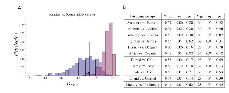
Figure 3: (A) An illustration of our bootstrap experiments. The triplet distance $D_{\mathrm{triplet}}$ between the dendrograms of the Americas and Oceania is $0.56$ (arrow). This number sits at the very low end of the distribution of distances when leaves are randomly permuted (the red shaded profile on the right), but it is well within the distribution that we obtain by randomly re-sampling from the set of languages (the blue shaded profile on the left). This gives strong evidence that each pair of subgroups share an underlying semantic network, and that the differences between them are no larger than would result from random sampling. (B) Comparing distances (the triplet $D_{\mathrm{triplet}}$ and the Robinson-Foulds $D_{\mathrm{RF}}$) among dendrograms of subgroups and two types of bootstrap experiments: permuting leaves of the dendrogram and replacing the subgroups in question with bootstrapped samples of the same sizes. $p_{1}$-values for the former bootstrap ($p_{2}$-values for the latter) are the fraction of $1000$ bootstrap samples whose distances are smaller (larger) than the observed distance. In either case $0^{\ast}$ denotes a value below $0.001$, i.e., no bootstrap sample satisfied the condition.

Another structural feature apparent in Fig. 2 is the heterogeneity of the node degrees and link weights. The numbers of polysemies involving individual meanings are uneven, possibly toward a heavy-tailed distribution (Fig. 4). This indicates concepts not only form clusters within which they are densely connected, but also exhibit different levels of being polysemous. For example, EARTH/SOIL has more than hundreds of polysemes while SALT has only a few. Having shown that some aspects of the semantic network are universal, we next ask whether the observed heterogeneous degrees of polysemy, possibly a manifestation of varying densities of near conceptual neighbors, arise as artifacts of language family structure in our sample, or if they are inherent to the concepts themselves. Simply put, is it an intrinsic property of the concept, EARTH/SOIL, to be extensively polysemous, or is it a few languages that happened to call the same concept in so many different ways.

Suppose an underlying “universal space” relative to which each language $L$ randomly draws a subset of polysemies for each concept $S$. The number of polysemies $n_{SL}$ should then be linearly proportional to both the tendency of the concept to be polysemous for being close to many other concepts, and the tendency of the language to distinguish word senses in basic vocabulary. In our network representation, a proxy for the former is the weighted degree $n_{S}$ of node $S$, and a proxy for the latter is the total weight of links $n_{L}$ in language $L$. Then the number of polysemies is expected (see Methods):

$$n_{SL}^{\mbox{\scriptsize model}}\equiv{n_{S}}\times\frac{n_{L}}{N}.$$ (1)

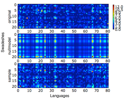
Figure 5: Plots for the data $n_{S}^{L}$, $Np^{product}_{SL}$, $n_{SL}^{sample}$ in accordance with Fig. 4S (f). The colors denote corresponding numbers of the scale. The original data in the first panel with the sample in the last panel seems to agree reasonably well.

This simple model indeed captures the gross features of the data very well (Fig. 5 in the Appendix). Nevertheless, the Kullback-Leibler divergence between the prediction $n_{SL}^{\mbox{\scriptsize model}}$ and the empirical data $n_{SL}^{\mbox{\scriptsize data}}$ identifies deviations beyond the sampling errors in three concepts—MOON, SUN and ASHES—that display nonlinear increase in the number of polysemies ($p\approx 0.01$) with the tendency of the language distinguish word senses as Fig. 6 in the Appendix shows. Accommodating saturation parameters (Table 3 in the Appendix) enables the random sampling model to reproduce the empirical data in good agreement keeping the two parameters independent, hence retain the universality over language groups.

Discussion

The similarity relations between word meanings through common polysemies exhibit a universal structure, manifested as intrinsic closeness between concepts, that transcends cultural or environmental factors. Polysemy arises when two or more concepts are fundamental enough to receive distinct vocabulary terms in some languages, yet similar enough to share a common term in others. The highly variable degree of these polysemies indicates such salient concepts are not homogeneously distributed in the conceptual space, and the intrinsic parameter that describes the overall propensity of a word to participate in polysemies can then be interpreted as a measure of the local density around such concept. Our model suggests that given the overall semantic ambiguity observed in the languages, such local density determines the degree of polysemies.

Universal structures in lexical semantics would greatly aid another subject of broad interest, namely reconstruction of human phylogeny using linguistic data Dunn2011 ; Bouckaert2012 . Much progress has been made in reconstructing the phylogenies of word forms from known cognates in various languages, thanks to the ability to measure phonetic similarity and our knowledge of the processes of sound change. However, the relationship between semantic similarity and semantic shift is still poorly understood. The standard view in historical linguistics is that any meaning can change to any other meaning Hock1986 ; Fox1995 , and that no constraint is imposed on what meanings can be compared to detect cognates Nichols1996 . It is, however, generally accepted among historical linguists that language change is gradual, and that words in transition from having one meaning to being extended to another meaning should be polysemous. If this is true, then the weights on different links reflect the probabilities that words in transition over these links will be captured in “snapshots” by language translation at any time. Such semantic shifts can be modeled as diffusion in the conceptual space, or along a universal polysemy network where our constructed networks can serve an important input to methods of inferring cognates.

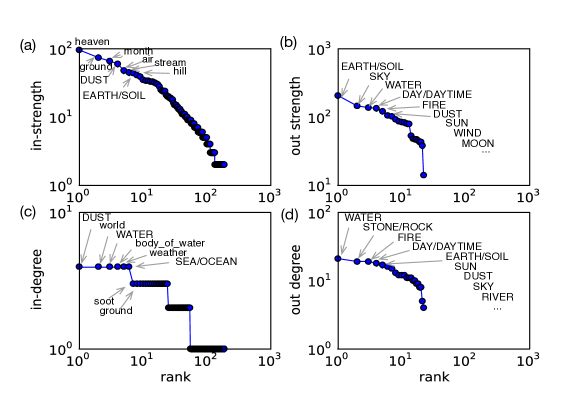
Figure 4: Rank plot of concepts in descending order of their strengths (summation of weighted links) and degrees (summation of unweighted links) shown in Fig. 2. Entries from the initial Swadesh list are distinguished with capital letters. (a) in-strengths of concepts: sum of weighted links to a node. (b) out-strengths of Swadesh entries: sum of weighted links from a Swadesh entry. (c) degree of the concepts: sum of unweighted links to a node (d) degree of Swadesh entries: sum of unweighted links to a node. A node strength in this context indicates the total number of polysemies associated with the concept in 81 languages while a node degree means the number of other concepts associated with the node regardless of the number of synonymous polysemies associated with it. heaven, for example, has the largest number of polysemies, but most of them are with SUN, so that its degree is only three.

The absence of significant cladistic correlation with the patterns of polysemy suggests a possibility to extend the constructed conceptual space by utilizing digitally archived dictionaries of the major languages of the world with some confidence that their expression of these features is not strongly biased by correlations due to language family structure. Large-corpus samples could be used to construct the semantic space in as yet unexplored domains using automated means.

Methods

Polysemy data

High-quality bilingual dictionaries between the object language and the semantic metalanguage for cross-linguistic comparison are used to identify polysemies. The 81 object languages were selected from a phylogenetically and geographically stratified sample of low-level language families or genera, listed in Tab. 1 in the Appendex Dryer1989 . Translations into the object language of each of the 22 word senses from the Swadesh basic vocabulary list were first obtained (See Appendix-.1); all translations (that is, all synonyms) were retained. Polysemies were identified by looking up the metalanguage translations (back-translation) of each object-language term. The selected Swadesh word senses, and the selected languages are listed in the Appendix.

We use modern European languages as a semantic metalanguage, i.e., bilingual dictionaries between such languages and the other languages in our sample. This could be problematic if these languages themselves display polysemies; for example, English day expresses both DAYTIME, and 24HR PERIOD. In many cases, however, the lexicographer is aware of these issues, and annotates the translation of the object language word accordingly. In the lexical domain chosen for our study, standard lexicographic practice was sufficient to overcome this problem.

Comparing semantic networks between language groups

A hierarchical spectral algorithm clusters the Swadesh word senses. Each sense $i$ is assigned to a position in $\mathbb{R}^{n}$ based on the $i$th components of the $n$ eigenvectors of the weighted adjacency matrix. Each eigenvector is weighted by the square of its eigenvalue, and clustered by a greedy agglomerative algorithm to merge the pair of clusters having the smallest squared Euclidean distance between their centers of mass, through which a binary tree or dendrogram is constructed We construct a dendrogram for each subgroup of languages according to nonlinguistic variables such as geography, topography, climate, and the presence or absence of a literary tradition (Table 2 in Appendix).

The structural distance between the dendrograms of each pair of language subgroups is measured by two standard tree metrics. The triplet distance $D_{\mathrm{triplet}}$ Dobson:75 ; Critchlow:96 is the fraction of the ${n\choose 3}$ distinct triplets of senses that are assigned a different topology in the two trees: that is, those for which the trees disagree as to which pair of senses are more closely related to each other than they are to the third. The Robinson-Foulds distance $D_{\mathrm{RF}}$ Robinson-Foulds is the number of “cuts” on which the two trees disagree, where a cut is a separation of the leaves into two sets resulting from removing an edge of the tree.

For each pair of subgroups, we perform two types of bootstrap experiments. First, we compare the distance between their dendrograms to the distribution of distances we would see under a hypothesis that the two subgroups have no shared lexical structure. Were this null hypothesis true, the distribution of distances would be unchanged under the random permutation of the senses at the leaves of each tree (For simplicity, the topology of the dendrograms are kept fixed.) Comparing the observed distance against the resulting distribution gives a $p$-value, called $p_{1}$ in Figure 3. These $p$-values are small enough to decisively reject the null hypothesis. Indeed, for most pairs of groups the Robinson-Foulds distance is smaller than that observed in any of the 1000 bootstrap trials ($p<0.001$) marked as $0^{\ast}$ in the table. This gives overwhelming evidence that the semantic network has universal aspects that apply across language subgroups: for instance, in every group we tried, SEA/OCEAN, and SALT are more related than either is to SUN.

In the second bootstrap experiment, the null hypothesis is that the nonlinguistic variables have no effect on the semantic network, and that the differences between language groups simply result from random sampling: for instance, the similarity between the Americas and Eurasia is what one would expect from any disjoint subgroups of the 81 languages of given sizes 29 and 20 respectively. To test this null hypothesis, we generate random pairs of disjoint language subgroups with the same sizes as the groups in question, and measure the distribution of their distances. The $p$-values, called $p_{2}$ in Figure 3, are not small enough to reject this null hypothesis. Thus, at least given the current data set, there is no statistical distinction between random sampling and empirical data —further supporting our thesis that it is, at least in part, universal.

Null model

The model treats all concepts as independent members of an unbiased sample that the aggregate summary statistics of the empirical data reflects the underlying structure. The simplest model perhaps then assumes no interaction between concept and languages: the number of polysemies of concept $S$ in language $L$, that is $n_{SL}^{\mbox{\scriptsize model}}$, is linearly proportional to both the tendency of the concept to be polysemous and the tendency of the language to distinguish word senses; and these tendencies are estimated from the marginal distribution of the observed data as the fraction of polysemy associated with the concept, $p_{S}^{\mbox{\scriptsize data}}=n_{S}^{\mbox{\scriptsize data}}/N$, and the fraction of polysemy in the language, $p_{S}^{\mbox{\scriptsize data}}=n_{L}^{\mbox{\scriptsize data}}/N$, respectively. The model can, therefore, be expressed as, $p_{SL}^{\mbox{\scriptsize model}}=p_{S}^{\mbox{\scriptsize data}}p_{L}^{\mbox{\scriptsize data}}$, a product of the two.

To test the model, we compare the Kullback-Leibler (KL) divergence of ensembles of the model with the observation Cover1991 . Ensembles are generated by the multinominal distribution according to the probability $p_{SL}^{\mbox{\scriptsize model}}$. The KL divergence is an appropriate measure for testing typicality of this random process because it is the leading exponential approximation (by Stirling’s formula) to the log of the multinomial distribution produced by Poisson sampling (see Appendix .4). The KL divergence of ensembles is $D\left(p_{SL}^{\mbox{\scriptsize ensemble}}\right\|\left.p_{SL}^{\mbox{\scriptsize model}}\right)\equiv\sum_{S,L}p_{SL}^{\mbox{\scriptsize ensemble}}\log\left({p_{SL}^{\mbox{\scriptsize ensemble}}}/{p_{SL}^{\mbox{\scriptsize model}}}\right)$ where $p_{SL}^{\mbox{\scriptsize ensemble}}$ is the number of polysemies that the model generates divided by $N$, and the KL divergence of the empirical observation is $D\left(p_{SL}^{\mbox{\scriptsize data}}\right\|\left.p_{SL}^{\mbox{\scriptsize model}}\right)\equiv\sum_{S,L}p_{SL}^{\mbox{\scriptsize data}}\log\left({p_{SL}^{\mbox{\scriptsize data}}}/{p_{SL}^{\mbox{\scriptsize model}}}\right)$. Note that $p_{SL}^{\mbox{\scriptsize data}}$ is ${n_{SL}}^{\mbox{\scriptsize data}}/N$ and it is a different value from an expected value of the model, ${n_{S}}^{\mbox{\scriptsize data}}{n_{L}^{\mbox{\scriptsize data}}}/N^{2}$. The $p$-value is the cumulative probability of $D\left(p_{SL}^{\mbox{\scriptsize ensemble}}\right\|\left.p_{SL}^{\mbox{\scriptsize model}}\right)$ to the right of $D\left(p_{SL}^{\mbox{\scriptsize data}}\right\|\left.p_{SL}^{\mbox{\scriptsize model}}\right)$.

Appendix

.1 Criteria for selection of meanings

Our translations use only lexical concepts as opposed to grammatical inflections or function words. For the purpose of universality and stability of meanings across cultures, we chose entries from the Swadesh 200-word list of basic vocabulary. Among these, we have selected categories that are likely to have single-word representation for meanings, and for which the referents are material entities or natural settings rather than social or conceptual abstractions. We have selected 22 words in domains concerning natural and geographic features, so that the web of polysemy will produce a connected graph whose structure we can analyze, rather than having an excess of disconnected singletons. We have omitted body parts—which by the same criteria would provide a similarly appropriate connected domain—because these have been considered previously Brown1976 ; Brown1979 ; WitkowskiBrown1978 ; BrownWitkowski1981 . The final set of 22 words are as follows:

• Celestial Phenomena and Related Time Units:
  STAR, SUN, MOON, YEAR, DAY/DAYTIME, NIGHT

• Landscape Features:
  SKY, CLOUD(S), SEA/OCEAN, LAKE, RIVER, MOUNTAIN

• Natural Substances:
  STONE/ROCK, EARTH/SOIL, SAND, ASH(ES), SALT, SMOKE, DUST, FIRE, WATER, WIND

.2 Language List

The languages included in our study are listed in Tab. 1. Notes: Oceania includes Southeast Asia; the Papuan languages do not form a single phylogenetic group in the view of most historical linguists; other families in the table vary in their degree of acceptance by historical linguists. The classification at the genus level, which is of greater importance to our analysis, is generally agreed upon.

Region	Family	Genus	Language
Africa	Khoisan	Northern	Ju|’hoan
		Central	Khoekhoegowab
		Southern	!Xóõ
	Niger-Kordofanian	NW Mande	Bambara
		Southern W. Atlantic	Kisi
		Defoid	Yorùbá
		Igboid	Igbo
		Cross River	Efik
		Bantoid	Swahili
	Nilo-Saharan	Saharan	Kanuri
		Kuliak	Ik
		Nilotic	Nandi
		Bango-Bagirmi-Kresh	Kaba Démé
	Afro-Asiatic	Berber	Tumazabt
		West Chadic	Hausa
		E Cushitic	Rendille
		Semitic	Iraqi Arabic
Eurasia	Basque	Basque	Basque
	Indo-European	Armenian	Armenian
		Indic	Hindi
		Albanian	Albanian
		Italic	Spanish
		Slavic	Russian
	Uralic	Finnic	Finnish
	Altaic	Turkic	Turkish
		Mongolian	Khalkha Mongolian
	Japanese	Japanese	Japanese
	Chukotkan	Kamchatkan	Itelmen (Kamchadal)
	Caucasian	NW Caucasian	Kabardian
		Nax	Chechen
	Katvelian	Kartvelian	Georgian
	Dravidian	Dravidian Proper	Badaga
	Sino-Tibetan	Chinese	Mandarin
		Karen	Karen (Bwe)
		Kuki-Chin-Naga	Mikir
		Burmese-Lolo	Hani
		Naxi	Naxi
Oceania	Hmong-Mien	Hmong-Mien	Hmong Njua
	Austroasiatic	Munda	Sora
		Palaung-Khmuic	Minor Mlabri
		Aslian	Semai (Sengoi)
	Daic	Kam-Tai	Thai
	Austronesian	Oceanic	Trukese
	Papuan	Middle Sepik	Kwoma
		E NG Highlands	Yagaria
		Angan	Baruya
		C and SE New Guinea	Kolari
		West Bougainville	Rotokas
		East Bougainville	Buin
	Australian	Gunwinguan	Nunggubuyu
		Maran	Mara
		Pama-Nyungan	E and C Arrernte
Americas	Eskimo-Aleut	Aleut	Aleut
	Na-Dene	Haida	Haida
		Athapaskan	Koyukon
	Algic	Algonquian	Western Abenaki
	Salishan	Interior Salish	Thompson Salish
	Wakashan	Wakashan	Nootka (Nuuchahnulth)
	Siouan	Siouan	Lakhota
	Caddoan	Caddoan	Pawnee
	Iroqoian	Iroquoian	Onondaga
	Coastal Penutian	Tsimshianic	Coast Tsimshian
		Klamath	Klamath
		Wintuan	Wintu
		Miwok	Northern Sierra Miwok
	Gulf	Muskogean	Creek
	Mayan	Mayan	Itzá Maya
	Hokan	Yanan	Yana
		Yuman	Cocopa
	Uto-Aztecan	Numic	Tümpisa Shoshone
		Hopi	Hopi
	Otomanguean	Zapotecan	Quiavini Zapotec
	Paezan	Warao	Warao
		Chimúan	Mochica/Chimu
	Quechuan	Quechua	Huallaga Quechua
	Araucanian	Araucanian	Mapudungun (Mapuche)
	Tupí-Guaraní	Tupí-Guaraní	Guaraní
	Macro-Arawakan	Harákmbut	Amarakaeri
		Maipuran	Piro
	Macro-Carib	Carib	Carib
		Peba-Yaguan	Yagua

Table 1: The languages included in our study. The classification at the genus level, which is of greater importance to our analysis, is generally agreed upon.

.3 Language groups

We performed several tests to see if the structure of the polysemy network (or whatever we’re calling it) depends in a statistically significant way on typological features, including the presence or absence of a literary tradition, geography, topography, and climate. The typological features tested, with the numbers of languages indicated for each feature shown in parentheses, are listed in Tab. 2

Variable	Subset	Size
Geography	Americas	29
	Eurasia	20
	Africa	17
	Oceania	15
Climate	Humid	38
	Cold	30
	Arid	13
Topography	Inland	45
	Coastal	36
Literary tradition	Some or long literary tradition	28
	No literary tradition	53

Table 2: Various groups of languages based on nonlinguistic variables. For each variable we measured the difference between the subsets’ semantic networks, defined as the tree distance between the dendrograms of Swadesh words generated by spectral clustering.

.4 Model for Degree of Polysemy

.4.1 Aggregation of language samples

We now consider more formally the reasons sample aggregates may not simply be presumed as summary statistics, because they entail implicit generating processes that must be tested. By demonstrating an explicit algorithm that assigns probabilities to samples of Swadesh node degrees, presenting significance measures consistent with the aggregate graph and the sampling algorithm, and showing that the languages in our dataset are typical by these measures, we justify the use and interpretation of the aggregate graph (Fig. 2 ).

We begin by introducing an error measure appropriate to independent sampling from a general mean degree distribution. We then introduce calibrated forms for this distribution that reproduce the correct sample means as functions of both Swadesh-entry and language-weight properties.

The notion of consistency with random sampling is generally scale-dependent. In particular, the existence of synonymous polysemy may cause individual languages to violate criteria of randomness, but if the particular duplicated polysemes are not correlated across languages, even small groups of languages may rapidly converge toward consistency with a random sample. Therefore, we do not present only a single acceptance/rejection criterion for our dataset, but rather show the smallest groupings for which sampling is consistent with randomness, and then demonstrate a model that reproduces the excess but uncorrelated synonymous polysemy within individual languages.

.4.2 Independent sampling from the aggregate graph

Figure  2 treats all words in all languages as independent members of an unbiased sample. To test the appropriateness of the aggregate as a summary statistic, we ask: do random samples, with link numbers equal to those in observed languages, and with link probabilities proportional to the weights in the aggregate graph, yield ensembles of graphs within which the actual languages in our data are typical?

Statistical tests

The appropriate summary statistic to test for typicality, in ensembles produced by random sampling (of links or link-ends) is the Kullback-Leibler (KL) divergence of the sample counts from the probabilities with which the samples were drawn Cover1991 . This is because the KL divergence is the leading exponential approximation (by Stirling’s formula) to the log of the multinomial distribution produced by Poisson sampling.

The appropriateness of a random-sampling model may be tested independently of how the aggregate link numbers are used to generate an underlying probability model. In this section, we will first evaluate a variety of underlying probability models under Poisson sampling, and then we will return to tests for deviations from independent Poisson samples. We first introduce notation: For a single language, the relative degree (link frequency), which is used as the normalization of a probability, is denoted as $p_{S\mid L}^{\mbox{\scriptsize data}}\equiv n_{S}^{L}/n^{L}$, and for the joint configuration of all words in all languages, the link frequency of a single entry relative to the total $N$ will be denoted $p_{SL}^{\mbox{\scriptsize data}}\equiv n_{S}^{L}/N=\left(n_{S}^{L}/n^{L}\right)\left(n^{L}/N\right)\equiv p_{S\mid L}^{\mbox{\scriptsize data}}p_{L}^{\mbox{\scriptsize data}}$.

Corresponding to any of these, we may generate samples of links to define the null model for a random process, which we denote ${\hat{n}}_{S}^{L}$, ${\hat{n}}^{L}$, etc. We will generally use samples with exactly the same number of total links $N$ as the data. The corresponding sample frequencies will be denoted by $p_{S\mid L}^{\mbox{\scriptsize sample}}\equiv{\hat{n}}_{S}^{L}/{\hat{n}}^{L}$ and $p_{SL}^{\mbox{\scriptsize sample}}\equiv{\hat{n}}_{S}^{L}/N=\left({\hat{n}}_{S}^{L}/{\hat{n}}^{L}\right)\left({\hat{n}}^{L}/N\right)\equiv p_{S\mid L}^{\mbox{\scriptsize sample}}p_{L}^{\mbox{\scriptsize sample}}$, respectively.

Finally, the calibrated model, which we define from properties of aggregated graphs, will be the prior probability from which samples are drawn to produce $p$-values for the data. We denote the model probabilities (which are used in sampling as “true” probabilities rather than sample frequencies) by $p_{S\mid L}^{\mbox{\scriptsize model}}$, $p_{SL}^{\mbox{\scriptsize model}}$, and $p_{L}^{\mbox{\scriptsize model}}$.

For $n^{L}$ links sampled independently from the distribution $p_{S\mid L}^{\mbox{\scriptsize sample}}$ for language $L$, the multinomial probability of a particular set $\left\{n_{S}^{L}\right\}$ may be written, using Stirling’s formula to leading exponential order, as

$$p\!\left(\left\{n_{S}^{L}\right\}\mid n^{L}\right)\sim e^{-n^{L}D\left(p_{S\mid L}^{\mbox{\scriptsize sample}}\right\|\left.p_{S\mid L}^{\mbox{\scriptsize model}}\right)}$$ (2)

where the Kullback-Leibler (KL) divergence Cover1991

$$D\left(p_{S\mid L}^{\mbox{\scriptsize sample}}\right\|\left.p_{S\mid L}^{\mbox{\scriptsize model}}\right)\equiv\sum_{S}p_{S\mid L}^{\mbox{\scriptsize sample}}\log\left(\frac{p_{S\mid L}^{\mbox{\scriptsize sample}}}{p_{S\mid L}^{\mbox{\scriptsize model}}}\right).$$ (3)

For later reference, note that the leading quadratic approximation to Eq. (3) is

$$n^{L}D\left(p_{S\mid L}^{\mbox{\scriptsize sample}}\right\|\left.p_{S\mid L}^{\mbox{\scriptsize model}}\right)\approx\frac{1}{2}\sum_{S}\frac{{\left({\hat{n}}_{S}^{L}-n^{L}p_{S\mid L}^{\mbox{\scriptsize model}}\right)}^{2}}{n^{L}p_{S\mid L}^{\mbox{\scriptsize model}}},$$ (4)

so that the variance of fluctuations in each word is proportional to its expected frequency.

As a null model for the joint configuration over all languages in our set, if $N$ links are drawn independently from the distribution $p_{SL}^{\mbox{\scriptsize sample}}$, the multinomial probability of a particular set $\left\{n_{S}^{L}\right\}$ is given by

$$p\!\left(\left\{n_{S}^{L}\right\}\mid N\right)\sim e^{-ND\left(p_{SL}^{\mbox{\scriptsize sample}}\right\|\left.p_{SL}^{\mbox{\scriptsize model}}\right)}$$ (5)

where

$$D\left(p_{SL}^{\mbox{\scriptsize sample}}\right\|\left.p_{SL}^{\mbox{\scriptsize model}}\right)\equiv\sum_{S,L}p_{SL}^{\mbox{\scriptsize sample}}\log\left(\frac{p_{SL}^{\mbox{\scriptsize sample}}}{p_{SL}^{\mbox{\scriptsize model}}}\right)$$

$$= D\left(p_{L}^{\mbox{\scriptsize sample}}\right\|\left.p_{L}^{\mbox{\scriptsize model}}\right)+\sum_{L}p_{L}^{\mbox{\scriptsize sample}}D\left(p_{S\mid L}^{\mbox{\scriptsize sample}}\right\|\left.p_{S\mid L}^{\mbox{\scriptsize model}}\right)\!.$$

Multinomial samples of assignments ${\hat{n}}_{S}^{L}$ to each of the $22\times 81$ $\left(\mbox{Swadesh},\mbox{Language}\right)$ pairs, with $N$ links total drawn from distribution ${p_{S}^{L}}^{\mbox{\scriptsize null}}$, will produce KL divergences uniformly distributed in the coordinate $d\Phi\equiv e^{-D_{KL}}dD_{KL}$, corresponding to the uniform increment of cumulative probability in the model distribution. We may therefore use the cumulative probability to the right of $D\left(p_{SL}^{\mbox{\scriptsize data}}\right\|\left.p_{SL}^{\mbox{\scriptsize model}}\right)$ (one-sided $p$-value), in the distribution of samples ${\hat{n}}_{S}^{L}$, as a test of consistency of our data with the model of random sampling.

In the next two subsections we will generate and test candidates for $p^{\mbox{\scriptsize model}}$ which are different functions of the mean link numbers on Swadesh concepts and the total links numbers in languages.

Product model with intrinsic property of concepts

In general we wish to consider the consistency of joint configurations with random sampling, as a function of an aggregation scale. To do this, we will rank-order languages by increasing $n^{L}$, form non-overlapping bins of 1, 3, or 9 languages, and test the resulting binned degree distributions against different mean-degree and sampling models. We denote by $\left<n^{L}\right>$ the average total link number in a bin, and by $\left<n_{S}^{L}\right>$ the average link number per Swadesh entry in the bin. The simplest model, which assumes no interaction between concept and language properties, makes the model probability $p_{SL}^{\mbox{\scriptsize model}}$ a product of its marginals. It is estimated from data without regard to binning, as

$$p_{SL}^{\mbox{\scriptsize product}}\equiv\frac{n_{S}}{N}\times\frac{n^{L}}{N}.$$ (7)

The $22\times 81$ independent mean values are thereby specified in terms of $22+81$ sample estimators.

The KL divergence of the joint configuration of links in the actual data from this model, under whichever binning is used, becomes

$$D\left(p_{SL}^{\mbox{\scriptsize data}}\right\|\left.p_{SL}^{\mbox{\scriptsize model}}\right)=D\left(\frac{\left<n_{S}^{L}\right>}{N}\left\|\frac{n_{S}}{N}\frac{\left<n^{L}\right>}{N}\right.\right)$$ (8)

As we show in Fig. 7 below, even for 9-language bins which we expect to average over a large amount of language-specific fluctuation, the product model is ruled out at the $1\%$ level.

We now show that a richer model, describing interaction between word and language properties, accepts not only the 9-language aggregate, but also the 3-language aggregate with a small adjustment of the language size to which words respond (to produce consistency with word-size and language-size marginals). Only fluctuation statistics at the level of the joint configuration of 81 individual languages remains strongly excluded by the null model of random sampling.

Product model with saturation

An inspection of the deviations of our data from the product model shows that the initial propensity of a word to participate in polysemies, as inferred in languages where that word has few links, in general overestimates the number of links (degree). Put it differently, languages seem to place limits on the weight of single polysemies, favoring distribution over distinct polysemies, but the number of potential distinct polysemies is an independent parameter from the likelihood that the available polysemies will be formed. Interpreted in terms of our supposed semantic space, the proximity of target words to a Swadesh entry may determine the likelihood that they will be polysemous with it, but the total number of proximal targets may vary independently of their absolute proximity. These limits on the number of neighbors of each concept are captured by additional 22 parameters.

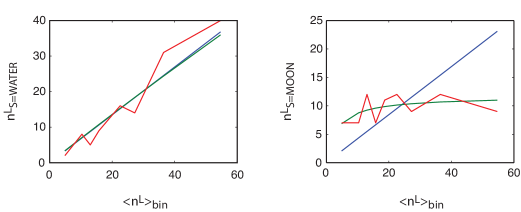
Figure 6: Plots of the saturating function (9) with the parameters given in Table 3, compared to $\left<n_{S}^{L}\right>$ (ordinate) in 9-language bins (to increase sample size), versus bin-averages $\left<n^{L}\right>$ (abscissa). Red line is drawn through data values, blue is the product model, and green is the saturation model. WATER requires no significant deviation from the product model ($B_{\rm WATER}/N\gg 20$), while MOON shows the lowest saturation value among the Swadesh entries, at $B_{\rm MOON}\approx 3.4$.

Meaning category	Saturation: $B_{S}$	Propensity ${\tilde{p}}_{S}$
STAR	$1234.2$	0.025
SUN	$25.0$	0.126
YEAR	$1234.2$	0.021
SKY	$1234.2$	0.080
SEA/OCEAN	$1234.2$	0.026
STONE/ROCK	$1234.2$	0.041
MOUNTAIN	$1085.9$	0.049
DAY/DAYTIME	$195.7$	0.087
SAND	$1234.2$	0.026
ASH(ES)	$13.8$	0.068
SALT	$1234.2$	0.007
FIRE	$1234.2$	0.065
SMOKE	$1234.2$	0.031
NIGHT	$89.3$	0.034
DUST	$246.8$	0.065
RIVER	$336.8$	0.048
WATER	$1234.2$	0.073
LAKE	$1234.2$	0.047
MOON	$1.2$	0.997
EARTH/SOIL	$1234.2$	0.116
CLOUD(S)	$53.4$	0.033
WIND	$1234.2$	0.051

Table 3: A table of fitted values of parameters $B_{S}$ and ${\tilde{p}}_{S}$ for the saturation model of Eq. (9) . The saturation value $B_{S}$ is an asymtotic number of meanings associated with the entry $S$, and the propensity ${\tilde{p}}_{S}$ is a rate at which the number of polysemies increases with $n^{L}$ at low $n_{S}^{L}$.

To accommodate such characteristic, we revise the model Eq. (7) to the following function:

$$\frac{A_{S}\left<n^{L}\right>}{B_{S}+\left<n^{L}\right>}.$$

where degree numbers $\left<n_{S}^{L}\right>$ for each Swadesh $S$ is proportional to $A_{S}$ and language size, but is bounded by $B_{S}$, the number of proximal concepts. The corresponding model probability for each language then becomes

$$p_{SL}^{\mbox{\scriptsize sat}}=\frac{(A_{S}/B_{S})(n^{L}/N)}{1+n^{L}/B_{S}} \equiv \frac{{\tilde{p}}_{S}p_{L}^{\mbox{\scriptsize data}}}{1+p_{L}^{\mbox{\scriptsize data}}N/B_{S}}.$$ (9)

As all $B_{S}/N\rightarrow\infty$ we recover the product model, with $p_{L}^{\mbox{\scriptsize data}}\equiv n^{L}/N$ and ${\tilde{p}}_{S}\rightarrow n_{S}/N$.

A first-level approximation to fit parameters $A_{S}$ and $B_{S}$ is given by minimizing the weighted mean-square error

$$E\equiv\sum_{L}\frac{1}{\left<n^{L}\right>}\sum_{S}{\left(\left<n_{S}^{L}\right>-\frac{A_{S}\left<n^{L}\right>}{B_{S}+\left<n^{L}\right>}\right)}^{2}.$$ (10)

The function (10) assigns equal penalty to squared error within each language bin $\sim\left<n^{L}\right>$, proportional to the variance expected from Poisson sampling. The fit values obtained for $A_{S}$ and $B_{S}$ do not depend sensitively on the size of bins except for the Swadesh entry MOON in the case where all 81 single-language bins are used. MOON has so few polysemies, but the MOON/month polysemy is so likely to be found, that the language Itelman, with only one link, has this polysemy. This point leads to instabilities in fitting $B_{\rm MOON}$ in single-language bins. For bins of size 3–9 the instability is removed. Representative fit parameters across this range are shown in Table 3. Examples of the saturation model for two words, plotted against the 9-language binned degree data in Fig. 6, show the range of behaviors spanned by Swadesh entries.

Figure 7: Kullback-Leibler divergence of link frequencies in our data, grouped into non-overlapping 9-language bins ordered by rank, from the product distribution (7) and the saturation model (9). Parameters $A_{S}$ and $B_{S}$ have been adjusted (as explained in the text) to match the word- and language-marginals. From 10,000 random samples ${\hat{n}}_{S}^{L}$, (green) histogram for the product model; (blue) histogram for the saturation model; (red dots) data. The product model rejects the 9-language joint binned configuration at the at $1\%$ level (dark shading), while the saturation model is typical of the same configuration at $\sim 59\%$ (light shading).

The least-squares fits to $A_{S}$ and $B_{S}$ do not directly yield a probability model consisent with the marginals for language size that, in our data, are fixed parameters rather than sample variables to be explained. They closely approximate the marginal N $\sum_{L}p_{SL}^{\mbox{\scriptsize sat}}\approx n_{S}$ (deviations $<1$ link for every $S$) but lead to mild violations $N\sum_{S}p_{SL}^{\mbox{\scriptsize sat}}\neq n^{L}$. We corrected for this by altering the saturation model to suppose that, rather than word properties’ interacting with the exact value $n^{L}$, they interact with a (word-independent but language-dependent) multiplier $\left(1+{\varphi}^{L}\right)n_{L}$, so that the model for $n_{S}^{L}$ in each language becomes becomes

$$\frac{A_{S}\left(1+{\varphi}^{L}\right)n^{L}}{B_{S}+\left(1+{\varphi}^{L}\right)n^{L}},$$

in terms of the least-squares coefficients $A_{S}$ and $B_{S}$ of Table 3. The values of ${\varphi}^{L}$ are solved with Newton’s method to produce $N\sum_{S}p_{SL}^{\mbox{\scriptsize sat}}\rightarrow n^{L}$, and we checked that they preserve $N\sum_{L}p_{SL}^{\mbox{\scriptsize sat}}\approx n_{S}$ within small fractions of a link. The resulting adjustment parameters are plotted versus $n^{L}$ for individual languages in Fig. 8. Although they were computed individually for each $L$, they form a smooth function of $n^{L}$, possibly suggesting a refinement of the product model, but also perhaps reflecting systematic interaction of small-language degree distributions with the error function (10).

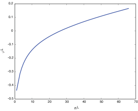
Figure 8: Plot of the correction factor ${\varphi}^{L}$ versus $n^{L}$ for individual languages in the probability model used in text, with parameters $B_{S}$ and ${\tilde{p}}_{S}$ shown in Table 3. Although ${\varphi}^{L}$ values were individually solved with Newton’s method to ensure that the probability model matched the whole-language link values, the resulting correction factors are a smooth function of $n^{L}$.

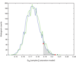
Figure 9: The same model parameters as in Fig. 7 is now marginally plausible for the joint configuration of 27 three-language bins in the data, at the $7\%$ level (light shading). For reference, this fine-grained joint configuration rejects the null model of independent sampling from the product model at $p-value\approx{10}^{-3}$ (dark shading in the extreme tail). 4000 samples were used to generate this test distribution. The blue histogram is for the saturation model, the green histogram for the product model, and the red dots are generated data.

With the resulting joint distribution $p_{SL}^{\mbox{\scriptsize sat}}$, tests of the joint degree counts in our dataset for consistency with multinomial sampling in 9 nine-language bins are shown in Fig. 7, and results of tests using 27 three-language bins are shown in Fig. 9. Binning nine languages clearly averages over enough language-specific variation to make the data strongly typical of a random sample ($P\sim 59\%$), while the product model (which also preserves marginals) is excluded at the $1\%$ level. The marginal acceptance of the data even for the joint configuration of three-language bins ($P\sim 7\%$) suggests that language size $n^{L}$ is an excellent explanatory variable and that residual language variations cancel to good approximation even in small aggregations.

.4.3 Single instances as to aggregate representation

The preceding subsection showed intermediate scales of aggregation of our language data are sufficiently random that they can be used to refine probability models for mean degree as a function of parameters in the globally-aggregated graph. The saturation model, with data-consistent marginals and multinomial sampling, is weakly plausible by bins of as few as three languages. Down to this scale, we have therefore not been able to show a requirement for deviations from the independent sampling of links entailed by the use of the aggregate graph as a summary statistic. However, we were unable to find a further refinement of the mean distribution that would reproduce the properties of single language samples. In this section we characterize the nature of their deviation from independent samples of the saturation model, show that it may be reproduced by models of non-independent (clumpy) link sampling, and suggest that these reflect excess synonymous polysemy.

Power tests and uneven distribution of single-language $p$-values

To evaluate the contribution of individual languages versus language aggregates to the acceptance or rejection of random-sampling models, we computed $p$-values for individual languages or language bins, using the KL-divergence (3). A plot of the single-language $p$-values for both the null (product) model and the saturation model is shown in Fig. 10. Histograms for both single languages (from the values in Fig. 10) and aggregate samples formed by binning consecutive groups of three languages are shown in Fig. 11.

For samples from a random model, $p$-values would be uniformly distributed in the unit interval, and histogram counts would have a multinomial distribution with single-bin fluctuations depending on the total sample size and bin width. Therefore, Fig. 11 provides a power test of our summary statistics. The variance of the multinomial may be estimated from the large-$p$-value body where the distribution is roughly uniform, and the excess of counts in the small-$p$-value tail, more than one standard deviation above the mean, provides an estimate of the number of languages that can be confidently said to violate the random-sampling model.

From the upper panel of Fig. 11, with a total sample of 81 languages, we can estimate a number of $\sim 0.05\times 81\approx 4-5$ excess languages at the lowest $p$-values of 0.05 and 0.1, with an additional 2–3 languages rejected by the product model in the range $p$-value $\sim 0.2$. Comparable plots in Fig. 11 (lower panel) for the 27 three-language aggregate distributions are marginally consistent with random sampling for the saturation model, as expected from Fig. 9 above. We will show in the next section that a more systematic trend in language fluctuations with size provides evidence that the cause for these rejections is excess variance due to repeated attachment of links to a subset of nodes.

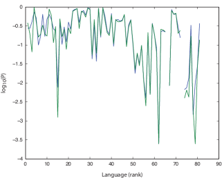
Figure 10: $\log_{10}\!\left(p\rm{-value}\right)$ by KL divergence, relative to 4000 random samples per language, plotted versus language rank in order of increasing $n^{L}$. Product model (green) shows equal or lower $p$-values for almost all languages than the saturation model (blue). Three languages – Basque, Haida, and Yorùbá – had value $p=0$ consistently across samples in both models, and are removed from subsequent regression estimates. A trend toward decreasing $p$ is seen with increase in $n^{L}$.

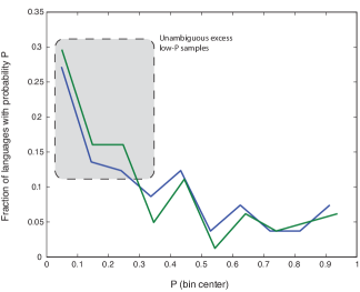
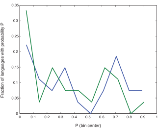
Figure 11: (Upper panel) Normalized histogram of $p$-values from the 81 languages plotted in Fig. 10. The saturation model (blue) produces a fraction $\sim 0.05\times 81\approx 4-5$ languages in the lowest $p$-values $\left\{0.05,0.1\right\}$ above the roughly-uniform background for the rest of the interval (shaded area with dashed boundary). A further excess of 2–3 languages with $p$-values in the range $\left[0,0.2\right]$ for the product model (green) reflects the part of the mismatch corrected through mean values in the saturation model. (Lower panel) Corresponding histogram of $p$-values for 27 three-language aggregate degree distributions. Saturation model (blue) is now marginally consistent with a uniform distribution, while the product model (green) still shows slight excess of low-$p$ bins. Coarse histogram bins have been used in both panels to compensate for small sample numbers in the lower panel, while producing comparable histograms.

Excess fluctuations in degree of polysemy

If we define the size-weighted relative variance of a language analogously to the error term in Eq. (10), as

$${\left({\sigma}^{2}\right)}^{L}\equiv\frac{1}{n^{L}}\sum_{S}{\left(n_{S}^{L}-n^{L}p_{S\mid L}^{\mbox{\scriptsize model}}\right)}^{2},$$ (11)

Fig. 12 shows that $-\log_{10}\!\left(p{\rm-value}\right)$ has high rank correlation with ${\left({\sigma}^{2}\right)}^{L}$ and a roughly linear regression over most of the range. Two languages (Itelmen and Hindi), which appear as large outliers relative to the product model, are within the main dispersion in the saturation model, showing that their discrepency is corrected in the mean link number. We may therefore understand a large fraction of the improbability of languages as resulting from excess fluctuations of their degree numbers relative to the expectation from Poisson sampling.

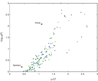
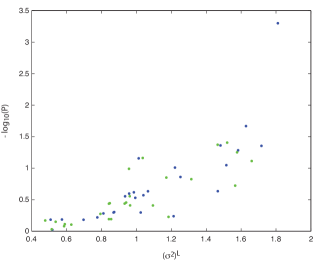
Figure 12: (Upper panel:) $-\log_{10}\!\left(P\right)$ plotted versus relative variance ${\left({\sigma}^{2}\right)}^{L}$ from Eq. (11) for the 78 languages with non-zero $p$-values from Fig. 10. (blue) saturation model; (green) product model. Two languages (circled) which appear as outliers with anomalously small relative variance in the product model – Itelman and Hindi – disappear into the central tendency with the saturation model. (Lower panel:) an equivalent plot for 26 three-language bins. Notably, the apparent separation of individual large-$n^{L}$ langauges into two groups has vanished under binning, and a unimodal and smooth dependence of $-\log_{10}\!\left(P\right)$ on ${\left({\sigma}^{2}\right)}^{L}$ is seen.

Fig. 13 then shows the relative variance from the saturation model, plotted versus total average link number for both individual languages and three-language bins. The binned languages show no significant regression of relative variance away from the value unity for Poisson sampling, whereas single languages show a systematic trend toward larger variance in larger languages, a pattern that we will show is consistent with “clumpy” sampling of a subset of nodes. The disappearance of this clumping in binned distributions shows that the clumps are uncorrelated among languages at similar $n^{L}$.

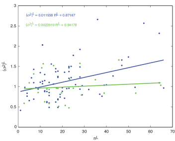
Figure 13: Relative variance from the saturation model versus total link number $n^{L}$ for 78 languages excluding Basque, Haida, and Yorùbá. Least-squares regression are shown for three-language bins (green) and individual languages (blue), with regression coefficients inset. Three-language bins are consistent with Poisson sampling at all $n^{L}$, whereas single languages show systematic increase of relative variance with increasing $n^{L}$.

Correlated link assignments

We may retain the mean degree distributions, while introducing a systematic trend of relative variance with $n^{L}$, by modifying our sampling model away from strict Poisson sampling to introduce “clumps” of links. To remain within the use of minimal models, we modify the sampling procedure by a single parameter which is independent of word $S$, language-size $n^{L}$, or particular language $L$.

We introduce the sampling model as a function of two parameters, and show that one function of these is constrained by the regression of excess variance. (The other may take any interior value, so we have an equivalence class of models.) In each language, select a number $\mathcal{B}$ of Swadesh entries randomly. Let the Swadesh indices be denoted ${\left\{S_{\beta}\right\}}_{\beta\in 1,\ldots\mathcal{B}}$. We will take some fraction of the total links in that language, and assign them only to the Swadeshes whose indices are in this privileged set. Introduce a parameter $q$ that will determine that fraction.

We require correlated link assignments be consistent with the mean determined by our model fit, since binning of data has shown no systematic effect on mean parameters. Therefore, for the random choice ${\left\{S_{\beta}\right\}}_{\beta\in 1,\ldots\mathcal{B}}$, introduce the normalized density on the privileged links

$${\pi}_{S\mid L}\equiv\frac{p_{S\mid L}^{\mbox{\scriptsize model}}}{\sum_{\beta=1}^{\mathcal{B}}p_{S_{\beta}\mid L}^{\mbox{\scriptsize model}}}$$ (12)

if $S\in{\left\{S_{\beta}\right\}}_{\beta\in 1,\ldots\mathcal{B}}$ and ${\pi}_{S\mid L}=0$ otherwise. Denote the aggregated weight of the links in the priviledged set by

$$W\equiv\sum_{\beta=1}^{\mathcal{B}}p_{S_{\beta}\mid L}.$$ (13)

Then introduce a modified probability distribution based on the randomly selected links, in the form

$${\tilde{p}}_{S\mid L}\equiv\left(1-qW\right)p_{S\mid L}+qW{\pi}_{S\mid L}.$$ (14)

Multinomial sampling of $n^{L}$ links from the distribution ${\tilde{p}}_{S\mid L}$ will produce a size-dependent variance of the kind we see in the data. The expectated degrees given any particular set ${\left\{S_{\beta}\right\}}$ will not agree with the means in the aggregate graph, but the ensemble mean over random samples of languages will equal $p_{S\mid L}$, and binned groups of languages will converge toward it according to the central-limit theorem.

The proof that the relative variance increases linearly in $n^{L}$ comes from the expansion of the expectation of Eq. (11) for random samples, denoted

$$\left<{\left({\hat{\sigma}}^{2}\right)}^{L}\right>\equiv\left<\frac{1}{n^{L}}\sum_{S}{\left({\hat{n}}_{S}^{L}-n^{L}p_{S\mid L}^{\mbox{\scriptsize model}}\right)}^{2}\right>$$ (15)

$$= \left<\frac{1}{n^{L}}\sum_{S}{\left[\left({\hat{n}}_{S}^{L}-n^{L}{\tilde{p}}_{S\mid L}\right)+n^{L}\left({\tilde{p}}_{S\mid L}-p_{S\mid L}^{\mbox{\scriptsize model}}\right)\right]}^{2}\right>$$

$$= \left<\frac{1}{n^{L}}\sum_{S}{\left({\hat{n}}_{S}^{L}-n^{L}{\tilde{p}}_{S\mid L}\right)}^{2}\right>+$$

$$\qquad n^{L}\left<\sum_{S}{\left({\tilde{p}}_{S\mid L}-p_{S\mid L}^{\mbox{\scriptsize model}}\right)}^{2}\right>.$$

The first expectation over ${\hat{n}}_{S}^{L}$ is constant (of order unity) for Poisson samples, and the second expectation (over the sets ${\left\{S_{\beta}\right\}}$ that generate ${\tilde{p}}_{S\mid L}$) does not depend on $n^{L}$ except in the prefactor. Cross-terms vanish because link samples are not correlated with samples of ${\left\{S_{\beta}\right\}}$. Both terms in the third line of Eq. (15) scale under binning as ${\left(\mbox{bin-size}\right)}^{0}$. The first term is invariant due to Poisson sampling, while in the second term, the central-limit theorem reduction of the variance in samples over ${\tilde{p}}_{S\mid L}$ cancels growth in the prefactor $n^{L}$ due to aggregation.

Because the linear term in Eq. (15) does not systematically change under binning, we interpret the vanishing of the regression for three-language bins in Fig. 13 as a consequence of fitting of the mean value to binned data as sample estimators. Therefore, we require to choose parameters $\mathcal{B}$ and $q$ so that regression coefficients in the data are typical in the model of clumpy sampling, while regressions including zero have non-vanishing weight in models of three-bin aggregations.

Fig. 14 compares the range of regression coefficients obtained for random samples of languages with the values $\left\{n^{L}\right\}$ in our data, from either the original saturation model $p_{S\mid L}^{\mbox{\scriptsize sat}}$, or the clumpy model ${\tilde{p}}_{S\mid L}$ randomly re-sampled for each language in the joint configuration. Parameters used were ($\mathcal{B}=7$, $q=0.975$). With these parameters, $\sim 1/3$ of links were assigned in excess to $\sim 1/3$ of words, with the remaining $2/3$ of links assigned according to the mean distribution.

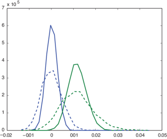
Figure 14: Histograms of regression coefficients for language link samples $\left\{{\hat{n}}_{S}^{L}\right\}$ either generated by Poisson sampling from the saturation model $p_{S\mid L}^{\mbox{\scriptsize model}}$ fitted to the data (blue), or drawn from clumped probabilities ${\tilde{p}}_{S\mid L}$ defined in Eq. (14), with the set of privileged words $\left\{S_{\beta}\right\}$ independently drawn for each language (green). Solid lines refer to joint configurations of 78 individual languages with the $n^{L}$ values in Fig. 13. Dashed lines are 26 non-overlapping three-language bins.

The important features of the graph are: 1) Binning does not change the mean regression coefficient, verifying that Eq. (15) scales homogeneously as ${\left(\mbox{bin-size}\right)}^{0}$. However, the variance for binned data increases due to reduced number of sample points; 2) the observed regression slope 0.012 seen in the data is far out of the support of multinomial sampling from $p_{S\mid L}^{\mbox{\scriptsize sat}}$, whereas with these parameters, it becomes typical under $\left\{{\tilde{p}}_{S\mid L}\right\}$ while still leaving significant probability for the three-language binned regression around zero (even without ex-post fitting).

References

- (1) Whorf BL, Language, Thought and Reality: Selected Writing. (MIT Press, Cambridge, 1956).
- (2) Fodor JA, The language of thought. (Harvard Univ., New York, 1975).
- (3) Wierzbicka, A., Semantics: primes and universals. (Oxford University Press. 1996)
- (4) Lucy JA, Grammatical categories and cognition: a case study of the linguistic relativity hypothesis. (Cambridge University Press, 1992).
- (5) Levinson SC, Space in language and cognition: explorations in cognitive diversity. (Cambridge University Press, 2003)
- (6) Choi S, Bowerman M (1991) Learning to express motion events in English and Korean: The influence of language-specific lexicalization patterns. Cognition 41, 83-121.
- (7) Majid A, Boster JS, Bowerman M (2008) Cognition 109, 235-250.
- (8) Croft W (2010) Relativity, linguistic variation and language universals. CogniTextes 4, 303.
- (9) Evans N, Levinson SC (2009) The myth of language universals: language diversity and its importance for cognitive science. Behav. Brain Sci. 21 429-492.
- (10) Comrie B Language universals and linguistic typology, 2nd ed. (University of Chicago Press., 1989).
- (11) Croft W, Typology and universals, 2nd ed. (Cambridge University Press. 2003).
- (12) Henrich J, Heine SJ, Norenzayan A (2010) The weirdest people in the world? Behav. Brain Sci. 33 1-75 (2010).
- (13) Shopen T (ed.), Language typology and syntactic description, 2nd ed. (3 volumes) (Cambridge University Press, Cambridge, 2007).
- (14) Croft W, Cruse DA, Cognitive linguistics. (Cambridge University Press. 2004).
- (15) Koptjevskaja-Tamm M, Vanhove M (2012) New directions in lexical typology. Linguistics 50, 3.
- (16) Brown CH (1976) General principles of human anatomical partonomy and speculations on the growth of partonomic nomenclature. Am. Ethnol. 3, 400-424 (1976).
- (17) Witkowski SR, Brown CH (1978) Lexical universals, Ann. Rev. of Anthropol. 7 427-51.
- (18) Brown CH (1983) Where do cardinal direction terms come from? Anthropological Linguistics 25, 121-161.
- (19) Viberg Å (1983) The verbs of perception: a typological study. Linguistics 21, 123-162.
- (20) Evans N, Multiple semiotic systems, hyperpolysemy, and the reconstruction of semantic change in Australian languages. in Diachrony within synchrony: language history and cognition (Peter Lang. Frankfurt, 1992).
- (21) Derrig S (1978) Metaphor in the color lexicon. Chicago Linguistic Society, the Parasession on the Lexicon 85-96.
- (22) Swadesh M (1952) Lexico-statistical dating of prehistoric ethnic contacts. P. Am. Philos. Soc. 96, 452-463.
- (23) Vygotsky L, Thought and Language. (MIT Press, Cambridge, MA, 2002).
- (24) Critchlow DE, Pearl DK, Qian CL (1996) The triples distance for rooted bifurcating phylogenetic trees. Syst. Biol. 45, 323–334.
- (25) Dobson AJ, Comparing the Shapes of Trees, Combinatorial mathematics III, (Springer-Verlag, New York 1975).
- (26) Robinson DF, Foulds LR (1981) Comparison of phylogenetic trees. Math. Biosci. 53, 131–147.
- (27) Dunn M, et al. (2011) Evolved structure of language shows lineage-specific trends in word-order universals. Nature 473, 79-82.
- (28) Bouckaert R, et al. (2012) Mapping the origins and expansion of the Indo-European language family. Science 337, 957.
- (29) Fox A, Linguistic reconstruction: an introduction to theory and method. (Oxford University Press. 1995).
- (30) Hock HH Principles of historical linguistics. (Mouton de Gruyter, Berlin, 1986).
- (31) Nichols J, The comparative method as heuristic. in The comparative method reviewed: regularity and irregularity in language change (Oxford University Press, 1996).
- (32) Dryer MS (1989) large linguistic areas and language sampling. Studies in Language 13, 257-292.
- (33) Cover TM, and Thomas JA, Elements of Information Theory, (Wiley, New York, 1991).
- (34) Brown CH, A theory of lexical change (with examples from folk biology, human anatomical partonomy and other domains). Anthropol. Linguist. 21, 257-276 (1979).
- (35) Brown CH & Witkowski SR, Figurative language in a universalist perspective. Am. Ethnol. 8 596-615 (1981).