Dynamo Effects Near Transition from Solar to Anti-Solar Differential Rotation

Abstract

Numerical MHD simulations play increasingly important role for understanding mechanisms of stellar magnetism. We present simulations of convection and dynamos in density-stratified rotating spherical fluid shells. We employ a new 3D simulation code for the solution of a physically consistent anelastic model of the process with a minimum number of parameters. The reported dynamo simulations extend into a “buoyancy-dominated” regime where the buoyancy forcing is dominant while the Coriolis force is no longer balanced by pressure gradients and strong anti-solar differential rotation develops as a result. We find that the self-generated magnetic fields, despite being relatively weak, are able to reverse the direction of differential rotation from anti-solar to solar-like. We also find that convection flows in this regime are significantly stronger in the polar regions than in the equatorial region, leading to non-oscillatory dipole-dominated dynamo solutions, and to concentration of magnetic field in the polar regions. We observe that convection has different morphology in the inner and at the outer part of the convection zone simultaneously such that organized geostrophic convection columns are hidden below a near-surface layer of well-mixed highly-chaotic convection. While we focus the attention on the buoyancy-dominated regime, we also demonstrate that conical differential rotation profiles and persistent regular dynamo oscillations can be obtained in the parameter space of the rotation-dominated regime even within this minimal model.

1 Introduction

Recent progress in observational and computational capabilities have led to substantial advances in our understanding of the origins of stellar and planetary magnetism and variability. The key role is played by dynamo processes driven by convection in the presence of rotation. This process is particularly complex in the case of turbulent convection in stellar and planetary envelopes. The interaction of convection, magnetic field and rotation results in variations of the rotation rate with depth and latitude, called differential rotation, and also in large-scale meridional flows. The differential rotation is a crucial part of dynamo mechanisms. It has been measured quite accurately for the solar surface by tracking motion of various features and also through analysis of the Doppler shift of spectral lines. Moreover, helioseismology data from the SOHO and SDO space missions and from the ground-based network GONG have provided measurements of the internal rotation (e.g. Schou et al., 1998) and of the meridional circulation of the Sun (Zhao et al., 2013).

Recently, high-precision spectroscopic and photometric observations have enabled measurements of the differential rotation on other stars. The most prominent feature of the solar differential rotation is that the equatorial zone rotates faster than higher latitude regions. For other stars, this type of differential rotation is called solar-like rotation. When the equator rotates slower than the polar regions then such rotational profile is called anti-solar. Anti-solar differential rotation has been observed by Doppler imaging techniques on several K-giant stars (Strassmeier et al., 2003; Kovári et al., 2015). Recent analysis of the high-precision light curves from the Kepler mission for a sample of 50 G-type stars by Reinhold & Arlt (2015) found 21–34 stars with the solar-like differential rotation and 5–10 stars with the anti-solar rotation. The latter work awaits confirmation from independent studies.

One of the first theories of non-linear convection in rotating shells developed in the Boussinesq approximation by Busse (1970), also (Busse, 1973), demonstrated that the dynamical effects of rotation on convection are a primary mechanism of stellar differential rotation. This theory revealed that the basic properties of differential rotation primarily depend on the supercritical value of the Rayleigh number which measures the strength of the buoyancy forces and determines the magnitude of convection motions. For a relatively small supercritical Rayleigh numbers convection develops mostly in the equatorial region in the form of convective rolls (also known as ”banana cells”) oriented along the rotation axis. Angular momentum transport by these cells causes solar-like differential rotation. This regime of weakly supercritical Rayleigh numbers corresponds to small Rossby numbers defined as the ratio of the rms convective velocity to the mean rotational velocity. This regime is called rotationally-dominated. Early numerical simulations in the Boussinesq approximation by Gilman (1976) confirmed these results, and also found that at high supercritical Rayleigh numbers when convection develops at all latitudes differential rotation may become anti-solar. This regime is characterized by large (typically greater than 1) Rossby numbers and is called buoyancy-dominated.. While the rotationally-dominated regime is likely to occur in the deep convection zone where convective velocities are small, Gilman & Foukal (1979) noticed that on the Sun a typical supergranulation turn-over time is much shorter than the rotation period, and thus the convection is in the bouyancy-dominated regime. This suggests that on the Sun a combination of the two regimes takes place, resulting in a complicated differential rotation profile.

Indeed, the differential rotation profile of the Sun determined by helioseismology (e.g. Schou et al., 1998) turned out to be quite different from the theoretical predictions. It is characterised by nearly radial orientation of angular velocity at midlatitudes (the so-called “conical profile”). The angular velocity also decreases monotonically from the equator to the poles by about 30%. In addition, helioseismology inferences reveal two narrow rotational shear layers at the boundaries of the convection zone: the so-called tachocline at the bottom and a near-surface shear layer at the top.

Substantial efforts have been made to reproduce the observed solar rotation in three-dimensional numerical simulations. These efforts are reviewed by Miesch (2005) and more recently by Brun et al. (2014). Historically, simulations have been successful in reproducing the decrease of angular velocity from equator to poles. However, it is a major discrepancy that most simulations tended to feature angular velocity contours parallel to the rotation axis (the so-called “cylindrical profiles”), rather than conical profiles. The profile of the differential rotation is governed by the zonal component of the vorticity equation and its analysis suggests that cylindrical profiles may be avoided if (a) baroclinic forcing with non-vanishing latitudinal entropy gradient exists, or if (b) sufficiently strong Reynolds stresses or (c) Lorentz forces develop (e.g. Miesch, 2005; Miesch et al., 2006). Pursuing alternative (a), Miesch et al. (2006) imposed a latitudinal gradient of entropy as a bottom boundary condition in global convection simulations. They were so successful in finding conical differential rotation profiles that many groups have subsequently adopted this model as standard (e.g. Browning et al., 2006; Nelson et al., 2013; Fan & Fang, 2014). While there is physical justification for a non-vanishing latitudinal entropy gradient, this model assumption must be regarded with caution as the imposed latitudinal variations in entropy have not been generated self-consistently by the convective motions in the simulations. Large amplitude Reynolds stresses required to realize alternative (b) can be achieved by driving convection more strongly. Because most early studies argued that the solar magnetic field cannot exert a substantial control over differential rotation, alternative (b) has been explored most often. A recent work in this direction is the attempt of Guerrero et al. (2013b) to find a regime close to the real solar rotation by varying the gradient of the background specific entropy and the frame rotation rate in a numerical anelastic model. These variations correspond to an increasing effective Rayleigh number and thus to a more strongly driven convection. However, the simulations did not find an intermediate regime with a “conical” profile. Instead they surprisingly showed that the transition between the solar and anti-solar rotational profiles is rather sharp. Most recently similar results have been reported by Gastine et al. (2013, 2014); Käpylä et al. (2014); Mabuchi et al. (2015), and Karak et al. (2015).

Alternative (c), namely that dynamo effects are crucial in shaping the profile of differential rotation, is much less explored. A significant number of dynamo simulations have been published previously, but most of them aimed to reproduce and explain solar magnetic features and activity cycles, (e.g. Browning et al., 2006; Ghizaru et al., 2010; Nelson et al., 2013). Only recently few studies, of which we mention (Fan & Fang, 2014; Mabuchi et al., 2015), have appeared that aim to investigate whether the solar magnetic field plays an active role in shaping the solar differential rotation profile. These studies report evidence in support of this hypothesis. This is hardly surprising as it is well-established that the main effect of self-sustained magnetic field on convection is to suppress differential rotation (e.g. Grote & Busse, 2001; Busse et al., 2003; Simitev & Busse, 2005). This finding is confirmed by Aubert (2005) and Yadav et al. (2013) who also provide scaling laws for this effect. However, the effects of dynamo action on convection in the buoyancy-dominated regime are less well explored. Studies include the afore mentioned papers by (Fan & Fang, 2014; Karak et al., 2015; Mabuchi et al., 2015) who report a number of similar results but their models are rather different from each other and in all cases also include factors that contribute to baroclinic forcing such that hypothesis (c) is not addressed in isolation.

In this context our paper has several goals. We wish to study the effects of self-generated magnetic fields on the convective flows of a density-stratified fluid in rotating spherical shell using a minimal self-consistent model. We wish to focus the attention on dynamos near the transition to buoyancy-dominated convection but we also report selected results in the rotation-dominated regime. To this end, we employ the so-called Lantz-Braginsky anelastic approximation (Braginsky & Roberts, 1995; Lantz & Fan, 1999; Jones et al., 2011). It has the advantages that the dynamics of the system depends on a minimal number of non-dimensional parameters while ad-hoc parametrizations of physical effects that may be used to better “fit” observations are excluded. We present a newly implemented numerical simulation code for the solution of the Lantz-Braginsky anelastic equations, as well as code validation results based on published benchmark solutions against four other independently-developed codes (Jones et al., 2011). Since the dynamo processes operating in the Sun and stars are still subjects to controversies with various competing proposals, we believe that it is important that our results are readily reproducible by other groups.

In Section 2 we introduce the mathematical model based on the anelastic approximation, and discuss the numerical method and diagnostic output. In Section 2.5 we present the benchmark validation results. In Section 3 we discuss the properties of dynamos in the buoyancy-dominated regime of convection. In Section 4 we demonstrate that conical differential rotation profiles and persistent regular dynamo oscillations can be obtained in the rotation-dominated regime. In Section 5, we present a summary of our main results and compare them to related recent studies. We also outline topics for future research.

2 Mathematical model and numerical method

We consider an electrically conducting, perfect gas confined to a spherical shell. The shell rotates with a fixed angular velocity $\Omega\hat{\mbox{\boldmath$k$}}$ about the vertical axis and an entropy contrast $\Delta S$ is imposed between its inner and outer surfaces.

2.1 Anelastic governing equations

Assuming a gravity field proportional to $1/r^{2}$, a hydrostatic polytropic reference state exists of the form

$$\bar{\rho}=\rho_{c}\zeta^{n},\quad\bar{T}=T_{c}\zeta,\quad\bar{P}=P_{c}\zeta^{n+1},\quad\zeta=c_{0}+c_{1}d/r,$$ (1)

with parameters $c_{0}=(2\zeta_{o}-\eta-1)/(1-\eta)$, $c_{1}=(1+\eta)(1-\zeta_{o})/(1-\eta)^{2}$, $\zeta_{o}=(\eta+1)/(\eta\exp(N_{\rho}/n)+1)$. The parameters $\rho_{c}$, $P_{c}$ and $T_{c}$ are reference values of density, pressure and temperature at the middle of the shell. The gas polytropic index $n$, the density scale height number, $N_{\rho}$, and the radius ratio, $\eta$, are defined below. Convection and magnetic field generation are described by the equations of continuity, momentum, energy and magnetic flux. In the anelastic approximation (Gough, 1969; Braginsky & Roberts, 1995; Lantz & Fan, 1999; Jones et al., 2011) these equations take the form

$$\nabla\cdot\bar{\rho}\mbox{\boldmath$u$}=0,\quad\nabla\cdot\mbox{\boldmath$B$}=0,$$ (2a)

$$\partial_{t}\mbox{\boldmath$u$}+(\nabla\times\mbox{\boldmath$u$})\times\mbox{\boldmath$u$}=-\nabla\Pi-\tau(\hat{\mbox{\boldmath$k$}}\times\mbox{\boldmath$u$})+\frac{\mathrm{R}}{\mathrm{Pr}}\frac{S}{r^{2}}\hat{\mbox{\boldmath$r$}}+\mbox{\boldmath$F$}_{\nu}+\frac{1}{\bar{\rho}}(\nabla\times\mbox{\boldmath$B$})\times\mbox{\boldmath$B$},$$ (2b)

$$\partial_{t}S+\mbox{\boldmath$u$}\cdot\nabla S=\frac{1}{\mathrm{Pr}\bar{\rho}\bar{T}}\nabla\cdot\bar{\kappa}\bar{\rho}\bar{T}\nabla S+\frac{c_{1}\mathrm{Pr}}{\mathrm{R}\bar{T}}\left(Q_{\nu}+\frac{1}{\mathrm{Pm}\bar{\rho}}Q_{j}\right),$$ (2c)

$$\partial_{t}\mbox{\boldmath$B$}=\nabla\times(\mbox{\boldmath$u$}\times\mbox{\boldmath$B$})+\mathrm{Pm}^{-1}\nabla^{2}\mbox{\boldmath$B$},$$ (2d)

where $u$ is the velocity, $B$ is the magnetic flux density, $S$ is the entropy and $\nabla\Pi$ includes all terms that can be written as gradients. The viscous force ($\mbox{\boldmath$F$}_{\nu}$), and the viscous ($Q_{\nu}$) and Joule ($Q_{j}$) heating are defined in terms of the deviatoric stress tensor ($\hat{S}_{ij}$)

$$\hat{S}_{ij}=2\bar{\nu}\bar{\rho}(e_{ij}-e_{kk}\delta_{ij}/3),\quad e_{ij}=(\partial_{i}u_{j}+\partial_{j}u_{i})/2,$$

$$\mbox{\boldmath$F$}_{\nu}=\frac{\rho_{c}}{\bar{\rho}}\nabla\cdot\mbox{\boldmath$\hat{S}$},\quad Q_{\nu}=\mbox{\boldmath$\hat{S}$}:\mbox{\boldmath$e$},\quad Q_{j}=(\nabla\times\mbox{\boldmath$B$})^{2},$$ (3)

where the double-dots symbol (:) denotes the Frobenius inner product. We assume that the viscosity $\nu$ and the entropy diffusivity $\kappa$ are constant throughout the shell. The governing equations are parametrized using the thickness of the shell $d=r_{o}-r_{i}$ as a unit of length, $d^{2}/\nu$ as a unit of time, $\Delta S$ as a unit of entropy, $\nu\sqrt{\mu_{0}\rho_{c}}/d$ as a unit of magnetic induction, $\rho_{c}$ as a unit of density and $T_{c}$ as a unit of temperature. Here, $r_{i}$ and $r_{o}$ are the inner and the outer radius, $\lambda$ and $\mu_{0}$ are the magnetic diffusivity and permeability, respectively. The system is then characterized by eight non-dimensional parameters: the radius ratio $\eta=r_{i}/r_{o}$, the polytropic index $n$, the density scale number $N_{\rho}=\ln\big{(}\bar{\rho}(r_{i})/\bar{\rho}(r_{o})\big{)}$, the Rayleigh number $\mathrm{R}={c_{1}T_{c}d^{2}\Delta S}/{(\nu\kappa)}$, the thermal Prandtl number $\mathrm{Pr}={\nu}/{\kappa}$, the magnetic Prandtl number $\mathrm{Pm}={\nu}/{\lambda}$, and the Coriolis number $\tau={2\Omega d^{2}}/{\nu}$.

Since the mass flux $\mbox{\boldmath$v$}\equiv\bar{\rho}\mbox{\boldmath$u$}$, and the magnetic flux density $B$ are solenoidal vector fields, we employ a decomposition in poloidal and toroidal components,

$$\bar{\rho}\mbox{\boldmath$u$}=\nabla\times(\nabla\times\hat{\mbox{\boldmath$r$}}rv)+\nabla\times\hat{\mbox{\boldmath$r$}}r^{2}w,$$ (4a)

$$\mbox{\boldmath$B$}=\nabla\times(\nabla\times\hat{\mbox{\boldmath$r$}}h)+\nabla\times\hat{\mbox{\boldmath$r$}}g,$$ (4b)

where $\hat{\mbox{\boldmath$r$}}$ is the radial unit vector, $r$ is the length of the position vector $r$, $v$, $w$, $h$ and $g$ are the poloidal and toroidal scalars of the momentum and magnetic field, respectively. Equations (2a) are then satisfied automatically. Scalar equations for $v$ and $w$ are obtained, and effective pressure gradients are eliminated by taking $\hat{\mbox{\boldmath$r$}}\cdot\nabla\times\nabla\times$ and $\hat{\mbox{\boldmath$r$}}\cdot\nabla\times$ of Equation (2b). Similarly, equations for $h$ and $g$ are obtained by taking $\hat{\mbox{\boldmath$r$}}\cdot\nabla\times$ and $\hat{\mbox{\boldmath$r$}}\cdot$ of Equation (2d). Spectral projections of the resulting poloidal-toroidal equations are presented in Appendix A, see also Section 2.3.

2.2 Boundary conditions

Equations (2) must be supplemented by boundary conditions. For the simulation results presented in this work the following boundary conditions are used. The inner and the outer surfaces of the shell are assumed as stress-free, impenetrable boundaries for the flow

$$v=0,\quad\partial_{r}^{2}v-\frac{\bar{\rho}^{\prime}}{\bar{\rho}r}\partial_{r}{}(rv)=0,\quad\partial_{r}w-\frac{\bar{\rho}^{\prime}}{\bar{\rho}}w=0,\quad\text{at}\quad r=r_{i},r_{o}.$$ (5)

In several cases discussed in Section 4 we use no-slip condition at the inner boundary,

$$v=0,\quad\partial_{r}{}v=0,\quad w=0,\quad\text{at}\quad r=r_{i}.$$ (6)

A fixed contrast of the entropy is imposed between the inner and the outer surface

$$S=1\text{ at }r=r_{i},\quad S=0\text{ at }r=r_{o}.$$ (7)

The boundary conditions for the magnetic field are derived from the assumption of an electrically insulating external regions. The poloidal function $h$ is then matched to a function $h^{(e)}$, which describes an external potential field,

$$g=0,\quad h-h^{(e)}=0,\quad\partial_{r}(h-h^{(e)})=0\quad\text{at}\quad r=r_{i},r_{o}.$$ (8)

We remark that our code presented below allows various other choices of boundary conditions to be made for all of the dynamical variables.

2.3 Numerical method

To perform the numerical simulations of this study, we have extended our Boussinesq code (Tilgner & Busse, 1997; Busse et al., 2003; Simitev & Busse, 2005; Busse & Simitev, 2006, 2008; Simitev & Busse, 2009, 2012a) to solve the anelastic equations described in Section 2. Despite similarities with the Boussinesq code, this is a major modification both in terms of the mathematical model and the numerical code. For the numerical solution of the problem we have adapted the pseudo-spectral method described by Tilgner (1999). The scalar unknowns $v$, $w$, $h$, $g$ and $S$, are expanded in Chebychev polynomials $T_{p}$ in the radial direction $r$, and in spherical harmonics in the angular directions $(\theta,\varphi)$ e.g.,

$$v=\sum\limits_{l=1}^{N_{l}}\sum\limits_{m=-l}^{l}\sum\limits_{p=0}^{N_{r}}V_{lp}^{m}(t)\,T_{p}\Big{(}x(r)\Big{)}\,P_{l}^{m}(\cos\theta)\,\exp(im\varphi),$$ (9)

where $P_{l}^{m}$ denotes the associated Legendre functions, $x(r)=2(r-r_{i})-1$, and $N_{l}$ and $N_{r}$ are truncation parameters. A system of equations for the coefficients in these expansions is obtained by a combination of a Galerkin spectral projection of the governing equations in the angular directions and a collocation constraint in radius. This system is presented in Appendix A.

Computation of nonlinear terms in spectral space is expensive, so nonlinear products and the Coriolis term are computed in the physical space and then projected into the spectral space at every time step. A standard 3/2-dealiasing in $\theta$ and $\varphi$ is used at this stage. A hybrid of a Crank-Nicolson scheme for the diffusion terms and a second order Adams-Bashforth scheme for the nonlinear terms is used for integration in time.

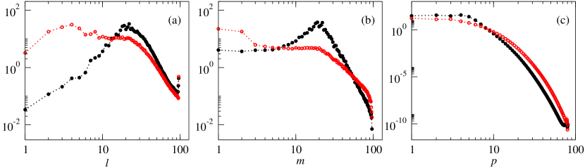
Figure 1: Time-averaged power spectra of kinetic (full circles) and magnetic (empty circles) energy as a function of (a) the harmonic degree $l$, (b) the harmonic order $m$ and (c) the Chebyshev polynomial degree $p$ in the case $\eta=0.65$, $\mathrm{R}=6\times 10^{6}$, $\mathrm{Pr}=1$, $\mathrm{Pm}=2$, $\tau=2000$, $n=2$, $N_{\rho}=3$.

Calculations are considered adequately resolved when the spectral power of kinetic and magnetic energy drops by more than two orders of magnitude from the spectral maximum to the cut-off wavelength as suggested e.g. by Christensen et al. (1999). A range of numerical resolutions has been employed in this study varying from ($N_{r}=61$, $N_{l}=96$) in less demanding cases to ($N_{r}=121$, $N_{l}=144$) in more strongly stratified or turbulent runs. Correspondingly, the physical gridpoints on which non-linear terms are evaluated have been varied up to $N_{r}=121$, $N_{\theta}=216$, $N_{\varphi}=437$. We find that this provides adequate resolution as demonstrated in Figure 1 for a typical dynamo solution.

The pseudo-spectral approach described above is the most common method for solving the fundamental equations of convection-driven flow and electromagnetic induction within a rotating spherical shell filled with an electrically conducting fluid. The approach was pioneered by Glatzmaier (1984) and with appropriate modifications it has been widely used by various groups for modelling convection-driven geo-, Solar, and planetary dynamos. A number of codes based on similar principles have been developed that differ mainly in details such as time stepping methods and treatment of radial dependence with finite differencing and Chebyshev decomposition in $r$ being two popular choices. Early versions of some codes were derived directly from the code of Glatzmaier (1984), including the anelastic ASH code extensively used for Solar simulations (Clune et al., 1999) and the Boussinesq MAG code used for geodynamo simulations (Olson et al., 1999). Other codes including ours were developed independently (e.g. Jones et al., 1995; Tilgner, 1999; Hollerbach, 2000). While it is not feasible to provide here a comprehensive list of existing numerical codes and discuss the numerous variations in actual implementation, we refer to a series of benchmarking papers (Christensen et al., 2001; Jones et al., 2011; Marti et al., 2014; Jackson et al., 2014) and to the reviews (Miesch, 2005; Wicht & Tilgner, 2010) for overview of codes commonly used in the solar context and in the geo-/planetary context, respectively. These references also include discussions of other essentially different numerical approaches of solution. Recent studies related to ours (Fan & Fang, 2014; Karak et al., 2015; Mabuchi et al., 2015; Hotta et al., 2015) use finite difference methods to solve comparable but different sets of equations. Local methods have better parallel efficiency but also inferior accuracy (Tilgner, 1999). They also have difficulties with imposing global boundary conditions for the magnetic field, e.g. all of the above dynamo models use the unphysical radial condition for the magnetic field on the outer surface. They also encounter difficulties in treating spherical geometries, e.g. Fan & Fang (2014) and Karak et al. (2015) consider wedges and not spherical shells. Our code has been developed and optimized independently over a number of years and a large database of Boussinesq results is available for comparison. The current anelastic version of our code is new and perhaps unique among other spectral codes, with the exception of the ASH code, in allowing for a radial dependence of the viscosity and the thermal and magnetic diffusivities. However, the latter facilities have not been used in the present analysis.

2.4 Diagnostic output quantities

We characterise convection and dynamo solutions by their kinetic and magnetic energy and heat transport given by a Nusselt number. The energies can be conveniently split into poloidal and toroidal components, mean and fluctuating components and further into equatorially-symmetric and equatorially-antisymmetric components. We thus obtain a good characterisation of the scales of the convective flow and the multipole structure of dynamos. The mean and fluctuating toroidal and poloidal components of the total kinetic energy $E_{\text{kin}}$ are defined as

$$\bar{E}_{p}=\langle\big{(}\nabla\times(\nabla\bar{v}\times\mbox{\boldmath$r$})\big{)}^{2}/(2\bar{\rho})\rangle, \bar{E}_{t}=\langle\big{(}\nabla r\bar{w}\times\mbox{\boldmath$r$}\big{)}^{2}/(2\bar{\rho})\rangle,$$ (10a)

$$\check{E}_{p}=\langle\big{(}\nabla\times(\nabla\check{v}\times\mbox{\boldmath$r$})\big{)}^{2}/(2\bar{\rho})\rangle, \check{E}_{t}=\langle\big{(}\nabla r\check{w}\times\mbox{\boldmath$r$}\big{)}^{2}/(2\bar{\rho})\rangle,$$ (10b)

where angular brackets $\langle\rangle$ denote averages over the spherical volume of the shell, overlaid lines denote axisymmetric parts and overlaid check marks denote non-axisymmetric parts of a scalar field. The total magnetic energy $E_{\text{magn}}$ can be split in a similar way with components defined as in Equations (10) but with $h$ and $g$ replacing $v$ and $w$ and without the factor $\bar{\rho}^{-1}$ within the angular brackets. The total energies are, of course, the sum of all components. The Nusselt number is defined as the ratio between the values of the luminosity of the convective state $\mathrm{L_{conv}}$ and the luminosity of the basic conduction state $\mathrm{L_{basic}}$,

$$\mathrm{Nu}=\frac{\mathrm{L_{conv}}}{\mathrm{L_{basic}}},\qquad\mathrm{L_{conv}}=-\int_{\partial V(r)}\kappa\bar{\rho}\bar{T}(\partial_{r}S)\mbox{\boldmath$r$}^{2}\sin\theta d\theta d\varphi,\quad\mathrm{L_{basic}}=\frac{4\pi nc_{1}\bar{\rho}(r)^{n}}{\exp(N_{\rho})-1},$$

with the integral taken over a spherical surface $\partial V(r)$ at radius $r$. Apart from quantifying the heat transport of convection, the value of the Nusselt number serves as a convenient proxy for the super-criticality of the convective regime.

Other diagnostic quantities used below are the non-dimensional magnetic Reynolds number, $\mathrm{Rm}=\mathrm{Pm}\sqrt{2E_{\text{kin}}}$, Rossby number, $\mathrm{Ro}=\dfrac{2}{\tau}\sqrt{2E_{\text{kin}}}$, and Lorentz number $\mathrm{Lo}=\dfrac{2}{\tau}\sqrt{2E_{\text{magn}}}$.

2.5 Benchmarking and validation

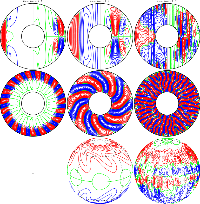
Figure 2: Solutions structures of benchmark cases 1, 2 and 3 (left to right). The first plot in each column shows azimuthally-averaged isocontours of $\overline{u}_{\varphi}$ (left half) and of the streamlines $r\sin\theta(\partial_{\theta}\overline{v})$ (right half) in the meridional plane. The second plot in each column shows isocontours of $u_{r}$ in the equatorial plane. The third plot in each column shows isocontours of $B_{r}$ at $r=r_{o}$.

To validate the new code we present a comparison with the anelastic benchmark simulations recently proposed by Jones et al. (2011). For the comparison we employ an alternative parametrization based on the magnetic rather than viscous diffusion time scale, used in the benchmark models. Our output results from the three benchmark cases defined in Jones et al. (2011) are summarized in Table 1, and selected components of the solution are plotted in Figure 2. The mean values and the means of the deviations computed from the values reported by the four codes participating in (Jones et al., 2011) are also listed in Table 1. We achieve perfect agreement with the benchmark results for the hydrodynamic case and the steady dynamo case, labelled Benchmark 1 and Benchmark 2. Our results for the unsteady dynamo case labeled Benchmark 3 show some insignificant differences from the values reported in Jones et al. (2011). The reason for the discrepancies is the use of imposed 2-fold azimuthal symmetry and lower resolution in our code to reduce computing time.

3 Differential rotation and dynamo action in the buoyancy-dominated regime

It is well known, that as buoyancy forcing becomes significantly larger than the Coriolis force anti-solar differential rotation develops. Such buoyancy-dominated regime was first identified by Gilman (1976) and Gilman & Foukal (1979), and more recently it was studied by Aurnou et al. (2007) and Gastine et al. (2013). More recent studies include the works of (Guerrero et al., 2013a, b) that is closely tailored to the solar case. These studies consistently found that due to vigorous mixing angular momentum is homogenized within the whole volume of the shell, and this leads to a strong retrograde zonal flow in the equatorial region, and thus to the anti-solar type of rotation profile.

3.1 Transition between rotation-dominated and buoyancy-dominated regimes

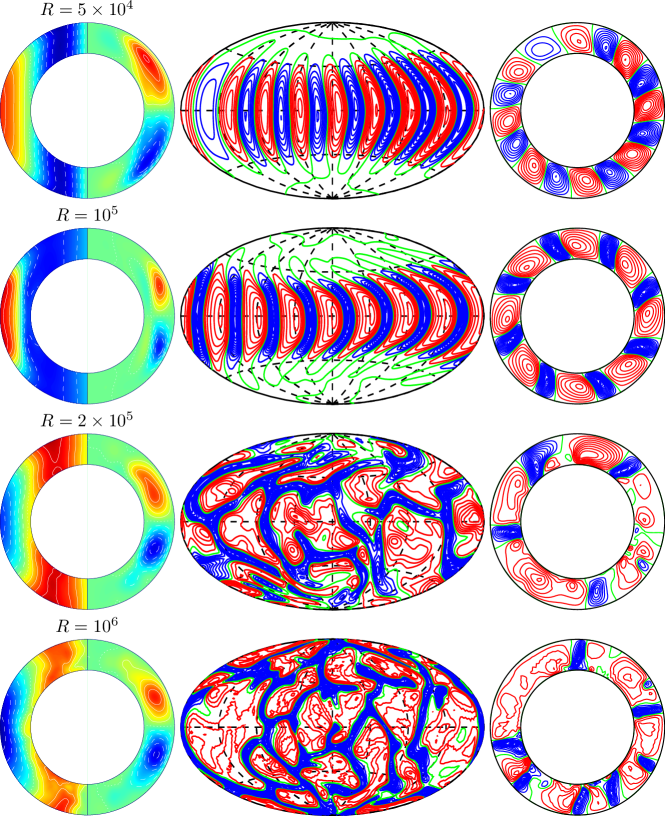
Figure 3: Structures of convection showing the transition to the buoyancy-dominated regime with increasing value of the Rayleigh number as indicated in the plot and $\eta=0.65$, $\mathrm{Pr}=0.3$, $\mathrm{Pm}=3$, $\tau=200$, $n=2$ and $N_{\rho}=3$. The plots in the first column show time- and azimuthally-averaged isocontours of $\overline{u}_{\varphi}$ (left half) and of the streamlines $r\sin\theta(\partial_{\theta}\overline{v})$ (right half) in the meridional plane. The plots in the second column show contours of instantaneous $u_{r}$ on the spherical surface $r=(r_{i}+r_{o})/2$. The plots in the third column show contours of instantaneous $u_{r}$ in the equatorial plane.

Here, we investigate the transition from the rotation-dominated regime to the buoyancy-dominated regime for non-magnetic and magnetic (dynamo) cases. Figure 3 demonstrates the transition from the solar-type to the anti-solar type of differential rotation in a set of cases with increasing value of the Rayleigh number $\mathrm{R}$ and all other parameter values kept fixed. The increase of the Rayleigh number is the most direct approach to the buoyancy-dominated regime as $\mathrm{R}$ is a direct measure of the magnitude of buoyancy forcing. We remark, however, that the buoyancy-dominated regime can also be reached if other control parameters are varied. For instance, a decrease in the Coriolis number $\tau$ at fixed values of the other parameters including $\mathrm{R}$ will equally well bring convection to the buoyancy-dominated regime since $\tau$ is a measure of the Coriolis force. Reaching the regime by variation of the other parameters is also possible but less straightforward. In the case of Figure 3 the transition to the buoyancy-dominated regime happens between $\mathrm{R}=10^{5}$ and $\mathrm{R}=2\times 10^{5}$. The Coriolis-dominated regime is characterized by columnar convection structures that are oriented parallel to the rotation axis and mostly outside the tangent cylinder, the cylinder that touches the inner core at the equator.

In the case of Figure 3, columnar convection has a dominant azimuthal wave number of 8. This number, however, varies as the parameter values are varied. Since even in the strongly chaotic regime the azimuthal wave number of convection remains similar to that near the onset of convection, it is useful to note the study of Busse & Simitev (2014) where the critical onset for this problem has been studied. Differential rotation in the Coriolis-dominated regime is solar-like and geostrophic, i.e. constant on cylindrical surfaces. Meridional circulation is relatively weak but changes from single to two cells in a hemisphere with the increase of $\mathrm{R}$. In this connection we note recent observational results by Zhao et al. (2013) that report two-cell meridional circulation in the solar convection zone.

Convection in the buoyancy-dominated regime for $R>2\times 10^{5}$ in the case of Figure 3 becomes disorganized. Convective columns are broken, and the convection pattern loses its anisotropy with respect to the axis of rotation. Convection, for instance, is now not restricted to the region outside of the tangent cylinder but produces vigorous flows in the polar regions as well. Meridional circulation appears to return to a single-cell pattern but the symmetry with respect to the equatorial plane is lost. This, of course, is due to the fact that the Coriolis force is no longer dominant and the role of rotation is much diminished.

The most notable effect is the sign reversal of the differential rotation that switches from the solar-like to the anti-solar profile. The anti-solar differential rotation remains largely constant on cylinders parallel to the rotation axis. While some conical features are present in the case of Figure 3 they seem to be confined near the surface and appear less significant.

3.2 Effects of magnetic field on differential rotation

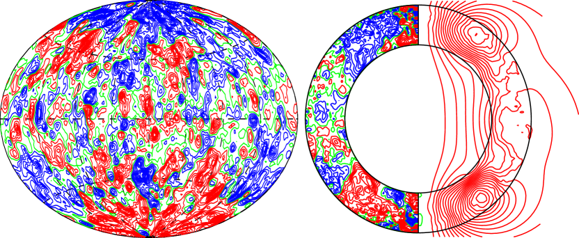
Figure 7: Magnetic field components of the same case as in the right column of Figure 6. The left plot shows contours of $B_{r}$ at $r=1.13+r_{i}$, the right plot shows contours $\overline{B}_{\varphi}$ and meridional field lines.

While solar convection is likely dominated by buoyancy, it is rather challenging to reconcile the anti-solar differential rotation found in the buoyancy-dominated regime with observations. It is well known from helioseismology observations that solar differential rotation is prograde and strongly non-geostrophic (e.g. Thompson et al., 1996). In this situation, magnetic effects may provide one possible mechanism for reversing the anti-solar differential rotation into the solar-like type (Fan & Fang, 2014; Karak et al., 2015; Mabuchi et al., 2015). This is not unreasonable to expect. Indeed, it is well-established that the main effect of self-generated magnetic field on convection is to impede differential rotation. This effect is measured by a strong decrease of mean toroidal kinetic energy in dynamo solutions initially demonstrated by Grote & Busse (2001) and later studied in the parameter space by Simitev & Busse (2005) (see their Fig. 16) and Busse & Simitev (2005) (see their Fig. 7). It has also been investigated by Aubert (2005) and Yadav et al. (2013). To explore the effect of magnetic field on buoyancy-dominated convection as described in the preceding Section, we have performed a systematic comparison between large sets of simulations of non-magnetic convection and of self-sustained dynamos.

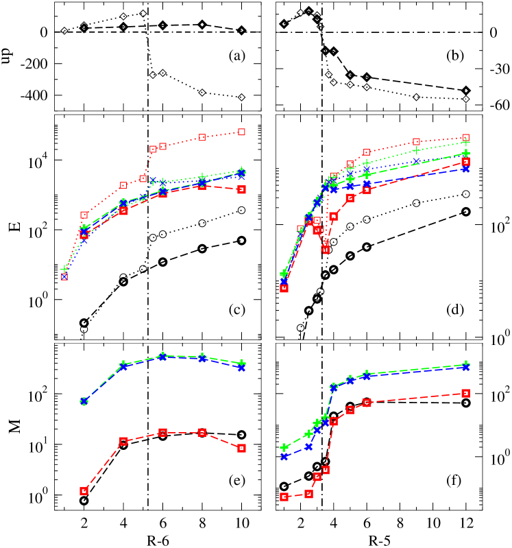
Figure 4: (a,b) Differential rotation at the equator $\overline{u}_{\varphi}(r_{o},\pi/2)$. (c,d) Average kinetic energy densities and (e,f) average magnetic energy densities as functions of the Rayleigh number $\mathrm{R}$ in the cases (a,c,e) for $\eta=0.65$, $\mathrm{Pr}=1$, $\tau=2000$, $n=2$, $N_{\rho}=3$, and in the cases (b,d,f) for $\eta=0.65$, $\mathrm{Pr}=0.5$, $\tau=300$, $n=2$, $N_{\rho}=3$. Nonmagnetic convection cases are denoted by thin symbols in (a,b,c,d). Dynamo cases are denoted by thick symbols in all panels and have $\mathrm{Pm}=2$ in (a,c,e) and $\mathrm{Pm}=6$ in (b,d,f). Black circles, red squares, green pluses and blue crosses denote $\overline{X}_{p}$, $\overline{X}_{t}$, $\tilde{X}_{p}$, $\tilde{X}_{t}$, with $X=E,M$. Vertical dash-dotted lines denote the transition to buoyancy-dominated regime.

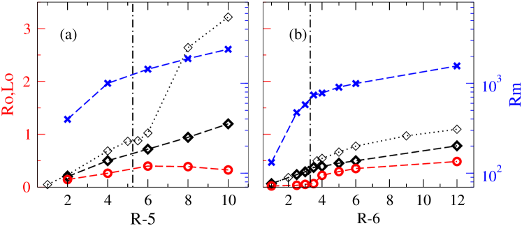
Figure 5: Time-averaged values of the Rossby number Ro (black diamonds) and the Lorentz number Lo (red circles) measured on the left-hand axis and of the magnetic Raynolds number Rm (blue crosses) measured on the right-hand axis. Panel (a) shows the same sequences illustrated in Figure 4(a,c,d) and panel (b) shows the same sequences illustrated in Figure 4(b,d,e). The thin symbols indicate the values of Ro for non-magnetic convection and bold symbols represent the dynamo cases.

Figures 4 and 5 summarize the results of four such sequences of cases with one pair at Prandtl number $\mathrm{Pr}=1$ and Coriolis number $\tau=2000$ and the other pair at somewhat smaller values $\mathrm{Pr}=0.5$ and $\tau=300$. One sequence in each pair is non-magnetic while the other sequence includes a self-generated magnetic field. The specific choice of parameters is motivated by properties of solar convection as discussed below. Time-averaged components of the kinetic and magnetic energy densities are plotted as a function of the increasing Rayleigh number $\mathrm{R}$ for both the convection-only cases and the dynamo cases. The top row of Figure 4 shows the time-averaged value of the differential rotation at the equator on the outer surface of the spherical shell, $\overline{u}_{\varphi}(r_{o},\pi/2)$, and serves as an easily accessible indicator of the type of differential rotation. The transition from the rotation-dominated regime (solar-like rotation) to the buoyancy-dominated regime (anti-solar rotation) is thus easily identified by the sign change of $\overline{u}_{\varphi}(r_{o},\pi/2)$ (marked by a dash-dotted line in Figures 4 and 5). Convection in the absence of magnetic field is characterized by an abrupt as opposed to a gradual increase of both differential rotation and meridional circulation. The total magnetic energy of the self-sustained field is on average an order of magnitude smaller than the kinetic energy, but the magnetic field has a significant effect on both the differential rotation and meridional circulation. In contrast to the non-magnetic case, they are strongly reduced and show no abrupt change in their values.

In the sequences shown in Figure 4(a,c,e) the transition from the solar-like to anti-solar differential rotation is, in fact, suppressed. While we expect that if buoyancy is further increased, i.e. by increasing $\mathrm{R}$, convection will eventually arrive once again at the transition to prograde rotation, we emphasize that the suppression of the transition happens over a large interval of $\mathrm{R}$ comparable to the interval between the onset of convection and the solar-antisolar transition itself.

In the sequences shown in Figure 4(b,d,f) the suppression of the solar-antisolar transition is not observed, even though the effects of decreasing differential rotation and meridional circulation are visible. This difference illustrates other important parameter dependences, primarily those on the Prandtl and the Coriolis numbers, $\mathrm{Pr}$ and $\tau$, respectively. In the region of low values of Prandtl and Coriolis numbers convection is known to be rather different from columnar convection in that it takes the form of an equatorial belt of large cells attached near the outer surface of the spherical shell (Ardes et al., 1997; Busse & Simitev, 2004). Differential rotation generated by equatorially-attached convection is typically less affected by the braking effect of the magnetic field (Simitev & Busse, 2005).

Figure 5 shows the values of the Rossby, Lorentz and magnetic Reynolds number in dependence of the Rayleigh number of the same sequences as shown in Figure 4. The transition from rotation-dominated to buoyancy-dominated convection happens at about $\mathrm{Ro}=1$ in the sequence of Figure 4(a,c,e) and at about $\mathrm{Ro}=0.5$ in the sequence of Figure 4(b,d,f). These values are similar to the ones reported by Gastine et al. (2014), Karak et al. (2015) and Mabuchi et al. (2015) but a weak dependence on the Prandtl and the Coriolis numbers appears to exist. The dynamo effects do not appear to affect the value of the Rossby number for transition in agreement with Karak et al. (2015) and Mabuchi et al. (2015).

Further notable effects of the magnetic field are summarized in Table 2. These effects are illustrated in terms of one selected strongly chaotic case discussed below.

3.3 Structure and dynamics of convective flows and magnetic fields in the buoyancy-dominated regime

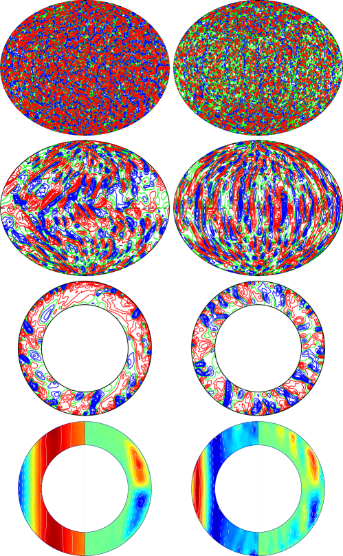
Figure 6: Comparison between non-magnetic convection (left) and dynamo (right) at identical parameter values $\eta=0.65$, $\mathrm{Pr}=1$, $\tau=2000$, $\mathrm{R}=10^{7}$, $n=2$, $N_{\rho}=3$ and for the dynamo $\mathrm{Pm}=2$. Plots in the first row show $u_{r}$ at $r=0.95+r_{i}$, plots in the second row show $u_{r}$ at $r=0.3+r_{i}$, plots in the third row show $u_{r}$ in the equatorial plane, plots in the fourth row show isocontours of the differential rotation $\overline{u}_{\varphi}$ (left half) and of the streamlines $r\sin\theta(\partial_{\theta}\overline{v})$ (right half) in the meridional plane. The plots in the first three rows are instantaneous snapshots, while the density plots in the fourth row are time-averaged.

Figure 6 shows a comparison of the spatial structures of the convective flow of a non-magnetic case and those of a self-sustained magnetic dynamo case at identical parameter values $\eta=0.65$, $\mathrm{Pr}=1$, $\tau=2000$, $\mathrm{R}=10^{7}$, $n=2$, $N_{\rho}=3$ and for the dynamo solution $\mathrm{Pm}=2$. At $\eta=0.65$ the shell thickness is slightly thicker than the thickness of the solar convection zone and is selected for ease of numerical simulation. The typical size of convective structures is related to the thickness of the shell and thus thinner shells require spherical harmonics decomposition of higher order and degree to resolve the angular structure of the flow. The value $Pr=1$ is appropriate in the sense that turbulent mixing tends to homogenize the flow and molecular diffusivities are replaced by effective turbulent diffusivities of similar magnitude. At $\tau=2000$ the Coriolis number is moderately but not excessively large reflecting the model assumption that the flow in the deep convection zone is buoyancy rather than rotation dominated. The values of the polytropic index $n=2$ is adequate, while the value of the density scale height $N_{\rho}=3$ is much lower than estimated for the solar convection zone. However, increasing, $N_{\rho}$ much beyond 5 becomes computationally very demanding. Finally, the value of the Rayleigh number has been selected such that the non-magnetic convection case is located in the buoyancy-dominated regime, the onset of which is at $\mathrm{R}=5.2\times 10^{6}$ for these parameter values.

In the case of non-magnetic convection shown in the right column of Figure 6 differential rotation is in anti-solar direction. It is strongly geostrophic i.e. constant on cylinders parallel to the rotation axis. Differential rotation is monotonously increasing towards the outer surface of the spherical shell. Note that this is also true for solar-like differential rotation in the rotation dominated regime. The structure of the flow changes significantly with radius. The first two rows of Figure 6 show isocontours of the radial velocity near the surface and somewhat below mid depth within the spherical shell. The flow near the surface is a patchwork of small-scaled up- and down-wellings distributed in a very chaotic pattern over the full surface of the spherical shell. No visible structure can be discerned and the location of the convective cells changes chaotically in time (not shown). The scale of the convective structures increases in depth and near the equator elongated convective cells tilted clockwise in the northern hemisphere and tilted anticlockwise in the southern hemisphere are found. On average this equatorial pattern drifts in the retrograde direction carried away by the strong anti-solar differential rotation. The so described radial structure is also evident in the contour lines of the radial velocity in the equatorial plane plotted in the third row of 6. Finally, the meridional flow takes the form of two large circulations in poleward direction at the surface of the shell. The meridional circulations are nearly strictly mirror-symmetric with respect to the equatorial plane. This and the symmetry of the differential rotation are remarkable large-scale coherent features of this otherwise very chaotic solution.

As noted above the magnetic energy is significantly lower than the kinetic energy of the flow. The influence of the magnetic field on convection, however, in the dynamo case shown in the left column of Figure 6 is quite remarkable. The most notable effect is, of course the reversal of the direction of differential rotation from the anti-solar to solar-like type. A further remarkable difference is that the maximum of the differential rotation occurs in the depth of the spherical shell rather than at the surface as is always observed in the case of non-magnetic convection. This is potentially a significant effect as it means that there is a negative gradient of differential rotation in the subsurface layer of the shell.

In the magnetic case the structure of the flow also changes significantly with radius. The first two rows of Figure 6 show isocontours of the radial velocity at the same radial values as in the non-magnetic case. The flow near the surface is a again a patchwork of small-scaled up- and down-wellings distributed in a very chaotic pattern. No visible structure can be discerned and the location of the convective cells changes chaotically in time (not shown). An important effect of the magnetic field is that in the magnetic dynamo case convection appears to be stronger in the polar regions rather than outside the tangent cylinder. The main difference, however, appears in depth. Large scale convective columns arranged in a cartridge belt pattern within the tangent cylinder and spanning both hemispheres to about mid latitudes are clearly visible. The columns drift in the prograde direction due to the solar-like differential rotation. This is also a significant observation because it indicates that very little may be inferred for the structure of deep convection from observations of near surface flows. In particular, it is not known whether large scale convective columns exist in the deep solar convection zone or not. Our results indicate large scale convective columns hidden from view by much smaller-scale chaotic convection with no discernible structure is a likely dynamical possibility. Finally, the meridional flow of the magnetic dynamo case appears rather disorganized with a number of smaller scale circulations appearing in both hemispheres as shown in the bottom row of Figure 6.

The structure of the generated magnetic field in the dynamo case is shown in Figure 7. The magnetic field has a large-scale dipole component emerging from a patchwork of small scale magnetic features. The dipole is mainly supported by strong polar magnetic flux tubes in the polar region, which in turn are due to the relatively strong polar convection. The predominant polarity is less clear in the equatorial region where the magnetic field structures are smaller in scale and of both polarities. The dipole solution is non-oscillating. Unfortunately, we have not been able to locate oscillating dynamos in this regime and to observe the direction of dynamo wave propagation. This is left for future studies.

4 Remarks on anelastic dynamos in the rotation-dominated regime

While the attention in this paper is focussed on dynamo effects near the transition from rotation-dominated to buoyancy-dominated convection, in this section we wish to demonstrate that conical profiles of differential rotation as well as regular and persistent dynamo oscillations can be found in the parameter space of our minimal convection-driven dynamo model without recourse to additional modelling assumptions. We also take the opportunity to elucidate some of the points made about buoyancy-dominated dynamos above by comparison with features in the rotation-dominated regime.

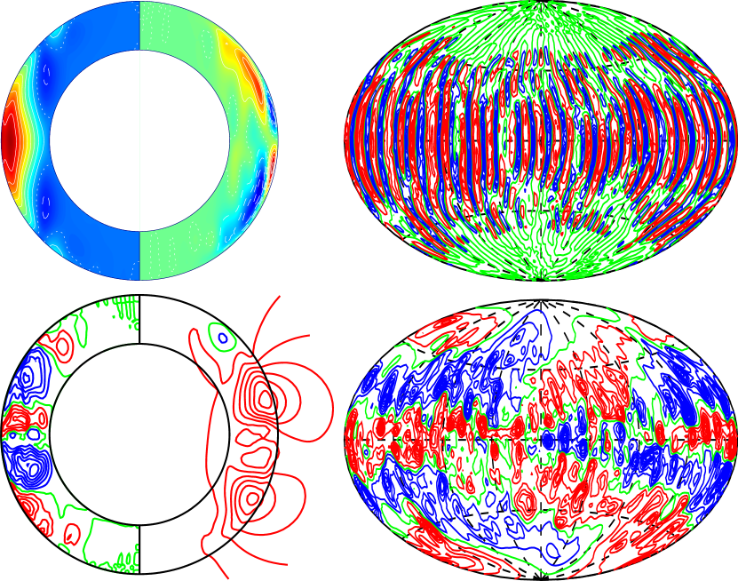
Figure 8: Flow and field structures in the case $\eta=0.65$, $\mathrm{Pr}=1$, $\tau=2\times 10^{3}$, $\mathrm{R}=1.8\times 10^{6}$, $\mathrm{Pm}=8$, $n=2$, $N_{\rho}=3$ with no-slip condition on the inner boundary. The top left plot shows time-averaged isocontours of the differential rotation $\overline{u}_{\varphi}$ (left half) and of the streamlines $r\sin\theta(\partial_{\theta}\overline{v})$ (right half) in the meridional plane. The top right plot shows contours of instantaneous $u_{r}$ at $r=0.5+r_{i}$. The bottom left plot shows contours of instantaneous $\overline{B}_{\varphi}$ (left half) and meridional field lines (right half). The bottom right plot shows contours of instantaneous $B_{r}$ at $r=1.13+r_{i}$.

Perhaps the only clear example of a conical profile of differential rotation in a single-layer simulation with spherically-symmetric boundary conditions is that reported in the work of Brun & Toomre (2002). However, these authors use subgridscale parametrisation of diffusivities which clearly affects results. Following Miesch et al. (2006), the majority of models that report conical profiles seem to impose a non-zero latitudinal gradient of entropy as their bottom boundary condition (e.g. Fan & Fang, 2014) or to include anisotropic heat conductivity (e.g. Karak et al., 2015) or a stably stratified layer at the bottom of the convection zone (e.g. Mabuchi et al., 2015) all of which increase the baroclinicity and induce conical profiles. In this context, Figure 8 shows an example of differential rotation with some conical features in the lower part of the convection zone, obtained in our minimal self-consistent formulation of the problem. The parameter values of this run are the same as those for the sequence of cases reported in Figure 4(a,c,e), with a value of the Rayleigh number that places it in the rotation-dominated regime, and a somewhat larger value of $\mathrm{Pm}$ which is known to promode stronger dipolar fields (Simitev & Busse, 2005). This run differs from the latter sequence only in that it uses a no-slip velocity condition on the inner spherical boundary. Convection in the polar regions is weak if not fully absent. Convective flows are confined outside of the tangent cylinder and this is where the dynamo process is also located resulting in a magnetic field that is strong near the equator and at midlatitudes but weak in the polar regions. We wish to contrast this situation with the situation discussed in connection to the dynamo case presented in Figures 6 and 7. This comparison makes it rather obvious that in the latter case vigorous convection in the polar regions gives rise to strong magnetic field in the same regions. The dynamo shown in Figure 8 is an oscillatory dynamo and the comparison with the case of Figure 7 elucidates the reasons why the latter is non-oscillatory. While in the case of Figure 8 both the magnetic field and the differential rotation achieve their maxima in the same region (the equatorial region), in the case of Figure 7 the regions where the maximal amplitude of the magnetic field and of the differential rotation occur do not coincide which is detrimental to $\alpha\Omega$ oscillations (Busse & Simitev, 2006; Warnecke et al., 2014).

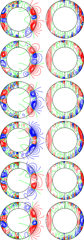
Figure 9: One period of dipolar oscillations in the case $\eta=0.65$, $\mathrm{Pr}=1$, $\tau=2\times 10^{3}$, $\mathrm{R}=2.5\times 10^{6}$, $\mathrm{Pm}=4$, $n=2$, $N_{\rho}=3$ with no-slip condition on the inner boundary. Time between plots is $\Delta t=0.09$ staring at $t_{0}=96.8174$ in the time series shown in figure 10. The first row shows contours $\overline{B}_{\varphi}$ to the left and meridional field lines to the right. The second row shows contours $\overline{u}_{\varphi}$ to the left and the streamlines $r\sin\theta(\partial_{\theta}\overline{v})$ to the right all in the meridional plane.

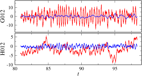
Figure 10: Regular and persistent dipole-dominated oscillations shown in the time series of the axisymmetric toroidal coefficients $G_{0}^{1}$ (red) and $G_{0}^{2}$ (blue) and the axisymmetric poloidal coefficients $H_{0}^{1}$ (red) and $H_{0}^{2}$ (blue) describing the main dipolar and quadrupolar contributions in the spherical harmonic expansion of the magnetic field in the case shown in figure 9.

To illustrate the oscillations in question, we present in Figure 9 one period of a predominantly dipolar dynamo wave. The parameter values of this run are identical to the cases shown in Figure 8 except for a slightly larger value of the Rayleigh number which helps to make the oscillations more regular. The dynamo wave is driven by the $\alpha\Omega$ mechanism first proposed by Parker (1955) and later confirmed in three-dimensional simulations by Busse & Simitev (2006), see also (Simitev & Busse, 2012a; Schrinner et al., 2012; Warnecke et al., 2014). The dynamo wave propagates in the direction of the poles. This case shows similar conical features of the differential rotation profile, and Figure 9 also illustrates their variations in time. Figure 10 shows the dominant dipolar and quadrupolar components of the magnetic field represented by time series of the appropriate coefficients in the spherical harmonic expansions of the toroidal and poloidal scalars of the magnetic field. The time series show that the oscillations are very regular and persistent over the course of the simulation and that the dipole is dominant.

We wish to conclude this section with the remark that the parameter space of the minimal model formulation seems to merit further investigation especially in the case when self-generated magnetic fields are present.

5 Conclusion

We have presented in this paper several sets of convective dynamo simulations in density-stratified rotating spherical fluid shells based on a physically consistent anelastic model with a minimum number of parameters. The computations are performed using a new simulation code that is also presented here for the first time along with code validation results against published benchmark solutions. We demonstrate that conical differential rotation profiles and persistent regular dynamo oscillations can be obtained in the parameter space of this minimal formulation without recourse to additional modelling assumptions. The main focus of the work is placed on extending the dynamo simulations into a “buoyancy-dominated” regime where the buoyancy forcing is dominant while the Coriolis force is no longer balanced by pressure gradients and where strong anti-solar differential rotation develops as a result. The dynamo solutions are compared to identical sets of non-magnetic convection solutions to reveal the effects of the self-sustained magnetic field on convection in general and on the differential rotation in particular. The most significant results are summarized in Table 2 and below we discuss some similarities between our solutions and solar and stellar convection.

We also wish to compare our results to studies on a similar topic reported in the recent literature, in particular the works of Fan & Fang (2014), Karak et al. (2015) and Mabuchi et al. (2015) where dynamo simulations are reported and of Gastine et al. (2013) and Hotta et al. (2015) where hydrodynamic simulations are reported. Before we comment on similarities and differences in solutions, we wish to point out that with the exception of the model considered by Gastine et al. (2013), the models considered by the other groups have significant and essential differences compared to ours. The models of Hotta et al. (2015), Karak et al. (2015) and Mabuchi et al. (2015) are fully compressible models in contrast to our anelastic approximation. Hotta et al. (2015) use artificially enhanced viscosity, a radius dependent cooling term and are interested mainly in the properties of the near-surface convection layer. The model of Mabuchi et al. (2015) consists of two layers – a stably stratified layer surrounded by a convective envelope. The models of Fan & Fang (2014) and Karak et al. (2015) consider wedges, i.e. partial spherical shells, and are not fully spherical, so polar convection is effectively not represented in their solutions. This partly explains why they find oscillatory dynamos. Conical differential rotation profiles are promoted in the latter four models due to the inclusion of secondary physical effects: Fan & Fang (2014) impose a latitudinal entropy gradient as a bottom boundary condition, Fan & Fang (2014), Hotta et al. (2015) and Karak et al. (2015) include radial variation in diffusivities and parametrisations of unresolved scales. Numerical implementations also differ – all codes except that of Gastine et al. (2013) are based on finite-difference methods while ours is pseudo-spectral. An artificial radial magnetic field condition is imposed on the outer boundary in these studies which may significantly distort dynamo effects. Despite the differences in modelling strategy, it is significant that we find a number of similarities in our simulations. This increases the confidence in the robustness of the reported results.

Oscillations obtained in dynamos generated within the rotation-dominated regime with few exceptions (Warnecke et al., 2014), appear to always travel in the poleward direction much like illustrated in Figure 9. For references see (Busse & Simitev, 2006; Simitev & Busse, 2012a), and also (Schrinner et al., 2012). There is some evidence that dynamo waves can travel towards the equator when a negative radial gradient of the differential rotation profile exists (Simitev & Busse, 2012b), and when in addition to the latter the $\alpha$-effect, proportional to $-(\nabla\times\mbox{\boldmath$u$})\cdot\mbox{\boldmath$u$}+(\nabla\times\mbox{\boldmath$B$})\cdot\mbox{\boldmath$B$}/\bar{\rho}$, is positive (negative) in the northern (southern) hemisphere (Warnecke et al., 2014). This evidence supports an early analysis by Yoshimura (1975). While we commonly find dipolar oscillations in the rotation-dominated regime, our dynamos in the buoyancy-dominated regime do not oscillate. This is in contrast to the results of Fan & Fang (2014) and Karak et al. (2015) which may be attributed to the absence of polar convection in their simulations due to the absence of conical polar sections used in their geometrical configuration. On the other hand, we agree with Mabuchi et al. (2015) who use a full spherical shell and find that dynamos with anti-solar rotation are predominantly dipolar and non-oscillatory. Despite being relatively weak the self-sustained magnetic fields in the buoyancy-dominated regime reported in the present study are able to reverse the direction of differential rotation from anti-solar to solar-like. From the perspective of oscillations, it is significant that we find that differential rotation attains a maximum inside the shell and that a negative radial gradient is persistently maintained in the near-surface layer. This may facilitate equatorward dynamo wave propagation in the buoyancy-dominated regime. The differential rotation in our buoyancy-dominated dynamos, e.g. Figure 6, has a cylindrical profile, in contrast to the more conical profiles reported by Fan & Fang (2014) Karak et al. (2015) and Mabuchi et al. (2015). This difference is almost certainly caused by the fact that a non-zero latitudinal gradient of entropy is imposed as a bottom boundary condition by Fan & Fang (2014), that an anisotropic heat conductivity is used by Karak et al. (2015), and that a stably stratified layer at the bottom of the convection zone is present in (Mabuchi et al., 2015).

We find that the dynamo-generated magnetic field can suppress the transition from the solar-like to the antisolar-like rotation profile thus confirming similar findings reported by Fan & Fang (2014) Karak et al. (2015) and Mabuchi et al. (2015). In this case the convection is significantly stronger near the poles than in the equatorial region, leading to a predominantly dipolar dynamo where both the toroidal and the poloidal fluxes are stronger in the polar regions compared to equatorial regions. Such dynamo regime with concentration of magnetic field in the polar regions may explain the observations of polar starspots in young solar-type stars which exhibit reduced but still the solar-type differential rotation (Brown et al., 2014), also see (Yadav et al., 2015). While starspots reduce locally the vigour of convection in the near surface layer of the convection zone, sufficiently strong convection in depth is required to generate magnetic fields that are large enough to cause starspots in the first place. Our calculations do not have sufficient resolution to resolve strongly turbulent stellar near surface layers.

Our simulations confirm the findings of Gastine et al. (2013) and Hotta et al. (2015) that different regimes of convection occur in the inner and at the outer part of the spherical shell simultaneously such that organized geostrophic convection columns are hidden below a near-surface layer of well-mixed highly-chaotic convection. Both of the latter studies are non-magnetic and the work of Hotta et al. (2015) reports simulations in the rotation-dominated regime only. The model of Gastine et al. (2013) is rather similar to ours and it is one of the aims of the present paper to extend their analysis through considerations of dynamo effects. On the Sun small scale turbulent convection is clearly observable in the subsurface layer of the solar convection zone while simulations inevitably find some columnar structures. Evidence of different convection morphology as a function of radius is significant because it provides a bridge between observations and simulations. The deeper large-scale organized convection columns are likely to play important role in the solar dynamo and its magnetic cycles.

Appendix A Spectral projection of the toroidal-poloidal governing equations

Scalar equations for $v$ and $w$ are obtained, and effective pressure gradients are eliminated by taking $\hat{\mbox{\boldmath$r$}}\cdot\nabla\times\nabla\times$ and $\hat{\mbox{\boldmath$r$}}\cdot\nabla\times$ of Equation (2b). Similarly, equations for $h$ and $g$ are obtained by taking $\hat{\mbox{\boldmath$r$}}\cdot\nabla\times$ and $\hat{\mbox{\boldmath$r$}}\cdot$ of Equation (2d). The scalar unknowns $v$, $w$, $h$, $g$ and $S$ are then expanded in Chebychev polynomials $T_{p}$ in the radial direction $r$, and in spherical harmonics $Y_{l}^{m}$ in the angular directions $(\theta,\varphi)$ as shown in Equation (9). After a standard Galerkin projection procedure in the angular directions $(\theta,\varphi)$ the following set of partial differential equations for the spectral expansion coefficients $\{v_{l}^{m}(r,t),w_{l}^{m}(r,t),h_{l}^{m}(r,t),g_{l}^{m}(r,t),S_{l}^{m}(r,t)\;:\;l=1\ldots{L_{\text{max}}},\,m=-l\ldots l\}$ is obtained

$$\partial_{t}{w_{l}^{m}}-\left(\partial_{r}^{2}+\frac{4}{r}\partial_{r}{}+\frac{2-l(l+1)}{r^{2}}\right)w_{l}^{m}=-\zeta^{n}\Xi_{2}w_{l}^{m}$$ (A1a)

$$\hskip 14.22636pt-\frac{1}{l(l+1)}\zeta^{n}\left[\hat{\mbox{\boldmath$r$}}\cdot\nabla\times\Bigg{(}\Xi_{1}\partial_{r}{\mbox{\boldmath$v$}}+\tau\Big{(}\hat{\mbox{\boldmath$k$}}\times\frac{\mbox{\boldmath$v$}}{\zeta^{n}}\Big{)}+\left(\Big{(}\nabla\times\frac{\mbox{\boldmath$v$}}{\zeta^{n}}\Big{)}\times\frac{\mbox{\boldmath$v$}}{\zeta^{n}}\right)-\frac{1}{\zeta^{n}}(\nabla\times\mbox{\boldmath$B$})\times\mbox{\boldmath$B$}\Bigg{)}\right]_{l}^{m},$$

$$\partial_{t}{}\mathcal{D}_{l}v_{l}^{m}-\mathcal{D}_{l}\mathcal{M}_{l}v_{l}^{m}=-\mathcal{E}_{l}v_{l}^{m}-\frac{1}{r^{2}}\Xi_{3}l(l+1)v_{l}^{m}-\frac{2}{3}n^{2}\frac{(\zeta^{\prime})^{2}}{\zeta^{n+2}}\frac{l(l+1)}{r^{2}}v-\frac{\mathrm{R}}{\mathrm{Pr}}\frac{1}{r^{3}}S_{l}^{m}$$ (A1b)

$$\hskip 28.45274pt+\frac{r}{l(l+1)}\left[\hat{\mbox{\boldmath$r$}}\cdot\nabla\times\nabla\times\Bigg{(}\Xi_{1}\partial_{r}{\mbox{\boldmath$v$}}+\tau\Big{(}\hat{\mbox{\boldmath$k$}}\times\frac{\mbox{\boldmath$v$}}{\zeta^{n}}\Big{)}+\left(\Big{(}\nabla\times\frac{\mbox{\boldmath$v$}}{\zeta^{n}}\Big{)}\times\frac{\mbox{\boldmath$v$}}{\zeta^{n}}\right)-\frac{1}{\zeta^{n}}(\nabla\times\mbox{\boldmath$B$})\times\mbox{\boldmath$B$}\Bigg{)}\right]_{l}^{m},$$

$$\partial_{t}{}S_{l}^{m}-\frac{1}{\mathrm{Pr}}\mathcal{M}_{l}S_{l}^{m}=\frac{1}{\mathrm{Pr}}(n+1)\frac{\zeta^{\prime}}{\zeta}\partial_{r}{}S_{l}^{m}-\left[\frac{1}{\zeta^{n}}\nabla\cdot(S\mbox{\boldmath$v$})\right]_{l}^{m}$$ (A1c)

$$\hskip 85.35826pt+\left[\frac{c_{1}\mathrm{Pr}}{\mathrm{R}\zeta}\Big{(}Q_{v}+\frac{1}{\mathrm{Pr}_{m}\zeta^{n}}(\nabla\times\mbox{\boldmath$B$})^{2}\Big{)}\right]_{l}^{m}-\frac{l(l+1)}{r}\frac{v_{l}^{m}}{\zeta^{n}}\frac{1}{r^{2}}\frac{1}{\zeta^{n+1}}\frac{c_{1}nd\zeta(r_{i})^{n}\zeta(r_{o})^{n}}{\zeta(r_{o})^{n}-\zeta(r_{i})^{n}},$$

$$\partial_{t}{}h_{l}^{m}-\frac{1}{\mathrm{Pm}}\left(\partial_{r}^{2}-\frac{l(l+1)}{r^{2}}\right)h_{l}^{m}=\frac{r^{2}}{l(l+1)}\left[\hat{\mbox{\boldmath$r$}}\cdot\nabla\times\Big{(}\frac{\mbox{\boldmath$v$}}{\zeta^{n}}\times\mbox{\boldmath$B$}\Big{)}\right]_{l}^{m},$$ (A1d)

$$\partial_{t}{}g_{l}^{m}-\frac{1}{\mathrm{Pm}}\left(\partial_{r}^{2}-\frac{l(l+1)}{r^{2}}\right)g_{l}^{m}=\frac{r^{2}}{l(l+1)}\left[\hat{\mbox{\boldmath$r$}}\cdot\nabla\times\nabla\times\Big{(}\frac{\mbox{\boldmath$v$}}{\zeta^{n}}\times\mbox{\boldmath$B$}\Big{)}\right]_{l}^{m},$$ (A1e)

where the following operators are defined

$$\mathcal{M}_{l}=\frac{1}{r^{2}}\big{(}\partial_{r}{}r^{2}\partial_{r}{}-l(l+1)\big{)}=\partial_{r}^{2}+\frac{2}{r}\partial_{r}{}-\frac{l(l+1)}{r^{2}},$$

$$\mathcal{D}_{l}=\left(\left(\frac{1}{\zeta^{n}}\right)^{\prime}\Big{(}\partial_{r}{}+\frac{1}{r}\Big{)}+\frac{1}{\zeta^{n}}\mathcal{M}_{l}\right),$$

$$\mathcal{E}_{l}=\left(\Xi_{2}^{\prime}\Big{(}\partial_{r}{}+\frac{1}{r}\Big{)}+\Xi_{2}\mathcal{M}_{l}\right),$$

and the following notation of some radial functions is used for brevity

$$\Xi_{1}(r)=\frac{1}{\zeta^{n}}\frac{n\zeta^{\prime}}{\zeta},\qquad\Xi_{2}(r)=\frac{1}{\zeta^{n}}\left(\frac{3}{r}\frac{n\zeta^{\prime}}{\zeta}+\left(\frac{n\zeta^{\prime}}{\zeta}\right)^{\prime}\right),\qquad\Xi_{3}(r)=\frac{1}{\zeta^{n}}\left(\frac{1}{r}\frac{n\zeta^{\prime}}{\zeta}-\left(\frac{n\zeta^{\prime}}{\zeta}\right)^{\prime}\right).$$

The expression for the viscous dissipation in Equation (A1c) is

$$Q_{v}=Q_{v}^{(1)}+Q_{v}^{(2)},$$

$$Q_{v}^{(1)}=2\left(\partial_{r}{\frac{v_{r}}{\zeta^{n}}}\right)^{2}-\frac{2}{3}\left(\frac{v_{r}}{\zeta^{n}}\frac{n}{\zeta}\partial_{r}{\zeta}\right)^{2}+2\left(\partial_{r}{\frac{v_{r}}{\zeta^{n}}}+\frac{v_{r}}{\zeta^{n}}\Big{(}\frac{n}{\zeta}\partial_{r}{\zeta}+\frac{1}{r}\Big{)}+q_{v}^{(1)}\right)^{2}+2\left(q_{v}^{(1)}+\frac{1}{r}\frac{v_{r}}{\zeta^{n}}\right)^{2},$$

$$Q_{v}^{(2)}=\left(2\partial_{r}{\frac{v_{\theta}}{\zeta^{n}}}-\Big{[}\nabla\times\frac{\mbox{\boldmath$v$}}{\zeta^{n}}\Big{]}_{\varphi}\right)^{2}+\left(2\partial_{r}{\frac{v_{\phi}}{\zeta^{n}}}+\Big{[}\nabla\times\frac{\mbox{\boldmath$v$}}{\zeta^{n}}\Big{]}_{\theta}\right)^{2}+\Big{(}2q_{v}^{(2)}+\Big{[}\nabla\times\frac{\mbox{\boldmath$v$}}{\zeta^{n}}\Big{]}_{r}\Big{)}^{2},$$

$$q_{v}^{(1)}=\frac{\cos\theta}{r\sin\theta}\frac{v_{\theta}}{\zeta^{n}}+\frac{1}{r\sin\theta}\partial_{\varphi}{\frac{v_{\varphi}}{\zeta^{n}}},\qquad q_{v}^{(2)}=-\frac{\cos\theta}{r\sin\theta}\frac{v_{\varphi}}{\zeta^{n}}+\frac{1}{r\sin\theta}\partial_{\varphi}{\frac{v_{\theta}}{\zeta^{n}}}.$$

Finally, square brackets with a subscript (and superscript) as in $[\cdot]_{\varphi}$ or $[\cdot]_{l}^{m}$ denote a component of a vector or an appropriate coefficient in a spherical harmonic expansion, respectively.

Solution of Equations (A1) proceeds as described in Section 2.3.

Table 1: Comparison with the benchmark solutions reported by Jones et al. (2011). The values labelled “Mean $\pm$ Mean Deviation” are the respective means and the means of the deviations computed from the values reported by the four codes participating in (Jones et al., 2011).

	Benchmark 1:	Benchmark 2:	Benchmark 3:
	Hydrodynamic convection	Steady dynamo	Unsteady dynamo
$\eta$	0.35	0.35	0.35
$n$	2	2	2
$N_{\rho}$	5	3	3
$\mathrm{Pr}$	1	1	2
$\mathrm{Pm}$	1	50	2
$\tau$	2000	1000	$4\times 10^{4}$
$\mathrm{R}$	351806	$8\times 10^{4}$	$2.5\times 10^{7}$
$N_{r}$ / $N_{r}$	129 / 129	129 / 129	111 / 111
$N_{l}$ / $N_{\theta}$	128 / 128	128 / 128	120 / 144
$N_{m}$ / $N_{\varphi}$	129 / 257	129 / 257	61 / 73
Timestep	$4\times 10^{-6}$	$1\times 10^{-6}$	$1\times 10^{-7}$
$E$	81.87991	$4.19405\times 10^{5}$	$2.32730\times 10^{5}$
Mean $\pm$ Mean Dev.	$81.680\pm 0.245$	$(4.186\pm 0.013)\times 10^{5}$	$(2.317\pm 0.014)\times 10^{5}$
$\overline{E}_{p}$	0.02201	53.0100	100.40
Mean $\pm$ Mean Dev.	$0.0220\pm 0.0001$	$52.90\pm 0.15$	111.75 $\pm$ 3.75
$\overline{E}_{t}$	9.37598	$6.01725\times 10^{4}$	$1.81399\times 10^{4}$
Mean $\pm$ Mean Dev.	$9.3568\pm 0.0282$	$(6.001\pm 0.018)\times 10^{4}$	$(1.355\pm 0.008)\times 10^{4}$
$M$	–	$3.20172\times 10^{5}$	$2.58012\times 10^{5}$
Mean $\pm$ Mean Dev.		$(3.194\pm 0.088)\times 10^{5}$	$(2.413\pm 0.023)\times 10^{5}$
$\overline{M}_{p}$	–	$1.69650\times 10^{4}$	$2.91155\times 10^{4}$
Mean $\pm$ Mean Dev.		$(1.692\pm 0.005)\times 10^{4}$	$(2.155\pm 0.070)\times 10^{4}$
$\overline{M}_{t}$	–	$2.41185\times 10^{5}$	$1.17292\times 10^{4}$
Mean $\pm$ Mean Dev.		$(2.412\pm 0.028)\times 10^{5}$	$(0.948\pm 0.003)\times 10^{4}$
Luminosity	4.19886	11.50302	42.50992
Mean $\pm$ Mean Dev.	$4.19886\pm 3\times 10^{-6}$	$11.503\pm 4\times 10^{-5}$	$42.75\pm 0.15$

Table 2: Summary of the effects of self-sustained magnetic field and comparison with non-magnetic convection.

Non-magnetic convection	Dynamo
Monotonic increase/decrease of differential rotation towards the outer surface in solar/antisolar cases.	Differential rotation attains a maximum inside shell and a subsurface decrease.
Retrograde differential rotation in buoyancy-dominated regime.	Differential rotation reversed from antisolar to solar-like.
No columnar structure at depth.	Convective columns visible in depth.

References

- Ardes et al. (1997) Ardes, M., Busse, F., & Wicht, J. 1997, Physics of the Earth and Planetary Interiors, 99, 55
- Aubert (2005) Aubert, J. 2005, Journal of Fluid Mechanics, 542, 53
- Aurnou et al. (2007) Aurnou, J., Heimpel, M., & Wicht, J. 2007, Icarus, 190, 110
- Braginsky & Roberts (1995) Braginsky, S. I., & Roberts, P. H. 1995, Geophysical & Astrophysical Fluid Dynamics, 79, 1
- Brown et al. (2014) Brown, C., Carter, B., Marsden, S., & Waite, I. 2014, in IAU Symposium, Vol. 302, IAU Symposium, 148–149
- Browning et al. (2006) Browning, M. K., Miesch, M. S., Brun, A. S., & Toomre, J. 2006, The Astrophysical Journal Letters, 648, L157
- Brun & Toomre (2002) Brun, A., & Toomre, J. 2002, The Astrophysical Journal, 570, 865
- Brun et al. (2014) Brun, A. S., García, R. A., Houdek, G., Nandy, D., & Pinsonneault, M. 2014, Space Sci. Rev., arXiv:1503.06742
- Busse (1970) Busse, F. H. 1970, ApJ, 159, 629
- Busse (1973) Busse, F. H. 1973, Astronomy and Astrophysics, 28, 27
- Busse et al. (2003) Busse, F. H., Grote, E., & Simitev, R. D. 2003, in Fluid Mech. Astrophys. Geophys. Series vol. 11: ”Earth’s Core and Lower Mantle”, ed. J. C. A., S. A. M., & Z. K. (Taylor and Francis, London,), 130–152
- Busse & Simitev (2004) Busse, F. H., & Simitev, R. 2004, Journal of Fluid Mechanics, 498, 23
- Busse & Simitev (2005) —. 2005, Astr. Nachr., 326, 231
- Busse & Simitev (2006) —. 2006, Geophys. Astrophys. Fluid Dyn., 100, 341
- Busse & Simitev (2008) —. 2008, Phys. Earth Planet. Inter., 168, 237
- Busse & Simitev (2014) Busse, F. H., & Simitev, R. D. 2014, Journal of Fluid Mechanics, 751, 216
- Christensen et al. (1999) Christensen, U., Olson, P., & Glatzmaier, G. A. 1999, Geophys. J. Internat., 138, 393
- Christensen et al. (2001) Christensen, U. R., Aubert, J., Cardin, P., et al. 2001, Phys. Earth Planet. Inter., 128, 25
- Clune et al. (1999) Clune, T., Elliott, J., Miesch, M., Toomre, J., & Glatzmaier, G. 1999, Parallel Computing, 25, 361
- Fan & Fang (2014) Fan, Y., & Fang, F. 2014, ApJ, 789, 35
- Gastine et al. (2013) Gastine, T., Wicht, J., & Aurnou, J. M. 2013, Icarus, 225, 156
- Gastine et al. (2014) Gastine, T., Yadav, R. K., Morin, J., Reiners, A., & Wicht, J. 2014, MNRAS, 438, L76
- Ghizaru et al. (2010) Ghizaru, M., Charbonneau, P., & Smolarkiewicz, P. 2010, The Astrophysical Journal Letters, 715, L133+
- Gilman (1976) Gilman, P. A. 1976, in IAU Symposium, Vol. 71, Basic Mechanisms of Solar Activity, ed. V. Bumba & J. Kleczek, 207
- Gilman & Foukal (1979) Gilman, P. A., & Foukal, P. V. 1979, ApJ, 229, 1179
- Glatzmaier (1984) Glatzmaier, G. A. 1984, J. Comput. Phys., 55, 461
- Gough (1969) Gough, D. O. 1969, J. Atmos. Sci., 26, 448
- Grote & Busse (2001) Grote, E., & Busse, F. H. 2001, Fluid Dyn. Res., 28, 349
- Guerrero et al. (2013a) Guerrero, G., Smolarkiewicz, P. K., Kosovichev, A., & Mansour, N. 2013a, in IAU Symposium, Vol. 294, IAU Symposium, ed. A. G. Kosovichev, E. de Gouveia Dal Pino, & Y. Yan, 417–425
- Guerrero et al. (2013b) Guerrero, G., Smolarkiewicz, P. K., Kosovichev, A. G., & Mansour, N. N. 2013b, ApJ, 779, 176
- Hollerbach (2000) Hollerbach, R. 2000, Int. J. Numer. Meth. Fluids, 32, 773
- Hotta et al. (2015) Hotta, H., Rempel, M., & Yokoyama, T. 2015, The Astrophysical Journal, 798, 51
- Jackson et al. (2014) Jackson, A., Sheyko, A., Marti, P., et al. 2014, Geophys. J. Intern., 196, 712
- Jones et al. (1995) Jones, C., Longbottom, A., & Hollerbach, R. 1995, Phys. Earth Planet. Inter., 92, 119
- Jones et al. (2011) Jones, C. A., Boronski, P., Brun, A. S., et al. 2011, Icarus, 216, 120
- Käpylä et al. (2014) Käpylä, P. J., Käpylä, M. J., & Brandenburg, A. 2014, A&A, 570, A43
- Karak et al. (2015) Karak, B. B., Käpylä, P. J., Käpylä, M. J., et al. 2015, A&A, 576, A26
- Kovári et al. (2015) Kovári, Z., Kriskovics, L., Künstler, A., et al. 2015, Astronomy & Astrophysics, 573, A98+
- Lantz & Fan (1999) Lantz, S. R., & Fan, Y. 1999, The Astrophysical Journal Supplement Series, 121, 247
- Mabuchi et al. (2015) Mabuchi, J., Masada, Y., & Kageyama, A. 2015, The Astrophysical Journal, 806, 10
- Marti et al. (2014) Marti, P., Schaeffer, N., Hollerbach, R., et al. 2014, Geophys. J. Intern., 197, 119
- Miesch (2005) Miesch, M. S. 2005, Living Rev. Solar Phys. www.livingreviews.org/lrsp-2005-1 (cited on ), 2
- Miesch et al. (2006) Miesch, M. S., Brun, A. S., & Toomre, J. 2006, The Astrophysical Journal, 641, 618
- Nelson et al. (2013) Nelson, N. J., Brown, B. P., Brun, A. S., Miesch, M. S., & Toomre, J. 2013, The Astrophysical Journal, 762, 73
- Olson et al. (1999) Olson, P., Christensen, U., & Glatzmaier, G. A. 1999, J. Geophys. Res., 104, 10383
- Parker (1955) Parker, E. N. 1955, The Astrophysical Journal, 122, 293
- Reinhold & Arlt (2015) Reinhold, T., & Arlt, R. 2015, A&A, 576, A15
- Schou et al. (1998) Schou, J., Antia, H. M., Basu, S., et al. 1998, ApJ, 505, 390
- Schrinner et al. (2012) Schrinner, M., Petitdemange, L., & Dormy, E. 2012, Astrophys. J., 752, 121
- Simitev & Busse (2005) Simitev, R., & Busse, F. H. 2005, J. Fluid Mech., 532, 365
- Simitev & Busse (2009) —. 2009, EPL, 85, 19001
- Simitev & Busse (2012a) —. 2012a, Astrophys. J., 749, 9
- Simitev & Busse (2012b) —. 2012b, Phys. Scr., 86, 018407
- Strassmeier et al. (2003) Strassmeier, K. G., Kratzwald, L., & Weber, M. 2003, A & A, 408, 1103
- Thompson et al. (1996) Thompson, M. J., Toomre, J., Anderson, E. R., et al. 1996, Science, 272, 1300
- Tilgner (1999) Tilgner, A. 1999, Int. J. Numer. Meth. Fluids, 30, 713
- Tilgner & Busse (1997) Tilgner, A., & Busse, F. 1997, J. Fluid Mech., 332, 359
- Warnecke et al. (2014) Warnecke, J., Käpylä, P., Käpylä, M., & Brandenburg, A. 2014, Astrophys. J. Lett., 796, L12
- Wicht & Tilgner (2010) Wicht, J., & Tilgner, A. 2010, Space Science Reviews, 152, 501
- Yadav et al. (2013) Yadav, R. K., Gastine, T., & Christensen, U. R. 2013, Icarus, 225, 185
- Yadav et al. (2015) Yadav, R. K., Gastine, T., Christensen, U. R., & Reiners, A. 2015, Astronomy and Astrophysics, 573, A68
- Yoshimura (1975) Yoshimura, H. 1975, Astrophysical Journal, 201, doi:10.1086/153940
- Zhao et al. (2013) Zhao, J., Bogart, R. S., Kosovichev, A. G., Duvall, T. L., & Hartlep, T. 2013, The Astrophysical Journal Letters, 774, L29+