Amplitude, density and current correlations of strongly disordered superconductors

Abstract

We investigate the disorder dependence of the static density, amplitude and current correlations within the attractive Hubbard model supplemented with on-site disorder. It is found that strong disorder favors a decoupling of density and amplitude correlations due to the formation of superconducting islands. This emergent granularity also induces an enhancement of the density correlations on the SC islands whereas amplitude fluctuations are most pronounced in the ’insulating’ regions. While density and amplitude correlations are short-ranged at strong disorder we show that current correlations have a long-range tail due to the formation of percolative current paths in agreement with the constant behavior expected from the analysis of one-dimensional models.

I Introduction

More than $50$ years ago Anderson has discussed the behavior of a superconductor in the presence of strong disorder. and59 According to his analysis (and under the restriction to elastic scattering from non-magnetic impurities) the BCS wave-function, build from Bloch-type wave functions with opposite momenta, can be generalized to pairs made from the exact single-particle wave-functions of the disordered system plus their time-reversed partner. As a result one would expect a gradual dependence of the superconducting transition temperature on the presence of non-magnetic impurities caused mainly by a modification of single-electron properties as density of states etc. While this picture is certainly correct for weak disorder, experiments on thin films of strongly disordered superconductors hav89 ; heb90 ; shahar92 ; adams04 ; steiner05 ; stew07 ; sac08 ; sac10 ; mondal11 ; chand12 ; kaml13 ; noat13 have revealed a much more interesting behavior than suggested by Ref. and59, . In particular, the observation of a superconductor-insulator transition (SIT) with increasing disorder provides evidence for an interesting interplay between localization of Cooper pairs and long-range superconducting (SC) order. fm10 Moreover, the observation of a pseudogap in strongly disordered SC films sac08 ; sac10 ; mondal11 ; chand12 ; kaml13 ; noat13 bears some resemblance to similar experimental findings in high-temperature superconductors timusk ; fischer07 ; rullier11 that may suggest a common mechanism in some regions of the phase diagram.

Theoretical investigations of disordered superconductors are either based on bosonic or fermionic approaches. In case of s-wave superconductivity the latter typically start from attractive Hubbard models where disorder is usually implemented via a shift of onsite energy levels. triv96 ; ghosal98 ; scal99 ; ghosal01 ; dubi2007 ; dey2008 ; boua11 ; sei12 ; ghosh13 These hamiltonians then are either treated within a standard Bogoljubov-de Gennes approximation ghosal98 ; ghosal01 ; dubi2007 ; dey2008 ; sei12 ; ghosh13 or with more sophisticated approaches like Monte-Carlo methods. triv96 ; scal99 ; boua11 Bosonic models are then obtained from a large-U expansion, as e.g. the pseudospin $XY$ model in a transverse fieldma_prb85 , where the hopping of Cooper pairs (corresponding to pseudospins aligned in the $XY$ plane) competes with localization due to random fields (corresponding to pseudospins aligned in the perpendicular direction). Further simplifications, as e.g. an Ising model in a random transverse field, are also introduced since they allow for analytical treatments. mez10

In recent years both approaches have lead to a coherent picture of the SIT: With increasing disorder the system starts to break up into “puddles” with finite SC order parameter $|\Delta|>0$ and intermediate regions with $|\Delta|\approx 0$ although the spectral gap remains finite. The order parameter distribution shows a universal scaling behavior, in agreement with experiment, where the relevant scaling variable is the logarithm of the order parameter distribution normalized to its variance. lem13 ; mayoh15 The phases of different puddles are weakly coupled, so that the system bears some resemblance with a granular superconductor. Upon applying a vector potential the system accommodates the phase twist in the regions with $|\Delta|\approx 0$ so that the associated energy, and thus the superfluid stiffness, are strongly reduced. Moreover, calculations within the BdG approach of the attractive Hubbard model have shown that the induced current flows along a quasi one-dimensional percolative path or “superconducting backbone” which connects the puddles. sei12 This result has its counterpart in the analysis of the bosonic approach which has revealed a regime of broken-replica symmetry where the partition function is determined by a small number of paths. mez10 For both, fermionic and bosonic models, there exists a critical value for the disorder strength above which the system becomes insulating. The SIT is characterized by a vanishing of the superfluid stiffness, however, the single-particle gap persists across the transitionboua11 .

A still open issue is the nature of the spatial correlations in such granular SC state arising near the SIT. In the classical Ginzburg-Landau-Abrikosov-Gorkov theory glag there is a single scale $\xi_{0}\sim v_{F}/\Delta$, whose reduction by disorder is mainly governed by the mean-free path $\ell$ via $\xi\sim\sqrt{\xi_{0}\ell}$. On the other hand, in the vicinity of the Anderson localization transition the coherence length is also controlled by the localization length. kapi85 ; kotliar86 Concerning the disordered attractive Hubbard model with a fragmented SC ground state as mentioned above, there is only limited knowledge about amplitude, density and current correlations. Previous Quantum Monte-Carlo studies scal99 yield only limited information on the spatial dependence of the correlations due to the small ($8\times 8$) lattice sizes. On the other hand investigations of response functions on larger clusters within the BdG approach where so far restricted to mean-field studies. In the present paper we evaluate the density, amplitude and current correlations by including fluctuations on top of the BdG solution thus generalizing the approach of Refs. strinati96, ; lara, to the case with disorder. In particular we are interested in the question of how the physics is governed by different length scales in different channels and how the formation of SC islands for strong disorder reflects in the corresponding correlation lengths.

The paper is organized as follows: The model is introduced in Sec. II where we also outline the computation of correlation functions on the basis of the BdG ground state. Results are presented in Sec. III for amplitude, density and current correlations. We finally conclude our discussion in Sec. V.

II Formalism

II.1 BdG equations

Our starting point is the attractive Hubbard model with local disorder

$$H=\sum_{ij\sigma}t_{ij}c^{\dagger}_{i\sigma}c_{j\sigma}-|U|\sum_{i}n_{i\uparrow}n_{i\downarrow}+\sum_{i\sigma}V_{i}n_{i\sigma}$$ (1)

which we solve in mean-field using the BdG transformation

$$c_{i\sigma}=\sum_{k}\left[u_{i}(k)\gamma_{k,\sigma}-\sigma v_{i}^{*}(k)\gamma_{k,-\sigma}^{\dagger}\right]$$

$$\omega_{k}u_{n}(k) =\sum_{j}t_{nj}u_{j}(k)+[V_{n}-\frac{|U|}{2}\langle n_{n}\rangle-\mu]u_{n}(k)$$

$$+\Delta_{n}v_{n}(k)$$ (2)

$$\omega_{k}v_{n}(k) =-\sum_{j}t^{*}_{nj}v_{j}(k)-[V_{n}-\frac{|U|}{2}\langle n_{n}\rangle-\mu]u_{n}(k)$$

$$+\Delta^{*}_{n}u_{n}(k)\,.$$ (3)

For simplicity only nearest-neighbor hopping $t_{ij}=-t$ is considered in this work. The disorder variables $V_{i}$ are taken from a flat, normalized distribution ranging from $-V_{0}$ to $+V_{0}$.

In the following $u_{i}(k)$ and $v_{i}(k)$ are taken to be real. Starting from an initial distribution of the gap $\Delta_{i}$ and density $\langle n_{i}\rangle$ values we diagonalize the system of equations (2,3), compute the new values ($T=0$)

$$\Delta_{i} = |U|\sum_{n}u_{i}(n)v^{*}_{i}(n)$$ (4)

$$\langle n_{i}\rangle = 2\sum_{n}|v_{i}(n)|^{2}$$ (5)

and iterate the obtained values, say $K$, (including also the chemical potential) up to a given accuracy $\delta K/K\leq\epsilon$, typically $\epsilon=10^{-6}$. For the disordered systems studied in Sec. III clusters with up to $24\times 24$ sites have been diagonalized. We mostly show results with filling $n=0.875$, but in some cases we also discuss the outcomes for smaller filling in order to avoid the proximity to half-filling, where specific effects can arise due to the tendency of the system to form a charge-density-wave (CDW) state as well.

II.2 Amplitude and Charge Correlations

We denote correlation functions by

$$\chi^{O,R}_{nm}(\omega)=i\int\!dte^{i\omega t}\langle{\cal T}\hat{O}_{n}(t)\hat{R}_{m}(0)\rangle$$ (6)

where in the following $\hat{O}$,$\hat{R}$ correspond to either amplitude $\delta A_{i}$ or density $\delta\rho_{i}$ fluctuations

$$\delta A_{i} \equiv (\delta\eta_{i}+\delta\eta^{\dagger}_{i})/\sqrt{2}$$

$$\delta\rho_{i} \equiv \sum_{\sigma}\left(c^{\dagger}_{i\sigma}c_{i\sigma}-\langle c^{\dagger}_{i\sigma}c_{i\sigma}\rangle\right)\,,$$

and we have defined the pair fluctuation operators

$$\delta\eta_{i}^{\dagger} \equiv c^{\dagger}_{i\uparrow}c^{\dagger}_{i\downarrow}-\langle c^{\dagger}_{i\uparrow}c^{\dagger}_{i\downarrow}\rangle$$

$$\delta\eta_{i} \equiv c_{i\downarrow}c_{i\uparrow}-\langle c_{i\downarrow}c_{i\uparrow}\rangle\,.$$

It is then convenient to define $2\times 2$ matrices for the bare mean-field susceptibility

$$\underline{\chi^{0}}_{ij}=\left(\begin{array}[]{cc}\chi^{AA}_{ij}&\chi^{A\rho}_{ij}\\ \chi^{\rho A}_{ij}&\chi^{\rho\rho}_{ij}\end{array}\right).$$ (7)

and the interaction

$$\underline{V}=\left(\begin{array}[]{ccc}-|U|&0\\ 0&-|U|/2\end{array}\right)$$ (8)

which can be combined into “large” matrices according to

$$\underline{\underline{\chi^{0}_{ij}}}=\left(\begin{array}[]{cccc}\underline{\chi^{0}_{11}}&\underline{\chi^{0}_{12}}&\cdots&\underline{\chi^{0}_{1N}}\\ \underline{\chi^{0}_{21}}&\underline{\chi^{0}_{22}}&\cdots&\underline{\chi^{0}_{2N}}\\ \vdots&\vdots&\ddots&\vdots\\ \underline{\chi^{0}_{N1}}&\underline{\chi^{0}_{N2}}&\cdots&\underline{\chi^{0}_{NN}}\end{array}\right)$$ (9)

and

$$\underline{\underline{V_{ij}}}=\left(\begin{array}[]{cccc}\underline{V}&\underline{0}&\cdots&\underline{0}\\ \underline{0}&\underline{V}&\cdots&\underline{0}\\ \vdots&\vdots&\ddots&\vdots\\ \underline{0}&\underline{0}&\cdots&\underline{V}\end{array}\right).$$ (10)

The RPA resummation can then be written as

$$\underline{\underline{\chi}}=\underline{\underline{\chi^{0}}}+\underline{\underline{\chi^{0}}}\;\underline{\underline{V}}\;\underline{\underline{\chi}}\;$$

which is solved by

$$\underline{\underline{\chi}}=\left[\underline{\underline{1}}-\underline{\underline{\chi^{0}}}\;\underline{\underline{V}}\right]^{-1}\underline{\underline{\chi^{0}}}.$$ (11)

Note that in this paper we will focus on static correlations. Since at Gaussian level the coupling between the phase fluctuations and the density/amplitude ones is proportional to the frequencybenf04 , they are decoupled in the static limit. On the other hand, the phase fluctuations enter in a crucial way in the calculation of the current fluctuations, as will be outlined in the next subsection.

II.3 Current Correlations

The current response $J^{\alpha}_{n}(\omega)$ to a vector potential $A_{x}(n,\omega)$ (which we fix along the $x$-direction of our square lattice) is the sum of the diamagnetic and paramagnetic contributionscala

$$J^{\alpha}_{n}=\sum_{m}\left[\delta_{\alpha,x}\delta_{n,m}t_{x}(n)+\chi(j^{\alpha}_{n},j^{x}_{m})\right]A_{x}(m)$$ (12)

where $t_{x}(n)=-t\sum_{\sigma}\langle c_{n,\sigma}^{\dagger}c_{n+x\sigma}+c_{n+x,\sigma}^{\dagger}c_{n\sigma}\rangle<0$ denotes the kinetic energy on the bond between sites $R_{n}$ and $R_{n}+a_{x}$ and $j_{n}^{\alpha}=-it\sum_{\sigma}(c^{\dagger}_{n+\alpha,\sigma}c_{n\sigma}-h.c.)$ is the operator of the paramagnetic current flowing from site $R_{n}$ to $R_{n+\alpha}$. Note that the notation for the current correlation function $\chi(j^{\alpha}_{n},j^{\beta}_{m})$ is slightly different from the correlations defined in the previous subsection. At frequency $\omega=0$ the current only couples to phase fluctuations $\delta\Phi_{i}\equiv i(\delta\eta_{i}-\delta\eta^{\dagger}_{i})/\sqrt{2}$ via the vertices $\Lambda_{nm}^{\alpha}=\chi^{0}(j^{\alpha}_{n},\delta\Phi_{m})$ and $\overline{\Lambda}_{nm}^{\alpha}=\chi^{0}(\delta\Phi_{n},j^{\alpha}_{m})$. Thus, the full (gauge invariant) current correlation function is then obtained from

$$\chi(j^{\alpha}_{n},j^{\beta}_{m}) = \chi^{0}(j^{\alpha}_{n},j^{\beta}_{m})$$ (13)

$$+ \Lambda_{nm}^{\alpha}V_{mk}\left[\underline{\underline{1}}-\underline{\underline{\chi^{0}}}\underline{\underline{V}}\right]^{-1}_{kl}\overline{\Lambda}_{lm}^{\beta},$$

with $\chi^{0}$ in the second term denoting the bare phase-phase correlation function and $V_{mk}=-U\delta_{mk}$.

For the Fourier transform of the configurational average one finally obtains

$$J^{\alpha}_{\bf q}=-D^{\alpha,x}_{\bf q}A_{x}({\bf q})$$ (14)

where $D^{\alpha,x}_{\bf q}=-\langle T_{x}\rangle\delta_{\alpha,x}-\langle\chi_{\bf q}(j^{\alpha},j^{x})\rangle$. For $J^{\alpha}_{\bf q}\equiv J^{x}_{\bf q}$ and taking ${\bf q}$ along the $y$ direction the limit $\lim_{q_{y}\rightarrow 0}D^{xx}_{q_{y}}\equiv D_{s}$ corresponds to the superfluid stiffness and coincides with the quantity evaluated in Ref. sei12, from an expansion of the mean-field free energy up to quadratic order in the vector potential.

Figure 1: (Color online) Top to bottom: amplitude ($\chi^{AA}({\bf q})$), density ($\chi^{\rho\rho}({\bf q})$), and off-diagonal ($\chi^{A\rho}({\bf q})$) correlation functions in the superconducting state for parameter $|U|/t=2$ and in the clean limit ($V_{0}/t=0$).

III Results

III.1 Correlations in the homogeneous system

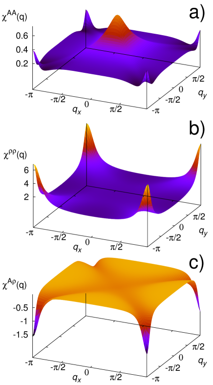
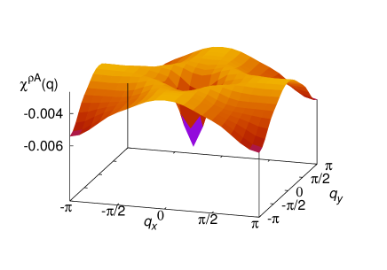
We start our considerations by a brief resume of the homogeneous case for which amplitude and density correlations have been analyzed in Ref. lara, and which are in agreement with our following finite cluster analysis. Fig. 1 shows the amplitude $\chi^{AA}({\bf q})$, density $\chi^{\rho\rho}({\bf q})$ and mixed $\chi^{A,\rho}({\bf q})$ correlation function for filling $n=0.875$ and $|U|/t=2$ without disorder.

For these parameters the maximum of the amplitude correlations is at ${\bf q}=0$ where it can be approximated as

$$\chi^{AA}({\bf q})\approx\frac{1}{m^{2}+cq^{2}}$$ (15)

with the mass $m$ and a parameter $c$ characterizing the dispersion of excitations. The quantity $\xi_{0}=\sqrt{c/m^{2}}$ can then be interpreted as a length scale for the decay of the amplitude correlations. On the other hand the density response is dominated by the contribution at ${\bf q}={\bf Q}\equiv(\pi,\pi)$ and around this wave-vector can be described by

$$\chi^{\rho\rho}({\bf q}\approx{\bf Q})\approx\frac{1}{m_{Q}^{2}+c_{Q}({\bf q}-{\bf Q})^{2}}\,.$$ (16)

In real space this corresponds to a staggered decay of the density correlations with length scale $\xi_{Q}=\sqrt{c_{Q}/m^{2}_{Q}}$.

The mixed susceptibility $\chi^{A,\rho}({\bf q})$ is negative (positive) for densities $n<1$ ($n>1$) since the anomalous correlations $\langle c_{i\downarrow}c_{i\uparrow}\rangle$ are negative with a maximum of their absolute value at half-filling. Therefore a positive fluctuation in density $\delta\rho$ for $n<1$ will lower (i.e. enhance the magnitude) the anomalous correlations.

Figure 2: (Color online) Distribution of the superconducting gap parameter $\Delta_{i}$ (displayed on a linear scale by circles) and superconducting currents (arrows) computed from Eq. (12) for constant vector potential $A_{x}$ and a specific disorder configuration. Parameters $|U|/t=5$, $V_{0}/t=2$. The dashed line (blue arrow) indicates the cut which is analyzed in Fig. 4.

For the present model, in the absence of disorder and at half-filling, there is an “accidental” symmetryyan90 which allows the superconducting order to be continuously rotated into the charge density wave (CDW) order at ${\bf q}={\bf Q}$ without energy change, promoting the charge density mode to a Goldstone mode. The enhancement of $\chi^{\rho\rho}({\bf Q})$ at $n=0.875$ is a remainder of this CDW instability at half-filling which is transfered to the amplitude correlations via the mixed susceptibility $\chi^{A,\rho}({\bf q})$ shown in the bottom panel of Fig. 1. Increasing $|U|/t$ enhances the CDW correlations so that at some point the ${\bf q}={\bf Q}$ amplitude correlations also dominate with respect to the ${\bf q}=0$ response. On the other hand the CDW correlations are suppressed in the dilute limit (not shown) so that upon reducing filling the maximum density response is first shifted away from ${\bf Q}$ along the Brillouin zone boundary and finally, below some concentration and depending on the value of $|U|/t$, the ${\bf q}=0$ response starts to dominate . A more detailed discussion on the filling dependence of the amplitude and density response in the clean case can be found in Ref. lara, .

III.2 Disordered system: Real space analysis

III.2.1 Mean-field solution

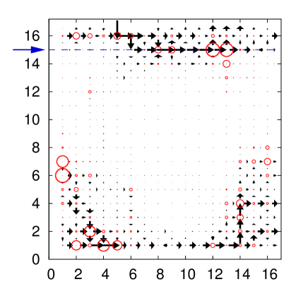
For sizeable disorder the density varies on the scale of the lattice constant and correlates with the strongly spatially fluctuating disorder potential. Further on, it has been shown in Refs. [ghosal98, ; ghosal01, ; dubi2007, ; sei12, ; ghosh13, ] that for strong disorder the system disaggregates into SC islands with sizeable SC gap $\Delta_{i}$ which are embedded in regions with $\Delta_{i}\approx 0$. Fig. 2 shows a map of the order parameter encoded on the size of the red circles showing the formation of the superconducting islands. This island structure leads to a very weak superfluid stiffness. Indeed, upon applying a transverse vector potential, as done in Ref. sei12, , the current flows through an optimum percolative path or “superconducting backbone” which determines the global stiffness. The latter not only depends on the volume fraction of the superconducting island, but also on the connectivity of these islands to the superconducting backbone. Thus one may have a moderate superconducting fraction and a very small global stiffness if the connectivity is poor. Fig. 2 shows an example of the superconducting backbone for current circulation. Notice that it does not necessarily involve all significantly superconducting sites. For example, sites $(1,7)$ and $(3,12)$ in Fig. 2, where $\Delta_{i}$ is large, are left out which therefore are examples for poorly connected islands. Whereas connected islands determine the superfluid stiffness the disconnected islands dominantly contribute to the subgap absortpion in the optical conductivity. cea14

Analyzing the mean-field solutions for several configurations of disorder we find that there is a strong tendency to form superconducting dimers. For example, for $V_{0}/t=2\sim 4$ we find that the average number of strongly superconducting neighbors of a strongly superconducting site is in the range $0.7\sim 0.8$. Here a strongly superconducting site is defined as a site with a local parameter $\Delta_{i}\geq 0.5\Delta_{max}$ where $\Delta_{max}$ is the largest value of $\Delta_{i}$ in the system (which is close to the maximal value $\Delta_{max}=|U|/2$) . Examples of dimers can be seen in Fig. 2 at sites $(1,6)-(1,7)$, $(12,15)-(13,15)$ and $(8,15)-(9,15)$. One also observes that dimers can act as seeds of more extended islands as in sites $(14,3)-(14,4)$.

Figure 3: (Color online) (a): Distribution of the superconducting gap parameter $\Delta_{i}$ (circles), the local density correlation function $\chi^{\rho\rho}_{ii}$ (squares), and nearest-neighbor density correlations $\chi^{\rho\rho}_{\langle ij\rangle}$ (bars on the bonds). (b): The distribution of the local $\chi^{AA}_{ii}$ (squares) and nearest-neighbor $\chi^{AA}_{\langle ij\rangle}$ (bars on the bonds) amplitude correlations together with the SC gap (circles). (c): Magnitude of local off-diagonal amplitude-density correlations $|\chi^{\rho A}_{ii}|$ (squares) together with the SC gap (circles). The disorder configuration and parameters are the same as in Fig. 2. The symbol size for the correlations is displayed on a logarithmic scale whereas the SC gap is plotted on a linear scale.

In previous work  ghosal98 ; ghosal01 it has been found that the preferable sites for the SC islands are those with the Hartree potential $H_{i}=-|U|\langle n_{i}\rangle+V_{i}$ being close to the chemical potential $\mu$, since this allows for strong particle-hole mixing. This would imply that the ’good’ SC sites are already encoded in the normal state since there exists a strong correlation between the local Hartree potentials in the SC and normal state. On the other hand the correlation between $H_{i}$ and the size of $\Delta_{i}$ weakens with increasing disorder, i.e. a small $|H_{i}-\mu|$ not necessarily correlates with a large $\Delta_{i}$ whereas a large $\Delta_{i}$ always implies a small $|H_{i}-\mu|$. A similar conclusion has been drawn in Ref. ghosh13, where the relation of order parameter variations and the shell effect has been investigated.

Figure 4: (Color online) Cut of the order parameter distribution (full line, circles) and local density susceptibility $\chi_{ii}^{\rho\rho}$ in the superconducting state (dashed line, squares) and in the normal state (dot dashed line, diamonds). The cut is done along the row with $y=15$ of Fig. 3b and is indicated by an arrow in Fig. 2.

III.2.2 Real space structure of responses

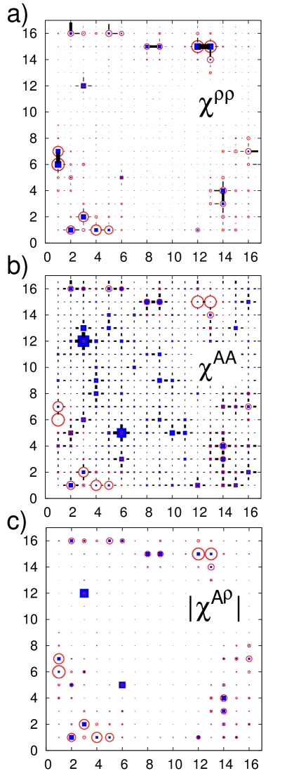
The largest contribution to the density and amplitude correlations comes from the diagonal elements $\chi_{ii}^{AA}$ and $\chi_{ii}^{\rho\rho}$ that are shown as a logarithmic map in Fig. 3a and b, respectively. Here the disorder realization is the same as in Fig. 2 and the local SC gap is shown with circles, whose size is proportional to the gap magnitude. Panel (a) shows also the nearest-neighbor density-density correlation $\chi^{\rho\rho}_{ij}$ encoded in the size of the bars on the bonds.

One finds that the strong superconducting sites coincide with sites which have a large charge density susceptibility. Also the dominant nearest neighbor density correlations $\chi^{\rho\rho}_{\langle ij\rangle}$ are attached to the SC islands and become particularly enhanced among the sites forming a SC dimer. We find that the bare local density correlations $\chi^{0,\rho\rho}_{ii}$ in the SC state show a similar structure (not shown) but with smaller absolute value ($\sim 1/20$).

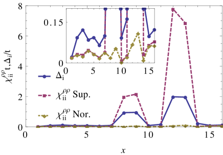
This rises the “chicken and egg” question if sites are favorable for superconductivity because they have a large susceptibility already in the normal state or if the large susceptibility is due to the local superconducting correlations. To answer this question we have computed the charge density susceptibility in the absence of superconductivity. Although there is a tendency for sites with charge density susceptibility larger than the average in the normal state to become superconducting, there is an enormous enhancement of the charge density susceptibility on the superconducting sites. This can be seen in the cut of the local susceptibilities and order parameter shown in Fig. 4. We see that on the superconducting sites the local susceptibility can be enhanced by two orders of magnitude. The inset shows a zoom of the intensity scale showing that the superconducting sites tend to have a charge density susceptibility larger than the average in the normal state but which does not explain the enhancement seen in the superconducting state. It also shows that on the sites with small order parameter the charge susceptibility remains the same in the superconducting and normal state. Clearly this behavior is due to the almost incompressible character of the phase without superconducting correlations which becomes instead highly compressible in the superconducting state. This physics is similar to that in the clean half-filled Hubbard model where a rotation between the two competing states, CDW and SC, essentially induces a transition from zero to very large compressibility $\kappa$.

Figure 5: (Color online) Plot of the points $(\Delta_{i},\chi_{ii}^{\rho\rho})$ (green) for the normal (left panels a, c) and SC (right panels b, d) system where $\Delta_{i}$ refers to the value in the SC state. The lines and errorbars have been obtained by collecting data in $10$ bins of $\Delta$. $|U|/t=2$, $V/t=1$ (upper panels a, b), $V/t=3$ (lower panels c, d).

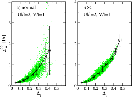
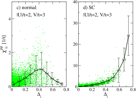
The correlation between SC gap and local charge density susceptibility is summarized in Fig. 5 which shows the distribution of $(\Delta_{i},\chi_{ii}^{\rho\rho})$ points from $200$ samples for the normal and SC state and two values of disorder at $|U|/t=2$. Here $\Delta_{i}$ always refers to the value in the SC state whereas $\chi_{ii}^{\rho\rho}$ is evaluated in both normal and SC state. In the normal state and for weak disorder $V/t=1$ one observes a positive correlation between the local $\chi_{ii}^{\rho\rho}$ and the gap $\Delta_{i}$ which would develop in the SC state. This correlation gets sharper in the SC state (panel b) but extends over the same range of $\chi_{ii}^{\rho\rho}$ values than in the normal state. In contrast, for larger disorder $V/t=3$ there is almost no correlation between local charge density susceptibility and SC gap in the normal state while this correlation is strongly enhanced in the SC state and pushed to values of $\chi_{ii}^{\rho\rho}$ which are one order of magnitude larger than in the normal state.

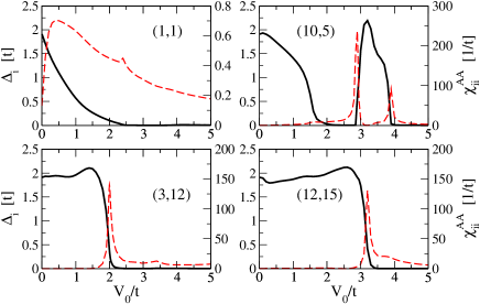
The behavior of the amplitude fluctuations is also very interesting. We find that local amplitude fluctuations are significantly enhanced when the SC gap displays strong variations as a function of disorder strength. This feature is exemplified in Fig. 6 which, for fixed disorder realization (the same as used in Fig. 2 and Fig. 3), shows the dependence of $\chi_{ii}^{AA}$ on $V_{0}$ for selected sites. One basically observes two kinds of behavior. First there are ’weak’ SC sites, as $(1,1)$ or $(10,5)$, whose order parameter immediately decreases with the onset of disorder. Besides there are ’strong’ SC sites, as $(3,12)$ or $(12,15)$ which initially resist disorder and where $\Delta_{i}$ can even get enhanced with respect to its $V_{0}=0$ value. The drop of $\Delta_{i}$ on the strong SC sites at a given $V_{0}/t$ is then accompanied by a peak in $\chi_{ii}^{AA}$ resembling the behavior close to a second order phase transition. However, the order parameter does not vanish on the disordered site of the transition but acquires a small finite value due to the proximity effect of other SC islands. For a given disorder strength only few sites are close to this regime and their number decreases with increasing $V_{0}/t$ due to the decrease of SC islands. There are also few sites, as $(10,5)$, where the SC order parameter reemerges at a large value of the disorder strength and stays finite over some range of $V_{0}$. In the appendix the behavior of $\Delta_{i}$ and $\chi_{ii}^{AA}$ for all sites of the sample is analyzed in more detail.

Figure 6: (Color online) Disorder dependence of the SC gap (solid, black) and of the local amplitude correlations (red, dashed) for selected sites of the disorder configuration used in Figs. 2,3. $|U|/t=5$.

The present real space analysis reveals that in the strongly disordered regime, density correlations are dominant on the SC islands whereas the amplitude correlations are large in the other part of the system, i.e. where the SC gap is almost completely suppressed by disorder. As shown in Fig. 3c there are only few sites with significant off-diagonal correlations $\chi_{ii}^{\rho,A}$. Besides on the ’marginal’ sites $(3,12)$ and $(6,5)$, which are at the transition $\Delta\to 0$, the mixing of amplitude and density correlations is only observed on some of the SC sites. Clearly this decoupling of amplitude and density correlations will be even more pronounced in the average momentum dependent correlations which will be analyzed in the next subsections.

III.3 Disordered system: Fourier space analysis

For a particular disorder configuration the Fourier transform of the correlation functions is given by

$$\chi({\bf q},{\bf q}^{\prime})=\frac{1}{N}\sum_{ij}e^{i\left({\bf q}{\bf R}_{i}-{\bf q}^{\prime}{\bf R}_{j}\right)}\chi_{ij}$$ (17)

where $N$ denotes the number of lattice sites. Clearly, if $\chi_{ij}$ only depends on the distance between lattice sites ${\bf R}_{i}-{\bf R}_{j}$ then $\chi({\bf q},{\bf q}^{\prime})$ is diagonal in momenta. In the following we perform averages of $\chi_{ij}$ over different disorder realizations up to $n_{d}=200$ for lattice sizes up to $24\times 24$. This procedure restores translational invariance in the correlation functions so that $\langle\chi({\bf q},{\bf q}^{\prime})\rangle_{conf.}\equiv\delta({\bf q},{\bf q}^{\prime})\chi({\bf q})$. In Figs. 8, 10 the errorbars in the compressibility and mass reflect the variance of $\chi({\bf q})$ at ${\bf q}=0$ and ${\bf q}={\bf Q}$, respectively. Although it increases with disorder and $|U|/t$ the mean-values exceed the variances for the ’worst’ cases by a factor $\sim 3$.

We fit the correlation function $\chi({\bf q})$, which is peaked at ${\bf q}={\bf Q}$, to the function

$$\chi({\bf q})=\lambda_{0}+\frac{\lambda_{3}}{1+2\lambda_{1}\gamma_{1}({\bf q}-{\bf Q})+2\lambda_{2}\gamma_{2}({\bf q}-{\bf Q})}$$ (18)

with

$$\gamma_{1}({\bf q}) = 2-\cos(q_{x})-\cos(q_{y})$$

$$\gamma_{2}({\bf q}) = 1-\cos(q_{x})\cos(q_{y})\,.$$

Although Eq. (18) yields a good account of the correlations over the whole Brillouine zone (BZ) the fit is restricted to an area of $\approx 5\%$ of the BZ around the peak at ${\bf Q}$ in order to extract the parameters in Eqs. (15,16). Expanding Eq. (18) around ${\bf Q}$ yields

$$m^{2} = \frac{1}{\lambda_{0}+\lambda_{3}}$$ (19)

$$c = \frac{\lambda_{1}+\lambda_{2}}{(\lambda_{0}+\lambda_{3})}$$ (20)

$$\xi^{2} = c/m^{2}=\lambda_{1}+\lambda_{2}\,.$$ (21)

In the following we analyze the momentum structure of the averaged density-, off-diagonal and amplitude correlations. The various fitting parameters will be distinguished by (a) the reference momentum in the expansion, i.e. ${\bf q}=0$ or ${\bf Q}\equiv(\pi,\pi)$, and (b) a superscript which indicates the correlation function. For example, $\xi_{0}^{A}$ will denote the correlation length for amplitude fluctuations derived from an expansion of $\chi^{AA}({\bf q})$ around ${\bf q}=0$.

Figure 7: (Color online) Average (number of samples $=200$) of Fourier transformed density correlations for parameter $|U|/t=2$, $V_{0}/t=3$.

III.3.1 Momentum structure of $\chi^{\rho\rho}({\bf q})$

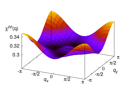
We start with the analysis of the momentum dependence of the averaged density correlation function which is shown in Fig. 7 for parameters $|U|/t=2$ and $V_{0}/t=3$. Disorder induces an overall suppression of the response as compared to the clean case in Fig. 1b. This is most pronounced for the CDW correlations at ${\bf q}={\bf Q}$ which for $V_{0}/t=3$ are reduced by a factor $1/20$ with respect to the clean case correlations. At ${\bf q}=0$ this reduction is only $1/2$ so that in Fig. 7 one observes a relative enhancement of the zone center correlations. For $|U|/t=2$ the crossover from dominant CDW to ${\bf q}=0$ correlations occurs at $V/t\approx 4$ whereas for larger values ($|U|/t=5$) $\chi^{\rho\rho}({\bf q})$ has a minimum at ${\bf q}=0$ up to the largest disorder investigated. Note that also for smaller filling disorder shifts the dominant correlations from incommensurate momenta in the clean case to ${\bf Q}=(\pi,\pi)$ so that the following analysis is representative for a wide doping range and disorder values.

Fig. 8 shows the parameters $(m_{Q}^{\rho})^{2}$ and $c_{Q}^{\rho}$ obtained from the fit to Eq. 18 with ${\bf Q}=(\pi,\pi)$ as a function of disorder together with the compressibility $\kappa=\chi^{\rho\rho}_{{\bf q}=0}$.

Figure 8: (Color online) Disorder dependence of the fit parameters $(m_{Q}^{\rho})^{2}$ (circles), $c_{Q}^{\rho}$ (squares), and $\xi_{Q}^{\rho}$ (diamonds) for the staggered density correlations extracted from Eqs. (18 - 21). The disorder dependence of the compressibility is shown by the triangles. The dashed-dotted line in panel d) indicates the correlation length in the normal state. In panel b) the normal state $\xi_{Q}^{\rho}$ is numerically identical to the result in the SC state.

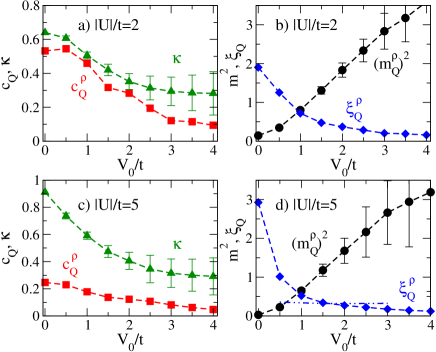
In the strong coupling limit (small $2t/|U|$) the clean case compressibility scales as $\kappa\approx|U|/8t^{2}$. lara The enhancement of $\kappa$ with $|U|/t$ can also be observed in Fig. 8 for $V_{0}/t=0$ although the parameters $|U|/t=2,5$ are rather in the intermediate coupling regime so that the agreement with the above estimate is only qualitative. Upon increasing $V_{0}/t$ there is first a decrease of $\kappa$, in agreement with the results of Refs. ghosal98, ; ghosal01, . At large disorder one observes a tendency of the average compressibility $\kappa$ to saturate to a value that is weakly dependent on $U$. Since in this regime the dominant contribution to $\kappa$ comes from the (real space) diagonal elements $\chi_{ii}^{\rho\rho}$ on the SC islands there exists an apparent inverse correlation between the number of SC islands (which decreases with $V_{0}/t$) and the local compressibility $\chi_{ii}^{\rho\rho}$ (which gets enhanced with increasing $V_{0}/t$).

We now turn to the analysis of the CDW correlation length in the disordered SC system. For weak disorder $V_{0}/t=0.5$ there is a strong difference in the density distribution obtained for the two values of $|U|/t=2,5$ which we have investigated. In fact, for $|U|/t=2$ we find that the difference in the density distribution between normal and SC state is small for each value of the disorder potential $V_{0}/t$. As a consequence the decrease of the CDW correlation length with $V_{0}/t$ (Fig. 8b) is the same in the normal and SC state within the numerical accuracy. On the other hand, for $|U|/t=5$ we find that already for $V_{0}/t=0.5$ sites in the normal state system are either almost empty or doubly occupied. As already discussed above, the SC state induces a redistribution of charge density which in this case leads to a significant rearrangement with a more homogeneous distribution between $n\approx 0.2$ and $n\approx 1.7$. As a consequence of this effectively less disordered SC state one observes in panel (d) of Fig. 8 an enhancement of the correlation length at $V_{0}/t=0.5$ from $\xi_{Q}^{\rho}\approx 0.3$ in the normal state to $\xi_{Q}^{\rho}\approx 1$ in the SC system.

The behavior of fit parameters in the SC system, as shown in Fig. 8, can then be qualitatively understood from the evolution toward the bimodal charge density distribution, where the low (high) density peak approaches $n_{L}=0$ ($n_{H}=2$) with increasing disorder. We also adopt the result from a strong coupling expansion of $\chi^{\rho\rho}({\bf q})$ for the homogeneous system lara ; note1 which for the mass parameter yields

$$m_{Q}^{2}=\frac{8t^{2}}{|U|}\frac{\delta^{2}}{1-\delta^{2}}$$ (22)

and $\delta=1-n$ denotes the doping measured from half-filling. Averaging Eq. 22 over the bimodal distribution. yields $\langle m_{Q}^{2}\rangle\sim(\delta n)^{2}/(1-(\delta n)^{2})$ with $\delta n=n_{H}-n_{L}$. The grow of $\delta n$ with $V_{0}/t$ then accounts for the increase of $m_{Q}^{2}$ with disorder as shown in Fig. 8.

In the strong-coupling clean case the parameter $c_{Q}$ is given by lara

$$c_{Q}=\frac{t^{2}}{|U|}\frac{1-2\delta^{2}}{1-\delta^{2}}=\frac{t^{2}}{|U|}-\frac{m_{Q}^{2}}{8}$$ (23)

and is thus expected to decrease with disorder proportional to the increase of $m_{Q}^{2}$. Within the numerical error this is in fact the behavior observed in Fig. 8 and also accounts for the decrease of the correlation length $\xi_{Q}$ with disorder.

III.3.2 Momentum structure of amplitude correlations

We proceed by analyzing the amplitude correlations $\chi^{AA}({\bf q})$ on top of the BdG solution whose momentum dependence is reported in Fig. 9 for $|U|/t=2$, $V_{0}/t=3$.

Figure 9: (Color online) Average (number of samples $=200$) of Fourier transformed amplitude correlations for parameter $|U|/t=2$, $V_{0}/t=3$.

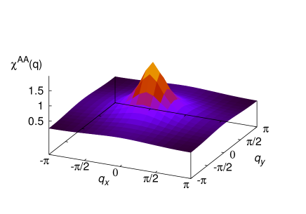
It turns out that disorder removes the enhancement of amplitude correlations at ${\bf Q}=(\pi,\pi)$, which were dominating in the clean case for this value of $|U|/t$. An interesting result is the concomitant enhancement of the ${\bf q}=0$ response by a factor of $\sim 5/2$ which therefore dominates the amplitude correlations for large disorder. As we have seen in the previous section, the density correlations are still peaked at ${\bf Q}=(\pi,\pi)$ for these parameters which indicates the decoupling of density and amplitude fluctuations with increasing disorder. Note that in contrast to the density correlations, the amplitude fluctuations in the normal state will always be unstable.

Figure 10: (Color online) Disorder dependence of the fit parameters $(m0^{A})^{2}$ (circles), $c_{0}^{A}$ (squares) and $\xi_{0}^{A}=\sqrt{c_{0}^{A}/(m_{0}^{A})^{2}}$ (diamonds, right inset) as extracted from Eqs. (18 - 21) for $|U|/t=2$ (a) and $|U|/t=5$ (b). The left inset reports the average superconducing gap (circles) and average spectral gap (squares). The right insets also show the gap autocorrelation length $\lambda_{ac}$ (circles) computed from Eqs. (24,25).

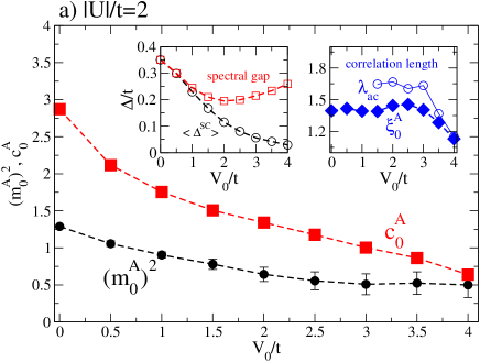
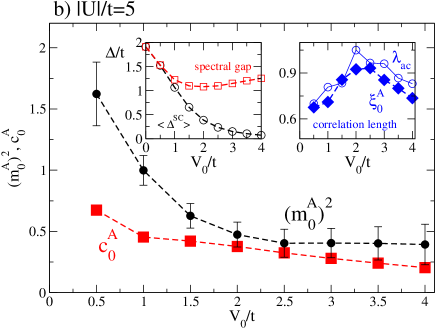
The latter are again characterized by the mass $(m_{0}^{A})\texttwosuperior$ and $c_{0}^{A}$ parameter obtained from the fit of $\chi^{AA}({\bf q})$ to Eq. 18 around ${\bf q}=(0,0)$. Fig. 10 reports the fit parameters as a function of disorder, again for values of the onsite attraction $|U|/t=2$ and $|U|/t=5$. Note that for the larger interaction $|U|/t=5$ and small disorder the correlations show the dominant peak at ${\bf Q}=(\pi,\pi)$ for which reason the fit parameters are only reported for $V_{0}/t\geq 0.5$.

The aforementioned enhancement of the ${\bf q}=(0,0)$ amplitude correlations with $V_{0}/t$ now results in the decrease of the mass $m_{0}^{A}$ with disorder with tendency to saturate at large $V_{0}/t\gtrsim 2$. Also the parameter $c$ decreases with the disorder strength so that the resulting correlation length $\xi_{0}^{A}=c_{0}^{A}/(m_{0}^{A})^{2}$ (right insets to Fig. 10) crucially depends on the relative change of $c_{0}^{A}$ and $(m_{0}^{A})^{2}$ with $V_{0}/t$.

For $|U|/t=2$ the correlation length is almost constant up to $V_{0}/t=2.5$ and then starts to decrease with disorder. For larger $|U|/t$ one even observes an enhancement for small $V_{0}/t$ so that $\xi_{0}^{A}$ acquires a maximum around $V_{0}/t=2.5$. We note that this is not an effect of competing CDW order since the same result is observed in the low-density regime where such correlations are absent.

In the limit of small $V_{0}/t$ one can adopt the usual expression for the correlation length in dirty superconductors given by $\xi_{0}=\sqrt{\xi_{BCS}l}$ with the mean free path $l$ and the correlation length of the clean system $\xi_{BCS}\sim v_{F}/\Delta^{SC}$. The behavior of $\xi_{0}(V_{0})$ therefore crucially depends on the depletion of the density of states, which lowers the superconducting $\Delta^{SC}$ gap, and the reduction of the mean free path $l$ with disorder. As noted in Ref. ghosal98, ; ghosal01, the situation in the strongly disordered system is more interesting since one has to distinguish between the average superconducting order parameter $\langle\Delta^{SC}\rangle$ and the spectral gap. As shown in the left insets to Fig. 10 $\langle\Delta^{SC}\rangle$ continuously decreases with disorder due to the increase of the ’non-SC’ area. On the other hand the spectral gap first shrinks with disorder due to the depletion of the density of states but grows again for strong disorder, signaling the formation of local boson pairs that get progressively localised as the SIT is approached. One can then argue that at strong disorder the BCS correlation length tends to scale as the inverse of the spectral gap, that acts as a cut-off to the increase of $\xi_{0}$ associated to the suppression of the SC order parameter. Alternatively one can relate the disorder dependence of the correlation length to the behavior of the nearest-neighbor amplitude correlations as shown in the appendix.

Figure 11: (Color online) Average of Fourier transformed off-diagonal correlations $\chi^{A\rho}({\bf q})$ for $V_{0}/t=2.0$ and $|U|/t=2$.

Recentlykaml13 the spatial dependence of the STM spectra in strongly disordered NbN films has been analysed in terms of the autocorrelation function for the order parameter, i.e.

$$\langle C({\bf R})\rangle=\frac{1}{N}\langle\sum_{i}\left(\Delta_{i}-\langle\Delta\rangle\right)\left(\Delta_{i+{\bf R}}-\langle\Delta\rangle\right)\rangle.$$ (24)

By performing an average over several disorder configurations we can extract the corresponding correlation length $\lambda_{ac}$ from a fit to the function

$$F({\bf R})=a_{0}+a_{1}\mbox{e}^{-R/\lambda_{ac}\left(1+a_{2}\sin^{2}(2\phi)+a_{3}\sin^{2}(4\phi)\right)}\,.$$ (25)

Here $\phi$ is the polar angle related to ${\bf R}$ which incorporates anisotropies in the correlations and we restrict the fit to $|{\bf R}|>2$ in order to isolate the long-distance behavior. The resulting length $\lambda_{ac}$ as a function of disorder is shown by circles in the right inset to Fig. 10 and it is close to the correlation length $\xi_{0}^{A}$ extracted from the amplitude correlations. For $V_{0}\rightarrow 0$ one can apply linear response theory on the disorder and show that the two lengths coincide. In the strongly disordered regime the situation is more complex. We find numerically that both lengths are close to each other. Notice that for $|U|/t=5$ we observe that both $\lambda_{ac}$ and $\xi_{0}^{A}$ increase in the regime where the separation between the order parameter and the spectral gap starts to develop, while they collapse in the regime where the spectral gap tends to increase again. In Monte Carlo simulationsboua11 the latter regime corresponds to the SIT, not captured by the present Bogoliubov-de-Gennes approach. This same tendency is observed in the experimental estimate of $\lambda_{ac}$ given in Ref. kaml13, , done for samples in the so-called ”pseudogap” region of the phase diagram, where the spectral gap is much larger than $T_{c}$.

III.3.3 Momentum structure of off-diagonal correlations

Off-diagonal correlations $\chi^{A\rho}({\bf q})$ mix the density and amplitude sector and are shown in Fig. 1 for the clean case and in Fig. 11 for the disordered system.

Upon coupling an external field in the density sector $H_{1}=\sum_{\bf q}\lambda_{\bf q}\rho_{\bf-q}$ the correlation function $\chi^{A\rho}({\bf q})$ yields the corresponding response for the gap amplitude. In particular, for ${\bf q}=0$ a spatially constant (and positive) $\lambda_{{\bf q}=0}$ induces an effective reduction of the chemical potential. Consider now the clean case where for the attractive Hubbard model with nearest-neighbor hopping the gap amplitude as a function of density has a maximum at half-filling and continuously decreases towards $n=0$ and $n=2$. Therefore off-diagonal correlations are negative for $n<1$ (where a positive $\lambda$ shifts the effective chemical potential away from half-filling) in agreement with Fig. 1 and positive for $n>1$. Similar arguments can be made for finite momenta. In particular, the strong enhancement of $|\chi^{A\rho}({\bf q})|$ at ${\bf q}={\bf Q}_{CDW}$ observed in Fig. 1 is due to the strong competition between CDW and SC correlations close to half-filling.

In the doped system Fig. 11 reveals a strong suppression for the off-diagonal correlations due to the spatial separation of density- and amplitude fluctuations as demonstrated in Sec. III.2. Naturally this is again most pronounced for the CDW momentum due to the removal of particle-hole symmetry by disorder. It is worth noting that in the dynamic limit (${\bf q}=0,\omega$ finite) the off-diagonal correlations show instead the opposite behavior. More specifically, as it has been recently discussed in Ref. [cea_cm15, ], the coupling between the amplitude and density/phase correlation at finite frequency is strongly enhanced by disorder, leading to a strong mixing between the amplitude and phase spectral functions at zero momentum.

IV Current correlations

To conclude our analysis of the SC correlations we shall discuss now the change in the current-current correlation function induced upon entering the superconducting state. In particular we want to explore the consequences of the percolative current formation (cf. Fig. 2) on the behaviour of the current correlation function $\chi^{jj}$ entering the definition (12) of the superfluid stiffness.

In order to obtain the intrinsic superconducting response, we have to subtract the contribution which is already present in the normal state (at finite momenta), and which can be either diamagnetic or paramagnetic depending on the filling of the system.

This is illustrated by the dashed line marked with diamonds in Fig. 12 for the homogeneous non-superconducting system. Clearly, the current response of Eq. (14), $D_{q_{y}}=-\langle T_{x}\rangle+\langle\chi^{jj}({q_{y}})\rangle$ vanishes at $q_{y}=0$ (i.e. the SC stiffness) when the system is in the normal state, however, it becomes non-zero for finite momenta.

Figure 12: (Color online) Transverse current response $D_{q_{y}}=-\langle T_{x}\rangle+\langle\chi^{jj}({q_{y}})\rangle$ for the non-SC (blue dashed, diamonds) and the sc homogeneous system at $|U|/t=5$ (red dashed, triangles). The normal state response ($\Delta_{sc}=0$) is independent of $|U|/t$. The solid lines report the difference $\Delta D_{s}(q_{y})$ between $D_{q_{y}}$ for the sc- and normal system for $|U|/t=5$ (squares) and $|U|/t=2$ (circles). Filling $n=0.325$ (a) and $n=0.875$ (b).

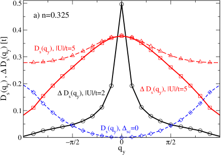
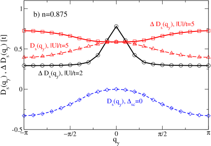
In particular at low density (cf. Fig. 12a) one recovers the finite-q diamagnetic response ($D_{q_{y}}>0$) related to Landau diamagnetism in agreement with the transverse current response of a Fermi liquid. pinesbook In contrast, larger filling (cf. Fig. 12b) supports a finite-q paramagnetic current response which would even diverge at ${\bf q}=(\pi,\pi)$ for $n=1$ (not shown). This feature is the starting point for the exploration of circulating current phases as possible candidates for the pseudogap in cuprate superconductors. schulz89

As shown by the triangle symbols in Fig. 12 a finite SC gap shifts up the curves in order to yield a diamagnetic $D_{q_{y}}$ independently on doping. In order to extract what is due to superconductivity we take the difference with respect to the normal state response $D^{normal}_{q_{y}}$ and the corresponding curves are shown by square symbols ($|U|/t=5$) and circles ($|U|/t=2$) in Fig. 12 for $n=0.325$ and $n=0.875$, respectively. In the weak coupling limit the difference $\Delta D_{s}(q_{y})=D^{SC}_{q_{y}}-D^{normal}_{q_{y}}$ is always strongly peaked at $q_{y}=0$ and the underlying normal state response does not influence the curvature of the peak which determines the SC coherence length. On the other hand, it turns out that for large filling and strong coupling (cf. squares in Fig. 12) $\Delta D_{s}(q_{y})$ can even acquire a maximum at the zone boundary. Thus in this limit the SC diamagnetic response is largest on short length scales and corresponds to an oscillatory decay of the SC induced current correlations in real space.

Fig. 13 shows the transverse current response $\Delta D_{s}(q_{y})$ for various disorder strength and interaction $|U|/t=2$ with the normal state result substracted. The latter has obtained for the same disorder configurations and by setting $\Delta^{SC}_{i}=0$.

Figure 13: (Color online) Main panel: Transverse current correlations $\Delta D_{s}(q_{y})$ measured with respect to the normal system for $|U|/t=2$, $n=0.875$, and various disorder strengths. Upper left inset: Correlation length extracted from Eq. (26). Upper right inset: Superfluid stiffness.

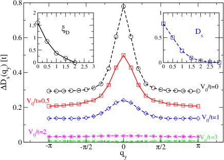
We parametrize the long-wavelength structure as

$$\Delta D_{s}(q_{y})=D_{s}\left[1-(\xi_{D}q_{y})^{2}\right]$$ (26)

which defines a SC coherence length related to the diamagnetic response and allows us to extract the stiffness $D_{s}$ as a function of disorder. Both quantities are shown in the insets to Fig. 13.

As discussed previously sei12 (see also Sec. III.2.1) $D_{s}$ gets rapidly suppressed with disorder but since the BdG approach does not capture the SC-insulator transition it does not vanish even for large $V_{0}/t$. Also the coherence length (cf. left inset to Fig. 13) is strongly suppressed by disorder. Above $V_{0}/t\approx 2$, $\Delta D(q_{y})$ is essentially independent on the transverse momentum $q_{y}$ and $\xi_{D}\approx 0$ within the numerical accuracy.

However, due to the average over disorder configurations the above analysis does not capture the long-range current correlations which exist along the percolative path (cf. Sec. III.2) and which we will analyze separately in the following.

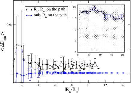
First we identify the superconducting backbone. The criterion to decide which sites belong to the percolative path is chosen as follows: For the vector potential ${\bf A}$ along the $x$ direction, we determine the maximum current through a bond $j_{x}^{max}$ in the system and select all sites which have currents larger than $\alpha j_{x}^{max}$. We find that usually a value of $\alpha=1/3$ is appropriate in order to selecting the sites which are visited by the path. An example is shown in the inset to Fig. 14 where the squares indicate sites with $j_{x}(R_{n})>j_{x}^{max}/3$. Clearly, there are sites (e.g. in the upper right corner) which are traversed by a minor current but are left out by the ’$\alpha=1/3$’ criterion. Reducing further the value of $\alpha$ would also include these sites, however, we note that the following results do not depend sensitively on the value of $\alpha$. The effect of a larger (smaller) $\alpha$ is to add sites with larger (smaller) current to the path which concomitantly slightly increases (decreases) the long-distance correlations which are calculated below.

Figure 14: (Color online) Main panel: $\langle\Delta D_{nm}\rangle$ for both sites (black) and only one $R_{n}$ (blue) on the percolative path shown in the inset. The squares indicate sites $R_{n}$ with $j_{x}(R_{n})>j_{x}^{max}/3$. $|U|/t=2$, $n=0.875$, $V/t=3$.

We proceed by evaluating the non-local stiffness $D_{n,m}$ between sites $R_{n}$ and $R_{m}$

$$D^{xx}_{nm}=\left[-\delta_{n,m}t_{x}(n)-\chi_{nm}(j^{x}_{n},j^{x}_{m})\right]$$ (27)

and compute the difference between sc and normal state $\Delta D_{nm}=D^{sc}_{nm}-D^{nl}_{nm}$. Two cases are considered: (a) both sites $R_{n}$ and $R_{m}$ belong to the percolative path and (b) only one of the sites $R_{n}$, $R_{m}$ is on the path. The result for $D_{nm}$ in both cases is shown in Fig. 14 for the particular percolative path displayed in the inset. The ’errorbars’ indicate the variance due to the fact that different sites $R_{n}$ and $R_{m}$ have the same distance $|R_{n}-R_{m}|$ but different values for $D_{nm}$.

As can be seen the current correlations rapidly decay away from the percolative path and are practically ’zero’ for $|R_{n}-R_{m}|>3$. On the other hand correlations on the path stay finite up to the largest distances available in the system.

Figure 15: (Color online) Current correlations $\langle\Delta D_{nm}\rangle$ averaged over 200 samples for disorder strength $V/t=3$ and $n=0.875$. Full symbols: $|U|/t=2$; Open symbols: $|U|/t=5$.

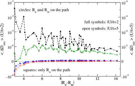
Finally, Fig. 15 shows the on- and off-path current correlations averaged over $200$ disorder configurations for $|U|/t=2$ and $|U|/t=5$, respectively. As for the specific sample shown in Fig. 14 the off-path correlations get rapidly suppressed while on-path correlations stay finite up to large $|R_{n}-R_{m}|$. Upon comparing the on-path correlations between the two $|U|/t$-values one finds, besides a reduction by a factor of $\approx 10$, that the decay of $\Delta D_{nm}$ with distance for $|U|/t=5$ is significantly smaller than for $|U|/t=2$ while still staying finite for the largest possible separation in the system ($\approx\sqrt{2}\times 10$ for a $20\times 20$ lattice when the percolative path is along the diagonal).

The persistance of the current correlations along the percolative path resembles closely the expected behavior for a one-dimensional chain, where it simply follows from the current conservation. This can be easily seen at $\omega=0$ by using the following classical phase-only action:

$$S=\frac{1}{2}\sum_{i}J_{i}(\delta\Phi_{i})^{2}$$ (28)

where $J_{i}$ are the local (random) stiffnesses (in units of the temperature $T$) and $\delta\Phi_{i}$ represents the local phase gradient $\delta\Phi_{i}\equiv(\theta_{i+1}-\theta_{i})$, $\theta_{i}$ being the local SC phase. Eq. (28) can be obtained for example by expanding at Gaussian level a classical $XY$ model with random couplings $J_{i}$, that is the prototype model for the phase degrees of freedom of a superconductor. Eq. (28) is also obtainedcea14 by mappingma_prb85 at large $U$ the disordered Hubbard model into the pseudospin model. In this mapping the superconductivity corresponds to a spontaneous in-plane magnetization, i.e. to the usual $XY$ model with a coupling $J\sim t^{2}/U$, and disorder maps into a random out-of-plane field, that leads in turn to the disorder in the local couplings $J_{i}$ after a Holstein-Primakoff expansion around the mean-field solution. cea14

The local current $I_{i}$ for the model (28) can be written, after minimal coupling substitution $\delta\Phi_{i}\to\delta\Phi_{i}-2A_{i}$ in Eq. (28) as:

$$I_{i}=2J_{i}(\delta\Phi_{i}-2A_{i})\,.$$ (29)

In the one-dimensional case the current conservation implies that $I_{i}$ is independent on the site index, i.e. $(\delta\Phi_{i}-2A_{i})=c/2J_{i}$, where $c$ is a constant. By summing over the site index and using the boundary condition $\sum_{i}\delta\Phi_{i}=0$ one then gets $c=-4(\sum_{i}A_{i})/\sum_{i}(1/J_{i})$. Since the superfluid stiffness is defines as usual (see Eq. (14)) as $D_{s}=-I(q=0)/A(q=0)$ one also deduces that

$$D_{s}=4\left(\frac{1}{N}\sum_{i}\frac{1}{J_{i}}\right)^{-1}$$ (30)

so that $I_{i}=c=-(1/N)\sum_{j}D_{s}A_{j}$. By comparing this with Eq. (27) above we then recover that $D_{ij}=D_{s}/N$ for all pairs of sites $i,j$ along the chain. It is interesting to note that this result also implies that the paramagnetic contribution to the current must cancel out the local diamagnetic term $4J_{i}$ of Eq. (29). This can be seen by computing explicitly the average current value from Eq. (29) in linear response theory, in analogy with the expression (27) introduced above:

$$\langle I_{i}\rangle=-4\sum_{j}J_{i}(\delta_{ij}-X_{ij}J_{j})A_{j}\equiv-\sum_{j}D_{ij}A_{j}$$ (31)

where $X_{ij}=\langle\delta\Phi_{i}\delta\Phi_{j}\rangle$ is easily determined from Eq. (28) as:

$$\langle\delta\Phi_{i}\delta\Phi_{j}\rangle=$$

$$\frac{\int d\lambda{\cal D}\delta\Phi\exp\left[-\frac{1}{2}\sum_{k}J_{k}(\delta\Phi_{k})^{2}+i\lambda\sum_{k}\delta\Phi_{k}\right]\delta\Phi_{i}\delta\Phi_{j}}{\int d\lambda{\cal D}\delta\Phi\exp\left[-\frac{1}{2}\sum_{k}J_{k}(\delta\Phi_{k})^{2}+i\lambda\sum_{k}\delta\Phi_{k}\right]}$$

where the $\lambda$ integration accounts for the periodicity constraint. By making the change of variables $\delta\Phi_{k}\to\delta\Phi_{k}-i\lambda/J_{k}$ one immediately sees that

$$X_{ij}=\frac{\delta_{ij}}{J_{i}}-\frac{D_{s}}{NJ_{i}J_{j}}$$ (33)

that inserted into Eq. (31) gives $D_{ij}\equiv D_{s}/N$, as anticipated before. We note also that the independence of $D_{ij}$ in Eq. (31) on both site indexes can be also derived as a consequence of charge conservation and gauge invariance in one dimension. Indeed the independence of $D_{ij}$ on the site index $i$ is a consequence of a constant current $I_{i}$ on each site, while the independence of $D_{ij}$ on the second index $j$ is a consequence of the fact that at $\omega=0$ only to the $q=0$ component of the gauge field $A$ leads to a finite response.

Going back to our 2D system, we clearly see in Fig. 15 that for a fixed disorder strength the percolative path becomes more ’1D’-like with increasing $|U|/t$, which accounts for the crossover to a more constant $\Delta D_{nm}$ for $|U|/t=5$. Indeed, a larger $|U|/t$ corresponds to a smaller $J$ in the mapping into the $XY$-like bosonic model, with an enhanced influence of disorder and with smaller effective local stiffnesses ${J_{i}}$. This in turn is in agreement with the strong reduction of $\Delta D_{nm}$ from $|U|/t=2$ to $|U|/t=5$, as shown in Fig. 15.

V Discussion and Conclusions

As we discussed in the introduction, it has been now established in several theoretical models that when the SIT is approached a granular SC state emerges, with SC puddles embedded in a non-SC background. Thanks to the enormous progresses made in the experimental techniques able to probe the systems in real space, it has been also established that such an emergent granularity is observed in disordered films of conventional superconductors, like e.g. NbN, InO_x and TiN. sac08 ; sac10 ; mondal11 ; chand12 ; kaml13 ; noat13 It is then crucial to assess how this inhomogeneous SC state affects the behavior of the amplitude, density and current correlations, in order to interpret the results of the various experimental probes.

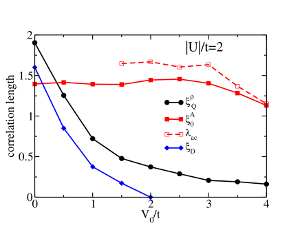
In the present manuscript we analyzed this issue within the fermionic Hubbard model with on-site disorder. We presented a detailed study of the correlation functions both in real space, for a specific disorder configuration, and in momentum space, after the average over several disorder configurations. The momentum-space analysis allows us to extract the correlation length of each physical quantity in close analogy with the usual approach for homogeneous systems. As a first result, one then sees that while in the homogeneous case at low temperature amplitude and current correlation lengths coincide up to a numerical factorlara , in the presence of strong disorder this is no more true as can be seen in the summarizing figure 16. By means of a simultaneous analysis of the real-space correlations we can then disentangle how the properties of the fragmented SC ground state influence the various correlation lengths. As we discussed in the manuscript, these two approaches give complementary informations, that we will summarize below. In this respect, even though our results are based on a RPA approximation, they have the advantage to allow for larger system sizes than Monte Carlo simulations, as e.g. those reported in Ref. scal99, . The use of large clusters is in turn crucial to trace back the behavior of different response functions to the inhomogeneous structure of the ground state and to perform a momentum-space analysis.

Figure 16: (Color online) Summary of results for the various correlation lengths as a function of disorder for $|U|/t=2$ and $n=0.875$. At very small disorder the autocorrelation length $\lambda_{ac}$ cannot be properly defined since the approximated formula (25) does not reproduce accurately the data, see also $C(R)$ in Fig. 17 below.

Amplitude and density correlations.

We find that in general the strength of the amplitude response $\sim 1/(m_{0}^{A})^{2}$ increases with disorder while the charge response $\sim 1/(m_{Q}^{\rho})^{2}$ gets suppressed by disorder (cf. Figs. 8 and 10). This is similar to a previous Monte Carlo studyscal99 which found that superconducting correlations are much more robust to disorder than charge correlations. Here, due to the larger system size, we could explore in detail the origin of this behavior.

The suppression of the charge response is easily understood by the tendency of disorder to localize the pairs and render the system incompressible almost everywhere except in the superconducting islands. The increase of the superconducting response is more subtle. For strong disorder the region in between the islands contains “marginal” sites where the order parameter is small but very susceptible to become large by small variations of the disorder [see Fig. 3(b) and Fig. 6 for site (3,12)] yielding a large overall pair susceptibility and resembling the behavior close to a second order phase transition. The decoupling of density and amplitude correlations in real space is reflected in the momentum-space structure of the susceptibilities. Thus, while in the homogeneous caselara the maximum or $\chi_{\rho\rho}({\bf q})$ at the CDW vector ${\bf Q}=(\pi,\pi)$ leads to an enhancement of the amplitude correlations $\chi_{AA}({\bf q})$ at the same wavevector (see Fig. 1), in the disordered case this effect disappears (Fig. 9).

The resulting amplitude correlation length $\xi^{A}_{0}$, shown in Figs. 10, 16 has an interesting disorder dependence. Indeed, it stays constant or it is even enhanced at intermediate disorder levels, before then being ultimately suppressed as the SIT is approached. In the latter regime we argued that the decay of the correlation length is ruled by the behavior of the spectral gap, which increases as pairs become localized with disorder.

Figure 17: Comparison between the experimental estimate (left panel) of the autocorrelation function, defined in Eq. (24), and the numerical computations (right panel). The experiments data are taken from Ref. [kaml13, ] and refer to three NbN films at different disorder level (labeled by the different critical temperatures $T_{c}$). The theoretical data are obtained for $|U|/t=2$, $n=0.875$, and disorder values $V_{0}/t=0.5$ (solid) and $V_{0}/t=3.$ (dashed). Considering that the typical size of the SC islands in these NbN films range between 20-40 nm, and it is one-two lattice spacings in our simulations, the length scales in the experiments and simulations are approximately comparable.

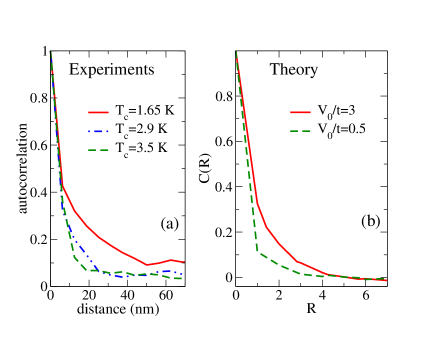
In Figs. 10, we also compared $\xi_{0}^{A}$ with the autocorrelation length $\lambda_{ac}$, that can be directly extracted experimentally from the STM maps of the SC ground state. This has recently been done for disordered NbN films kaml13 and we show for convenience the corresponding data in Fig. 17a. In this work the SC islands are identified by the regions with a large SC coherence-peak height, that is usually takenboua11 ; lem13 to be a measure of the local order parameter $\Delta_{i}$, i.e. the local gap solution in the BdG equations. By analyzing the spatial correlations between good SC sites the authors of Ref. [kaml13, ] found that the autocorrelation length $\lambda_{ac}$ becomes larger as disorder is increased. This is shown in Fig. 17a where we report the experimental data for the autocorrelation function $C(R)$ defined in Eq.  (24) above. A similar trend can be observed also in our simulations, see Fig. 17b, where $C(R)$ shows first a rapid suppression over a length scale of the order of the SC island, followed by a long-tail decay that can be eventually fitted with the approximated formula (25) in order to extract $\lambda_{ac}$. Since this tail can be thought as the response of the system to the fluctuations that created the island we expect that $\lambda_{ac}$ is close to $\xi_{0}^{A}$, as indeed we find numerically, see Fig. 10 and Fig. 16.

In contrast to the autocorrelation length, a direct estimate of the amplitude correlation length $\xi_{0}^{A}$ from the experiments is not so straightforward. Indeed, while within a Ginzburg-Landau approach, where a single length scale exists, $\xi_{0}$ can be estimated from the upper critical field at $T=0$ as $H_{C2}=\Phi_{0}/(2\pi\xi_{0}^{2})$, at strong disorder this connection is not obvious. In particular when the superfluid stiffness $D_{s}$ is the lowest energy scale in the problem one would expect that $T_{c}\propto D_{s}$, so that also the upper critical field will scale with $D_{s}$, as suggested for example by a recent analysis of the microwave conductivity at finite magnetic field in disordered InO_x. armitage_prl13 In this sense, even though at intermediate disorder the decrease of $H_{c2}$ measured experimentally pratap11 can be interpreted as an increase of $\xi_{0}$ due to the weakening of the SC order parameter, as the SIT is approached one should not attribute the vanishing of $H_{c2}\propto T_{c}$ to a divergence of $\xi_{0}^{A}$ discussed above.

Current correlations The behavior of the current correlations is also strongly influenced by the formation of a fragmented SC state. Indeed, as already noticed before,sei12 the superfluid response is mainly determined by a few percolative paths that connect the good SC regions. As a consequence, the decay of the current correlations depends on the position of the initial and final sites with respect to this SC ’backbone’. If both sites belong to a percolative path the current correlations are long-ranged (essentially constant, see Fig. 14), in agreement with what one expects for a truly one-dimensional system, like e.g. the one-dimensional $XY$-model. On the other hand, this long-range behavior is easily missed when the transverse current correlations are extracted from the response in momentum space after average over several disorder configuration. Indeed, the current-current correlation length $\xi_{D}$ is rapidly suppressed (cf. inset to Fig. 13 and Fig. 16a), in analogy with the overall superfluid response. This behavior has to be contrasted to the one of the amplitude correlation length $\xi_{0}^{A}$, that is strongly suppressed only at the SIT. On the other hand, the persistence of current correlation along the percolative paths suggests that the existence of the SC backbone can be deduced in principle by the measurements of the space-dependent current susceptibilities, without having to evaluate explicitly the current pattern at finite applied field. The experimental study of these issues is of course challenging, but it should be accomplishable with four-point atomic force microscopy when the electrode spacing reaches the nanometer separation. Its observation would certainly contribute significantly to our understanding of the basic mechanisms leading to the formation of the inhomogeneous SC state as the SIT is approached in real systems.

Figure 18: (Color online) Top panel: disorder dependence of the SC gap value for the same disorder configuration used in Figs. 2, 3. The site index for the $16\times 16$ lattice is obtained from $i_{x}+16(i_{y}-1)$. Lower panel: disorder dependence of the local amplitude correlations $\chi^{AA}_{ii}$ normalized to their maximum value at each site. $|U|/t=5$, $n=0.875$.

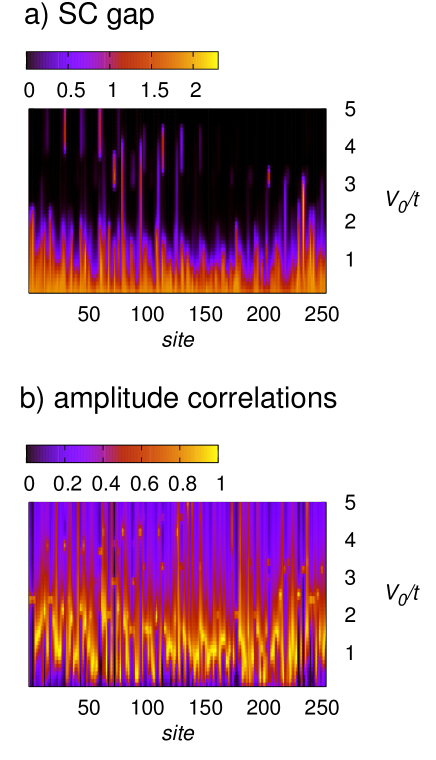
Appendix A Disorder dependence of local SC gap and local correlations

Fig. 19 reports the disorder dependence of the SC gap value and local amplitude correlations on each site for the same disorder configuration and parameters used in Figs. 2, 3. Note that the amplitude correlations are normalized to their maximum value at each site. Clearly, the SC order parameter on the majority of sites drops to a small value around $V_{0}/t\approx 2$ but there are also singular sites where $\Delta_{i}$ extends up to $V_{0}/t\approx 4$ or where $\Delta_{i}$ reemerges at large disorder values.

In the clean system the onset of a finite SC gap below $T_{c}$ is accompanied by a divergence in the amplitude correlations, both the local and non-local ones. The pronounced enhancement of the amplitude correlations around $V_{0}/t\approx 2$ in Fig. 18b suggests a similar feature as a function of disorder with the difference that $\Delta_{i}$ does not vanish but becomes small beyond some value of $V_{0}$. To analyze this feature in more detail we plot in Fig. 19 the probability density $P(\Delta<\epsilon)$ as a function of the disorder strength $V_{0}$. Here $P(\Delta<\epsilon)dV_{0}$ is the probability that the order parameter of a given site will fall below the threshold $\epsilon$ for the first time when the disorder is increased from $V_{0}$ to $V_{0}+dV_{0}$. Also shown are the probability distributions for the maximum in the local [$P(\chi^{AA}_{ii}=max)$] and nearest neighbor [$P(\chi^{AA}_{\langle ij\rangle}=max)$] amplitude correlations where, for example, $P(\chi^{AA}_{ii}=max)dV_{0}$ is the probability that $\chi^{AA}_{ii}$ for a given site $i$, attains its maximum value as a function of disorder in the interval $V_{0}$, $V_{0}+dV_{0}$. Clearly, for $|U|/t=5$ (right panel of Fig. 19) $P(\Delta<0.01t)$ has a pronounced peak around $V_{0}/t\approx 2\dots 2.5$ and one finds that for about $50\%$ of all sites $\Delta_{i}<0.01t$ between $1.5<V_{0}/t<2.5$. Concomitantly also the probability distributions for the local and non-local amplitude correlations are peaked at a somewhat lower value of $V_{0}/t\approx 1.5$. For smaller $|U|/t=2$ these distributions are broader and in particular the nearest-neighbor amplitude correlations are no longer characterized by a significant enhancement.

Figure 19: (Color online) Black (full) steps: Probability distribution $P(\Delta<\epsilon)$ that the order parameter of a given site will fall below the threshold $\epsilon$ for the first time, upon increasing the disorder with $\epsilon=0.01t$ ; Red dashed step: Probability distribution $P(\chi^{AA}_{ii}=max)$ that the local amplitude correlation of a given site will attain its maximum value as a function of disorder strength. Blue thin step: Probability distribution $P(\chi^{AA}_{\langle ij\rangle}=max)$ that the nearest-neighbor amplitude correlations of a given bond will attain its maximum value as a function of disorder strength. Left panel: $|U|/t=2$, Right panel: $|U|/t=5$.

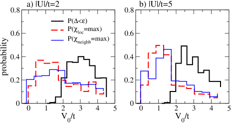
This finding offers an alternative perspective for understanding the disorder dependence of the amplitude correlation length $\xi_{0}$ shown in Fig. 10. Since $\xi_{0}$ is of the order of one lattice spacing the nearest-neighbor correlations yield the dominant contribution to the correlation length which accounts for the enhancement around $V_{0}/t=2$. On the other hand, the distributions as a function of $V_{0}/t$ are significantly broader for $|U|/t=2$ (cf. Fig. 19a) which agrees with the behavior of $\xi_{0}$ shown in Fig. 10a.

References

- (1) P. W. Anderson, J. Phys. Chem. Solids 11, 26 (1959).
- (2) D. B. Haviland, Y. Liu, and A. M. Goldman, Phys. Rev. Lett. 62, 2180 (1989).
- (3) A. F. Hebard and M. A. Paalanen, Phys. Rev. Lett. 65, 927 (1990).
- (4) D. Shahar and Z. Ovadyahu, Phys. Rev. B 46, 10917 (1992).
- (5) P. W. Adams, Phys. Rev. Lett. 92, 067003 (2004).
- (6) M. A. Steiner, G. Boebinger, and A. Kapitulnik, Phys. Rev. Lett. 94, 107008 (2005).
- (7) M. D. Stewart, A. Yin, J. M. Xu, and J. M. Valles, Science 318, 1273 (2007).
- (8) B. Sacépe, C. Chapelier, T. I. Baturina, V. M. Vinokur, M. R. Baklanov, and M. Sanquer, Phys. Rev. Lett. 101, 157006 (2008).
- (9) B. Sacépe, C. Chapelier, T. Baturina, V. Vinokur, M. Baklanov, and M. Sanquer, Nature Commun. 1, 140 (2010).
- (10) M. Mondal, A. Kamlapure, M. Chand, G. Saraswat, S. Kumar, J. Jesudasan, L. Benfatto, V. Tripathi, and P. Raychaudhuri, Phys. Rev. Lett. 106, 047001, (2011).
- (11) M. Chand, G. Saraswat, A. Kamlapure, M. Mondal, S. Kumar, J. Jesudasan, V. Bagwe, L. Benfatto, V. Tripathi, and P. Raychaudhuri, Phys. Rev. B 85, 014508 (2012).
- (12) A. Kamlapure, T. Das, S. Chandra Ganguli, J. B. Parmar, S. Bhattacharyya, and P. Raychaudhuri, Sci. Rep. 3, 2979 (2013).
- (13) Y. Noat, V. Cherkez, C. Brun, T. Cren, C. Carbillet, F. Debontridder, K. Ilin, M. Siegel, A. Semenov, H.-W. Hübers, D. Roditchev, Phys. Rev. B 88, 014503 (2013).
- (14) M. V. Feigel’man, L. B. Ioffe, V. E. Kravtsov, and E. Cuevas, Annals of Physics 325, 1390 (2010).
- (15) T Timusk and B Statt, Rep. Prog. Phys. 62, 61 (1999).
- (16) Ø. Fischer, M. Kugler, I. Maggio-Aprile, C. Berthod, and C. Renner, Rev. Mod. Phys. 79, 353 (2007).
- (17) F. Rullier-Albenque, H. Alloul, and G. Rikken, Phys. Rev. B 84, 014522 (2011).
- (18) N. Trivedi, R. T. Scalettar, and M. Randeria, Phys. Rev. B 54, R3756 (1996).
- (19) A. Ghosal, M. Randeria, and N. Trivedi, Phys. Rev. Lett. 81, 3940 (1998).
- (20) R. T. Scalettar, N. Trivedi, and C. Huscroft, Phys. Rev. B 59, 4364 (1999).
- (21) A. Ghosal, M. Randeria, and N. Trivedi, Phys. Rev. B 65, 014501 (2001).
- (22) Y. Dubi, Y. Meir, and Y. Avishai, Nature 449, 876 (2007).
- (23) P. Dey and S. Basu, Journal of Physics: Condensed Matter 20, 485205 (2008)
- (24) K. Bouadim, Y. L. Loh, M. Randeria and N. Trivedi, Nature Physics 7, 884 (2011).
- (25) G. Seibold, L. Benfatto, C. Castellani, and J. Lorenzana, Phys. Rev. Lett. 108, 207004 (2012).
- (26) S. Ghosh and S. S. Mandal, Phys. Rev. Lett. 111, 207004 (2013).
- (27) D. Pines and Philippe Noziéres, The Theory of Quantum Liquids, Addison-Wesley (1989).
- (28) H. J. Schulz, Phys. Rev. B 39, 2940 (1989).
- (29) M. Ma and P. A. Lee, Phys. Rev. B 32, 5658 (1985).
- (30) L. B. Ioffe and M. Mezard Phys. Rev. Lett. 105, 037001 (2010); M. V. Feigel’man, L. B. Ioffe, and M. Mézard Phys. Rev. B82, 184534 (2010).
- (31) G. Lemarié, A. Kamlapure, D. Bucheli, L. Benfatto, J. Lorenzana, G. Seibold, S. C. Ganguli, P. Raychaudhuri, and C. Castellani, Phys. Rev. B 87, 184509 (2013).
- (32) J. Mayoh and A. M. García-García, arXiv:1412.0029.
- (33) see e.g. , N. R. Werthamer, in Superconductivity, edited by R. D. Parks (Marcel Dekker, New York, 1969), Vol. 1 p. 321.
- (34) A. Kapitulnik and G. Kotliar, Phys. Rev. Lett. 54, 473 (1985).
- (35) G. Kotliar and A. Kapitulnik, Phys. Rev. B 33, 3146 (1986).
- (36) F. Pistolesi and G. C. Strinati, Phys. Rev. B 53, 15168 (1996)
- (37) L. Benfatto, A. Toschi, S. Caprara, and C. Castellani, Phys. Rev. B 66, 054515 (2002).
- (38) See e.g. L. Benfatto, A. Toschi and S. Caprara, Phys. Rev. B 69, 184510 (2004) and references therein.
- (39) D. J. Scalapino, S. R. White, and S. Zhang, Phys. Rev. B 47, 7995 (1993).
- (40) C. N. Yang and S. C. Zhang, Mod. Phys. Lett. B4, 759 (1990).
- (41) T. Cea, D. Bucheli, G. Seibold, L. Benfatto, J. Lorenzana, and C. Castellani, Phys. Rev. B 89, 174506 (2014).
- (42) Note that our definition for the susceptibilities differs from those in Refs. strinati96, ; lara, by a factor .
- (43) T. Cea, C. Castellani, G. Seibold, and L. Benfatto, arXiv:1503.07733.
- (44) W. Liu, L. D. Pan, J. Wen, M. Kim, G. Sambandamurthy, and N. P. Armitage, Phys. Rev. Lett. 111, 067003 (2013).
- (45) M. Mondal, M. Chand, A. Kamlapure, J. Jesudasan, V. C. Bagwe, S. Kumar, G. Saraswt, V. Tripathi and P. Raychaudhuri, J. Sup. Nov. Magn. 24, 341 (2011).