Distinguishing compact binary population synthesis models using gravitational wave observations of coalescing binary black holes

Abstract

The coalescence of compact binaries containing neutron stars or black holes is one of the most promising signals for advanced ground-based laser interferometer gravitational-wave detectors, with the first direct detections expected over the next few years. The rate of binary coalescences and the distribution of component masses is highly uncertain, and population synthesis models predict a wide range of plausible values. Poorly constrained parameters in population synthesis models correspond to poorly understood astrophysics at various stages in the evolution of massive binary stars, the progenitors of binary neutron star and binary black hole systems. These include effects such as supernova kick velocities, parameters governing the energetics of common envelope evolution and the strength of stellar winds. Observing multiple binary black hole systems through gravitational waves will allow us to infer details of the astrophysical mechanisms that lead to their formation. Here we simulate gravitational-wave observations from a series of population synthesis models including the effects of known selection biases, measurement errors and cosmology. We compare the predictions arising from different models and show that we will be able to distinguish between them with observations (or the lack of them) from the early runs of the advanced LIGO and Virgo detectors. This will allow us to narrow down the large parameter space for binary evolution models.

1. Introduction

The Advanced LIGO (aLIGO) (Aasi et al., 2015) and Advanced Virgo (AdV) (Acernese et al., 2015) second generation, kilometre-scale ground based laser interferometers are currently being commissioned and should begin observing runs in 2015 (Aasi et al., 2013b) with the sensitivity increasing gradually over a number of years before reaching their design sensitivity near the end of the decade. These gravitational-wave (GW) observatories will be an order of magnitude more sensitive than the first generation observatories and are expected to yield the first GW detections (Abadie et al., 2010) and herald the beginning of GW astronomy. In GW astronomy we are interested in the emission of gravitational radiation from astrophysical sources. One of the primary sources of GWs for aLIGO is the coalescence of compact binaries – binary neutron star (BNS), neutron star-black hole (NSBH) and binary black hole (BBH) systems.

The orbits of these systems decay due to radiation reaction (Peters & Mathews, 1963; Peters, 1964), causing the two objects to spiral in towards one another. During the final orbits and merger, these sources emit a large amount of gravitational radiation, and this will be observable by aLIGO and AdV. The gravitational waveform emitted by the binary can be modelled with great accuracy using the post-Newtonian formalism (Blanchet, 2006). Closer to merger, full numerical simulations are required to track the binary evolution and calculate the waveform (see Hannam (2009); Hinder (2010); Sperhake et al. (2013) for overviews). By combining the insights of post-Newtonian theory and numerical modelling, a large range of analytic/semi-analytic approximate waveform models have been developed over the past few years (see, e.g., Buonanno et al. (2009) and Ohme (2012) for an overview). These models now provide accurate waveforms over a large fraction of the parameter space of non-precessing BBHs. In particular, they provide accurate waveforms for signals with a range of mass ratios and also cover the space of aligned spins. There is ongoing work (Hannam et al., 2014; Pan et al., 2014) to extend these to the full parameter space that incorporates spin-induced precession of the binary orbit.

The availability of accurate waveform models makes a matched filter search of these signals feasible (Babak et al., 2013; Aasi et al., 2013c) and allows us to to extract the physical parameters of the binary system from the observed GW signal (Aasi et al., 2013a; Veitch et al., 2014). The observed sky location and orientation of the binary system will be used to aid searches for electromagnetic counterparts of GW systems (Abadie et al., 2012a; Singer et al., 2014; Aasi et al., 2014; Clark et al., 2014). Meanwhile, measurement of the masses and spins of the binary components will shed light upon the formation and evolution of the binary by comparing the observations with predictions from stellar evolution models. We expect the majority of systems to be observed with relatively low signal-to-noise ratio (SNR) and consequently the parameters will not be measured with great accuracy (Hannam et al., 2013; Ohme et al., 2013). For an individual binary, the chirp mass of the system — a combination of the two masses that determines the rate at which the binary evolves — can be measured with good accuracy (Cutler & Flanagan, 1994; Hannam et al., 2013), while the mass ratio and spins are unlikely to be well constrained.

In addition, there is significant uncertainty in the astrophysical mass and spin distributions of black hole binaries. Thus, it seems unlikely that the measurement of parameters from individual systems will significantly impact our understanding of black hole binary formation. Instead, it will require the measurement of parameters from a population of signals to significantly constrain compact binary formation and evolution models. In this paper, we consider how this might be done and what we expect to learn with the observations from the early aLIGO and AdV runs.

Compact binaries can be formed as a result of the evolution of isolated massive binaries (where the components have initial masses $\geq 8M_{\odot}$) or can be formed dynamically (i.e., in dense globular and nuclear star clusters) from binary-single star interactions between compact remnants and primordial binaries (Mandel & O’Shaughnessy, 2010). While the key stages of the binary evolution are well understood, there are significant uncertainties in the details of the process. Population synthesis codes attempt to model these uncertainties using empirical prescriptions. These models contain numerous parameters which are not well constrained relating to astrophysics such as stellar winds, supernova kicks imparted on black holes at birth and common envelope binding energy among others. Varying these parameters will have a significant impact on both the predicted rate of compact binary mergers, as well as the distribution of expected masses and spins of the compact remnants that comprise the binary (Dominik et al., 2012).

In this paper, we introduce a straightforward model selection method to distinguish between various formation and evolution scenarios. We focus on the two parameters that will be best measured: the overall rate of binary mergers and the chirp masses of the observed binaries.

Furthermore, we restrict attention to BBHs as, based upon the recent population synthesis models, these are predicted to be the most numerous (Voss & Tauris, 2003; Dominik et al., 2012). We caution, however, that detection rates are highly uncertain and previous papers have argued that there will be essentially no BBHs (Belczynski et al., 2007; Mennekens & Vanbeveren, 2014). This trivially means that any detections of merging BBHs will allow models predicting a dearth of such systems to be ruled out, shedding light on the astrophysical assumptions made therein. Beyond that, we show how, in addition to the merger rates, the broad range of BBH chirp masses predicted by population synthesis models encodes information about the BBH formation mechanisms.

There have been many studies performed over the last decade that have made use of either one or both of these pieces of information to distinguish between competing astrophysical models. Bulik & Belczyński (2003) used a Kolmogorov-Smirnov test to compare simulated GW chirp mass measurements to a series of predicted observed distributions from population synthesis models. They find they can distinguish many models with $\sim 100$ observations, a finding we confirm in the present study. Kelley et al. (2010) use a Bayesian approach introduced in Mandel (2010) to show how one can use GW observations along with dark matter simulations to distinguish between different natal kick-velocity models, and again find they require $\mathcal{O}(100)$ observations to distinguish between models.

Belczynski et al. (2012) discuss using upper limits on binary merger rates to distinguish between population synthesis models. Recently, Mandel et al. (2015) have shown how one can use population synthesis models along with GW observations of binary mergers to measure the relative rate of BNS, NSBH and BBH mergers with $\mathcal{O}(10)$ observations. In addition, Messenger & Veitch (2013) show how one should use all of the information available to avoid selection biases when attempting to make inferences about distributions of rates and parameters of merging binaries.

More sophisticated techniques have also been discussed in the literature. O’Shaughnessy (2013) introduces a framework to incorporate measurements of both the merger rate and parameter distributions of GW observations, and compares these to a set of population models which sparsely sample the relevant parameter space. A similar technique is used in Mandel & O’Shaughnessy (2010) (see also Mandel et al. (2010)).

Here, we introduce a fast, simple method to make inferences about astrophysical models using information from GW observations. The method is general, and could be applied to any set of binary evolution models. We illustrate its utility by evaluating the ability to distinguish between a suite of population synthesis models (Dominik et al., 2012). For concreteness, we restrict attention to the expected results from the early observing runs of the advanced GW detector era (Aasi et al., 2013b).

Population synthesis models typically predict the galactic rate of binary mergers and the parameter distributions. From this, we model the observed distribution by accounting for observational bias: GW detectors are able to observe signals from higher mass systems to a greater distance. Additionally, we incorporate cosmological effects that lead to a red-shifting of both the observed masses and the observed merger rate. Finally, we model measurement errors and uncertainties inherent in the extraction of the signal from a noisy data stream. For each population synthesis model, we generate an expected observed rate and associated mass distribution.

Based on simulated observational results, we can use model selection to differentiate between the various models. To give a sense of what we can expect, we simulate results from the early aLIGO and AdV observational runs. To do this, we choose one of models from a suite of population synthesis models to play the role of the universe, and draw GW observations of BBHs from it, accounting for known observational biases and anticipated measurement errors. We then compare these observations to the full suite of population synthesis models and, starting with a uniform prior on the models, we compute the posterior probability for each model.

While the results that we present are limited to these specific scenarios, the method we introduce is general and could easily be applied to the predictions from any population synthesis model and the results (predicted or observed) from any detector network. We also caution the reader that the models of Dominik et al. (2012) represent the most optimistic predictions of BBH merger rates, with all models predicting a detection within the first two aLIGO and AdV science runs. Lower merger rates would lead to observations of BBH mergers only in later runs at, or close to the design sensitivity of the detectors. For an overview of rate predictions for aLIGO and AdV see Abadie et al. (2010).

This paper is structured in the following way. In Section 2 we give a brief review of compact binary formation, and introduce the models we use in Section 2.2. In Section 3 we describe our algorithm for accounting for known selection biases, converting an intrinsic chirp mass distribution to a predicted observed distribution. Section 4 shows how to use information from the two well measured parameters — the chirp mass and the merger rate — to distinguish between population synthesis models. In Sections 5 & 6 we show what we may be able to learn about binary evolution using GW observations of binary black holes from the first two aLIGO and AdV science runs. Finally in Section 7 we conclude and suggest areas which require further investigation.

2. Compact binary formation and evolution

In this section, we provide a brief review of isolated binary evolution, highlighting the poorly understood stages of the evolution, which lead to the uncertainties in the predicted merger rates and mass distributions of the binaries. For more information see a review such as Postnov & Yungelson (2006).

2.1. General overview

For a single star, its evolution is solely determined by the zero-age main sequence (ZAMS) mass and composition. However, the majority of massive stars exist in binaries or multiple systems, with $\gtrsim 70\%$ of massive O-type stars exchanging mass with a companion during their lifetime (Sana et al., 2013; Duquennoy & Mayor, 1991). In this case, the evolution is no longer straightforward, and can lead to a plethora of exotic systems. Here we give one possible evolutionary pathway for a massive binary; many alternative pathways also exist (see for example Tables 4 & 5 in Dominik et al. (2012) for a summary).

Consider a binary in which both stars have ZAMS masses $\gtrsim 8M_{\odot}$. The initially more massive star (the primary) in the binary will evolve off of the main sequence first since it has the shorter lifetime. As it evolves, its radius expands until it fills its Roche Lobe as a giant and begins to transfer mass to the companion (the secondary) star, stripping the primary’s hydrogen outer layers and leaving a He/Wolf-Rayet star. Already the evolution of the binary is different to that of single stars since the companion can change its mass considerably, leading in some cases to a reversal of the mass ratio. If the core is massive enough, the primary will then collapse in a supernova, and leave behind a compact remnant — either a neutron star or a black hole depending on the pre-supernova core mass.

In stellar evolution models, the distinction between collapse to a neutron star or a black hole is made via mass alone, with the maximum allowed mass of a neutron star being one of the free parameters. In reality, the maximum neutron star mass is set by the unknown neutron star equation-of-state. The maximum observed neutron stars have masses around $2\mbox{M${}_{\odot}$}$ (Demorest et al., 2010; Antoniadis et al., 2013). Causality and General relativity require the maximum neutron star mass to be $\leq 3.2\mbox{M${}_{\odot}$}$ (Rhoades & Ruffini, 1974).

The mechanism of the supernova itself is intensely studied but still not fully understood. If the supernova is asymmetric (due to asymmetric mass loss or neutrino emission) the resulting neutron star can be given a natal kick velocity due to the conservation of momentum, which is of the order $250\text{ km s}^{-1}$ for galactic neutron stars (Hobbs et al., 2005). It is unclear whether black holes also receive a kick of this magnitude or whether mass falling back onto the black hole reduces the size of this kick significantly (see for e.g. Repetto et al. (2012); Janka (2013)).

If the system survives the first kick, then the secondary will begin to evolve. The compact remnant accretes matter from the stellar wind of its companion, becoming a luminous X-ray source. At this stage, the binary may be observable electromagnetically as a high-mass X-ray binary. Although the theory of stellar winds is fairly robust (Castor et al., 1975), the strength of stellar winds in these systems remains uncertain (Lépine & Moffat, 2008).

As the secondary continues to evolve, it will continue to expand and fill its Roche Lobe. If the mass transfer through Roche Lobe Overflow is unstable, a common envelope phase (Ivanova et al., 2013; Paczynski, 1976) can be initiated. This is where both the compact remnant and the core of the secondary orbit within the secondary’s hydrogen outer layers. The common envelope is the least well understood phase in the evolution of binaries. The common envelope is usually parametrised in one of two fashions; the $\alpha$ prescription (Webbink, 1984) focusing on conservation of energy, or the $\gamma$ prescription (Nelemans et al., 2000) focusing on conservation of angular momentum. The core and compact object spiral in towards one another on a dynamical timescale due to drag, and orbital energy is used to eject the envelope. This stage is responsible for dramatically reducing the orbital separation in the binary.

If the binary survives the common envelope, the core of the secondary can then go supernova, potentially imparting a second kick on the system (although it is generally less likely to unbind the system since the orbital velocities are now much higher). Finally, a compact binary remains containing neutrons stars and/or black holes. It is these systems which then inspiral towards one another and merge due to radiation reaction, and will be observed in GWs by aLIGO and AdV.

2.2. Detailed binary evolution models

Population synthesis codes are Monte-Carlo simulations that evolve large ensembles of primordial binaries via semi-analytical prescriptions, taking as input parameters corresponding to the poorly understood astrophysical stages outlined above. Binary population synthesis models can be used to try to understand the effects of these uncertainties on binary evolution, and on the resultant population of compact binaries. One way to exploit the information contained in GW observations of coalescing BBHs is therefore to compare the measured properties of a population to population synthesis model predictions.

For this study we use a set of publicly available population synthesis models presented in Dominik et al. (2012), produced using the StarTrack population synthesis code (Belczynski et al., 2008). Predicted chirp mass distributions and merger rates of BNS, NSBH and BBH systems are provided for a range of input physics.

The relative rates of BNS, NSBH and BBH mergers are uncertain. Although BBH systems are more massive (and consequently detectable to a greater distance), much more massive stars are needed in order to form them, and the initial-mass-function (IMF) falls off rapidly at high masses, meaning these stars are rarer. It is also worth noting that no BBH has ever been observed, although systems which may be progenitors for them such as Cyg X-3 (Belczynski et al., 2013), IC 10 X-1 (Bulik et al., 2011) and NGC 300 X-1 (Crowther et al., 2010) have been studied and provide some limits on BBH merger rates. The population synthesis model we are utilising predicts that BBH detection rates will dominate over those for BNS and NSBH. Based on this, and to keep the analysis simple, we restrict our attention to BBH systems. It would be relatively straightforward to extend the framework we introduce to include all GW observations of binary mergers.

Table 1Summary of population synthesis models.

Model	Physical difference
Standard	Maximum neutron star mass = 2.5 M⊙, rapid supernova engine (Fryer et al., 2012), physically motivated envelope binding energy (Xu & Li, 2010), standard kicks $\sigma=265~{}\text{ km s}^{-1}$
Variation 1	Very high, fixed envelope binding energy
Variation 2	High, fixed envelope binding energy
Variation 3	Low, fixed envelope binding energy
Variation 4	Very low, fixed envelope binding energy
Variation 5	Maximum neutron star mass = 3.0 M⊙
Variation 6	Maximum neutron mass = 2.0 M⊙
Variation 7	Reduced kicks $\sigma=123.5~{}\text{ km s}^{-1}$
Variation 8	High black hole kicks, $f_{b}=0$
Variation 9	No black hole kicks, $f_{b}=1$
Variation 10	Delayed supernova engine (Fryer et al., 2012)
Variation 11	Reduced stellar winds by factor of 2

Note. — Models presented in Dominik et al. (2012), with parameter variations indicated in the second column which broadly relate to the uncertainties in binary evolution discussed in the text. All other parameters retain their standard model value.

We use the set of 12 population synthesis models for which predicted rates and mass distributions are available. These models are summarised in Table 1. The standard model assumes a maximum neutron star mass of $2.5\mbox{M${}_{\odot}$}$, uses the rapid supernova engine detailed in Fryer et al. (2012), physically motivated common envelope binding energy (Xu & Li, 2010), and kick velocities for supernova remnants drawn from a Maxwell distribution with a characteristic velocity of $\sigma=265~{}\text{ km s}^{-1}$. There are then eleven variations, in each of which one of the above parameters is varied: the first four variations consider changes in the energetics of the common envelope phase, the next two vary the maximum mass of neutron stars, three more change the kick imparted on the components during collapse to a neutron star or black hole and the final two consider a delayed supernova engine and a change in the strength of stellar winds. The models are described in detail in section 2 of Dominik et al. (2012).

We expect that in general, the true universe will not match one of a small set of models, but will lie in between these models (or potentially outside of them if additional unmodelled physics is required to accurately describe binary evolution). Assumptions that are not varied in these models, but which may have a large impact on the resultant BBH distribution include distributions of the parameters of primordial binaries (IMF, orbital elements (de Mink & Belczynski, 2015)), tides, stellar rotation (de Mink et al., 2013) and magnetic fields. Here we neglect these additional considerations and investigate how one can differentiate between a small suite of population synthesis models using GW observations of BBHs. A full treatment of these additional properties has the potential to significantly impact stellar evolution models and may well lead to degeneracies whereby significantly different astrophysical models predict comparable populations of binaries.

Since calculating population synthesis models can be computationally expensive, the models are discretely sampled over a large range of parameter space (in some cases orders of magnitude) in an attempt to bracket the truth. Furthermore, each of the models used in this study varies only one parameter from its standard value at a time. It is quite likely that the true values of many of these parameters will differ from those presented in Dominik et al. (2012), resulting in a population that does not match any of the ones included here. Varying combinations of parameters will also need to be studied, as this may lead to issues with degeneracies in which combinations of parameters can be determined from GW observations. To be able to reliably extract the details of stellar evolution from GW observations, one would require to have models calculated on a dense enough grid that one can perform interpolation between them (O’Shaughnessy, 2013; O’Shaughnessy et al., 2008).

2.2.1 Metallicity

Each model is calculated at solar ($Z=0.02=Z_{\odot}$) and sub-solar ($Z=0.002=0.1Z_{\odot}$) metallicities. In addition, there are two submodels that differ in the way binaries entering into a common envelope when one of the stars is on the Hertzsprung gap are handled (see section 2.2.2).

We choose to use a 50-50 mixture of the solar and sub-solar models as used in Belczynski et al. (2010), motivated by results from the Sloan Digital Sky Survey (SDSS, (Panter et al., 2008)) showing that star formation is approximately bimodal with half of the stars forming with $Z\sim Z_{\odot}$ and the other half forming with $Z\sim 0.1Z_{\odot}$. For the future, it would be desirable to include a more thorough treatment of the metallicity distribution, including its evolution with cosmic star formation history as done in Dominik et al. (2013, 2014).

Although metallicity in the local universe may be bimodal, one still expects a smooth distribution of metallicities to exist. Using only a discrete mixture of solar and sub-solar metallicity predictions may give rise to non-physical peaks or sharp features in the chirp mass distributions which may artificially aid in distinguishing between them (Dominik et al., 2014). However, in practise we find that these peaks are sufficiently smoothed out by measurement errors (see section 3.4).

Studies have shown that the majority of BBHs observable by aLIGO were formed within $\sim 1\text{ Gyr}$ of the Big Bang (Dominik et al., 2013, 2014), when the metallicity of the universe was distinctly lower. This is due to a number of reasons (see for example Belczynski et al. (2010)). It is easier for supernova progenitor stars to remain massive at lower metallicities due to weaker stellar winds compared to at solar metallicity. Also, many potential BBH progenitor systems merge prematurely at higher metallicities during the CE phase since the secondary is likely to be on the Hertzsprung Gap, whereas at lower metallicities the secondary does not expand enough to initiate a CE event until it is a core-helium burning star (see Hurley et al. (2000) for the effect of metallicity on stellar radius). These BBHs are formed with long delay times such that they are only merging now. One therefore needs to include the time evolution of metallicity to accurately model the expected population of BBHs mergers (Dominik et al., 2013).

2.2.2 Fate of Hertzsprung Gap donors

The Hertzsprung gap is a short lived (Kelvin-Helmholtz timescale) stage of stellar evolution where a star evolves at approximately constant luminosity across the Hertzsprung-Russell diagram after core hydrogen burning has been depleted but before hydrogen shell burning commences.

Whilst on the main sequence, stars are core burning hydrogen, and do not possess a core-envelope separation as the helium core is still being formed. Therefore, if a main sequence star enters into a common envelope, orbital energy is dissipated into the whole star, rather than just the envelope, making ejecting the envelope extremely difficult. It is therefore expected that any star entering into a common envelope phase whilst on the main sequence will result in the two stars merging prematurely in an event which is not interesting from a GW astronomy point of view.

For stars that are on the Hertzsprung gap, the situation is not so clear. The helium core begins contracting whilst the envelope of the star expands. It is unclear if there is sufficient core-envelope separation on the Hertzsprung gap for a star entering a common envelope phase to have its envelope ejected, or whether it would suffer a similar fate to a main sequence star.

The fate of Hertzsprung Gap donors is another of the uncertainties that is investigated by Dominik et al. (2012). In the optimistic submodel (referred to as submodel A in Dominik et al. (2012)), the authors ignore the issue and calculate the common envelope energetics as normal (Webbink, 1984). In the pessimistic submodel (referred to as submodel B), any binary in which the donor is on the Hertzspung gap when the binary enters into a common envelope phase is assumed to merge. This tends to reduce the number of merging binaries (and thus the rates) compared to the optimistic model. It is unlikely that either of these models is accurate, as the fate of a Hertzsprung gap donor will depend on the internal structure of the star as it enters the common envelope phase. Nonetheless, submodels A and B provide upper and lower bounds, respectively, on the number of Hertzsprung gap donors forming BBH.

In this paper, we compare results for the twelve models listed above for both the optimistic (submodel A) and pessimistic (submodel B) Hertzsprung gap evolution.

3. Predicted observed distributions

For each of the models described above, we are given an expected rate of binary mergers per Milky Way Equivalent Galaxy (MWEG), as well as a distribution of binary parameters (notably the component masses). The population of BBHs observed by the advanced GW detectors will differ from this underlying intrinsic distribution due to the following observational effects.

1. The GW signal from binaries at large distances will be red-shifted due to the expansion of the universe which consequently leads to a shifted measurement of the binary’s total mass.

2. The GW amplitude scales with the binary’s total mass, thus binaries with heavier components will be observable to greater distances, provided their signal still lies in the sensitive frequency region of the detector, which leads to an increased number of observed high-mass systems.

3. Due to the presence of noise in the detector the best-measured parameters will differ from the binary’s intrinsic parameters which effectively blurrs the observed distribution.

We take all three effects into account and calculate the distribution of parameter we expect to observe. Our approach is consistent with previous methods in the literature (e.g., Dominik et al. (2014)), apart from how we account for measurement errors across the parameter space. For completeness, in the remainder of the section, we briefly recap how these effects are accounted for and the observed distribution obtained.

3.1. Detectability

We model the GW signals by the dominant harmonic only, which is sufficient for the majority of black hole systems we are considering (Capano et al., 2014; Bustillo et al., 2015). The signal observed in a GW detector can then be expressed as (Fairhurst & Brady, 2008)

$$h(t)=\frac{1}{D_{\mathrm{eff}}}\left[h_{0}(t)\cos\Phi+h_{\pi/2}(t)\sin\Phi\right],$$ (1)

where $D_{\mathrm{eff}}$ is called the effective distance, $\Phi$ is the coalescence phase as observed in the detector and $h_{0,\pi/2}$ are the two phases of the waveform which are offset by $\pi/2$ relative to each other [equivalently, their Fourier transforms obey $\tilde{h}_{0}(f)=i\tilde{h}_{\pi/2}(f)$]. The effective distance is defined as

$$D_{\mathrm{eff}}=\frac{D_{L}}{\sqrt{F_{+}^{2}(1+\cos^{2}\iota)^{2}/4+F_{\times}^{2}\cos^{2}\iota}}.$$ (2)

$D_{L}$ is the luminosity distance to the binary, $F_{+,\times}$ are the detector response functions and $\iota$ is the binary inclination angle. The maximal (and circularly polarised) GW signal is obtained when the signal is directly overhead the detector $F_{+}=1$; $F_{\times}=0$ and with $\iota=0,\pi$ corresponding to a face on signal.

The effective distance is inversely proportional to the SNR, $\rho$, which is defined as (Cutler & Flanagan, 1994; Poisson & Will, 1995):

$$\rho^{2}=4\int_{f_{\rm low}}^{\infty}\frac{|\tilde{h}(f)|^{2}}{S_{n}(f)}df,$$ (3)

where $\tilde{h}(f)$ is the frequency-domain gravitational waveform and the detector noise power spectral density is denoted by $S_{n}(f)$. We choose a lower cutoff frequency of $f_{\rm low}=20\,\textrm{Hz}$, suitable for the early advanced detectors. The SNR at which a signal can be detected will depend upon the details of the detector network, including the sensitivities of the detectors as well as the character of the data — non-stationarities in the data make it more difficult to distinguish candidate signals from the background noise. However, for studies such as this, it is convenient to choose an approximate threshold. Experience has shown that a network SNR of 12 is approximately where we might expect to make a detection (Abadie et al., 2012b; Aasi et al., 2013b). This corresponds to an SNR of around 8 in each of the LIGO detectors in the early science runs. For the studies presented in this paper, we use this simple, single detector threshold to decide whether a signal would be observed by the detector network.

Given a model for the waveform, $h(t)$, we can calculate the maximum effective distance to which the signal could be detected. This is known as the horizon distance, $D_{H}$, and corresponds to the maximal distance at which the signal could be observed if it is optimally oriented and overhead. To calculate the horizon distance we use the phenomenological waveform model introduced by Santamaría et al. (2010) that includes the inspiral, merger and ringdown sections of the waveform calibrated using numerical relativity. The model provides the waveform $\tilde{h}(f)$ in the frequency domain as a function of the binary’s total mass $M$, its symmetric mass ratio $\eta$ and an effective total spin parameter, $\chi$.

The mass parameters of the binaries are characterized in terms of the best measured parameter combination, the so called chirp mass $\mathcal{M}$, which is a combination of the component masses $m_{1}$ and $m_{2}$,

$$\mathcal{M}=\frac{(m_{1}m_{2})^{3/5}}{(m_{1}+m_{2})^{1/5}}=M\eta^{3/5},$$ (4)

where $M=m_{1}+m_{2}$ is the total mass, and $\eta$ is the symmetric mass ratio,

$$\eta=\frac{m_{1}m_{2}}{(m_{1}+m_{2})^{2}}\leq 0.25.$$ (5)

For an equal mass binary $m_{1}=m_{2}=m$, the chirp mass $\mathcal{M}\approx 0.87m$. In the remainder of the paper, we will focus on the predicted and observed chirp mass distributions, and not consider mass ratio or spin.

Our aim is to predict the observed chirp mass distribution given the intrinsic model prediction, and compare these with observations.

Throughout most of this paper, we assume the early aLIGO (circa 2015) noise spectrum (Aasi et al., 2010, 2013b) representing the expected sensitivity of aLIGO during its first observing runs. A plot of the horizon distance as a function of the chirp mass and the symmetric mass ratio is given in Figure 1. It encodes the farthest distance to which a BBH with the given parameters can be seen. The horizon distance will also be a function of the black hole spins. Since Dominik et al. (2012) do not provide individual spin information in their catalogues, we set the spin parameter to zero for simplicity when simulating signals in our synthetic universe. Our ignorance of the spins may lead to systematic biases, as high spins can noticeably affect the horizon distance (Ajith et al., 2011) and could change the rate of observed signals by a factor of two or three (Dominik et al., 2014). One could incorporate this lack of knowledge by assuming a spin distribution for black holes and margnializing the result over the spins. We defer this to a later study when more informed spin priors (observationally motivated or from population synthesis) can be incorporated.

Not every binary within the horizon will be detected, as $D_{\rm eff}$ is location and orientation dependent. Under the assumption of a uniform distribution over the sky and a uniform source orientation, however, we can numerically calculate the fraction $P(\xi)$ of systems with

$$\frac{D_{L}}{D_{\rm eff}}=\sqrt{F_{+}^{2}(1+\cos^{2}\iota)^{2}/4+F_{\times}^{2}\cos^{2}\iota}>\xi,$$ (6)

with $\xi\in[0,1]$. Note that $P(\xi)$, which we can interpret as a cumulative distribution function, is independent of the binary’s masses, and we will use it to determine what fraction of signals at a given luminosity distance is detectable, i.e., has an SNR larger than the detection threshold.

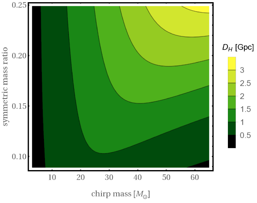
Figure 1.— Horizon distance in Gpc for nonspinning BBHs as a function of chirp mass and symmetric mass ratio assuming a single detector with the early aLIGO noise spectrum.

3.2. Cosmological effects

We simulate an expanding universe with sources distributed uniformly and isotropically in comoving volume, which on scales of hundreds of Mpc is a valid assumption. Since the frequencies of any signal become increasingly redshifted with growing distance between source and detector, the total chirp mass measured at the detector is shifted by

$$\mathcal{M}^{\ast}=\mathcal{M}\,(1+z),$$ (7)

where $z$ denotes the redshift. Assuming zero curvature and standard cosmological parameters (Bennett et al., 2014)

$$\Omega_{M}=0.286,\quad\Omega_{\Lambda}=1-\Omega_{M},\quad H_{0}=69.6,$$ (8)

we calculate the comoving distance as a function of the redshift (Hogg, 1999),

$$D_{C}(z)=\frac{c}{H_{0}}\int_{0}^{z}\frac{dz^{\prime}}{\sqrt{\Omega_{M}(1+z^{\prime})^{3}+\Omega_{\Lambda}}}.$$ (9)

Here, $c$ denotes the speed of light.

The catalogues by Dominik et al. (2012) provide large sets of binaries characterized by their intrinsic chirp mass $\mathcal{M}$ and symmetric mass ratio $\eta$. When we distribute them uniformly in comoving volume, the observed chirp masses $\mathcal{M}^{\ast}$ are redshifted according to (7). This implies that the maximal distance to which they can be detected changes as it is the observed parameters, not the intrinsic parameters, that determines the appropriate horizon distance. Since

$$D_{L}=D_{C}(1+z),$$ (10)

the maximal observable comoving distance satisfies

$$D_{C}^{\rm max}(\mathcal{M},\eta,z)\;(1+z)=D_{H}(\mathcal{M}^{\ast},\eta),$$ (11)

which we solve numerically for $z$. Note that the leading-order inspiral horizon distance behaves as $D_{H}(\mathcal{M}^{\ast})\sim(\mathcal{M}^{\ast})^{5/6}$, hence

$$D_{C}^{\rm max}(\mathcal{M})\sim\frac{\mathcal{M}^{5/6}}{(1+z)^{1/6}}<D_{H}(\mathcal{M}).$$ (12)

While the derivation of (12) is only valid for low-mass systems, we find that $D_{C}^{\rm max}$ is generally less than the static, Euclidean universe equivalent $D_{H}$.

3.3. Detection rate and distance distribution

We now assume binaries of a fixed model, distributed isotropically and uniformly in comoving volume, that merge at a constant comoving merger rate density $\mathcal{R}$ (in $\text{MWEG}^{-1}\;\text{Myr}^{-1}$) as given in the data sets by Dominik et al. (2012). To convert these numbers into a detection rate for aLIGO, we proceed as follows:

First, the comoving merger rate $\mathcal{R}$ per MWEG has to be multiplied by an average galaxy density which we take as $\rho_{G}\approx 0.0116\,\text{Mpc}^{-3}$ following Kopparapu et al. (2008). Next, we must calculate the effective volume in which each binary is observable, by integrating the number of observable binaries as a function of $D_{C}$. As the distance increases, the area of the corresponding sphere increases as $D_{C}^{2}$ but the fraction of binaries that are oriented such that their signal is sufficiently loud for detection (that is, $D_{\rm eff}<D_{H}$) becomes smaller. Finally, due to the redshifted time,

$$t_{L}=t_{C}(1+z)$$ (13)

the observed merger rate for binaries at redshift $z>0$ is less than the comoving merger rate. Thus, the effective volume for a binary with chirp mass $\mathcal{M}$ is

$$V_{\rm eff}(\mathcal{M})=4\pi\int_{0}^{D_{C}^{\rm max}}\frac{D_{C}^{2}}{1+z}\;P\!\left(\frac{D_{L}}{D_{H}(\mathcal{M}^{\ast},\eta)}\right)dD_{C}\,,$$ (14)

where $D_{C}^{\rm max}$ is defined by (11). The function $P$, introduced in Eq. (6), gives the fraction of suitably oriented binaries (i.e., those giving an SNR greater than 8) and $(1+z)^{-1}$ accounts for the difference between apparent and comoving merger rate density. We note that the integrand in (14) can be interpreted (up to a normalisation) as the observed distance distribution for binaries with fixed intrinsic parameters.

The average detection rate for each model is given by

$$\dot{N}=\mathcal{R}\times\rho_{G}\times\overline{V_{\rm eff}},$$ (15)

where $\overline{V_{\rm eff}}$ denotes the average effective volume, with the average taken over all binaries in a given model. We take $\mathcal{R}$ and $\rho_{G}$ from Dominik et al. (2012) and Kopparapu et al. (2008), respectively.

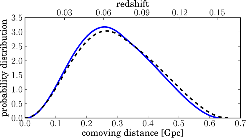
Figure 2.— The probability distribution in comoving distance for detectable BBHs with $m_{1}=m_{2}=10M_{\odot}$. The solid (blue online) curve takes cosmological effects into account (see text) while the dashed line assumes a static, Euclidean universe (i.e. local universe approximation).

Figure 2 shows this distribution for an equal-mass BBH with $m_{1}=m_{2}=10M_{\odot}$. For comparison, we include the equivalent curve for a static, Euclidean universe, where $D_{L}\equiv D_{C}$ and (14) simplifies to the case $z=0$. As expected, both curves agree for low redshift, but as we have noted above, there are fewer binaries seen at large comoving distances if the expansion of the universe is taken into account. This effect becomes increasingly important for larger distances, i.e., for high-mass binaries and more sensitive detector configurations.

The effective volume in which binaries with fixed parameters are detectable changes considerably across the parameter space. This leads to an observational bias in favour of systems with large volume reach. We incorporate this effect by re-weighting the chirp mass distribution of binaries according to their individual effective volumes. In practice, Dominik et al. (2012) provide the data for each of their models in form of a discrete set of binary parameters. For each of those binaries, we calculate the integer part of $V_{\rm eff}/V_{\rm eff}^{\rm min}$ and add that many copies of the binary to our new set of observable parameters. Here, $V_{\rm eff}^{\rm min}$ denotes the smallest effective volume across all binaries in the set, and only one copy of the binary with this smallest effective volume is kept.

Finally, for each binary in our new set, we draw a comoving distance from the distribution underlying $V_{\rm eff}$. From this distance, we then infer the redshift and change from $\mathcal{M}$ to the observable redshifted chirp mass $\mathcal{M}^{\ast}$ according to (7). Our discrete representation of observable binaries then consists of multiple copies of the same intrinsic systems, each however with a unique redshifted chirp mass.

Note that an equivalent, but computationally more expensive, procedure would be to randomly draw binaries from the intrinsic distribution, then draw comoving distances and orientations for each binary within the total sensitive volume for the respective model and only keep those binaries with a detectable GW signal. Our method instead avoids disregarding any randomly drawn sources by drawing from the appropriate (distance/orientation) distribution of detectable signals.

3.4. Estimating and Including Measurement Errors

Including the observational bias discussed in Sec. 3.3 in the chirp mass distribution still does not yield the distribution that one would expect to observe, because there will be a measurement error associated with each of the observations. Previous publications have mainly discussed a full Bayesian framework to combine multiple observations including their measurement uncertainties (Mandel, 2010; Mandel & O’Shaughnessy, 2010; O’Shaughnessy, 2013). We instead assume a statistical fluctuation of the measured parameter around its true value as detailed below.

The accuracy of the parameters recovered during GW searches is limited by two factors. First, since we match to templates of the signals, the accuracy of recovered parameters will be limited by the accuracy of the waveform models that used in the search. Second, the accuracy will be affected by statistical fluctuations of the noise in the measurement process. While we leave the former for dedicated studies such as Buonanno et al. (2009) and Nitz et al. (2013), we can estimate the uncertainty due to the latter using the well-known Fisher matrix estimate.

Fisher matrix analyses rely on a linear approximation of signal variations and are valid for large SNRs. Neither of the two assumptions is typically valid in realistic scenarios, and recent papers have discussed some implications of violating these assumptions (Vallisneri, 2008; Rodriguez et al., 2013; Mandel et al., 2014). Here, however, in order to demonstrate the basic efficacy of our method to distinguish BBH populations with GW observations, we take Fisher-matrix predictions as a proxy for the width of posterior distributions of parameters obtained via a fully Bayesian analysis of the kind that will be performed on actual GW events (Veitch et al., 2014). In performing a population study of the kind we perform here, one should include not only a point estimate for parameters such as the chirp mass, but the full posterior from these parameter estimation routines. These posteriors can then be combined in the correct way, as described in Mandel (2010). The method we use here is essentially the point estimate approximation to the full analysis.

We employ the same inspiral-merger-ringdown model (Santamaría et al., 2010) for our Fisher-matrix calculations as we used to simulate GW signals. We only consider variations of the intrinsic parameters: masses, time, phase and a model-specific single effective spin. We assume that these are also the parameters that are recovered, at least initially by the GW search algorithm (see, e.g., the recently proposed search algorithm for nonprecessing, spinninng binaries by Dal Canton et al. (2014)). This assumption is likely to make our error estimates too large since actual GW events will be followed up by complex parameter estimation routines (see e.g., Veitch et al. (2014)) exploring the full parameter space of precessing binaries (Vitale et al., 2014; Chatziioannou et al., 2015; O’Shaughnessy et al., 2014). However, since we only need an approximate error estimate that can be obtained in a fast and reliable way across the BBH parameter space, we choose to use the Fisher-matrix method here for nonprecessing binaries, and we neglect small correlations with extrinsic parameters such as sky location, orientation or distance.

The characteristic standard deviations in the measurement process are estimated by (Poisson & Will, 1995)

$$\Delta\theta^{i} = \sqrt{(\Gamma^{-1})_{ii}},$$ (16)

$$\Gamma_{ij} = \left(\frac{\partial h}{\partial\theta^{i}},\frac{\partial h}{\partial\theta^{j}}\right),$$ (17)

where $\Gamma_{ij}$ is the Fisher information matrix and $h=h(\theta^{i})$ is the waveform model. The inner product used in (17) is given by

$$\left(g|h\right)=4\operatorname{Re}\int_{f_{\rm low}}^{\infty}\frac{\tilde{g}(f)\tilde{h}^{*}(f)}{S_{n}(f)}df$$ (18)

which is consistent with the SNR definition in (3). The form of the waveform model we use allows us to calculate the partial derivatives used in the definition of $\Gamma_{ij}$ analytically, and we ensure numerical errors in the matrix inversion remain small.

The only parameter we use to distinguish BBH populations in this study is the observable, redshifted chirp mass, $\mathcal{M}^{\ast}$. The data sets of expected observable chirp masses that we prepared following the algorithm introduced in Sec. 3.3 shall now be skewed further by adding measurement errors to each binary in the data set. We do so by assuming a Gaussian distribution centred around the chirp mass value of each binary with a standard deviation given by the Fisher matrix estimate (16). We evaluate the Fisher matrix at the appropriate observed chirp mass and mass ratio of the binary, setting the value of the black hole spins to zero (although we allow the spins to vary when calculating the Fisher matrix). This has a negligible effect on our results as the measurement accuracy for the chirp mass is only weakly dependent on the spins (Ohme et al., 2013). We randomly draw a sample from this distribution to re-define the measured chirp mass. Similarly, when we later simulate the universe with a particular model, each observation is drawn from the distribution that incorporates observational biases, but the actually measured chirp mass is additionally offset following the Gaussian distribution that simulates measurement errors.

The Fisher-matrix estimates scale inversely with the SNR, so we only calculate them once across the parameter space and scale them for each binary in the data set according to its SNR, which in turn is inferred from the distance and a randomly chosen orientation. Figure 3 shows the chirp mass uncertainty at a constant SNR of 10 across the parameter space for the early configuration of aLIGO.

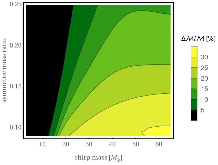
Figure 3.— Expected relative measurement errors in the chirp mass for an early configuration of aLIGO, SNR 10, calculated using the PhenomC waveform model (Santamaría et al., 2010).

Figure 4 illustrates the transition from the intrinsic BBH population, predicted by Dominik et al. (2012) for each of their models, to the expected observed chirp mass distribution. The main effect of the observational bias detailed in Sec. 3.3 is that the distribution becomes skewed towards high-mass binaries, and its support extends to larger chirp masses due to the redshift of distant sources. The addition of measurement errors hardly affects the distribution at low chirp masses, simply because the errors are small compared to the typical variation of the distribution in this regime. For heavy systems, on the other hand, noise fluctuations introduce a non-vanishing chance of measuring chirp mass values greater than the largest (redshifted) chirp mass in each model. Hence, the main effect of introducing measurement errors is that the expected observed distributions show a characteristic tail at high chirp masses.

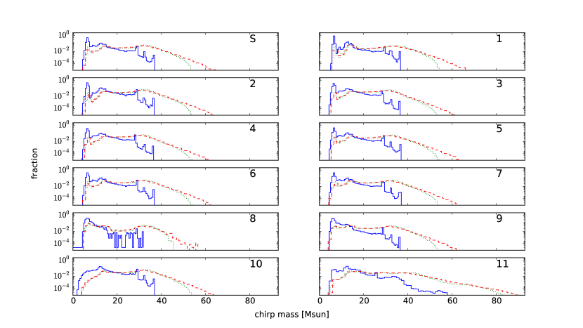
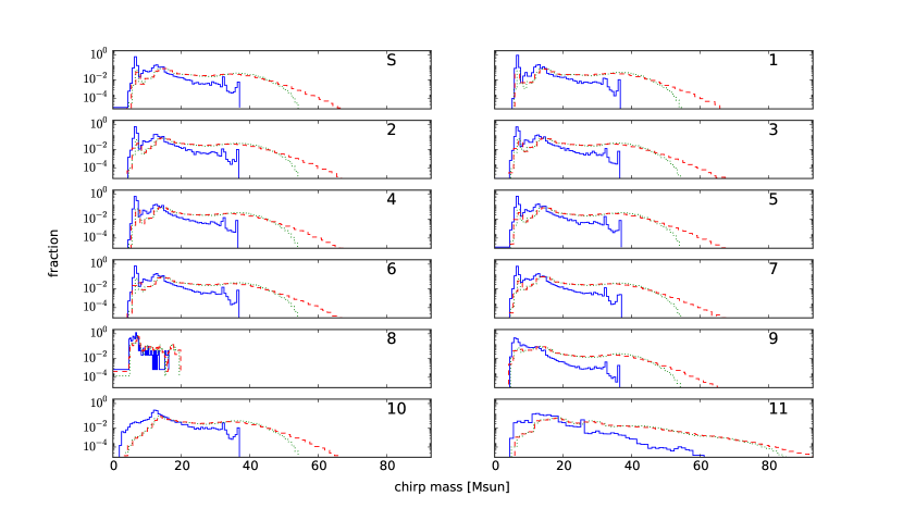
Figure 4.— Chirp-mass distributions for each model in Dominik et al. (2012) using either their optimistic (top panel) or pessimistic (bottom panel) submodel and a 50-50 split of solar and sub-solar metallicities. The solid (blue online) line shows the intrinsic distribution as given by Dominik et al. (2012). The dotted (green) line shows the same distribution when accounting for the observational biases introduced in Secton 3.3 as predicted for the early configuration of aLIGO. Finally, the dashed (red) line with largest chirp-mass support shows the expected observed distribution that additionally folds in the errors in measuring the chirp masses through GW observations.

4. Combining Measured Rates and Chirp Masses

Given a set of BBH observations, for each model variation $V_{i}$, we wish to calculate the posterior probability for that being the correct model. The information we gather about the correct model is twofold. First, we obtain a set of observed chirp masses $\{\mathcal{M}\}$, and second, we measure the rate of BBH detections by observing $n$ binaries in a given observation period. In reality each observation will include measurements of additional physical parameters of the system, such as the component spins (see Gerosa et al. (2013, 2014) for information on how measurements of spin misalignments can help to constrain astrophysical formation scenarios.) Including additional information from these other dimensions should help in distinguishing astrophysical formation scenarios.

We simulate the observed population by choosing one of the model variations, adjusted to account for selection effects as described above, to describe the universe. We then draw $n$ individual chirp mass measurements from this model, which form the data $\{\mathcal{M}\}$. The number of observations we assume is itself drawn from a Poisson distribution with a mean value that is dictated by the observation time and the merger rate of the model variation we have selected to simulate the universe.

With these measurements, $\{\mathcal{M}\}$ and $n$, the posterior probability that model $V_{i}$ is the correct model reads

$$P(V_{i}|\{\mathcal{M}\},n)=\frac{P(\{\mathcal{M}\},n|V_{i})P(V_{i})}{P(\{\mathcal{M}\},n)},$$ (19)

where we have used Bayes’ Theorem. $P(V_{i})$ is the prior probability on model $V_{i}$, $P(\{\mathcal{M}\},n|V_{i})$ is the likelihood of making these chirp mass measurements and measuring this detection rate given model variation $V_{i}$, and $P(\{\mathcal{M}\},n)$ is a normalisation factor called the evidence.

Assuming that the number of observations $n$ is independent from the chirp mass values we observe, we can rewrite this as

$$P(V_{i}|\{\mathcal{M}\},n)=\frac{P(\{\mathcal{M}\}|n,V_{i})P(n|V_{i})P(V_{i})}{P(\{\mathcal{M}\},n)}.$$ (20)

We normalise by assuming that the discrete model variations we consider cover all possible states of the universe, which is an idealisation that we shall discuss in more detail later. However, this assumption allows us to define the normalisation factor by requiring the sum of the probabilities for each model to be unity, which leads to

$$P(V_{i}|\{M\},n)=\frac{P(\{M\}|n,V_{i})P(n|V_{i})P(V_{i})}{\sum_{k}P(\{M\}|n,V_{k})P(n|V_{k})P(V_{k})}.$$ (21)

We assume a uniform prior on the models,

$$P(V_{i})=\frac{1}{\mathcal{N}},$$ (22)

where $\mathcal{N}$ is the number of models we are considering. The prior then cancels out and we are left with

$$P(V_{i}|\{\mathcal{M}\},n)=\frac{P(\{\mathcal{M}\}|n,V_{i})P(n|V_{i})}{\sum_{k}P(\{\mathcal{M}\}|n,V_{k})P(n|V_{k})}.$$ (23)

The likelihood of making $n$ observations in a set time, given a model predicting mean number of observations, $\mu_{i}$, is given by the Poisson distribution:

$$P(n|V_{i})=P(n|\mu_{i})=\frac{e^{-\mu_{i}}\mu_{i}^{n}}{n!}.$$ (24)

The likelihood terms of the form $P(\{\mathcal{M}\}|n,V_{i})$ are calculated by binning the chirp mass distributions for each model into a histogram. We then calculate the likelihood of the observed samples being drawn from their bins using the multinomial distribution

$$P(\{\mathcal{M}\}|n,V_{i})=n!\prod_{k=1}^{b}\frac{p_{ik}^{x_{k}}}{x_{k}!},$$ (25)

where $n$ is the number of samples in the observations, $b$ is the number of bins, $p_{ik}$ is the probability in model $i$ of drawing a sample from bin $k$ and $x_{k}$ is the number of observations that fall into bin $k$, with

$$\sum_{k}x_{k}=n\quad\textrm{and}\quad\sum_{k}p_{ik}=1.$$ (26)

We calculate $p_{ik}$ for each model and bin as the fraction of the total number of samples in the model which fall into that bin. The bin size we employ is motived by Scott’s rule (Scott, 1979),

$$\Delta=\frac{3.5\sigma}{\sqrt[3]{N_{m}}},$$ (27)

where $\Delta$ denotes the bin width, $\sigma$ is the standard deviation of the model, and $N_{m}$ is the total number of samples in model. To be able to consistently compare our simulated data with all models, we apply (27) to all models and then use the median bin width for the actual analysis. However, we find that changing this bin width by a factor of a few does not impact our results noticeably.

5. Observing Scenarios

The method we have developed transforms predicted binary distributions and merger rates into observable distributions and detection rates which in turn can be confronted with a set of observations in order to assign posterior probabilities to each model. As such, the method is generally applicable to any set of theoretical predictions and detector configuration.

In the following, however, we present results for specific choices of binary population models, detector sensitivity and observing time. As detailed Sec. 2.2 and summarised in Table 1, we consider 12 binary population models by Dominik et al. (2012), each with both the “pessimistic” (submodel B) and “optimistic” (submodel A) assumption about the common envelope evolution. This leads to 24 distinct predictions of the BBH chirp mass distribution (see Figure 4), where each comes with a distinct average merger rate density that we take from the arithmetic mean of the solar and subsolar metallicity predictions by Dominik et al. (2012) (Tables 2 and 3 therein). The local merger rate densities for each model are given in Table 2. Interestingly, due to the mass-dependent observational bias, models with higher merger rate density do not necessarily exhibit a higher detection rate, see for instance models 9 and 10 in Table 2.

Recent calculations by Dominik et al. (2013) that include the cosmological evolution of merger rates give lower rate densities than the ones we infer from earlier work of the same authors. Consequently, the detection rates we find are up to a factor of 2 larger than those recently predicted by Dominik et al. (2014) (this is based on a direct comparison of our method with their otherwise equivalent approach using the same detector configuration). However, this neither affects the general proof of principle carried out here, nor do the conclusions we shall draw in the following section change qualitatively by varying the detection rate at this level.

Table 2Predicted merger and detection rates.

	$\bm{\mathcal{R}}$		$\bm{\langle\mathcal{M}\rangle}$		$\bm{\mu}$ (O1)		$\bm{\mu}$ (O2)
$\bm{V_{i}}$	B	A	B	A	B	A	B	A
0	7.8	40.8	26.0	24.9	4.0	25.2	64	402
1	4.6	6.8	27.3	26.2	2.3	3.9	37	63
2	8.3	36.0	26.6	24.9	4.2	25.9	67	413
3	4.0	47.6	25.0	24.4	1.9	28.7	30	458
4	0.1	3.1	25.0	24.7	0.1	1.9	1	30
5	7.8	40.9	26.0	24.9	4.0	25.3	64	404
6	7.9	41.3	25.6	24.2	3.9	25.1	63	401
7	8.6	47.1	25.3	23.8	4.0	26.3	65	420
8	0.4	2.1	21.3	10.0	0.0	0.6	1	9
9	11.8	54.6	23.2	20.7	3.4	20.2	54	324
10	5.8	31.3	26.8	26.2	4.3	26.0	68	415
11	10.4	54.5	29.8	28.6	8.5	46.5	136	742

Note. — The binary populations models, $V_{i}$, predicted by Dominik et al. (2012) are summarised in Table 1 and the submodels B and A refer to pessimistic and optimistic assumptions about the common envelope evolution of Hertzsprung gap donors (Sec. 2.2.2).

We also have to specify in the sensitivity (i.e., noise spectral density) of our assumed GW detector and the observing time. Closely following Aasi et al. (2013b), we consider the first two aLIGO science runs dubbed O1 and O2, respectively. The first science run for aLIGO (O1) is planned to begin in autumn 2015. The duration of O1 will be approximately 3 months for the two aLIGO detectors. We assume each detector has a duty cycle of 0.8 so that the total period of coincident observation during O1 will be about 0.16 years. The noise power spectral density we use is the “early aLIGO” configuration (Shoemaker, 2010).

We further consider a second science run, O2. During O2, the detectors are planned to observe for approximately 6 months with a comparable duty cycle to O1. It is expected that, after further improvements of the instruments following O1, the aLIGO detectors during O2 will be approximately a factor of 2 more sensitive than the nominal early aLIGO noise curve we use for O1. While the evolution of the noise power spectral density is in general a function of the frequency, we find that, in practice, the difference between the predicted noise curves in Aasi et al. (2013b) results in improved horizon distances and error estimates that are well approximated by simply scaling the results we obtain for the early aLIGO configuration. Hence, we simulate O2 by multiplying the O1 horizon distance by 2. The Fisher-matrix errors change only due increased SNR at fixed distance. This increase in sensitivity leads to a factor of 8 increase in volume meaning that, in total, O2 surveys 16 times the time-volume of O1. We show in the following section that this is when we will begin to distinguish between astrophysical models.

6. Results: Distinguishing BBH Formation Models

6.1. First aLIGO observing run (O1)

We simulate the observed BBH systems, assuming the universe matches one of the models from Dominik et al. (2012), and calculate the posterior probability for each model. We repeat the experiment 10000 times before turning to the next model to simulate the universe. Figure 5 gives the median posterior probability for each model.

In cases where one or few models have a high probability, these would be distinguishable from the other models. However, all models with a high probability would be consistent with the observations. We reiterate that here we restrict attention to the models in Dominik et al. (2012). Of course these do not cover the full space of binary merger predictions. If we were to include a broader range of models, it is likely that the conclusions we are able to draw would be weaker as various models would lead to comparable rates and mass distributions. Nonetheless, some of the conclusions we reach, such as excluding a number of models if there are no observations in O1, are robust.

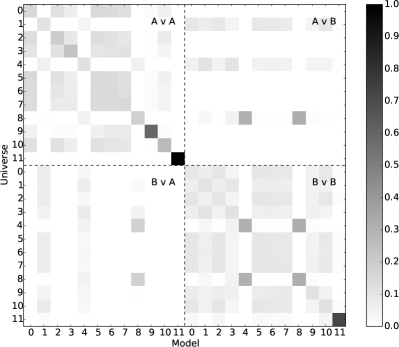
Figure 5.— The median posterior probability for each model in the set of Dominik et al. (2012) models after an O1 like observing period of 0.16 years, calculated from 10000 repeats. The model which observations were drawn from is shown on the axis labelled Universe. The models which these observations were then compared to is labelled Model, so that the probabilities in each row sum to one. Models 0-11 are described in Table 1. The two submodels, A and B, are described in Section 2.2.2.

We first observe that, for the most part, we would be able to distinguish between submodels A and B that correspond to different common envelope scenarios (see Sec. 2.2.2). This is unsurprising as the predicted rates for the majority of models are significantly higher for submodel A (cf. Table 2). Models which predict low detection rates for model A remain degenerate with those in model B. The mass distribution from such a small sample does not provide enough additional information to break these degeneracies in the rates. For example, model 1 A uses a very high, fixed envelope binding energy, meaning that most binaries entering a common envelope event fail to throw off the common envelope and merge, causing them to never form BBH systems (for a more detailed discussion of this, see Dominik et al. (2012)). On the other hand, submodel B does not allow a binary to survive a common envelope event if the donor is on the Hertzsprung Gap, and so again, many binaries merge and never form BBHs. This generically lowers the merger rates and thus detection rates for submodel B models, leading to the degeneracy visible in the upper right quadrant of Fig. 5.

Another interesting example involves models 4 and 8 that, in the pessimistic submodel B, are consistent with no observations at all during O1. Hence, they cannot be distinguished from each other, or indeed model 8 A, although they are favoured over all other models if indeed no detection are made.

Within the two submodels, it is difficult to identify the correct model. Indeed, there are numerous variations which would be indistinguishable from the standard model. The only model which can be clearly identified is model 11, a model which reduces the strength of stellar winds by a factor of 2 over the standard model. We now discuss why we are able to distinguish this model from the others in such a short observational period.

6.2. Stellar winds

In massive O-type stars, stellar winds of high temperature charged gas are driven by radiation pressure. In Wolf–Rayet stars mass loss rates can be as high as $10^{-4}\mbox{M${}_{\odot}$}\text{yr}^{-1}$ (Nugis & Lamers, 2002). This can cause stars to lose a large amount of mass prior to the supernova. Theoretical uncertainties in modelling these mass loss rates therefore translate into uncertainties in the pre-supernova masses for massive stars. Dominik et al. (2012) examine the effects of reducing the strength of stellar winds by a factor of 2 on the distribution of BBHs in their Variation 11. Firstly, reducing stellar winds results in stars having a higher mass prior to supernova than they would otherwise have. This in turn leads to more mass falling back onto the compact object during formation, which reduces the magnitude of natal kicks given to black holes. This results in more systems surviving the supernova (rather than being disrupted) and increases the merger rates. More massive pre-supernova stars also form more massive remnants, resulting in the most massive BBH having a chirp mass of $\sim 64\mbox{M${}_{\odot}$}$ with reduced stellar winds compared to $\sim 37\mbox{M${}_{\odot}$}$ using the standard prescription. Finally, reducing the strength of stellar winds allows stars with a lower zero age main sequence mass to form black holes due to more mass being retained. This can boost the BBH merger rate compared to the standard model.

All of these effects combined mean that Variation 11 predicts BBHs with characteristically higher chirp masses, as well as predicting a much higher merger rate than all other models (even for the pessimistic submodel B in O1, Variation 11 predicts $\mathcal{O}(10)$ observations). We therefore expect that we would be able to correctly distinguish a universe following Variation 11 from all other models with relatively few observations. In Figure 6 we show the median posterior probability for each model as a function of the observation time, based on 10000 redraws of the observations. We find that when drawing observations from a universe following Variation 11 we overwhelmingly favour it within the duration of O1, with $\mathcal{O}(10)$ observations.

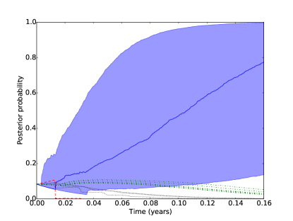
Figure 6.— The median posterior probability for each of the models in the set as a function of observation time for a period of time corresponding to the aLIGO O1 run (0.16 years). GW observations are drawn from a universe following Variation 11, submodel B which reduces the strength of stellar winds by a factor of 2 compared to the standard model. The blue (solid) line shows the median posterior probability for Variation 11 taken from 10000 repeats, and the shaded error bar shows the 68% confidence interval. Variations 0,2,5,6,7 & 10 are plotted in green (dot-dash), while variations 1,3 & 9 are plotted in black (dotted). Variations 4 & 8 predicting $\sim 0$ observations in O1 are plotted in red (dashed).

6.3. Second aLIGO observing run (O2)

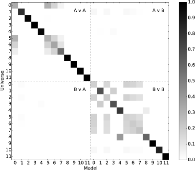
Figure 7.— The median posterior probability for each model in the set of Dominik et al. (2012) models after an O2 like observing period of 0.32 years with a detector more sensitive than the early aLIGO noise curve by a factor of 2. The median is calculated based on 10000 redraws of the observations. The model which observations were drawn from is shown on the axis labelled Universe. The model which these observations were then compared to is labelled Model. Models 0-11 are described in Table 1. The two submodels, A and B, are described in Section 2.2.2.

We now turn our attention to the second observing run, O2, and investigate which models can be distinguished using the much larger time-volume surveyed by O2. In Figure 7 we again show a matrix plot showing the (median) posterior probability for each model after a period corresponding to the O2 run.

Figure 7 has a more diagonal form than Figure 5, meaning that in many cases the correct model is favoured and others are disfavoured within the O2 period. In particular, the optimistic and pessimistic submodels A and B become almost entirely distinct from each other. This is because most of the Dominik et al. (2012) models predict $\mathcal{O}(100)$ ($\mathcal{O}(10)$) observations during the O2 period for the optimistic (pessimistic) submodels respectively (as shown in Table 2). Furthermore, the majority of variations in submodel A can be unambiguously identified; the exception being that the standard model which remains degenerate with models 5, 6 and 7, as we discuss in detail in Section 6.3.1. For the pessimistic submodel B, the standard model remains indistinguishable from a number of other variations. However, there are a few models which can be clearly distinguished, including models 4 and 8 (that predict significantly lower rates), and 9, 10 and 11. All of these models predict tens of observations and consequently, we are able to use information from both the chirp mass distribution and the detection rate to help distinguish models. Model 10 involves the variation of the supernova engine, which we elaborate on in Section 6.3.2.

6.3.1 Black hole kicks and maximum neutron star mass

Not all models are distinguishable, even with the $\mathcal{O}(100)$ observations predicted by the optimistic submodel A for O2. For example, in Figure 7 we see that the standard model is degenerate with Variations 5, 6 and 7. We now explain why this is so.

As already mentioned, it is unclear what the correct distribution of natal kicks given to black holes upon formation is. In order to investigate the possibilities, Dominik et al. (2012) vary two parameters relating to the kicks imparted onto newly formed black holes; the characteristic velocity $\sigma$ and the fraction of mass $f_{b}$ which falls back onto the newly born black hole.

In their standard model, black holes receive a kick $v_{k}$ whose magnitude $v_{\text{max}}$ is drawn from a Maxwellian distribution with $\sigma=265\text{km s}^{-1}$, and reduced by the fraction of mass falling back onto the black hole $f_{b}$ as

$$v_{k}=v_{\text{max}}(1-f_{b}),$$ (28)

where $f_{b}$ is calculated using the prescription given in Fryer et al. (2012).

In order to test the effects of smaller natal kicks, in Variation 7 Dominik et al. (2012) reduce the magnitude of kicks given to neutron stars and black holes at birth by a factor of 2. They use a Maxwellian distribution with $\sigma=132.5\text{km s}^{-1}$. For BBHs, this has very little effect on the chirp mass distribution, and so one cannot expect to be able to distinguish this model from one using full kicks.

The same holds true when the maximum neutron-star mass is increased (decreased) from its fiducial value in the standard model of $2.5\mbox{M${}_{\odot}$}$. This has very little impact on the BBH chirp mass distribution and so there is effectively a degeneracy between these models. This could be resolved by also including BNS observations in the comparison. We do not do this here as we concentrate on the BBH predictions, due to the prediction by Dominik et al. (2012) that these will dominate the early aLIGO detections.

6.3.2 Supernova engine

In their standard model, Dominik et al. (2012) employ the Fryer et al. (2012) prescription to calculate the fraction of mass falling back onto the black hole during formation, and thus the black hole masses. In particular, they use the rapid supernova engine. When employed in a compact binary population code such as StarTrack, the rapid supernova engine reproduces the observed mass gap (Ozel et al., 2010; Farr et al., 2011) in compact objects between the highest mass neutron stars and the lowest mass black holes (for a discussion of using GW observations to infer the presence or absence of a mass gap, see Hannam et al. (2013); Littenberg et al. (2015); Mandel et al. (2015)).

In model 10 Dominik et al. (2012) vary this prescription to use the delayed supernova engine from Fryer et al. (2012), which produces a continuous distribution of black hole masses (and thus BBH chirp masses). We therefore expect that the difference between these two models might be visible in the chirp mass distributions. We see however from Table 2 that these two models predict similar merger rates for BBH, and so we do not expect to be able to distinguish them based on the detection rate. Nonetheless, we see from Figure 7 that this model can be distinguished from the others by the end of O2 and even, to a lesser degree, at the end of O1 (Figure 5)

Rates only	Mass distribution only

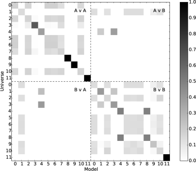
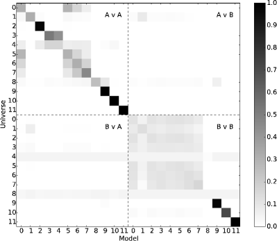
Figure 8.— Probabilities for the scenario of Fig. 7, separated into contributions from the rates (left) and the mass distribution (right).

To illustrate the importance of both the mass distribution and predicted rates, in Figure 8 we show the results that would be obtained using only one of these to separate the models. By comparing these results with Figure 7, it becomes clear that both the mass and rate measurements contribute significantly to our ability to distinguish between models. As expected, the delayed supernova engine (model 10) is distinguished from observed masses, but the rates are quite degenerate with other models. In contrast, models 4 and 8, are distinguished primarily by rate measurements, and not masses. As we have mentioned previously, the unknown spin distribution of black holes in binary systems can change the rate by a factor of two or three. Similarly, both the mass and rate distributions are subject to uncertainties due to additional physical effects which are not yet incorporated. Consequently, one might choose to incorporate an uncertainty in the rates or mass distributions. The results in Figure 8 illustrate the extreme scenario where one assumes knowledge of only the rate or mass distribution. Adding an uncertainty to the mass or rate distributions will lead to a result between those shown in Figure 7 and 8.

7. Summary and future work

In this paper we have outlined a method for comparing GW observations of BBH mergers to binary population synthesis predictions using a Bayesian model comparison framework. Starting from chirp mass distribution predicted by Dominik et al. (2012), we produce predicted observed chirp mass distributions accounting for known observational effects. We incorporate

1. The redshifting of observed binary masses due to the cosmological distances out to which they will be observed.

2. The observational bias of GW detectors to detect more massive systems, since they can be seen to greater distances and thus in much larger volumes.

3. Fisher matrix estimates of measurement uncertainties in the recovery of the chirp mass of BBH.

We show that given the merger rates predicted by the models of Dominik et al. (2012), we will begin to be able to distinguish between population synthesis models in the first two aLIGO science runs. Ruling out models in turn can help to constrain the value of unknown parameters, which relate to poorly understood astrophysics relating to binary evolution.

Of course, the set of models considered here by no means encompasses the full set of stellar evolution models available in the literature. We restricted attention to this subset of models as the data was publicly available in an easy to use form. It would be straightforward to include additional models into this analysis. Ideally, we would make use of a dense set of models, where numerous astrophysical parameters are jointly varied. This would allow us to interpolate between models, and extract best-fit parameters (O’Shaughnessy, 2013; O’Shaughnessy et al., 2008). Furthermore, we have restricted attention to the two best-measured quantities: the rate and chirp mass distribution of binaries, and only used point estimates of the masses. The inclusion of full parameter distributions can only enhance our ability to distinguish between models.

The method we have introduced allows us to distinguish between a given set of stellar evolution models. It will identify the model, or models, that best agree with the observed rate and mass distribution. It will not, however, indicate whether the best model is actually a good fit to the observations — only that it is better than the others. This could be remedied by introducing a simple, generic model. For example, the intrinsic mass distributions shown in Figure 4 are reasonably well desribed by a decaying power law with an upper and lower mass cutoff. One could then imagine extending the set of models to include this phenomenological mass distribution parametrized by three variables with an additional variable rate. To calculate the posterior for this distribution, we would then have to marginalize over four parameters. Thus, even if the generic model was a reasonable fit to the data, it would be penalized by the large initial parameter space. It is likely that the generic model would be preferred after a small number of observations. With a large number of observations, the rate and mass distributions would be reasonably well measured. Any specific model which matched the observations well would then be preferred to the generic model due to its broader support on the parameter space. It would be reasonably straightforward to extend our method to include a generic model, and this is something we plan to incorporate in the future.

In this study we concentrated on the information that could be gained from GW observations of BBH mergers. aLIGO and AdV are also expected to observe the inspiral, merger and ringdown of compact binaries including neutron stars (BNS and NSBH systems). One should include all GW observations of compact binaries in order to extract the maximum amount of information from the observations. In fact, as discussed above, we are unable to distinguish models which vary the maximum allowed neutron star mass since we ignore these events here. In this study we ignored these events since the predicted detection rates for BBH mergers dominated those of other compact binary mergers. The BBH mass distribution also spans a large range of masses, with structure encoding information about binary evolution. Ignoring other families of compact binaries also allowed us to avoid ambiguities in discerning the family of the source (BNS, NSBH or BBH) due to degeneracies which exist in measuring the mass ratio for these systems (Hannam et al., 2013), although this can be dealt with in the future (Farr et al., 2013).

All these considerations have to be carefully taken into account in future studies. However, our results indicate that the upcoming generation of advanced GW detectors will soon start putting non-trivial bounds on current and future binary evolution models, and analyses like the one presented here will provide an important basis to link theoretical models with GW observations.

References

- Aasi et al. (2010) Aasi, J., et al. 2010, Possible scenarios for Commissioning and Early observing with the Second Generation Detectors, Tech. Rep. LIGO-G1000176
- Aasi et al. (2013a) —. 2013a, Phys.Rev., D88, 062001
- Aasi et al. (2013b) —. 2013b, arXiv:1304.0670
- Aasi et al. (2013c) —. 2013c, Phys. Rev. D 87,, 022002, 022002
- Aasi et al. (2014) —. 2014, Phys.Rev.Lett., 113, 011102
- Aasi et al. (2015) Aasi, J., Abbott, B. P., Abbott, R., et al. 2015, Classical and Quantum Gravity, 32, 074001
- Abadie et al. (2010) Abadie, J., et al. 2010, Class.Quant.Grav., 27, 173001
- Abadie et al. (2012a) —. 2012a, A&A, 541, A155
- Abadie et al. (2012b) —. 2012b, Phys.Rev., D85, 082002
- Acernese et al. (2015) Acernese, F., et al. 2015, Class.Quant.Grav., 32, 024001
- Ajith et al. (2011) Ajith, P., Hannam, M., Husa, S., et al. 2011, Phys.Rev.Lett., 106, 241101
- Antoniadis et al. (2013) Antoniadis, J., Freire, P. C. C., Wex, N., et al. 2013, Science, 340, 448
- Babak et al. (2013) Babak, S., Biswas, R., Brady, P., et al. 2013, Phys.Rev., D87, 024033
- Belczynski et al. (2013) Belczynski, K., Bulik, T., Mandel, I., et al. 2013, Astrophys.J., 764, 96
- Belczynski et al. (2010) Belczynski, K., Dominik, M., Bulik, T., et al. 2010, arXiv:1004.0386
- Belczynski et al. (2012) Belczynski, K., Dominik, M., Repetto, S., Holz, D. E., & Fryer, C. L. 2012, ArXiv e-prints, arXiv:1208.0358
- Belczynski et al. (2008) Belczynski, K., Kalogera, V., Rasio, F. A., et al. 2008, Astrophys.J.Suppl., 174, 223
- Belczynski et al. (2007) Belczynski, K., Taam, R. E., Kalogera, V., Rasio, F. A., & Bulik, T. 2007, The Astrophysical Journal, 662, 504
- Bennett et al. (2014) Bennett, C., Larson, D., Weiland, J., & Hinshaw, G. 2014, Astrophys.J., 794, 135
- Blanchet (2006) Blanchet, L. 2006, Living Reviews in Relativity, 9, doi:10.12942/lrr-2006-4
- Bulik et al. (2011) Bulik, T., Belczynski, K., & Prestwich, A. 2011, Astrophys.J., 730, 140
- Bulik & Belczyński (2003) Bulik, T., & Belczyński, K. 2003, The Astrophysical Journal Letters, 589, L37
- Buonanno et al. (2009) Buonanno, A., Iyer, B., Ochsner, E., Pan, Y., & Sathyaprakash, B. 2009, Phys.Rev., D80, 084043
- Bustillo et al. (2015) Bustillo, J. C., Bohé, A., Husa, S., et al. 2015, arXiv:1501.00918
- Capano et al. (2014) Capano, C., Pan, Y., & Buonanno, A. 2014, Phys.Rev., D89, 102003
- Castor et al. (1975) Castor, J. I., Abbott, D. C., & Klein, R. I. 1975, The Astrophysical Journal, 195, 157
- Chatziioannou et al. (2015) Chatziioannou, K., Cornish, N., Klein, A., & Yunes, N. 2015, Astrophys.J., 798, L17
- Clark et al. (2014) Clark, J., Evans, H., Fairhurst, S., et al. 2014, arxiv:1409.8149
- Crowther et al. (2010) Crowther, P. A., Barnard, R., Carpano, S., et al. 2010, Monthly Notices of the Royal Astronomical Society: Letters, 403, L41
- Cutler & Flanagan (1994) Cutler, C., & Flanagan, E. E. 1994, Phys.Rev., D49, 2658
- Dal Canton et al. (2014) Dal Canton, T., Nitz, A. H., Lundgren, A. P., et al. 2014, Phys.Rev., D90, 082004
- de Mink & Belczynski (2015) de Mink, S., & Belczynski, K. 2015, In preparation
- de Mink et al. (2013) de Mink, S. E., Langer, N., Izzard, R. G., Sana, H., & de Koter, A. 2013, ApJ, 764, 166
- Demorest et al. (2010) Demorest, P. B., Pennucci, T., Ransom, S. M., Roberts, M. S. E., & Hessels, J. W. T. 2010, Nature, 467
- Dominik et al. (2012) Dominik, M., Belczynski, K., Fryer, C., et al. 2012, Astrophys.J., 759, 52
- Dominik et al. (2013) Dominik, M., Belczynski, K., Fryer, C., et al. 2013, ApJ, 779, 72
- Dominik et al. (2014) Dominik, M., Berti, E., O’Shaughnessy, R., et al. 2014, arXiv:1405.7016
- Dominik et al. (2014) Dominik, M., Berti, E., O’Shaughnessy, R., et al. 2014, ArXiv e-prints, arXiv:1405.7016
- Duquennoy & Mayor (1991) Duquennoy, A., & Mayor, M. 1991, Astronomy and Astrophysics, 248, 485
- Fairhurst & Brady (2008) Fairhurst, S., & Brady, P. 2008, Class.Quant.Grav., 25, 105002
- Farr et al. (2013) Farr, W. M., Gair, J. R., Mandel, I., & Cutler, C. 2013, ArXiv e-prints, arXiv:1302.5341
- Farr et al. (2011) Farr, W. M., Sravan, N., Cantrell, A., et al. 2011, ApJ, 741, 103
- Fryer et al. (2012) Fryer, C. L., Belczynski, K., Wiktorowicz, G., et al. 2012, Astrophys.J., 749, 91
- Gerosa et al. (2013) Gerosa, D., Kesden, M., Berti, E., O’Shaughnessy, R., & Sperhake, U. 2013, Phys. Rev. D, 87, 104028
- Gerosa et al. (2014) Gerosa, D., O’Shaughnessy, R., Kesden, M., Berti, E., & Sperhake, U. 2014, Phys. Rev. D, 89, 124025
- Hannam (2009) Hannam, M. 2009, Class.Quant.Grav., 26, 114001
- Hannam et al. (2013) Hannam, M., Brown, D. A., Fairhurst, S., Fryer, C. L., & Harry, I. W. 2013, Astrophys.J.Lett., 766, L14
- Hannam et al. (2014) Hannam, M., Schmidt, P., Bohé, A., et al. 2014, Phys.Rev.Lett., 113, 151101
- Hinder (2010) Hinder, I. 2010, Class.Quant.Grav., 27, 114004
- Hobbs et al. (2005) Hobbs, G., Lorimer, D. R., Lyne, A. G., & Kramer, M. 2005, MNRAS, 360, 974
- Hogg (1999) Hogg, D. W. 1999, arXiv.org, 5116
- Hurley et al. (2000) Hurley, J. R., Pols, O. R., & Tout, C. A. 2000, Monthly Notices of the Royal Astronomical Society, 315, 543
- Ivanova et al. (2013) Ivanova, N., Justham, S., Chen, X., et al. 2013, A&A Rev., 21, 59
- Janka (2013) Janka, H.-T. 2013, MNRAS, 434, 1355
- Kelley et al. (2010) Kelley, L. Z., Ramirez-Ruiz, E., Zemp, M., Diemand, J., & Mandel, I. 2010, The Astrophysical Journal Letters, 725, L91
- Kopparapu et al. (2008) Kopparapu, R. K., Hanna, C., Kalogera, V., et al. 2008, The Astrophysical Journal, 675, 1459
- Lépine & Moffat (2008) Lépine, S., & Moffat, A. F. J. 2008, AJ, 136, 548
- Littenberg et al. (2015) Littenberg, T. B., Farr, B., Coughlin, S., Kalogera, V., & Holz, D. E. 2015, ArXiv e-prints, arXiv:1503.03179
- Mandel (2010) Mandel, I. 2010, Phys. Rev. D, 81, 084029
- Mandel et al. (2014) Mandel, I., Berry, C. P., Ohme, F., Fairhurst, S., & Farr, W. M. 2014, Class.Quant.Grav., 31, 155005
- Mandel et al. (2015) Mandel, I., Haster, C.-J., Dominik, M., & Belczynski, K. 2015, MNRAS, 450, L85
- Mandel et al. (2010) Mandel, I., Kalogera, V., & O’Shaughnessy, R. 2010, ArXiv e-prints, arXiv:1001.2583
- Mandel & O’Shaughnessy (2010) Mandel, I., & O’Shaughnessy, R. 2010, Class.Quant.Grav., 27, 114007
- Mennekens & Vanbeveren (2014) Mennekens, N., & Vanbeveren, D. 2014, A&A, 564, A134
- Messenger & Veitch (2013) Messenger, C., & Veitch, J. 2013, New Journal of Physics, 15, 053027
- Nelemans et al. (2000) Nelemans, G., Verbunt, F., Yungelson, L. R., & Portegies Zwart, S. F. 2000, Astron.Astrophys, 360, 1011
- Nitz et al. (2013) Nitz, A. H., Lundgren, A., Brown, D. A., et al. 2013, Phys.Rev., D88, 124039
- Nugis & Lamers (2002) Nugis, T., & Lamers, H. J. G. L. M. 2002, A&A, 389, 162
- Ohme (2012) Ohme, F. 2012, Class.Quant.Grav., 29, 124002
- Ohme et al. (2013) Ohme, F., Nielsen, A. B., Keppel, D., & Lundgren, A. 2013, Phys.Rev., D88, 042002
- O’Shaughnessy (2013) O’Shaughnessy, R. 2013, Phys. Rev. D, 88, 084061
- O’Shaughnessy et al. (2014) O’Shaughnessy, R., Farr, B., Ochsner, E., et al. 2014, Phys.Rev., D89, 102005
- O’Shaughnessy et al. (2008) O’Shaughnessy, R. W., Kim, C., Kalogera, V., & Belczynski, K. 2008, Astrophys.J., 672, 479
- Ozel et al. (2010) Ozel, F., Psaltis, D., Narayan, R., & McClintock, J. E. 2010, Astrophys.J., 725, 1918
- Paczynski (1976) Paczynski, B. 1976, in IAU Symposium, Vol. 73, Structure and Evolution of Close Binary Systems, ed. P. Eggleton, S. Mitton, & J. Whelan, 75
- Pan et al. (2014) Pan, Y., Buonanno, A., Taracchini, A., et al. 2014, Phys.Rev., D89, 084006
- Panter et al. (2008) Panter, B., Jimenez, R., Heavens, A. F., & Charlot, S. 2008, Monthly Notices of the Royal Astronomical Society, 391, 1117
- Peters (1964) Peters, P. C. 1964, Phys. Rev., 136, B1224
- Peters & Mathews (1963) Peters, P. C., & Mathews, J. 1963, Phys. Rev., 131, 435
- Poisson & Will (1995) Poisson, E., & Will, C. M. 1995, Phys.Rev., D52, 848
- Postnov & Yungelson (2006) Postnov, K. A., & Yungelson, L. R. 2006, Living Reviews in Relativity, 9, doi:10.12942/lrr-2006-6
- Repetto et al. (2012) Repetto, S., Davies, M. B., & Sigurdsson, S. 2012, MNRAS, 425, 2799
- Rhoades & Ruffini (1974) Rhoades, C. E., & Ruffini, R. 1974, Phys. Rev. Lett., 32, 324
- Rodriguez et al. (2013) Rodriguez, C. L., Farr, B., Farr, W. M., & Mandel, I. 2013, Phys.Rev., D88, 084013
- Sana et al. (2013) Sana, H., de Koter, A., de Mink, S. E., et al. 2013, A&A, 550, A107
- Santamaría et al. (2010) Santamaría, L., Ohme, F., Ajith, P., et al. 2010, Phys.Rev., D82, 064016
- Scott (1979) Scott, D. W. 1979, Biometrika, 66, 605
- Shoemaker (2010) Shoemaker, D. 2010, https://dcc.ligo.org/LIGO-T0900288/public
- Singer et al. (2014) Singer, L. P., Price, L. R., Farr, B., et al. 2014, arXiv:1404.5623
- Sperhake et al. (2013) Sperhake, U., Berti, E., & Cardoso, V. 2013, Comptes Rendus Physique, 14, 306
- Vallisneri (2008) Vallisneri, M. 2008, Phys.Rev., D77, 042001
- Veitch et al. (2014) Veitch, J., Raymond, V., Farr, B., et al. 2014, arXiv:1409.7215
- Vitale et al. (2014) Vitale, S., Lynch, R., Veitch, J., Raymond, V., & Sturani, R. 2014, Phys.Rev.Lett., 112, 251101
- Voss & Tauris (2003) Voss, R., & Tauris, T. M. 2003, MNRAS, 342, 1169
- Webbink (1984) Webbink, R. F. 1984, The Astrophysical Journal, 277, 355
- Xu & Li (2010) Xu, X.-J., & Li, X.-D. 2010, ApJ, 716, 114