Inflation from cosmological constant and nonminimally coupled scalar
Abstract
We consider inflation in a universe with a positive cosmological constant and a nonminimally coupled scalar field, in which the field couples both quadratically and quartically to the Ricci scalar. When considered in the Einstein frame and when the nonminimal couplings are negative, the field starts in slow roll and inflation ends with an asymptotic value of the principal slow roll parameter, . Graceful exit can be achieved by suitably (tightly) coupling the scalar field to matter, such that at late time the total energy density reaches the scaling of matter, . Quite generically the model produces a red spectrum of scalar cosmological perturbations and a small amount of gravitational radiation. With a suitable choice of the nonminimal couplings, the spectral slope can be as large as , which is about one standard deviation away from the central value measured by the Planck satellite. The model can be ruled out by future measurements if any of the following is observed: (a) the spectral index of scalar perturbations is ; (b) the amplitude of tensor perturbations is above about ; (c) the running of the spectral index of scalar perturbations is positive.
pacs:
04.62.+v, 98.80.-k, 98.80.QcI Introduction
The most famous example of an inflationary model realized within a tensor-scalar (TeS) theory Jordan:1955 ; Brans:1961sx ; Bergmann:1968ve ; Fakir:1990eg , in which a (gravitational) scalar couples to the Ricci scalar, is Higgs inflation Salopek:1988qh ; Bezrukov:2007ep ; Bezrukov:2013fka ; Prokopec:2014iya , in which the role of the inflaton is played by the standard model Higgs field. Tensor-scalar theories have also been extensively used to discuss the cosmological constant problem Dolgov:1982gh ; Ford:1987de ; Weinberg:1988cp ; Glavan:2015ora to explain the origin of dark energy Glavan:2014uga ; Glavan:2015 ; Copeland:2006wr ; Peebles:2002gy and have been thoroughly tested on solar system scales Will:2005va .
While many inflationary models have been considered, to our knowledge no one has investigated the model in which inflation is driven by a positive cosmological constant accompanied by a nonminimally coupled scalar field. A study of this class of models is the subject of this paper.
In section II we present the model and discuss how to analyze it in the Einstein frame. In section III we recall the basics of slow roll approximation. In section IV our principal results are presented. In particular, we discuss the spectral index, its running and the amplitude of tensor perturbations. Finally, in section V we shortly recapitulate our main results and discuss future directions. A particular emphasis is devoted to the graceful exit problem and to the question of falsifiability of our inflationary model.
II The Model
In this paper we consider the following simple tensor-scalar theory of gravity, whose action in the Jordan frame reads,
| (1) |
where , is the inverse of the (Jordan frame) metric tensor and is the Ricci scalar. In this paper we assume the following simple form for the function and ,
| (2) |
where , is the Newton constant and and are (dimensionless) nonminimal coupling parameters. In our conventions conformal coupling corresponds to , , and we work with natural units in which . For the metric we take a cosmological, spatially flat, background,
| (3) |
Even though the Jordan and Einstein frames are fully equivalent Prokopec:2014iya ; Weenink:2010rr ; Prokopec:2013zya ; Prokopec:2012ug , cosmological perturbations are easier to analyze in the Einstein frame and when a slow roll approximation is utilized. Therefore, we shall proceed by transforming the Jordan frame action (1) to the Einstein frame.
To get to the Einstein frame with the canonically coupled scalar, one ought to perform the following frame (conformal) transformations,
| (4) |
where the index refers to the Einstein frame. In this frame, the scalar-tensor action (1) becomes simpler Glavan:2015ora ,
| (5) |
thus coupling the cosmological constant to the scalar field. This coupling introduces a nontrivial dynamics which – as we show below – can be used to realize a viable model of primordial inflation.
m
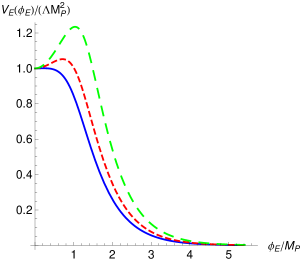
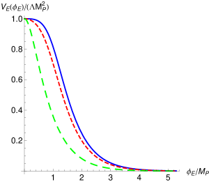
In figure 1 we show the effective potential in the Einstein frame as a function of the Einstein frame field for several values of and for fixed to . When both couplings are negative, the effective potential has one local maximum (at ) and it decays monotonically towards zero as the field increases (see left panel). However, when and , develops a local minimum at and two local maxima at some positive (right panel). In this paper we investigate the case when both couplings are negative and leave the latter case, in which tunneling from the local minimum can play an important role, for future work. While the field dependence of the potential in (5) is simple when expressed in terms of the Jordan frame field, there is no simple analytic form that describes the Einstein frame potential. This is a consequence of the fact that (4) cannot be solved analytically for . There are simple limits however. For small field values, , the potential in (5) can be approximated by a constant plus a negative mass term (as in hilltop inflation, see e.g. Refs. Boubekeur:2005zm ; Lyth:1998xn ),
| (6) |
while for , the potential decays exponentially with the field,
| (7) |
where is a constant whose value is . From Eqs. (6) and (7) we see that, if the field starts from some small value near the local maximum, it will slowly roll down the hill, exiting eventually inflation when .
One can show Glavan:2015ora that for , and in the Einstein frame
| (8) |
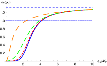
with the limiting value for . Here we have introduced quartic nonminimal coupling in in Eq. (2) in order to be able to relax the condition on and to still be able to terminate inflation. Namely, one can show that even when the quartic coupling is arbitrarily small and negative, will asymptotically reach the value , regardless of the value of negative . The condition during inflation requires which is satisfied by this setup.
One way of seeing this is to work in the adiabatic approximation and subsume the term in into a field dependent quadratic coupling as follows: . Now, when this is inserted into , which is the attractor value at asymptotically large field values, one obtains, for arbitrarily small, negative values of , see figure 2.
While inflation terminates when , is not enough to explain the post-inflationary radiation and matter eras. One can show Glavan:2015ora that a suitable coupling to a (perfect) matter fluid can induce the decay of into matter, such that in the tightly coupled regime, the system reaches . When matter is predominantly in the form of a relativistic fluid, for which the equation of state parameter , or equivalently , one will eventually reach a postinflationary radiation era, providing thus a graceful exit from inflation that is consistent with all observations.
III Slow roll inflation
We do not know what was the state of the Universe before inflation. It seems reasonable to assume that the Universe was expanding and that it was in a chaotic state, whose energy-momentum tensor was dominated by field fluctuations of various (energy and distance) scales. Even if not in equilibrium, such a state could be approximated by a nearly perfect fluid, whose equation of state is well approximated by the radiation equation of state, . In such a state nonminimal couplings do not play a significant role (since ), and thence it is natural to take the expectation value of the (quantum) field to be close to zero, .
As the Universe expands, the amplitude of fluctuations decreases, and the corresponding energy density and pressure decrease accordingly, reaching eventually the point when the contribution from the cosmological constant (whose origin may be both geometric and vacuum fluctuations of quantum fields) becomes significant. At that moment the Universe enters an inflationary phase, whereby the field feels a hilltop-like potential (6) and starts rolling down the hill. As it rolls, the contribution from fluctuations will rapidly redshift, becoming less and less important for the Universe’s dynamics. Thus we see that in our inflationary model the Universe enters inflation from a broad range of initial conditions without any need for (fine) tuning. Of course, it is still true that the cosmological constant and the nonminimal couplings have to have the right values (set by the COBE normalization of the amplitude of the scalar spectrum of cosmological perturbations and by the Planck value of the corresponding spectral slope). As we show below, these values can be obtained in our model by quite a natural choice of the parameters.
The Einstein frame action (5) implies the following equations of motion,
| (9) | |||||
| (10) | |||||
| (11) |
where the metric tensor is now, . While these equations can be solved numerically Glavan:2015ora without resorting to slow roll approximation (in which the Hubble parameter and possibly some of its time derivatives can be treated as adiabatic functions of time), it is instructive to use slow roll approximation because one can use analytical techniques that allow us to get a better grasp of the parameter dependencies of the observables. One can check the predictions of slow roll approximation by studying (approximate or exact) solutions of the attractor equation,
| (12) |
which is more general than slow roll approximation. This equation can be derived as follows. In general . However, it is often the case that the dependence on can be neglected because the initial conditions for are forgotten or is a function of (as it is, for example, in slow roll). More generally this will be the case when there is a phase space attractor towards which trajectories rapidly converge. 111An attractor behavior is opposite from a chaotic behavior, in which phase space trajectories repulse each other in the sense that they (exponentially) diverge from each other. In this case and Eq. (12) can be easily obtained by rewriting (11) as and inserting it into (10). With these caveats in mind, solving Eq. (12) is equivalent to solving the full system of equations (10–11) (Eq. (9) does not provide any new information as it can be obtained from the other two equations).
In slow roll approximation one neglects the first term in Eq. (9) and the kinetic term in Eq. (10) (the last equation is irrelevant because it is not independent). The memory of the initial conditions is neglected (because and are not independent variables and slow roll is an attractor). Moreover, the dependence on the initial field value is irrelevant, because one measures the number of e-folds from the end of inflation (at which the principal slow roll parameter ), and during inflation we are in the attractor. With these in mind, we can define the number of e-folds as,
| (13) | |||||
where we made use of,
| (14) |
Next, the principal slow roll parameter, reads in slow roll approximation,
| (15) |
The other two slow roll parameters can be defined in terms of the rate of change of as, , . In slow roll approximation they read,
| (16) |
The scalar and tensor perturbations are of the form,
| (17) |
where (to the leading order in slow roll approximation) the spectral indices and can be determined from the variation of and with respect to at the first horizon crossing during inflation (where ) as follows,
| (18) | |||||
| (19) |
Next, Eqs. (17) imply that the ratio of the tensor and scalar spectra is,
| (20) |
Finally, the running of the spectral index is,
| (21) |
This completes the calculation of the quantities required for slow roll analysis, which is used in the remainder of the paper. In our plots we shall sometimes express our quantities in terms of the Jordan frame field , and sometimes in terms of the number of e-folds in the Einstein frame, . For the latter it is useful to know how to calculate the field value at the end of inflation, which is by convention defined as the field value at which . A cursory look at Eq. (15) reveals that when , which is equivalent to the zeros of the following cubic equation for ,
| (22) |
Two of the zeros of this equation are complex and hence unphysical and one zero is real and positive, representing hence the unique physical solution defining the end of inflation. In the following analyzes we use that solution to signify the end of inflation.
An important question that needs to be addressed is the validity of slow roll approximation. When inflation lasts much longer than , it is to be expected that the field will be extremely close to the attractor regime described by Eq. (12). Under that assumption Eq. (12) can be used to test slow roll approximation. To get some insight into that question, we shall now study early time evolution of the field, which is described by Eq. (12). Inserting the Ansatz, into (12) yields a quadratic equation for ,
| (23) |
where we made use of , see Eq. (6). The two solutions are,
| (24) |
The physically relevant solution is the negative one, , as must decrease as increases. When , , so the leading order result in reproduces the slow roll result, and the higher order powers in are corrections to slow roll. Thus, as long as , the slow roll results should be trustable. This is, of course true, provided the attractor behavior (discussed above) is realised and does not depend on . At late times, when , the Einstein frame effective potential reduces to (7). It is well known that solutions to the Friedmann equations in such an exponential potential exhibit an attractor behavior Ratra:1987rm ; Joyce:1997fc ; Glavan:2015ora in which, while dominates the dynamics, , and asymptotically (when dominates), . The slow roll approximation again reproduces the leading order results: at intermediate times, , and at late times, , leading to an identical conclusion: as long as , slow roll approximation yields approximately correct results. With this in mind, we are ready to proceed to analyze our inflationary model in slow roll approximation. The analysis that goes beyond slow roll we leave for future work.
IV Results
In this section we present the principal results for the most important inflationary observables, which include: the amplitude of the scalar spectrum , scalar spectral index and its (logarithmic) running and the ratio of tensor and scalar perturbations, . We do not discuss separately the tensor spectral index and its running, but observe in passing that (within our approximations) the latter satisfies a consistency relation, and thus, up to a constant rescaling, is captured by the analysis of .
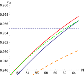
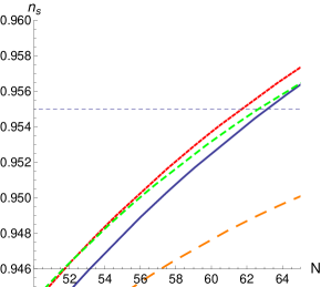
Figure 3 shows the dependence of the spectral index on the number of e-folds , taking and as parameters. The figure shows that peaks for (short red dashes), and it is very weakly dependent on (on the left panel and on the right panel ). Decreasing further would lead to smaller values of . Since the peak value of in our model is smaller (by about one standard deviation (dashed blue horizontal line)) than the central value of obtained by the Planck collaboration Ade:2015lrj , we conclude that our model gives the best results when preheating is instant and when and .
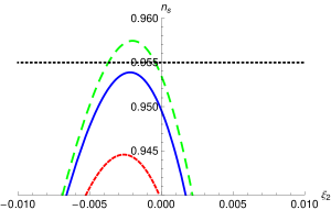
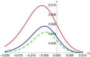
In figure 4 (left panel) we show the dependence of and on with the number of e-folds as a parameter (from bottom up: the curves corresponding to , and are shown). Figure 4 shows that the optimal value of is about , which is the value at which peaks. The peak value of is very weakly dependent on and decreases slowly as decreases. The right panel of figure 4 shows the ratio of the spectral amplitudes of tensor and scalar cosmological perturbations as a function of : is typically small and peaks for . Contrary to , shows a strong (approximately inversely proportional) dependence on , such that one can get as large as when .
Also from figure 4 one sees that the dependence of and on the number of e-folds (for a sufficiently large ) is approximately,
| (25) |
where is weakly dependent on and , and for the typical choice of the nonminimal couplings taken in this paper, . Likewise, is weakly dependent on and .
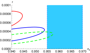
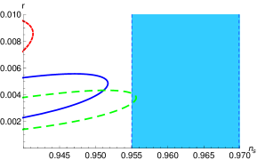
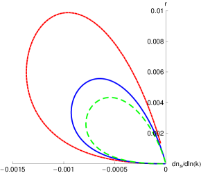
In figure 5 we show the ratio of the spectra of tensor and scalar cosmological perturbations as a function of the spectral index for the number of e-folds, (short red dashes), (blue solid) and (long green dashes). We see that the maximum value of increases as the number of e-folds increases, and it touches the lower observed bound on (taken from figure 4 of Ref. Ade:2015lrj , from where we took the contours obtained at the optimal value of the running spectral index) when . The question whether this high value of can be obtained within the standard cosmology (inflation followed by radiation and matter era) is discussed in the paragraph below. The model favors small values of . An that is large enough () to be observable by the near future planned missions (such as CORE+ and PRISM Andre:2013nfa ) can be obtained at the price of slightly decreasing , thus moving it further away (to about ) from the sweet spot, .
In conclusion, our analysis shows that, even though our model is
slightly (at ) disfavored by the current data, it is a
viable model of inflation.
A simple calculation shows that the number of e-folds during inflation that corresponds to some pivotal scale is (see e.g. Appendix B in Ref. Glavan:2014uga ),
| (26) |
where instant preheating is assumed. More accurately: an instant transition from inflation (during which ) to radiation (during which ) is assumed. In the above formula is the Hubble rate today, is the Hubble rate at the time when the pivotal comoving momentum exits the Hubble radius during inflation, is the comoving momentum corresponding to the Hubble scale today, and is the number of e-folds during matter era. Once is known, the number of e-folds during radiation era is easily calculated from . Taking during inflation gives – this result is correct provided stays constant during inflation and then relatively suddenly (within one or at most a few e-folds) changes at the end of inflation to . More realistically, changes gradually during inflation. Indeed, typical inflationary models predict , where is a constant of the order of unity. In these models needs to be replaced by its average value, . In this case Eq. (26) gives, . This is the maximum number of e-folds one can attain during inflation that correspond to the pivotal momentum in standard cosmology.
However, there are non-standard cosmologies Joyce:1997fc ; Joyce:2000ag ; Spokoiny:1993kt which include a period of kination (during which the kinetic energy of a scalar field dominates the energy density such that and ). During kination comoving modes approach the Hubble scale faster than during radiation or matter era, increasing thus the number of required inflationary e-folds. For example, when the number of e-folds of kination is of that in radiation, the number of e-folds (corresponding to ) increases from to .
In conclusion, a careful calculation shows that the number of
inflationary e-folds corresponding to the pivotal scale
used by the Planck collaboration is at
most (for standard cosmology), while in nonstandard
cosmologies (with e.g. a period of kination) it can be larger.
For these reasons in our figures we show results not just for
and , but also for .
Let us now try to figure out what the current data can tell us about the magnitude of the cosmological constant in our inflationary model. Recall that we know Ade:2015lrj that the amplitude of the scalar power spectrum (the COBE normalization) at the pivotal scale is . On the other hand, combining Eqs. (10), (17) and (20) gives,
| (27) |
where in the second equality we used the approximation, . To investigate whether the value of this cosmological constant is at the grand unified scale (GUT), let us define the GUT energy density as, , from which one gets,
| (28) |
Comparing this with (27) gives the following estimate of the grand unified scale producing ,
| (29) |
which yields when . Thus it is fair to say that for a rather broad range of ’s the cosmological constant in our model is at the grand unified scale.
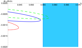
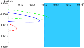
Figure 6 shows how the running of the spectral index depends on the spectral index . While the dependence of on and is by now familiar, we see from the figure that depends very weakly on (increasing slowly as increases), and for peaks at a value, , which is to be compared with the value observed by the Planck collaboration, Ade:2015lrj . Therefore, the spectral index running in our model is consistent with the current data and it is potentially observable provided the error bars decrease by about a factor of 10. It is unlikely that such an accuracy in can be attained by the near future CMB missions. Therefore, observing a running different from zero in the near future would be tantamount to ruling out our model.
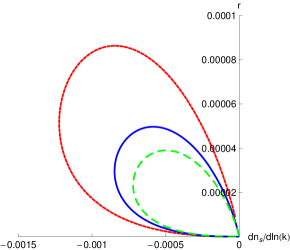
In figure 7 we show the dependence of on with as a parameter ( (short red dashes), (blue solid) and (long green dashed)). On the left panel , while on the right panel . The figure shows that, while the running very weakly dependents on , is approximately inversely proportional to . If future observations show that that would mean that would have to be small (e.g. ) and that would have to be below about .
V Discussion
In this paper we analyze a novel inflationary model, where inflation is driven by a (Jordan frame) cosmological constant and a nonminimally coupled scalar field plays the role of the inflaton. The model is inspired by the recent work Glavan:2015ora , where it was argued that, when viewed in the context of a nonminimally coupled scalar, a Jordan frame cosmological constant can be dynamically relaxed to zero (from the point of view of the Einstein frame observer). The model is analyzed in slow roll approximation, whose accuracy is (to a certain extent) tested. Our analysis shows that we can get the spectral index consistent with current observations, albeit the maximum value of the spectral index is about one standard deviation below the observed value, see figure 3. The value of the tensor-to-scalar ratio is typically small, see figure 4. Since is inversely proportional to the quartic nonminimal coupling , it can be enlarged by decreasing the value of to obtain an that is observable by the planned CMB experiments, but the price to pay is a smaller . The running of the spectral index is negative, see figures 6 and 7, but the typical amplitude of the running is by about one order of magnitude below the sensitivity of the current CMB data.
It is worth noting that the value of the cosmological constant is to a large extent determined by the COBE normalization and it is of the order of the GUT scale, i.e. , and hence it can be nicely attributed to the value attained at a GUT transition (both from the Higgs potential as well as from the contributions generated by the particle masses). A second nice feature of the model at hand is that the model works for a large class of initial conditions. Namely, inflation naturally begins from a chaotic state, in which the total (averaged) energy in fluctuations scales as and during which the average field value is naturally small, (this is so because the nonminimal coupling plays no role as the Ricci scalar is small, ). Sometime after the GUT transition the cosmological constant starts dominating the energy density, and one enters (slow roll) inflation. Inflation is terminated as ; at asymptotically late times . Graceful exit and preheating is solved by suitably coupling the scalar field to matter, for details see Ref. Glavan:2015ora . Another advantage of our model is in that there is no need to fine tune the potential to zero at the end of inflation, thus getting rid of one of the major fine tuning problems of scalar inflationary models.
From our analysis it is not completely clear how accurate is the slow roll approximation utilized in this paper. For that reason we are working on studying predictions of the inflationary model presented here by using exact solutions of the Friedmann equations (9–11). One hope is that, performing an exact analysis will allow us to obtain values for and that are closer to the (central) values favored by current observations, and thus get an even better agreement with the data.
Acknowledgements
This work is part of the D-ITP consortium, a program of the Netherlands Organization for Scientific Research (NWO) that is funded by the Dutch Ministry of Education, Culture and Science (OCW). A.M. is funded by NEWFELPRO, an International Fellowship Mobility Programme for Experienced Researchers in Croatia and by the D-ITP.
References
- (1) P. Jordan, “Schwerkraft und Weltall,” Friedrich Vieweg and Sohn, Braunschweig (1955).
- (2) C. Brans and R. H. Dicke, “Mach’s principle and a relativistic theory of gravitation,” Phys. Rev. 124 (1961) 925.
- (3) P. G. Bergmann, “Comments on the scalar tensor theory,” Int. J. Theor. Phys. 1 (1968) 25.
- (4) R. Fakir and W. G. Unruh, “Improvement on cosmological chaotic inflation through nonminimal coupling,” Phys. Rev. D 41 (1990) 1783.
- (5) D. S. Salopek, J. R. Bond and J. M. Bardeen, “Designing Density Fluctuation Spectra in Inflation,” Phys. Rev. D 40 (1989) 1753.
- (6) F. L. Bezrukov and M. Shaposhnikov, “The Standard Model Higgs boson as the inflaton,” Phys. Lett. B 659 (2008) 703 [arXiv:0710.3755 [hep-th]].
- (7) F. Bezrukov, “The Higgs field as an inflaton,” Class. Quant. Grav. 30 (2013) 214001 [arXiv:1307.0708 [hep-ph]].
- (8) T. Prokopec and J. Weenink, “Naturalness in Higgs inflation in a frame independent formalism,” arXiv:1403.3219 [astro-ph.CO].
- (9) A. D. Dolgov, “An Attempt To Get Rid Of The Cosmological Constant,” In *Cambridge 1982, Proceedings, The Very Early Universe*, 449-458
- (10) L. H. Ford, “Cosmological Constant Damping By Unstable Scalar Fields,” Phys. Rev. D 35 (1987) 2339.
- (11) S. Weinberg, “The Cosmological Constant Problem,” Rev. Mod. Phys. 61 (1989) 1.
- (12) D. Glavan and T. Prokopec, “Nonminimal coupling and the cosmological constant problem,” arXiv:1504.00842 [gr-qc].
- (13) D. Glavan, T. Prokopec and D. C. van der Woude, “Late-time quantum backreaction from inflationary fluctuations of a nonminimally coupled massless scalar,” Phys. Rev. D 91 (2015) 2, 024014 [arXiv:1408.4705 [gr-qc]].
- (14) D. Glavan, T.Prokopec and A. Starobinsky, in progress (2015); D. Glavan, T.Prokopec and T. Takahashi, in progress.
- (15) E. J. Copeland, M. Sami and S. Tsujikawa, “Dynamics of dark energy,” Int. J. Mod. Phys. D 15 (2006) 1753 [hep-th/0603057].
- (16) P. J. E. Peebles and B. Ratra, “The Cosmological constant and dark energy,” Rev. Mod. Phys. 75 (2003) 559 [astro-ph/0207347].
- (17) C. M. Will, “The Confrontation between general relativity and experiment,” Living Rev. Rel. 9 (2006) 3 [gr-qc/0510072].
- (18) J. Weenink and T. Prokopec, “Gauge invariant cosmological perturbations for the nonminimally coupled inflaton field,” Phys. Rev. D 82 (2010) 123510 [arXiv:1007.2133 [hep-th]].
- (19) T. Prokopec and J. Weenink, “Frame independent cosmological perturbations,” JCAP 1309 (2013) 027 [arXiv:1304.6737 [gr-qc]].
- (20) T. Prokopec and J. Weenink, “Uniqueness of the gauge invariant action for cosmological perturbations,” JCAP 1212 (2012) 031 [arXiv:1209.1701 [gr-qc]].
- (21) D. H. Lyth and A. Riotto, “Particle physics models of inflation and the cosmological density perturbation,” Phys. Rept. 314 (1999) 1 [hep-ph/9807278].
- (22) L. Boubekeur and D. H. Lyth, “Hilltop inflation,” JCAP 0507 (2005) 010 [hep-ph/0502047].
- (23) M. Joyce and T. Prokopec, “Turning around the sphaleron bound: Electroweak baryogenesis in an alternative postinflationary cosmology,” Phys. Rev. D 57 (1998) 6022 [hep-ph/9709320].
- (24) B. Ratra and P. J. E. Peebles, “Cosmological Consequences of a Rolling Homogeneous Scalar Field,” Phys. Rev. D 37 (1988) 3406.
- (25) P. A. R. Ade et al. [Planck Collaboration], “Planck 2015 results. XX. Constraints on inflation,” arXiv:1502.02114 [astro-ph.CO].
- (26) P. Andr et al. [PRISM Collaboration], “PRISM (Polarized Radiation Imaging and Spectroscopy Mission): An Extended White Paper,” JCAP 1402 (2014) 006 [arXiv:1310.1554 [astro-ph.CO]].
- (27) B. Spokoiny, “Deflationary universe scenario,” Phys. Lett. B 315 (1993) 40 [gr-qc/9306008].
- (28) M. Joyce and T. Prokopec, “Baryogenesis from ‘electrogenesis’ in a scalar field dominated epoch,” JHEP 0010 (2000) 030 [hep-ph/0003190].