Spatio-angular Minimum-variance Tomographic Controller for Multi-Object Adaptive Optics systems

Abstract

Multi-object astronomical adaptive-optics (MOAO) is now a mature wide-field observation mode to enlarge the adaptive-optics-corrected field in a few specific locations over tens of arc-minutes.

The work-scope provided by open-loop tomography and pupil conjugation is amenable to a spatio-angular Linear-Quadratic Gaussian (SA-LQG) formulation aiming to provide enhanced correction across the field with improved performance over static reconstruction methods and less stringent computational complexity scaling laws.

Starting from our previous work correia14 , we use stochastic time-progression models coupled to approximate sparse measurement operators to outline a suitable SA-LQG formulation capable of delivering near optimal correction. Under the spatio-angular framework the wave-fronts are never explicitly estimated in the volume, providing considerable computational savings on 10 m-class telescopes and beyond.

We find that for Raven, a 10m-class MOAO system with two science channels, the SA-LQG improves the limiting magnitude by two stellar magnitudes when both Strehl-ratio and Ensquared-energy are used as figures of merit. The sky-coverage is therefore improved by a factor of $\sim$5.

I Intro: Multi-object adaptive optics systems

Multi-object Adaptive Optics (MOAO) is now a well-established AO concept to enlarge the corrected field to several arcminutes when only a few directions of interest exist in the field and need be corrected for vidal10 ; andersen12 ; correia14 ; sivo14 .

Similarly to multi-conjugate AO (MCAO) it relies on tomography to provide a tridimensional wave-front estimation above the telescope and thereupon provide correction on several scientific relevant directions, reaching out for a multiplexing factor of up to 20 on ELT-sized systems andersen06 ; hammer14 .

On a previous paper correia14 we have outlined the static minimum-mean square error (MMSE) spatio-angular (SA) wave-front estimation (time-dependent wave-front evolution not considered) when a Zernike polynomial basis is used and suggested predictive models to overcome temporal lag errors when aiming for increased sky-coverage jackson15 . In the SA case estimating the tomographic phase explicitly is circumvented, only the aperture-plane is estimated to be later least-squares fitted onto the DM – the Learn&Apply approach in vidal10 is similar albeit in a different vector space.

We now move one step forward: we provide extensions to use a zonal basis set coupled to the optimal minimum residual phase error variance Linear-Quadratic-Gaussian (LQG) controller tailored to MOAO systems.The LQG controller has been presented in the AO context in several works piatrou05 ; correia10a ; gilles13 ; sivo14 and here it is designed and optimized for a MOAO system performing open-loop tomography and single-layer optical conjugation. We further propose a minimal state representation together with first-order near-Markovian predictive models which lead to a computational complexity of the order of the static MMSE reconstructors for a multiplexing capability of 20 science targets.

The use of a spatio-angular framework has several advantages over the formulation that estimates the layered phase explicitly:

1. the real-time computation is independent from the number of atmospheric layers;

2. the analytical spatio-angular covariance matrices can be computed explicitly thus avoiding interpolation through the ray-tracing operation to obtain the integrated pupil-plane wave-front profile;

3. in principle a hybrid data-driven model-based controller can be designed since a subset of the covariance matrices can be acquired directly from the system (i.e. empirically acquired) instead of relying fully on models; alternatively meta-parameters can be identified from which enhanced models are obtained.

4. the sparseness of the LQG compounding matrices can still, albeit to a lesser degree, be exploited for real-time savings as noted in jackson15 ; correia09 .

The goal of this paper is therefore two-fold:

i) fully outline the zonal LQG minium-variance tomographic controller design to optimize optical performance, particularly in poor signal-to-noise ratio regimes such that sky-coverage can be improved upon by guiding on fainter sources and

ii) provide a suitable, Extremely Large Telescope (ELT)-compliant spatio-angular formulation for the Kalman estimator (and static MMSE) that decouples the wave-front reconstruction from the number of atmospheric layers used to model it.

We present results from both simulation and the optical bench of the Raven system, a MOAO science and technology demonstrator installed on the 8 m Subaru telescope andersen12 .

This paper is organized as follows. Section 2 outlines the LQG formulation, section 3 discusses other SA implementations, namely the static SA reconstructors obtained from the LQG, section 4 provides sample numerical results whereas section 5 overviews the Raven optical bench and the results obtained in the lab. Section 6 provides the summary and conclusions.

II Spatio-angular LQG formulation

II.1 Definitions and assumptions

We define the pupil-plane wave-front ${\boldsymbol{\psi}}(\boldsymbol{\rho},{\boldsymbol{\theta}},t)$ indexed by the bi-dimensional spatial coordinate vector $\boldsymbol{\rho}=[\rho_{x},\rho_{y}]$ in direction ${\boldsymbol{\theta}}=[\theta_{x},\theta_{y}]$ at time $t$ under the hypothesis that the turbulent atmosphere is a sum of $L$ thin layers located in a discrete number of different altitudes $h_{l}$ as

$${\boldsymbol{\psi}}(\boldsymbol{\rho},{\boldsymbol{\theta}},t)=[\mathbf{H}{\boldsymbol{\varphi}}](\boldsymbol{\rho},t)=\sum_{l=1}^{L}\omega_{l}{\boldsymbol{\varphi}}_{l}(\boldsymbol{\rho}+h_{l}{\boldsymbol{\theta}},t)$$ (1)

where ${\boldsymbol{\varphi}}_{l}(\boldsymbol{\rho},t)$ is the $l^{th}$-layer wave-front, $\omega_{l}$ is the $l^{th}$ layer relative strength and $\mathbf{H}$ is a geometric optics propagation operator in the near-field approximation (commonly called ray-tracing gilles02 ) that relates the aperture-plane wave-front (WF) to the layered wave-fronts by adding and interpolating ${\boldsymbol{\varphi}}_{l}(\boldsymbol{\rho}+h_{l}{\boldsymbol{\theta}},t)$ on the aperture-plane ($h_{0}=0$) computational grid ellerbroek02a .

In the following we assume the frozen-flow hypothesis whereby ${\boldsymbol{\varphi}}(\boldsymbol{\rho},t+\tau)={\boldsymbol{\varphi}}(\boldsymbol{\rho}-\mathbf{v}\tau,t)$ with $\mathbf{v}=[v_{x};v_{y}]$ the wind velocity vector. A discrete-time, point-wise representation of the WF is also assumed throughout this paper.

We further assume that averaged phase values over the wave-front sensor (WFS) integration period $T_{s}$ are taken at face value, i.e

$${\boldsymbol{\varphi}}_{k}(\boldsymbol{\rho})=\frac{1}{T_{s}}\int_{(k-1)T_{s}}^{kT_{s}}{\boldsymbol{\varphi}}(\boldsymbol{\rho},t)\,\mathrm{d}t,$$ (2)

and that the commands are piece-wise constant over an entire frame (either synchronous or not with the WFS sampling frames)

$${\mathbf{u}}_{k}\triangleq{\mathbf{u}}(t),\,\,\,\,kT_{s}\leq t<(k+1)T_{s}$$ (3)

Ensemble averaging is represented by $\left\langle{\cdot}\right\rangle$ with shorthand covariance matrix notation $\boldsymbol{\Sigma}_{u,v}=\left\langle{uv^{\mathsf{T}}}\right\rangle$. Angles are notated in general ${\boldsymbol{\theta}}$ and guide-star and science directions use ${\boldsymbol{\alpha}}$ and ${\boldsymbol{\beta}}$ respectively.

II.2 LQG regulator synthesis

The derivation of the LQG for AO applications has been presented in detail elsewhere for either the infinitely fast DM response or otherwise correia10a . In this paper we therefore take a shorter path for the sake of conciseness and refer the reader to the bibliographic references on this particular subject for a more in-depth derivation.

The discrete-time LQG regulator minimizes the cost function

$$J({\mathbf{u}}) =\lim_{M\rightarrow\infty}\frac{1}{M}\sum_{k=0}^{M-1}\left({\mathbf{x}}^{\mathsf{T}}\mathbf{Q}{\mathbf{x}}+{\mathbf{u}}^{\mathsf{T}}\mathbf{R}{\mathbf{u}}+2{\mathbf{x}}^{\mathsf{T}}\mathbf{S}{\mathbf{u}}\right)_{k}$$ (4)

where the weighting triplet $\{\mathbf{Q},\mathbf{R},\mathbf{S}\}$ is made apparent and will be specified next by developing a MOAO-specific quadratic criterion subject to the state-space model

$$\left\{\begin{array}[]{ccl}{\mathbf{x}}_{k+1}&=&\mathcal{A}{\mathbf{x}}_{k}+\mathcal{B}{\mathbf{u}}_{k}+\mathcal{V}\boldsymbol{\nu}_{k}\\ {\mathbf{s}}_{{\boldsymbol{\alpha}},k}&=&\mathcal{C}{\mathbf{x}}_{k}+\mathcal{D}{\mathbf{u}}_{k}+{\boldsymbol{\eta}}_{k}\end{array}\right.$$ (5)

where ${\mathbf{x}}_{k}$ is the state vector that contains if not the phase directly a linear combination thereof, ${\mathbf{s}}_{{\boldsymbol{\alpha}},k}$ are the noisy measurements provided by the WFS in the GS directions, $\boldsymbol{\nu}_{k}$ and ${\boldsymbol{\eta}}_{k}$ are spectrally white, Gaussian-distributed state excitation and measurement noise respectively. In the following we assume that $\boldsymbol{\Sigma}_{\boldsymbol{\nu}}=\left\langle{\boldsymbol{\nu}\boldsymbol{\nu}^{\mathsf{T}}}\right\rangle$, $\boldsymbol{\Sigma}_{\mathbf{\boldsymbol{\eta}}}=\left\langle{\boldsymbol{\eta}\boldsymbol{\eta}^{\mathsf{T}}}\right\rangle$ are known and that $\boldsymbol{\Sigma}_{\mathbf{\boldsymbol{\eta,\nu}}}=\left\langle{\boldsymbol{\eta}\boldsymbol{\nu}^{\mathsf{T}}}\right\rangle=0$.

II.3 Minimum residual phase variance after correction

The objective cost function considered for MOAO is the minimisation of the aperture-plane residual phase variance for individual science directions ${\boldsymbol{\beta}}_{i}\in\Re^{1\times 2}$ leading to the maximisation of the Strehl-ratio.

If we denote the term $\boldsymbol{\epsilon}_{k}\triangleq{{\boldsymbol{\psi}}}(\boldsymbol{\rho},{\beta_{i}},kT_{s})-{{\boldsymbol{\psi}}}^{\mathsf{\tiny{cor}}}(\boldsymbol{\rho},{\beta_{i}},kT_{s})$ the residual phase profile after DM correction with ${{\boldsymbol{\psi}}}(\boldsymbol{\rho},{\beta_{i}},kT_{s})=\mathbf{H}_{\beta_{i}}{{\boldsymbol{\varphi}}}(\boldsymbol{\rho},kT_{s})$ the aperture-plane wave-front in a particular direction in the field and $-{{\boldsymbol{\psi}}}^{\mathsf{\tiny{cor}}}(\boldsymbol{\rho},{\beta_{i}},kT_{s})$ the DM-produced correction phase in that direction, the mean square residual piston-removed wave-front error over the telescope aperture is $\sigma^{2}_{k}=\|\boldsymbol{\epsilon}_{k}\|^{2}_{W,L_{2}(\Omega)}=\boldsymbol{\epsilon}_{k}^{\mathsf{T}}W\boldsymbol{\epsilon}_{k}$ where $W$ is a positive-definite weighting matrix that removes the piston contribution over the telescope aperture ellerbroek02 and $L_{2}$ is the Euclidean norm over the aperture $\Omega$.

The integration, reading, processing and correction in the AO loop are done in discrete-time leading to intrinsic lags which take customarily several milliseconds. We will expand the discussion of time delays for synchronous and asynchronous systems in §II.5.

Using the definitions of integrated phase and commands in §II.1 we can now ascertain the discrete-time minimum residual phase variance (MV) criterion

$$J({\mathbf{u}}) =\lim_{M\rightarrow\infty}\frac{1}{M}\sum_{k=0}^{M-1}\sigma^{2}_{k}$$

$$=\lim_{M\rightarrow\infty}\frac{1}{M}\sum_{k=0}^{M-1}\|{\boldsymbol{\psi}}_{k+1}(\boldsymbol{\rho},{\boldsymbol{\beta}})-\mathbf{N}{\mathbf{u}}_{k}(\boldsymbol{\rho},{\boldsymbol{\beta}})\|^{2}_{W,L_{2}(\Omega)}$$ (6)

which neglects any WF dynamics during the integration. The error that is neglected here has been dubbed insurmountable error due to the use of averaged variables instead of continuous ones correia10a and is negligible for the most common systems operating at high frame-rates.

Provided the phase vector ${{\boldsymbol{\psi}}}_{k+1}$ is known the solution to Eq. (II.3) is straightforwardly shown to be a least-squares fit onto the DM influence functions kulcsar06 ; correia10a

$${\mathbf{u}}_{k}(\boldsymbol{\rho},{\boldsymbol{\beta}}) =\mathbf{F}{{\boldsymbol{\psi}}}_{k+1}(\boldsymbol{\rho},{\boldsymbol{\beta}})$$

$$=(\mathbf{N}^{\mathsf{T}}W\mathbf{N})^{-1}\mathbf{N}^{\mathsf{T}}W{\boldsymbol{\psi}}_{k+1}(\boldsymbol{\rho},{\boldsymbol{\beta}})$$ (7)

The latter would have been likewise found from the degenerate control Riccati equation, whose discussion we avert here but can be found for instance in kulcsar12 ; correia10a .

We now deal with the general case where ${\boldsymbol{\psi}}_{k+1}$ is not known in Eq. (II.3) but needs be estimated from linearly related noisy measurements.

The separation principle andersonmoore_optimalcontrolLQG05 provides immediately the solution

$${\mathbf{u}}_{k}(\boldsymbol{\rho},{\boldsymbol{\beta}}) =\mathbf{F}\widehat{{\boldsymbol{\psi}}}_{k+1|k}(\boldsymbol{\rho},{\boldsymbol{\beta}})$$

$$=(\mathbf{N}^{\mathsf{T}}W\mathbf{N})^{-1}\mathbf{N}^{\mathsf{T}}W\widehat{{\boldsymbol{\psi}}}_{k+1|k}(\boldsymbol{\rho},{\boldsymbol{\beta}}),$$ (8)

where $\widehat{{\boldsymbol{\psi}}}_{k+1|k}(\boldsymbol{\rho},{\boldsymbol{\beta}})=\widehat{{\boldsymbol{\psi}}}_{k+1|\mathcal{S}_{k}({\boldsymbol{\alpha}})}(\boldsymbol{\rho},{\boldsymbol{\beta}})=E({{\boldsymbol{\psi}}}_{k+1}(\boldsymbol{\rho},{\boldsymbol{\beta}})|\mathcal{S}_{k}(\boldsymbol{\rho},{\boldsymbol{\alpha}}))$ is the conditional expectation of ${{\boldsymbol{\psi}}}_{k+1}({\boldsymbol{\beta}})$ in the science directions with respect to the sequence of all measurements from (in general non-coincidental) GS directions available up to $t=kT_{s}$, i.e. $\mathcal{S}_{k}=\{{\mathbf{s}}_{0},\cdots,{\mathbf{s}}_{k}\}(\boldsymbol{\rho},{\boldsymbol{\alpha}})$ andersonmoore_optimalfiltering05 . This conditional expectation is readily available from a Kalman filter andersonmoore_optimalcontrolLQG05 ; correia10a ; gilles13 . It relies on the definition of the first-differences state-space model in Eq. (5) whose construction is shown further below.

II.3.1 near-Markovian time-progression model of the 1st-order

The use of auto-regressive models has been given wide attention using the Zernike polynomials’ expansion basis set petit09 ; sivo14 as well as with Fourier modes for which a complex model encodes perfectly spatial shifts and thus frozen-flow poyneer08 .

We restrict our attention to the near-Markovian first-order time-evolution model gavel02a which has delivered best overall performance albeit with increased computational complexity piatrou07 ; correia14 ; jackson15 (spatial dependence omitted)

$${\boldsymbol{\psi}}_{k+\Delta}({\boldsymbol{\alpha}})={\mathbf{A}}{\boldsymbol{\psi}}_{k}({\boldsymbol{\alpha}})+\boldsymbol{\nu}_{k}({\boldsymbol{\alpha}})$$ (9)

with $\Delta=\tau/T_{s}$ is a delay in units of sample step $T_{s}$, where the transition matrix minimizes the quadratic criterion correia14

$${\mathbf{A}}=\arg\min_{{\mathbf{A}}^{\prime}}\left\langle{\left\|{\boldsymbol{\psi}}_{k+\Delta}({\boldsymbol{\alpha}})-{\mathbf{A}}^{\prime}{\boldsymbol{\psi}}_{k}({\boldsymbol{\alpha}})\right\|^{2}_{L_{2}(\Omega)}}\right\rangle,$$ (10)

The solution to Eq. (10) is

$${\mathbf{A}}=\left\langle{{\boldsymbol{\psi}}_{k+\Delta}{\boldsymbol{\psi}}_{k}^{\mathsf{T}}}\right\rangle\left\langle{{\boldsymbol{\psi}}_{k}{\boldsymbol{\psi}}_{k}^{\mathsf{T}}}\right\rangle^{-1}({\boldsymbol{\alpha}})$$ (11)

Note that we do not remove piston in this equation although we could following formulae in wallner83 .

By denoting ${\boldsymbol{\psi}}_{k}(\boldsymbol{\rho},{\boldsymbol{\alpha}})=\mathbf{H}_{\boldsymbol{\alpha}}{\boldsymbol{\varphi}}(\boldsymbol{\rho},kT_{s})$ and substituting in Eq. (11) we get

$${\mathbf{A}} =\mathbf{H}_{\boldsymbol{\alpha}}\left\langle{{\boldsymbol{\varphi}}_{k+\Delta}{\boldsymbol{\varphi}}_{k}^{\mathsf{T}}}\right\rangle\left\langle{{\boldsymbol{\varphi}}_{k}{\boldsymbol{\varphi}}_{k}^{\mathsf{T}}}\right\rangle^{-1}\mathbf{H}_{\boldsymbol{\alpha}}^{{\dagger}}$$ (12)

$$=\mathbf{H}_{\boldsymbol{\alpha}}\left\langle{{\boldsymbol{\varphi}}(\boldsymbol{\rho}-\mathbf{v}\tau){\boldsymbol{\varphi}}(\boldsymbol{\rho})^{\mathsf{T}}}\right\rangle\left\langle{{\boldsymbol{\varphi}}(\boldsymbol{\rho}){\boldsymbol{\varphi}}(\boldsymbol{\rho})^{\mathsf{T}}}\right\rangle^{-1}\mathbf{H}_{\boldsymbol{\alpha}}^{{\dagger}}$$

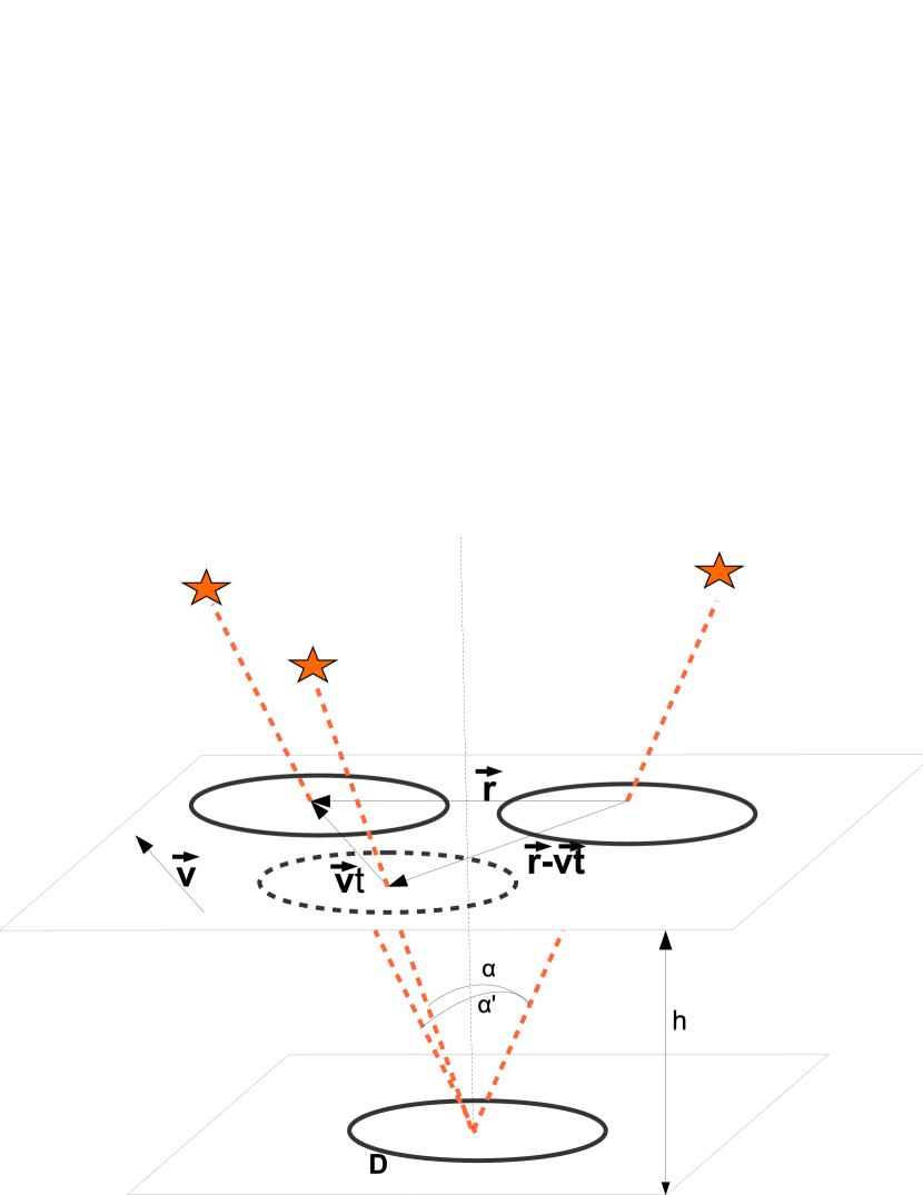
where ${\boldsymbol{\psi}}_{k+\Delta}(\boldsymbol{\rho},{\boldsymbol{\alpha}})=\mathbf{H}_{\boldsymbol{\alpha}}{\boldsymbol{\varphi}}(\boldsymbol{\rho}-\mathbf{v}\tau kT_{s})=\mathbf{H}_{{\boldsymbol{\alpha}}^{\prime}}{\boldsymbol{\varphi}}(\boldsymbol{\rho},kT_{s})$ which translates the spatio-angular nature of the computation we are accomplishing since a time-translation is factored in as an altitude-dependent angular shift using the frozen-flow hypothesis. Figure 1 shows pictorially the statements made.

Figure 1: Spatio-angular computation scheme. Pupil displacements are highly exaggerated for viewing. The spatio-angular correlations are computed with the pupil located at $\boldsymbol{\rho}-{\mathbf{v}}\tau$ where $\tau$ is time in seconds.

Assuming stationarity, the state excitation noise covariance matrix is found for a first order time-evolution model from the covariance equality (implicit indices dropped out)

$$\left\langle{{\boldsymbol{\psi}}{\boldsymbol{\psi}}^{\mathsf{T}}}\right\rangle={\mathbf{A}}\left\langle{{\boldsymbol{\psi}}{\boldsymbol{\psi}}^{\mathsf{T}}}\right\rangle{\mathbf{A}}^{\mathsf{T}}+\left\langle{\boldsymbol{\nu}\boldsymbol{\nu}^{\mathsf{T}}}\right\rangle,$$ (13)

since $\left\langle{{\boldsymbol{\psi}}_{k+1}{\boldsymbol{\psi}}_{k+1}^{\mathsf{T}}}\right\rangle=\left\langle{{\boldsymbol{\psi}}_{k}{\boldsymbol{\psi}}_{k}^{\mathsf{T}}}\right\rangle=\left\langle{{\boldsymbol{\psi}}{\boldsymbol{\psi}}^{\mathsf{T}}}\right\rangle$. The excitation noise covariance matrix is therefore

$$\left\langle{\boldsymbol{\nu}\boldsymbol{\nu}^{\mathsf{T}}}\right\rangle=\left\langle{{\boldsymbol{\psi}}{\boldsymbol{\psi}}^{\mathsf{T}}}\right\rangle-{\mathbf{A}}\left\langle{{\boldsymbol{\psi}}{\boldsymbol{\psi}}^{\mathsf{T}}}\right\rangle{\mathbf{A}}^{\mathsf{T}}$$ (14)

The model driving noise covariance matrix $\left\langle{\boldsymbol{\nu}\boldsymbol{\nu}^{\mathsf{T}}}\right\rangle$ is a key element of the KF design.

II.3.2 Measurement model

The presentation that now takes place restricts itself to the case of the Shack-Hartmann (SH) WFS which provides the averaged phase gradient over a regular grid of sub-apertures in the pupil-plane hardy98 .

We use a geometrical linear model which we assume valid for the regime of operation it will be submitted to; the model is thus

$${\mathbf{s}}_{k}({\boldsymbol{\alpha}})=\mathbf{G}{\boldsymbol{\psi}}_{k}({\boldsymbol{\alpha}})+{\boldsymbol{\eta}}_{k}({\boldsymbol{\alpha}})$$ (15)

where ${\boldsymbol{\eta}}_{k}$ represents photon an detector shot noise taken to be additive Gaussian noise of know covariance and $\mathbf{G}$ is a matrix whose entries are computed from the discretization of the wave-front gradients in the ${{N_{\alpha}}}$ GS directions. It uses a 3x3 regular stencil to compute the averaged phase gradient with Simpson weights for the fully-illuminated sub-apertures

$$w_{x}=\frac{1}{d}\left[\begin{array}[]{ccc}-1/4&0&1/4\\ -1/2&0&1/2\\ -1/4&0&1/4\end{array}\right],w_{y}=-w_{x}^{\mathsf{T}}$$ (16)

The stencils for partially illuminated sub-apertures at the outer and inner edge of the telescope pupil are found by expanding the phase on a set of bilinear splines and computing the average gradient over each of the four quadrant patches. The derivation of this result is out of scope but can be found at request in waddle12 .

This sampling and respective estimation of wave-fronts at twice the SH-WFS’s Nyquist frequency permits the rejection of some aliasing that affects the original measurements as outlined in petit09 . An enhanced model with coloured noise is shown in poyneer10 .

Note that in our implementation we will not make explicit use of the ray tracing $\mathbf{H}$ in Eq. (15) since the layered phase need not be estimated – no multi-conjugation step ensues. Only the pupil-plane phase is of interest which opens up to considerable modelling simplifications using a spatio-angular frame-work.

This is a fundamental simplification with respect to previous tomographic LQG implementations – which in the remainder is called E-LQG to account for the explicit estimation step. We avoid estimating the layered wave-front as is customarily done, focusing in estimating the integrated pupil-plane wave-fronts in the GS directions along their lines of sight. The angular anisoplanatic estimate is made on a subsequent step by invoking linearity, stationarity and Gaussianity as in the static case correia14 .

II.4 Minimal state-space representation: compactness in Open-Loop AO

The combination of enhanced spatio-angular first-order predictive models with single-conjugate correction allows for some modelling simplifications that in turn will make for smaller problem size and less stringent real-time and off-line computational requirements.

Under these working assumptions, the LQG model admits – unlike previous implementations piatrou07 ; sivo14 – a minimal state representation with phase taken at one single time instant. To do so one assumes the measurements are available at the end of the WFS integration step, regardless of the actual temporal delay in the system correia10a : one affects thus the whole delay to the commands instead of the measurements.

On top of this, we can further use a state vector with the pupil-plane phase integrated over directions ${\boldsymbol{\alpha}}\in[1,\cdots,N_{\alpha}]$ at instant $k$ to provide the Spatio-Angular LQG formulation.

Selecting thus ${\mathbf{x}}_{k}\triangleq{\boldsymbol{\psi}}_{k}({\boldsymbol{\alpha}})$

$${\boldsymbol{\psi}}_{k}({\boldsymbol{\alpha}})=\left(\begin{array}[]{c}{\boldsymbol{\psi}}({{\boldsymbol{\alpha}}_{1}})\\ \cdots\\ {\boldsymbol{\psi}}({{\boldsymbol{\alpha}}_{N_{\alpha}}})\end{array}\right)_{k}$$ (17)

where the state is a concatenation of phase vector in the $N_{\alpha}$ guide-star directions, one defines the state space terms for Eq. (9)

$$\left[\begin{array}[]{c|c|c}\mathcal{A}&\mathcal{B}&\mathcal{V}\\ \hline\cr\mathcal{C}&\mathcal{D}&\mathsf{0}\end{array}\right]=\left[\begin{array}[]{c|c|c}{\mathbf{A}}&\mathsf{0}&\mathbf{I}\\ \hline\cr\mathbf{G}&\mathsf{0}&\mathsf{0}\end{array}\right]$$ (18)

The implementation of the KF involves a real-time state update and prediction equations which in the SA case are

$$\widehat{{\boldsymbol{\psi}}}_{k|k}({\boldsymbol{\alpha}}) =\widehat{{\boldsymbol{\psi}}}_{k|k-1}({\boldsymbol{\alpha}})+\mathcal{H}_{\infty}\left({\mathbf{s}}_{k}({\boldsymbol{\alpha}})-\mathbf{G}\widehat{{\boldsymbol{\psi}}}_{k|k-1}({\boldsymbol{\alpha}})\right)$$ (19a)

$$\widehat{{\boldsymbol{\psi}}}_{k+1|k}({\boldsymbol{\alpha}}) ={\mathbf{A}}\widehat{{\boldsymbol{\psi}}}_{k|k}({\boldsymbol{\alpha}})$$ (19b)

where $\mathcal{H}_{\infty}$ is the asymptotic Kalman gain computed from the solution of an estimation Riccati equation correia10a . The use of the asymptotic value is justified, like elsewhere petit08 for one seeks long-exposure performance therefore employing the steady-state gain with no loss of performance. Whenever implicit we drop the notation $({\boldsymbol{\alpha}})$.

Under the choice of state made earlier, the $L_{2}$ criterion in Eq. (II.3) assumes the equivalent form

$$J({\mathbf{u}})= \lim_{M\rightarrow\infty}$$

$$\frac{1}{M}\sum_{k=0}^{M-1}\left(\begin{array}[]{c}{\mathbf{x}}_{k}\\ {\mathbf{u}}_{k}\end{array}\right)^{\mathsf{T}}\left(\begin{array}[]{cc}{\mathbf{A}}^{\mathsf{T}}{\mathbf{A}}&-{\mathbf{A}}^{\mathsf{T}}\mathbf{N}\\ -\mathbf{N}^{\mathsf{T}}{\mathbf{A}}&\mathbf{N}^{\mathsf{T}}\mathbf{N}\end{array}\right)\left(\begin{array}[]{c}{\mathbf{x}}_{k}\\ {\mathbf{u}}_{k}\end{array}\right)$$ (26)

from which $\mathbf{Q}={\mathbf{A}}^{\mathsf{T}}{\mathbf{A}}\geq\mathbf{0}$, $\mathbf{R}=\mathbf{N}^{\mathsf{T}}\mathbf{N}>\mathbf{0}$ and $\mathbf{S}=-{\mathbf{A}}^{\mathsf{T}}\mathbf{N}$; this construction ensures a stable controller since ${\mathbf{A}}$ is a positive definite stability matrix with $|eig({\mathbf{A}})|<1$ and $\mathbf{Q}-\mathbf{S}\mathbf{R}\mathbf{S}^{\mathsf{T}}\geq 0$ and $\mathbf{R}$ a full-rank matrix.

II.5 Time-delayed correction: synchronous and asynchronous commands

From phase estimates $\widehat{{\boldsymbol{\psi}}}_{k|k}({\boldsymbol{\alpha}})$ any future disturbance can be computed using the predictive models above for either the synchronous and asynchronous correction cases. The latter is dealt with straightforwardly since now the commands are computed for time step $k+\Delta$, for fractional delays either integer or fractional multiples of the integration time $T_{s}$. We further assume that due to discrete nature os signals and sequential operations $\tau=T_{s}+\delta$ leading to $\Delta=\tau/T_{s}=1+\delta/T_{s}$, i.e. one frame delay plus pure system lag.

Both cases are shown in Fig. 2 providing the temporal sequence of operations.

Figure 2: Temporal diagrams. Top: $\delta<T_{s}$; Bottom: $\delta>T_{s}$.

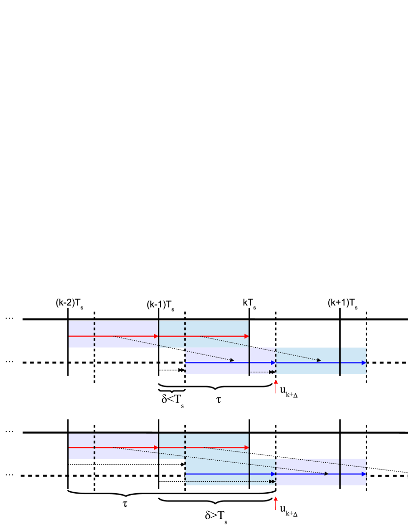
The controller is applied in real-time by computing, at iteration $k$ for either case $\delta\geq T_{s}$ or $\delta\leq T_{s}$,

$$\widehat{{\boldsymbol{\psi}}}_{k+1|k}({\boldsymbol{\alpha}}) ={\mathbf{A}}\widehat{{\boldsymbol{\psi}}}_{k|k-1}({\boldsymbol{\alpha}})+{\mathbf{A}}\mathcal{H}_{\infty}\left({\mathbf{s}}_{k}({\boldsymbol{\alpha}})-\mathbf{G}\widehat{{\boldsymbol{\psi}}}_{k|k-1}({\boldsymbol{\alpha}})\right)$$ (27a)

$${\mathbf{u}}_{k+\delta/T_{s}}({\boldsymbol{\beta}}_{i}) =\mathbf{F}\boldsymbol{\Sigma}_{{\boldsymbol{\psi}}_{{\boldsymbol{\beta}}_{i}},{\boldsymbol{\psi}}_{\boldsymbol{\alpha}}}\boldsymbol{\Sigma}_{{\boldsymbol{\psi}}_{\boldsymbol{\alpha}},{\boldsymbol{\psi}}_{\boldsymbol{\alpha}}}^{-1}{\mathbf{A}}_{\delta}\widehat{{\boldsymbol{\psi}}}_{k+1|k}({\boldsymbol{\alpha}})$$

$$=\mathbf{T}_{\delta}\widehat{{\boldsymbol{\psi}}}_{k+1|k}({\boldsymbol{\alpha}})$$ (27b)

where ${\mathbf{A}}_{\delta}$ estimates the lead wave-front $\delta$ seconds ahead in time to overcome any pure lag delay (3ms for the case of Raven) and multiplication by the anisoplanatic filter $\boldsymbol{\Sigma}_{{\boldsymbol{\psi}}_{\boldsymbol{\beta}},{\boldsymbol{\psi}}_{\boldsymbol{\alpha}}}\boldsymbol{\Sigma}_{{\boldsymbol{\psi}}_{\boldsymbol{\alpha}},{\boldsymbol{\psi}}_{\boldsymbol{\alpha}}}^{-1}=\left\langle{{\boldsymbol{\psi}}({\boldsymbol{\beta}}){\boldsymbol{\psi}}({\boldsymbol{\alpha}})^{\mathsf{T}}}\right\rangle\left\langle{{\boldsymbol{\psi}}({\boldsymbol{\alpha}}){\boldsymbol{\psi}}({\boldsymbol{\alpha}})^{\mathsf{T}}}\right\rangle^{-1}$ provides the pupil-plane wave-front estimate in the science direction of interest. This two-step scheme is equivalent to a single-step prediction on account of the conditional expectation properties, namely

$$E\{\Phi|S=s\}=E\{\Phi|E\{Y|S=s\}\}$$ (28)

The DM projection is made in parallel for all the $N_{\beta}$ science directions by multiplying by the generalized inverse of the DM influence matrix in Eq. (II.3).

III Static and predictive Spatio-Angular wave-front estimation

The state-space framework offers a suitable means to derive static reconstructors against which we will compare the LQG formulation. The presentation that follows is a brief review of the standard minimisation criteria in AO that can be found elsewhere piatrou07 ; whiteley98a ; ellerbroek02 ; correia14 . Here we derive it seamlessly from choosing a specific combination of matrices in the LQG controller to set the context for the simulation results that ensue.

III.1 Static case

It is a well established result that the static minimum mean square error MMSE solution correia14

$$\widehat{{\boldsymbol{\psi}}}_{\boldsymbol{\beta}} \triangleq\boldsymbol{\Sigma}_{{\boldsymbol{\psi}}_{\boldsymbol{\beta}},{\mathbf{s}}_{\boldsymbol{\alpha}}}\boldsymbol{\Sigma}^{-1}_{{\mathbf{s}}_{\boldsymbol{\alpha}},{\mathbf{s}}_{\boldsymbol{\alpha}}}{{\mathbf{s}}}_{\boldsymbol{\alpha}}$$ (29)

$$=\left\langle{{\boldsymbol{\psi}}_{\boldsymbol{\beta}}{\boldsymbol{\psi}}_{\boldsymbol{\alpha}}^{\mathsf{T}}}\right\rangle\mathbf{G}^{\mathsf{T}}\left(\mathbf{G}\left\langle{{\boldsymbol{\psi}}_{\boldsymbol{\alpha}}{\boldsymbol{\psi}}_{\boldsymbol{\alpha}}^{\mathsf{T}}}\right\rangle\mathbf{G}^{\mathsf{T}}+\left\langle{{\boldsymbol{\eta}}{\boldsymbol{\eta}}^{\mathsf{T}}}\right\rangle\right)^{-1}{{\mathbf{s}}}_{\boldsymbol{\alpha}}$$ (30)

can be derived from the LQG solution by taking $\mathcal{A}=\mathsf{0}$ and therefore the conditional expectation $\widehat{{\boldsymbol{\psi}}}_{k|k-1}=\mathsf{0}$ in Eq. (27). In such case the solution of the Riccati equation is $\Sigma_{\infty}=\Sigma_{\boldsymbol{\varphi}}$ and the Kalman gain boils down to

$$\mathcal{H^{\prime}}_{\infty}=\left\langle{{\boldsymbol{\psi}}_{\boldsymbol{\beta}}{\boldsymbol{\psi}}_{\boldsymbol{\alpha}}^{\mathsf{T}}}\right\rangle\mathbf{G}^{\mathsf{T}}\left(\mathbf{G}\left\langle{{\boldsymbol{\psi}}_{\boldsymbol{\alpha}}{\boldsymbol{\psi}}_{\boldsymbol{\alpha}}^{\mathsf{T}}}\right\rangle\mathbf{G}^{\mathsf{T}}+\left\langle{{\boldsymbol{\eta}}{\boldsymbol{\eta}}^{\mathsf{T}}}\right\rangle\right)^{-1}$$ (31)

which provides the same resulting estimate phase vector as in Eq. (29).

III.2 Predictive case

To reduce the lag error, spatio-temporal prediction may be built-in the reconstructor. In such case one computes instead vogel04a

$$\widehat{{\boldsymbol{\psi}}}_{k+\Delta}({\boldsymbol{\beta}}) \triangleq\left\langle{{\boldsymbol{\psi}}_{k+\Delta}({\boldsymbol{\beta}}){\mathbf{s}}_{k}^{\mathsf{T}}({\boldsymbol{\alpha}})}\right\rangle\boldsymbol{\Sigma}^{-1}_{{\mathbf{s}}_{\boldsymbol{\alpha}},{\mathbf{s}}_{\boldsymbol{\alpha}}}$$ (32)

where $\left\langle{{\boldsymbol{\psi}}_{k+\Delta}({\boldsymbol{\beta}}){\mathbf{s}}_{k}^{\mathsf{T}}({\boldsymbol{\alpha}})}\right\rangle=\left\langle{{\boldsymbol{\psi}}(\boldsymbol{\rho}-\mathbf{v}\tau,{\boldsymbol{\beta}}){\mathbf{s}}^{\mathsf{T}}({\boldsymbol{\alpha}})}\right\rangle$ is the covariance matrix of pupil-plane phase between the science and guide-star directions at two time instants separated by a lag $\tau$.

Equation (32) can be split into a spatial estimate followed by a temporal prediction step, being written in the two-step form

$$\widehat{{\boldsymbol{\psi}}}_{k+\Delta}({\boldsymbol{\beta}}) ={\mathbf{A}}_{\Delta}\widehat{{\boldsymbol{\psi}}}_{k}({\boldsymbol{\beta}})$$ (33)

$$={\mathbf{A}}_{\Delta}\boldsymbol{\Sigma}_{{\boldsymbol{\psi}}_{\boldsymbol{\beta}},{\mathbf{s}}_{\boldsymbol{\alpha}}}\boldsymbol{\Sigma}^{-1}_{{\mathbf{s}}_{\boldsymbol{\alpha}},{\mathbf{s}}_{\boldsymbol{\alpha}}}{{\mathbf{s}}}_{\boldsymbol{\alpha}}$$ (34)

Both this two-step approach or the all-at-once are equivalent as pointed out before due to conditional expectation properties. It remains true however many steps are made as long as the starting point is a pupil-plane phase estimate.

IV Computational aspects

IV.1 Off-line computation of Spatio-Angular covariance matrices

The point-wise covariance matrix computation involves only spatial distances from which the spatio-angular covariances matrices are obtained analytically sampling the covariance function for von-Kármán turbulence

$$C_{\psi}(\rho)=\left(\frac{L_{0}}{r_{0}}\right)^{5/3}\times\frac{\Gamma(11/6)}{2^{5/6}\pi^{8/3}}\left[\frac{24}{5}\Gamma\left(\frac{6}{5}\right)\right]\left(\frac{2\pi\rho}{L_{0}}\right)^{5/6}K_{5/6}\left(\frac{2\pi\rho}{L_{0}}\right)$$ (35)

with $L_{0}$ the outer scale of turbulence, $r_{0}$ Fried’s parameter, $\Gamma$ the ’gamma’ function and finally $K_{5/6}$ a modified Bessel function of the third order. Parameter $\rho=|\boldsymbol{\rho}|$ is the distance between two phase points in the bi-dimensional plane $\rho=\sqrt{\Delta x^{2}+\Delta y^{2}}$.

For the multiple-layer case, the pupil-plane covariance functions are found from the weighted sum over the layers where the weighting is given by the relative strength of layer $l$ (also known as the fractional $r_{0}$).

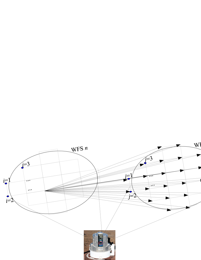
The spatio-angular covariance matrices are found by sampling and stacking the analytical covariance function in Eq. (35) layer-by-layer (since layers are considered independent) between points tracing to the WFS sub-apertures’ corners and mid-points whose coordinates in any layer are,$[(\rho_{x_{i,n}}+\theta_{x_{n}}h_{\mathit{l}}),(\rho_{y_{i,n}}+\theta_{y_{n}}h_{\mathit{l}})$ and the separation vector between sub-aperture raster index $i$ on WFS $n$ and sub-aperture $j$ on WFS $m$ at layer $\mathit{l}$ is,

$$\boldsymbol{\rho}_{i,j,l}=(\boldsymbol{\rho}_{i,n}-\boldsymbol{\rho}_{j,m})+h_{\mathit{l}}({\boldsymbol{\theta}}_{n}-{\boldsymbol{\theta}}_{m}),$$ (36)

where the first term of the right hand side of the equation is the separation between the sub-apertures in the pupil and the second term is the global WFS separation vector back-projected in the atmosphere. Figure 3 provides a schematic view of that procedure.

Figure 3: Spatio-angular computation scheme. Each column in the covariance matrix is obtained by sampling the phase covariance function with distances corresponding to the length of the arrows as shown. To comply with the 3x3 stencil in the gradient operator, the corners and the mid-points are sampled.

IV.2 Real-time computational burden: scaling laws

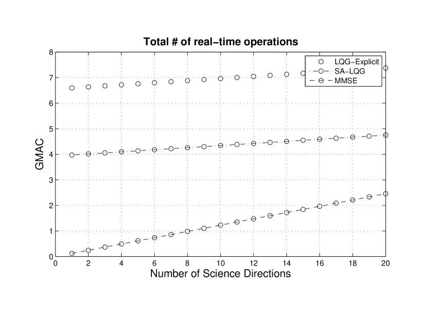
Regarding computational complexity, the SA-LQG formulation offers a reduced number of real-time operations compared to the E-LQG formulation. Furthermore it provides less than one order of magnitude increase compared to MMSE (static or predictive) reconstructors for a ELT-sized case with a multiplexing factor of 20.

Take ${{N_{\beta}}}$ to be the number of DM or likewise science directions; ${{N_{\text{act}}}}$ the number of valid actuators per DM; ${{N_{\alpha}}}$ the number of GS directions; ${{N_{\text{s}}}}\approx 2{{N_{\text{act}}}}$ the number of slope measurements per WFS; ${{N}_{\varphi}}=4{{N_{\text{act}}}}$ is an under-estimate of the number of phase points estimated per reconstructed layer and ${{N_{\text{l}}}}$ the total number of layers. Table 1 provides the approximate number of real-time multiply-and-accumulate (MAC) operations.

Table 1: Approximate real-time computational complexity.

Op. / Algo.	SA-LQG	E-LQG	MMSE
$\mathcal{C}\widehat{{\mathbf{x}}}_{k|k-1}$	$9{{N_{\text{s}}}}{{N_{\alpha}}}$	$9{{N_{\text{s}}}}{{N_{\alpha}}}+4{{N}_{\varphi}}{{N_{\text{l}}}}$
${\mathbf{A}}\mathcal{H}_{\infty}$	${{N_{\alpha}}}{{N}_{\varphi}}{{N_{\text{s}}}}{{N_{\alpha}}}$	${{N_{\text{l}}}}{{N}_{\varphi}}{{N_{\text{s}}}}{{N_{\alpha}}}$	${{N_{\beta}}}{{N_{\text{act}}}}{{N_{\alpha}}}{{N_{\text{s}}}}$
${\mathbf{A}}{\mathbf{x}}_{k|k}$	$4{{N}_{\varphi}}{{N_{\alpha}}}$	$4{{N}_{\varphi}}{{N_{\text{l}}}}$
$\mathbf{F}{\mathbf{x}}_{k+1|k}$	${{N_{\beta}}}{{N_{\text{act}}}}{{N}_{\varphi}}$	${{N_{\beta}}}{{N_{\text{act}}}}{{N}_{\varphi}}+4{{N_{\text{l}}}}{{N}_{\varphi}}$

If we take the case of Raven with ${{N_{\beta}}}=2$, ${{N_{\text{act}}}}=97$, ${{N_{\alpha}}}=3$, ${{N_{\text{s}}}}=144$ we get an increased computational complexity of about a factor 15 for the SA-LQG and 30 for the E-LQG controller with 9 layers.

As an example Fig. 4 shows the scaling complexity for ELT-sized systems (e.g. E-ELT MOSAIC 14, TMT’s IRMOS andersen06 ) as a function of the number of science targets for ${{N_{\text{act}}}}=3200$ (from a 64x64 DM), ${{N_{\text{s}}}}=2{{N_{\text{act}}}}$, ${{N}_{\varphi}}=4{{N_{\text{act}}}},$${{N_{\text{l}}}}=10$ and ${{N_{\alpha}}}=6$. For a maximum multiplex capacity of 20 science targets both the SA-LQG and the E-LQG are only a factor 2 and 3 more demanding than the MMSE, i.e. roughly the same complexity. We have only considered the MMSE implemented as a full VMM since there is growing evidence that this option maps well into GPUs and should therefore be preferred to iterative implementations veran14 . For the time being we exclude from this analysis other considerations such as memory bandwidth and pipelinability.

Figure 4: Number of Giga multiply-and-accumulate (GMAC) real-time operations required by the LQG when compared to the static/predictive MMSE and the Explicit LQG. 3200 actuators, 6 WFS with 2x3200 slopes per WFS, phase estimated over 2x number of actuators per DM, 10 layers

V Sample numerical models and simulations

An end-to-end Monte Carlo wave-optics simulation of the Raven tomographic system in a zonal basis has been set up using the object-oriented OOMAO simulator conanr14 to examine the performance of the SA-LQG algorithm in relation to simpler static and predictive reconstructors.

V.1 Model Parameters and Validation

The figure-of-merit we use to establish the quality of the wavefront correction is the ensquared energy (EE); this is computed as the ratio of the amount of light falling on a science camera within a given angle projected on-sky to the total amount of light reaching the detector. Strehl ratios are also computed for completeness.

Table 2 contains the main simulation parameters, selected to reflect the physical properties available in the Calibration Unit of our Raven system test-bench andersen12a . These include a three layer atmosphere located at ground, 5.5 and 11 km altitudes, an turbulence coherence length $r_{0}$ of 19 cm and an atmospheric outer scale $L_{0}$ of 40 m.

Table 2: Raven Baseline Configuration Parameters.

Telescope
D	8 m
Atmosphere
$r_{0}$	19 cm
$L_{0}$	40 m
zenith angle	0 deg
Fractional $r_{0}$	[0.596; 0.224; 0.180]
Altitudes	[0, 5.5, 11] km
wind speeds	[5.68; 6; 17] m/s
wind direction	[90; 180;180] deg
Wavefront Sensor
$N_{NGS}$	3
Order	10$\times$10
$\theta_{pix}$	0.4 arcsec
RON	0.2 e-
NGS radii	45 arcsec
$N_{pix}$	12
$f_{sample}$	30-200 Hz
$\lambda_{WFS}$	0.64 $\mu$m
Centroiding algorithm	thresholded Centre-of-Gravity
DM
$N_{DM}$	2
Order	11$\times$11
stroke	infinite
influence	cubic
AO loop
pure delay	$\tau_{\mathsf{lag}}=$ 3ms
Evaluation Wavelength
$\lambda_{evl}$	1.65 $\mu$m

Model behavior was verified by collecting a simulated long exposure science image using no AO correction mode. The theoretical estimate of the Full Width at Half Max (FWHM) of the long exposure PSF for the baseline atmosphere in J band (1.2 $\mu m$) can be computed for a finite outer scale using the expression developed in tokovinin02 for the ratio, $L_{0}/r_{0}>20$. With $r_{0}=0.156cm$ at $0.5\mu m$ and $L_{0}=30m$ (chosen from median conditions on Mauna Kea), this computation yields an expected FWHM of 0.3891 arc seconds in J-band. The FWHM of a simulated long exposure science image was computed to be 0.3865 arc seconds, confirming good agreement between theory and simulation. Note that this test was carried during initial validation of the simulation tools before parameters such as $r_{0}$ were finalized.

V.2 Results

Previous work correia14 examined the trade-off between lower WFS frame-rates which reduces spatial errors due to noise propagation since measurement’s SNR is higher but increases temporal lag error. Correction quality was shown to increase with WFS integration time to a point and then begin to decrease as the lag error exceeded the SNR gain.

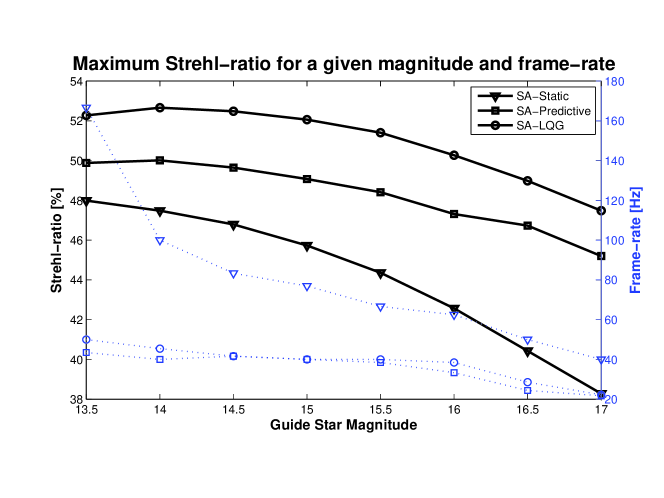
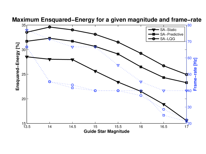
Table 3 summarizes the peak performances over the frame-rates for varying GS magnitudes.

Table 3: Raven End-to-End simulation results. The optimal performance ( % ensquared energy) for each GS magnitude is shown for the zonal static SA, and compared to stand-alone SA Prediction and the full SA LQG algorithm.

GS mags	static SA				SA Prediction				SA LQG
	EE	lag	Strehl	lag	EE	lag	Strehl	lag	EE	lag	Strehl	lag
13.5	47.99	6	28.55	13	49.88	23	31.70	15	52.27	20	33.54	15
14	47.48	10	28.05	14	50.01	25	32.32	22	52.66	22	34.60	22
14.5	46.79	12	27.98	15	49.65	24	31.72	24	52.48	24	34.02	23
15	45.73	13	25.64	15	49.07	25	30.66	25	52.06	25	33.12	25
15.5	44.36	15	23.41	18	48.41	26	29.11	25	51.40	25	31.53	25
16	42.57	16	21.52	22	47.31	30	26.50	25	50.27	26	29.25	27
16.5	40.43	20	18.90	25	46.73	41	24.33	40	48.98	35	26.72	35
17	38.28	25	15.57	25	45.20	46	23.29	47	47.48	45	24.95	45

These tests show that, as in the modal case, better peak performance can be achieved using temporal prediction and this peak occurs at lower frame-rates than the static algorithm for each magnitude. Providing reduced noise-propagation the SA-LQG algorithm shows that the best performance occurs at approximately the same WFS frame-rate as in the predictive case, but that overall performance is significantly improved, indicating a reduction in spatial error. The data is also plotted in Fig. 5; here it can be seen that by using temporal prediction equivalent performance can be achieved with higher magnitude GSs when using a lower frame-rate. The LQG can deliver performance equivalent to that of the predictive algorithm using GSs which are one magnitude dimmer and equivalent to the static algorithm using GSs which are greater than two magnitudes dimmer.

Figure 5: Static reconstructor vs Stand-alone Prediction and LQG: Strehl ratios (top) and ensquared energy (bottom) as a function of NGS magnitude. Left axis shows best achieved performance with a static reconstructor compared to the predictive and LQG reconstructors; right axis shows the OL-WFS sample rate at which that performance is obtained.

V.3 SA-LQG v. E-LQG

In appendix A it is shown that the SA-LQG can be deduced from the E-LQG (under certain conditions) in a stationary regime.

The geometrical nature of the problem, however, is such that we can retrieve the pupil-plane wave-front from its layered counterpart through ray-tracing but not the opposite. This is patent in the noninvertibility of $\mathbf{H}$ which imposes a spatial truncation on the wave-fronts over the footprints in the GS direction otherwise represented on larger meta-pupils.

Simulations have shown that

$$\left\langle{\|\psi_{k}({\boldsymbol{\alpha}})-\widehat{\psi}_{k|k}({\boldsymbol{\alpha}})\|^{2}}\right\rangle\geq\left\langle{\|\psi_{k}({\boldsymbol{\alpha}})-\mathbf{H}_{\boldsymbol{\alpha}}\widehat{{\boldsymbol{\varphi}}}_{k|k}\|^{2}}\right\rangle$$ (37)

i.e., the averaged residual phase variance in the GS directions obtained with the SA-LQG is higher than the one obtained with the E-LQG. This difference then translates to the science when using the anisoplanatic filter as follows

$$\left\langle{\|\psi_{k}({\boldsymbol{\beta}})-\boldsymbol{\Sigma}_{\boldsymbol{\rho}_{\boldsymbol{\beta}},\boldsymbol{\rho}_{\boldsymbol{\alpha}}}\boldsymbol{\Sigma}_{\boldsymbol{\rho}_{\boldsymbol{\alpha}},\boldsymbol{\rho}_{\boldsymbol{\alpha}}}^{-1}\widehat{\psi}_{k|k}({\boldsymbol{\alpha}})\|^{2}}\right\rangle\geq\left\langle{\|\psi_{k}({\boldsymbol{\beta}})-\mathbf{H}_{\boldsymbol{\beta}}\widehat{{\boldsymbol{\varphi}}}_{k|k}\|^{2}}\right\rangle$$ (38)

The anisoplanatic filter per se adds no further error to the estimation since

$$\left\langle{\|\psi_{k}({\boldsymbol{\beta}})-\boldsymbol{\Sigma}_{\boldsymbol{\rho}_{\boldsymbol{\beta}},\boldsymbol{\rho}_{\boldsymbol{\alpha}}}\boldsymbol{\Sigma}_{\boldsymbol{\rho}_{\boldsymbol{\alpha}},\boldsymbol{\rho}_{\boldsymbol{\alpha}}}^{-1}\mathbf{H}_{\boldsymbol{\alpha}}\widehat{{\boldsymbol{\varphi}}}_{k|k}\|^{2}}\right\rangle=\left\langle{\|\psi_{k}({\boldsymbol{\beta}})-\mathbf{H}_{\boldsymbol{\beta}}\widehat{{\boldsymbol{\varphi}}}_{k|k}\|^{2}}\right\rangle$$ (39)

A modal decomposition of the errors using Zernike polynomials showed that the low-order modes such as tilts, focus and astigmatism are more affected. This is also in agreement with the little impact in EE observed which would suffer more from poorer correction of high order modes.

For the Raven case, the differences observed in the science direction are of the percent level.

VI Raven Laboratory Test Results

Raven’s physical design and system capabilities are summarized in jackson12 ; andersen12a ; andersen12 ; it is equipped with a calibration unit (CU) which also serves as a telescope simulator and turbulence generator. A broad spectrum source illuminates an array of pinholes, any three of which can be picked off to create an NGS asterism, and a series of filters which allow incremental changes in the magnitudes of all asterism stars at once. A cross section of measurements across NGS WFS frame rates were taken for three different filters to show the improvement in performance using prediction and SA-LQG control over the static reconstructor. The laboratory results also validate our simulation results which indicate that, using the SA-LQG reconstructor, the system can produce performance equivalent to that obtained using the static reconstructor when GSs are 2 magnitudes fainter. A plot of the results of these measurements is shown in Fig. 6. The diameter of the asterism used is approximately 2 arminutes. The CU lamp does not illuminate all pinholes with uniform intensity, therefore the data points labeled Mag 13 were generated using GSs with magnitudes [12.6,13.25, 13.25]; those labeled Mag 15 are actually [14.3, 15, 15], and those labeled Mag 17 are [16.5, 17.2, 17.2].

Figure 6: Measured ensquared energy in a 140 milliarcsecond slit of science images taken while running the NGS WFSs at varying frame rates and executing static, predictive and LQG algorithms at three different magnitude settings. The static reconstructor results are not shown for the faintest stars as the performance is not better than no AO correction.

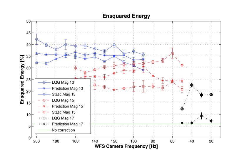
The performance achieved in lab tests is lower than that predicted by simulations in all reconstructor cases. However the trend of increasing peak performance with each increase in reconstructor complexity is reflected in both the simulation data and the measured data. The overall decrease in performance can be attributed to multiple sources; these include imperfect calibration, which has a significant impact on OL systems, underestimation of noise sources in the simulation compared to reality, effects of the rotated WFSs, DM fitting, OL go-to errors, and non-common path aberrations (NCPA) between the OL and science paths, as well as between the CL-WFSs and the science camera. A higher amount of total system lag than anticipated may also be reducing the performance of all three types of reconstructors. Albeit, the main simulation findings in improved performance could be reproduced with the test-bench. We are currently investigating ways of enhancing the calibration and fine knowledge of system parameters in order to optimize overall system performance and gain understanding over unmodelled system features.

Figure 7: Comparison of Science camera images for SA-LQG, Predictive and Static tomographic reconstruction algorithms. Peak frequency PSF shown for each reconstructor using magnitude 15 NGSs (see Fig. 6) .

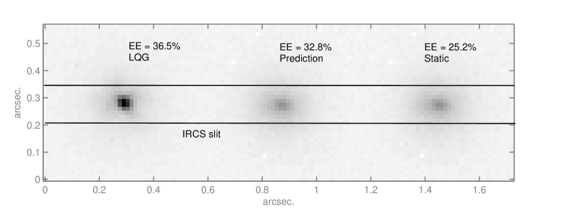
The science images in Fig. 7 represent the best performance achieved for each reconstruction method for a fixed magnitude; they clearly show that the EE is increased and the spot image becomes smaller for both predictive and LQG algorithms over the static reconstructor.

VII Summary

We have outlined the dynamical Strehl-optimal LQG controller providing minimum residual phase variance tailored to MOAO systems. The latter does not require explicit knowledge of the tridimensional wave-front profile allowing for a simplified forward model. Our implementation uses anisoplanatic filters to estimate pupil-plane wave-front profiles from any other directions based on knowledge of the turbulent $C_{n}^{2}$ profile. One such approach can also be useful for laser tomography AO.

We have included temporal prediction by assuming frozen-flow, in which case time evolution can be converted to spatial translations. We have proposed a minimal space-state representation with a single temporal instance providing reduced computational complexity.

By allowing the controller to run slower while performing temporal prediction, we can increase the SNR in the wave-front measurements by collecting more light in each sensor’s sub-apertures. We have shown that we could gain two magnitudes for a same performance obtained with a MMSE static reconstructor, leading to a sky-coverage improvement of roughly a factor 5.

Appendix A Relationships between SA and Explicit LQG

We set forth to show that the SA-LQG formulation provided in this paper shares important features with the more standard “explicit” E-LQG formulation which involves the estimation of phase in the layers.

Let the E-LQG state update equation

$$\widehat{{\boldsymbol{\varphi}}}_{k+1|k} ={\mathbf{A}_{\text{\tiny{E}}}}\widehat{{\boldsymbol{\varphi}}}_{k|k-1}+{\mathcal{L}_{\infty}^{\text{\tiny{E}}}}(s_{k}-\mathbf{G}\mathbf{H}\widehat{{\boldsymbol{\varphi}}}_{k|k-1})$$ (40)

where upper/subscript ’E’ indicates matrices for the E-LQG case.

For the near-Markovian order 1 time-progression model assumed earlier, the driving noise statistics are such that $\boldsymbol{\Sigma}_{n}^{\mathsf{E}}=\boldsymbol{\Sigma}_{\boldsymbol{\varphi}}-{\mathbf{A}_{\text{\tiny{E}}}}\boldsymbol{\Sigma}_{\boldsymbol{\varphi}}{\mathbf{A}_{\text{\tiny{E}}}^{\mathsf{T}}}$. Multiplying out by the ray-tracing operator to the left and its transpose to the right equates to $\boldsymbol{\Sigma}_{n}=\boldsymbol{\Sigma}_{\boldsymbol{\psi}}-{\mathbf{A}}\boldsymbol{\Sigma}_{\boldsymbol{\psi}}{\mathbf{A}}^{\mathsf{T}}$ by plausibly taking

$${\mathbf{A}} =\mathbf{H}{\mathbf{A}_{\text{\tiny{E}}}}\mathbf{H}^{{\dagger}}$$ (41)

and assuming $\mathbf{H}^{{\dagger}}$ to be computable and furthermore that $\mathbf{H}\mathbf{H}^{{\dagger}}=\mathbf{I}$. This assumption however may not hold since $\mathbf{H}$ is non-squared and its structure gives rise to a rank deficient matrix. We thus expect (and have evidence for) some differences using the SA-LQG with respect to the E-LQG formulation.

We now add the following

$$\mathbf{H}{\mathbf{A}_{\text{\tiny{E}}}} =\mathbf{H}(\mathbf{H}^{{\dagger}}{\mathbf{A}}\mathbf{H})$$ (42)

$$={\mathbf{A}}\mathbf{H}$$ (43)

and

$$\mathbf{H}\mathcal{L}_{\infty} =\mathbf{H}{\mathbf{A}_{\text{\tiny{E}}}}{\mathcal{M}_{\infty}^{\text{\tiny{E}}}}$$ (44)

$$={\mathbf{A}}\mathbf{H}{\mathcal{M}_{\infty}^{\text{\tiny{E}}}}$$ (45)

$$={\mathbf{A}}\mathcal{M}_{\infty}$$ (46)

Multiplying the state update equation on both sides by $\mathbf{H}$ to the left equates to

$$\mathbf{H}\widehat{{\boldsymbol{\varphi}}}_{k+1|k} =\mathbf{H}{\mathbf{A}_{\text{\tiny{E}}}}\widehat{{\boldsymbol{\varphi}}}_{k|k-1}+\mathbf{H}{\mathcal{L}_{\infty}^{\text{\tiny{E}}}}({\mathbf{s}}_{k}-\mathbf{G}\mathbf{H}\widehat{{\boldsymbol{\varphi}}}_{k|k-1})$$ (47)

$$=\mathbf{H}({\mathbf{A}_{\text{\tiny{E}}}}-{\mathcal{L}_{\infty}^{\text{\tiny{E}}}}\mathbf{G}\mathbf{H})\widehat{{\boldsymbol{\varphi}}}_{k|k-1}+\mathbf{H}{\mathcal{L}_{\infty}^{\text{\tiny{E}}}}{\mathbf{s}}_{k}$$ (48)

With the above identities one gets $\mathbf{H}{\mathcal{L}_{\infty}^{\text{\tiny{E}}}}\mathbf{G}\mathbf{H}\widehat{{\boldsymbol{\varphi}}}_{k|k-1}={\mathbf{A}}{\mathcal{M}_{\infty}}\mathbf{G}\widehat{{\boldsymbol{\psi}}}_{k|k-1}$, yielding

$$\widehat{{\boldsymbol{\psi}}}_{k+1|k} ={\mathbf{A}}(\mathbf{I}-{\mathcal{M}_{\infty}}\mathbf{G})\widehat{{\boldsymbol{\psi}}}_{k|k-1}+{\mathcal{M}_{\infty}}{\mathbf{s}}_{k}$$ (49)

which is the SA formulation.

We are left with the derivation of equivalence of Kalman gains and respective Riccati solutions, both computed off-line. The Riccati equation writes

$${\boldsymbol{\Sigma}_{\infty}^{\text{\tiny{E}}}} ={\mathbf{A}_{\text{\tiny{E}}}}{\boldsymbol{\Sigma}_{\infty}^{\text{\tiny{E}}}}{\mathbf{A}_{\text{\tiny{E}}}^{\mathsf{T}}}+{\boldsymbol{\Sigma}_{n}^{\text{\tiny{E}}}}-{\mathbf{A}_{\text{\tiny{E}}}}{\boldsymbol{\Sigma}_{\infty}^{\text{\tiny{E}}}}\mathbf{H}^{\mathsf{T}}\mathbf{G}^{\mathsf{T}}$$

$$\left(\mathbf{G}\boldsymbol{\Sigma}_{\infty}\mathbf{G}^{\mathsf{T}}+\boldsymbol{\Sigma}_{\eta}\right)^{-1}\mathbf{G}\mathbf{H}{\boldsymbol{\Sigma}_{\infty}^{\text{\tiny{E}}}}{\mathbf{A}_{\text{\tiny{E}}}}^{\mathsf{T}}$$ (50)

Multiplying by $\mathbf{H}$ on the left and $\mathbf{H}^{\mathsf{T}}$ on the right one gets immediately

$${\boldsymbol{\Sigma}_{\infty}} ={\mathbf{A}}{\boldsymbol{\Sigma}_{\infty}}{\mathbf{A}}^{\mathsf{T}}+{\boldsymbol{\Sigma}_{n}}$$ (51)

$$-{\mathbf{A}}{\boldsymbol{\Sigma}_{\infty}}\mathbf{G}^{\mathsf{T}}\left(\mathbf{G}{\boldsymbol{\Sigma}_{\infty}}\mathbf{G}^{\mathsf{T}}+\boldsymbol{\Sigma}_{\eta}\right)^{-1}\mathbf{G}{\boldsymbol{\Sigma}_{\infty}}{\mathbf{A}}^{\mathsf{T}}$$ (52)

where we take ${\boldsymbol{\Sigma}_{\infty}}=\mathbf{H}{\boldsymbol{\Sigma}_{\infty}^{\text{\tiny{E}}}}\mathbf{H}^{\mathsf{T}}$ with the state noise covariance matrix in the SA case obtained from the E-LQG using the definitions above. In practice this assumption does not hold in part due to the finite number of iterations used to compute the asymptotic Riccati estimation error covariance matrix $\boldsymbol{\Sigma}_{\infty}$ and its E-LQG counterpart, in part since the geometry of the problem imposes a spatial truncation on baselines over which covariances are computed unfavourable to the SA-LQG.

The Kalman gain can then be obtained as

$$\mathbf{H}{\mathcal{M}_{\infty}^{\text{\tiny{E}}}} =\mathbf{H}{\boldsymbol{\Sigma}_{\infty}^{\text{\tiny{E}}}}\mathbf{H}^{\mathsf{T}}\mathbf{G}^{\mathsf{T}}\left(\mathbf{G}\mathbf{H}{\boldsymbol{\Sigma}_{\infty}^{\text{\tiny{E}}}}\mathbf{H}^{\mathsf{T}}\mathbf{G}^{\mathsf{T}}+\boldsymbol{\Sigma}_{\eta}\right)^{-1}$$ (53)

$${\mathcal{M}_{\infty}} ={\boldsymbol{\Sigma}_{\infty}}\mathbf{G}^{\mathsf{T}}\left(\mathbf{G}{\boldsymbol{\Sigma}_{\infty}}\mathbf{G}^{\mathsf{T}}+\boldsymbol{\Sigma}_{\eta}\right)^{-1}$$ (54)

which is the straight SA formulation.

Further to the results shown in Sect. V.3, by using the Kalman gain for the SA-LQG from Eq. (53) does not change the performances reported.

References

- (1) C. Correia, K. Jackson, J.-P. Véran, D. Andersen, O. Lardière, and C. Bradley, “Static and predictive tomographic reconstruction for wide-field multi-object adaptive optics systems,” J. Opt. Soc. Am. A 31, 101–113 (2014).
- (2) F. Vidal, E. Gendron, and G. Rousset, “Tomography approach for multi-object adaptive optics,” J. Opt. Soc. Am. A 27, A253–A264 (2010).
- (3) D. R. Andersen, K. J. Jackson, C. Blain, C. Bradley, C. Correia, M. Ito, O. Lardière, and J.-P. Véran, “Performance modeling for the raven multi-object adaptive optics demonstrator,” Publications of the Astronomical Society of the Pacific 124, pp. 469–484 (2012).
- (4) G. Sivo, C. Kulcsár, J.-M. Conan, H.-F. Raynaud, Éric Gendron, A. Basden, F. Vidal, T. Morris, S. Meimon, C. Petit, D. Gratadour, O. Martin, Z. Hubert, A. Sevin, D. Perret, F. Chemla, G. Rousset, N. Dipper, G. Talbot, E. Younger, R. Myers, D. Henry, S. Todd, D. Atkinson, C. Dickson, and A. Longmore, “First on-sky scao validation of full LQG control with vibration mitigation on the canary pathfinder,” Opt. Express 22, 23565–23591 (2014).
- (5) D. R. Andersen, S. S. Eikenberry, M. Fletcher, W. Gardhouse, B. Leckie, J.-P. Véran, D. Gavel, R. Clare, R. Guzman, L. Jolissaint, R. Julian, and W. Rambold, “The MOAO system of the IRMOS near-infrared multi-object spectrograph for TMT,” in “Proc. of the SPIE,” , vol. 6269 (2006), vol. 6269, pp. 62694K–62694K–12.
- (6) F. Hammer, B. Barbuy, J. G. Cuby, L. Kaper, S. Morris, C. J. Evans, P. Jagourel, G. Dalton, P. Rees, M. Puech, M. Rodrigues, D. Pearson, and K. Disseau, “MOSAIC at the E-ELT: A multi-object spectrograph for astrophysics, IGM and cosmology,” in “Proc. SPIE,” , vol. 9147 (2014), vol. 9147, p. 27.
- (7) K. Jackson, C. Correia, O. Lardière, D. Andersen, and C. Bradley, “Linear prediction of atmospheric wave-fronts for tomographic adaptive optics systems: modelling and robustness assessment,” Opt. Lett. 40, 143–146 (2015).
- (8) P. Piatrou and L. Gilles, “Robustness study of the pseudo open-loop controller for multiconjugate adaptive optics,” Appl. Opt. 44, 1003–1010 (2005).
- (9) C. Correia, H.-F. Raynaud, C. Kulcsár, and J.-M. Conan, “On the optimal reconstruction and control of adaptive optical systems with mirroir dynamics,” J. Opt. Soc. Am. A 27, 333–349 (2010).
- (10) L. Gilles, P. Massioni, C. Kulcsár, H.-F. Raynaud, and B. Ellerbroek, “Distributed Kalman filtering compared to Fourier domain preconditioned conjugate gradient for laser guide star tomography on extremely large telescopes,” J. Opt. Soc. Am. A 30, 898 (2013).
- (11) C. Correia, J.-M. Conan, C. Kulcsár, H.-F. Raynaud, and C. Petit, “Adapting optimal LQG methods to ELT-sized AO systems,” in “1st AO4ELT Conference - Adaptative Optics for Extremely Large Telescopes proceedings,” , T. F. Y. Clénet, J.-M. Conan and G. Rousset, eds. (EDP Sciences, 2009), 07003.
- (12) L. Gilles, C. R. Vogel, and B. L. Ellerbroek, “Multigrid preconditioned conjugate-gradient method for large-scale wave-front reconstruction,” J. Opt. Soc. Am. A 19, 1817–1822 (2002).
- (13) B. L. Ellerbroek, “A wave optics propagation code for multi-conjugate adaptive optics,” in “European Southern Observatory Conference and Workshop Proceedings,” , vol. 58, E. Vernet, R. Ragazzoni, S. Esposito, and N. Hubin, eds. (2002), vol. 58, p. 239.
- (14) B. L. Ellerbroek, “Efficient computation of minimum-variance wave-front reconstructors with sparse matrix techniques,” J. Opt. Soc. Am. A 19, 1803–1816 (2002).
- (15) C. Kulcsár, H.-F. Raynaud, C. Petit, J.-M. Conan, and P. V. de Lesegno, “Optimal control, observers and integrators in adaptive optics,” Opt. Express 14, 7464–7476 (2006).
- (16) C. Kulcsár, H.-F. Raynaud, C. Petit, and J.-M. Conan, “Minimum variance prediction and control for adaptive optics,” Automatica 48, 1939 – 1954 (2012).
- (17) B. D. O. Anderson and J. B. Moore, Optimal Control, Linear Quadratic Methods (Dover Publications Inc., 1995).
- (18) B. D. O. Anderson and J. B. Moore, Optimal Filtering (Dover Publications Inc., 1995).
- (19) C. Petit, J.-M. Conan, C. Kulcsár, and H.-F. Raynaud, “Linear quadratic gaussian control for adaptive optics and multiconjugate adaptive optics: experimental and numerical analysis,” J. Opt. Soc. Am. A 26, 1307–1325 (2009).
- (20) L. Poyneer and J.-P. Véran, “Predictive wavefront control for adaptive optics with arbitrary control loop delays,” J. Opt. Soc. Am. A 25, 1486–1496 (2008).
- (21) D. T. Gavel and D. Wiberg, “Toward strehl-optimizing adaptive optics controllers,” in “Proc. of the SPIE,” , vol. 4839, P. L. Wizinowich and D. Bonaccini, eds. (SPIE, 2003), vol. 4839, pp. 890–901.
- (22) P. Piatrou and M. C. Roggemann, “Performance study of Kalman filter controller for multiconjugate adaptive optics,” Appl. Opt. 46, 1446–1455 (2007).
- (23) E. P. Wallner, “Optimal wave-front correction using slope measurements,” J. Opt. Soc. Am. 73, 1771–1776 (1983).
- (24) J.W.Hardy, Adaptive Optics for Astronomical Telescopes (Oxford, New York, 1998).
- (25) C. A. Waddle, “Benchmarking GPU implementations of tomographic reconstruction algorithms for the TMT NFIRAOS,” Tech. rep., CNRC’s Herzberg Institute of Astrophysics (2012).
- (26) L. A. Poyneer and J.-P. Véran, “Kalman filtering to suppress spurious signals in adaptive optics control,” J. Opt. Soc. Am. A 27, A223–A234 (2010).
- (27) C. Petit, J.-M. Conan, C. Kulcsár, H.-F. Raynaud, and T. Fusco, “First laboratory validation of vibration filtering with LQG control law for adaptive optics,” Opt. Express 16, 87–97 (2008).
- (28) M. R. Whiteley, B. M. Welsh, and M. C. Roggemann, “Optimal modal wave-front compensation for anisoplanatism in adaptive optics,” J. Opt. Soc. Am. A 15, 2097–2106 (1998).
- (29) C. R. Vogel, “Sparse matrix methods for wavefront reconstruction, revisited,” in “Proc. of the SPIE,” , vol. 5490 (2004), vol. 5490, pp. 1327–1335.
- (30) J.-P. Véran, C. Boyer, B. L. Ellerbroek, L. Gilles, G. Herriot, D. A. Kerley, Z. Ljusic, E. A. McVeigh, R. Prior, M. Smith, and L. Wang, “Results of the NFIRAOS RTC trade study,” in “Proc. of the SPIE,” , vol. 9148 (2014), vol. 9148, p. 2.
- (31) R. Conan and C. Correia, “Object-oriented Matlab adaptive optics toolbox,” in “Proc of the SPIE,” , vol. 9148 (2014), vol. 9148, p. 6.
- (32) D. R. Andersen, C. Bradley, O. Lardière, C. Blain, C. Correia, R. Desmarais, D. Gamroth, M. Ito, K. Jackson, P. Lach, R. Nash, L. Pham, and J.-P. Véran, “Status of the raven moao science demonstrator,” in “Proc. of the SPIE,” (2012), pp. 84473F–84473F–12.
- (33) A. Tokovinin, “From Differential Image Motion to Seeing,” Publications of the Astronomical Society of the Pacific 114, 1156–1166 (2002).
- (34) K. Jackson, C. Correia, O. Lardière, D. Andersen, and C. Bradley, “Tomographic wavefront error estimation and measurement for raven, a multi-object adaptive optics demonstrator,” (2012), vol. 8447, pp. 84475F–84475F–7.