Compression of Correlation Matrices and an Efficient Method for Forming Matrix Product States of Fermionic Gaussian States

Abstract

Here we present an efficient and numerically stable procedure for compressing a correlation matrix into a set of local unitary single-particle gates, which leads to a very efficient way of forming the matrix product state (MPS) approximation of a pure fermionic Gaussian state, such as the ground state of a quadratic Hamiltonian. The procedure involves successively diagonalizing subblocks of the correlation matrix to isolate local states which are purely occupied or unoccupied. A small number of nearest neighbor unitary gates isolates each local state. The MPS of this state is formed by applying the many-body version of these gates to a product state. We treat the simple case of compressing the correlation matrix of spinless free fermions with definite particle number in detail, though the procedure is easily extended to fermions with spin and more general BCS states (utilizing the formalism of Majorana modes). We also present a DMRG-like algorithm to obtain the compressed correlation matrix directly from a hopping Hamiltonian. In addition, we discuss a slight variation of the procedure which leads to a simple construction of the multiscale entanglement renormalization ansatz (MERA) of a fermionic Gaussian state, and present a simple picture of orthogonal wavelet transforms in terms of the gate structure we present in this paper. As a simple demonstration we analyze the Su-Schrieffer-Heeger model (free fermions on a 1D lattice with staggered hopping amplitudes).

I Introduction

One of the strengths of the density matrix renormalization group (DMRG) White (1992, 1993), and tensor network states in general, is that their power to simulate strongly correlated systems does not require the interactions to be weak. In fact, in fermion systems such as the Hubbard model, DMRG is more accurate for larger interactions. The matrix product state (MPS) representation of the wavefunction, which DMRG implicitly uses, more efficiently compresses the wavefunction when interactions are strong, due to lower entanglement in a real-space basis.

In this paper, we introduce a new algorithm for efficiently producing an MPS representation for ground states of noninteracting fermion systems. Why is this useful, when DMRG is most useful in the opposite regime? This would be a valuable tool in a number of situations. For example, a powerful and widely used class of variational wavefunctions for strongly interacting systems begin with a mean-field fermionic wavefunction, and then one applies a Gutzwiller projection to reduce or eliminate double occupancy.Gutzwiller (1963) It could be very useful to find the overlaps of a DMRG ground state with a variety of such Gutzwiller states to help understand and classify the ground state. Once one has the MPS representation of the mean field state, the Gutzwiller projection is very easy, fast, and exact, whereas in other approaches it usually must be implemented with Monte Carlo. One might also begin a DMRG simulation with such a variational state, or in some cases with a mean field state without the Gutzwiller projection. Being able to represent fermion determinantal states as MPS’s in a very efficient way also opens the door to using DMRG ground states as minus-sign constraints in determinantal quantum Monte Carlo, in particular in Zhang’s constrained path Monte Carlo (CPMC) methodZhang et al. (1995, 1997). In this case one would hope that, for systems too big for accurate DMRG, at least the qualitative structure of the ground state could be captured by DMRG, and then the results could be made quantitative with the Monte Carlo method.

The basis of our approach shares ideas with DMRG. Matrix product state representations exploit a property of the state (low entanglement) to compress the information in the state. Fermionic Gaussian states (the general class of states which includes both fermion determinants, BCS states, and free fermion thermal states) are also compressible, as we will show. The properties of a Gaussian state are completely defined by its correlation matrix. For the case of a fermion determinant, the correlation matrix has eigenvalues which are either 0 or 1, i.e. they carry only a limited amount of information, indicating that the state can be compressed. In particular, one can perform an arbitrary single-particle change of basis within the occupied states, or within the unoccupied states, without changing the determinantal state. Tensor network methods in the context of fermionic Gaussian states have been studied previously in the context of the multiscale entanglement renormalization ansatz (MERA)Evenbly and Vidal (2010) and projected entangled pair states (PEPS)Kraus et al. (2010), however here we present a simple and easily generalizable formalism and construction starting with an efficient method for forming the MPS of a fermionic Gaussian state. We also present a new and simpler method for obtaining a fermionic Gaussian MERA (GMERA), the MERA of a fermionic Gaussian state, as a simple extension.

Our approach to producing the MPS of a fermionic Gaussian state also produces a compressed form of the correlation matrix itself, which we call a fermionic Gaussian MPS (GMPS), which might be useful in very different contexts where the single-particle matrices are very large. This compressed form expresses the $N\times N$ correlation matrix in terms of $O(BN)$ real angles which parametrize nearest neighbor rotation gates, where $B\ll N$ for states with low entanglement. The compressed form can be utilized directly. For example, ordinarily multiplying an arbitrary vector by the correlation matrix, which is not sparse, requires $O(N^{2})$ operations, but by using the compressed form only $O(BN)$ operations are needed. For simplicity, the algorithm we introduce first utilizes the correlation matrix as the initial input. However, in Appendix B we present a DMRG algorithm in the single particle context, which we call fermionic Gaussian DMRG (GDMRG), that starts with a single particle Hamiltonian matrix and outputs the ground state correlation matrix in compressed form as a GMPS at a greatly reduced cost compared to directly diagonalizing the Hamiltonian matrix, $O(B^{3}N)$ as opposed to $O(N^{3})$. This algorithm exploits the close relationship between the correlation matrix and the density matrix of a many particle state, and many tensor network algorithms can similarly be translated into a single particle framework.

The paper is organized as follows. Section II gives a brief overview of fermionic Gaussian states and correlation matrices, including an introduction to the entanglement of these states. In Section III, we give detailed descriptions of the new algorithms. Section III.1 covers our new procedure for compressing a correlation matrix as a GMPS. Section III.2 presents a variation of this method to obtain a GMERA. In Section III.3 we give a brief introduction to how the GMERA gate structure relates to wavelet transforms. Section III.4 covers the procedure for turning the gates obtained from compressing the correlation matrix into a many-body MPS approximation of the Gaussian state. Finally, Section IV shows numerical results for the algorithms covered in the paper.

II Background on Fermionic Gaussian States and Correlation Matrices

Consider the Hamiltonian for a 1D system of noninteracting fermions

$$\hat{H}=\sum_{i,j=1}^{N}\hat{a}_{i}^{\dagger}H_{ij}\hat{a}_{j}$$ (1)

where $a_{i}$ and $a_{i}^{\dagger}$ are fermion operators and $H=[H_{ij}]$ is a symmetric matrix ($H=H^{\dagger}$). We assume that the Hamiltonian terms are local (so the matrix $H$ is band-diagonal).

Diagonalizing the matrix $H$, we have $H=UDU^{\dagger}$ where $U$ is orthogonal and $D$ is diagonal such that $D_{kk^{\prime}}=\epsilon_{k}\delta_{kk^{\prime}}$. The Hamiltonian can then be put into diagonal form,

$$\hat{H}=\sum_{k=1}^{N}\epsilon_{k}\hat{a}_{k}^{\dagger}\hat{a}_{k}$$ (2)

where the operators which create the single particle energy eigenstates are

$$\hat{a}^{\dagger}_{k}=\sum_{i=1}^{N}U_{ik}\hat{a}^{\dagger}_{i}.$$ (3)

Assuming $\epsilon_{k}\leq\epsilon_{k^{\prime}}$ if $k<k^{\prime}$, the ground state is

$$\ket{\psi_{0}}=\prod_{k=1}^{N_{F}}\hat{a}_{k}^{\dagger}\ket{\Omega}.$$ (4)

where $N_{F}$ is the number of particles in the system.

The correlation matrix is

$$\Lambda_{ij}=\left<\hat{a}^{\dagger}_{i}\hat{a}_{j}\right>=\sum_{k=1}^{N_{F}}U^{*}_{ik}U_{jk}.$$ (5)

The correlation matrix fully characterizes $\ket{\psi_{0}}$ because all correlation functions, and therefore all observables, can be factorized into two-point correlators using Wick’s theorem. Note that the eigenstates of $H$ are also the eigenstates of $\Lambda$ (the same $U$ that diagonalizes $H$ also diagonalizes $\Lambda$). However, the eigenvalues of $\Lambda$ are either 1 (occupied) or 0 (unoccupied). The massive degeneracy of $\Lambda$ means that we can make arbitrary changes of basis among the eigenstates of $\Lambda$ as long as we do not mix occupied and unoccupied states.

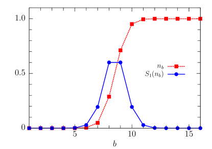
(a) Eigenvalues and entanglement entropy.

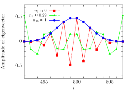
(b) Example eigenvectors.

Figure 1: Fig. 1(a) shows the occupations $n_{b}$ and corresponding entanglement $S_{1}(n_{b})$ from diagonalizing a block of $B=16$ sites in the middle of a system of free gapless fermions on $N=1000$ sites at half filling. The minimum and maximum eigenvalues, $n_{1}$ and $n_{16}$, differ from 0 and 1 by $\approx 1.74\times 10^{-11}$. The eigenvalues closest to 1/2, $1/2-n_{8}=n_{9}-1/2\approx 0.21$, have entropies $S_{1}(n_{8})=S_{1}(n_{9})\approx 0.60$, which are close to the maximum of $S_{1}(1/2)=\log(2)\approx 0.69$. Fig. 4(b) shows examples of eigenvectors from the same diagonalization. The eigenvectors with eigenvalues near 0 and 1, which contribute very little to the entanglement, are localized in the middle of the block, while the eigenvectors with eigenvalues closer to 1/2 which contribute most to the entanglement have large support on the edges of the block.

In our procedure, we will be interested in finding localized eigenvectors of the correlation matrix which are (approximately) fully occupied or unoccupied. By rotating into the basis of these eigenvectors, we can locally diagonalize the correlation matrix, which will lead to a compression of the state. These eigenvectors have eigenvalues near 1 or 0, which makes them (approximate) eigenvectors of the entire correlation matrix and therefore uncorrelated with the rest of the system. What makes it possible to find a localized eigenvector?

The answer is the limited entanglement structure of the states we are interested in (ground states of local Hamiltonians). Consider the entanglement entropy of our fermionic Gaussian state, which can be calculated directly from the correlation matrix. Divide the system into an arbitrary subblock $\mathcal{B}$ of $B$ sites (with the corresponding submatrix of $\Lambda$, which we call $\Lambda_{\mathcal{B}}$) and the rest of the system. We would like to know how large of a block size $B$ we need to find a localized eigenvector. If the matrix $\Lambda_{\mathcal{B}}$ has eigenvalues $\{n_{b}\}$ for $b\in\mathcal{B}$, with $0\leq n_{b}\leq 1$, the entanglement entropy of the subblock $\mathcal{B}$, $S_{B}\equiv-\Tr[\hat{\rho}_{\mathcal{B}}\log(\hat{\rho}_{\mathcal{B}})]$ (where $\hat{\rho}_{\mathcal{B}}$ is the reduced density matrix of the state in subblock $\mathcal{B}$), is

$$S_{B}(\{n_{b}\})=\sum_{b\in\mathcal{B}}S_{1}(n_{b})$$ (6)

where $S_{1}(n_{b})=-[n_{b}\log(n_{b})+(1-n_{b})\log(1-n_{b})]$. This expression has been shown elsewhereLatorre and Riera (2009); Peschel and Eisler (2009); Vidal et al. (2003); Latorre et al. (2004). We show a simple, self contained derivation of it in Appendix A. Note that $S_{1}(n_{b})$ vanishes for both $n_{b}\to 0$ and $n_{b}\to 1$.

The maximum amount of entanglement a block of size $B$ can contain is when $n_{b}=1/2$ for all $b\in\mathcal{B}$, so $S_{B}\leq B\log(2)$. This reflects a volume law entanglement in the “volume” B. However, ground states of 1D local Hamiltonians have entanglement that is much smaller, either of order unity (if the system is gapped), or the entanglement grows as $\log(B)$ if the system is gapless. To avoid the volume entanglement, most of the block eigenvalues $n_{b}$ must be exponentially close to 0 or 1. In other words, as soon as we make $B$ big enough so that the entanglement begins to saturate, except for a possible slow logarithmic growth, we should find at least one eigenvalue very close to 0 or 1. For gapless free fermions in 1D on $N=1000$ sites, we show example eigenvalues, eigenvectors, and corresponding entanglements of a block of $B=16$ in the middle of the correlation matrix in Fig. 1. Even for gapless free Fermions, with a block size of only $B=16$ we find many eigenvalues near 0 or 1 (many localized eigenvectors). We use this observation next to develop algorithms to locally diagonalize correlation matrices and in the process find a very compressed form.

III Algorithms

III.1 Compressing a Correlation Matrix as a GMPS

We begin the procedure by diagonalizing the upper left $B\times B$ subblock of a correlation matrix $\Lambda$ of a pure fermionic Gaussian state. Assume that the state has some local entanglement structure, for example it is the ground state of a local Hamiltonian in 1D. For now, we imagine our system has open boundary conditions. Let $\mathcal{B}$ be the group of sites $1,\ldots B$ on the left end of the system, and $\Lambda_{\mathcal{B}}$ be the associated subblock of $\Lambda$. Also, let $\{n_{b}\}$ be the eigenvalues of $\Lambda_{\mathcal{B}}$ for $b\in\mathcal{B}$ where $0\leq n_{b}\leq 1$. (This constraint on the eigenvalues of the subblock follows from the fact that both $\Lambda$ and $1-\Lambda$ are positive semi-definite.)

We increase $B$ until we find some $n_{b}$ that is nearly 1 or 0 within a specified tolerance, e.g. $10^{-6}$. The closer the eigenvalue is to 1 or 0, the more accurate the compression, but a larger block size translates to more gates and a bigger bond dimension of the MPS we will form. In Fig. 2 we show the most occupied and unoccupied eigenvectors of $\Lambda_{\mathcal{B}}$ for $B=12$ for a system of gapless free fermions in 1D with $N=1024$ sites. We see that $B=12$ is sufficient to give deviations from occupancies of 0 or 1 to nearly machine double precision. The eigenvalues found in the bulk likely will not be as accurate, because states in the bulk will generally be more entangled than the ones on the edge. The smooth fall-off to zero at the right edge of the block is characteristic of these modes and is a result of diagonalizing the block on the left-most boundary of the system. The localized states we find here are least entangled with the rest of the system. This is in contrast to the dominant Schmidt states that are utilized within DMRG which have degrees of freedom that are localized at the edge of the block.

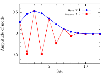
Figure 2: Examples of approximate occupied and unoccupied eigenvectors of $\Lambda$ obtained from diagonalizing $\Lambda_{\mathcal{B}}$ where subblock $\mathcal{B}$ are sites $1,\ldots,B$. $\Lambda$ is formed from the ground state of $\hat{H}=-t\sum_{i=1}^{N-1}(\hat{a}^{\dagger}_{i}\hat{a}_{i+1}+h.c.)$ for $N=1024$ at half filling ($N_{F}=N/2$). A block size of $B=12$ is used. Eigenvectors with highest ($n_{\text{occ}}$) and lowest ($n_{\text{unocc}}$) eigenvalues found from diagonalizing subblock $\mathcal{B}$ are shown. We find $1-n_{\text{occ}}=2.4\times 10^{-15}$ and $n_{\text{unocc}}=7.3\times 10^{-16}$, so the occupations are accurate to nearly machine double precision. $1-n_{\text{occ}}$ and $n_{\text{unocc}}$ should be equal at half filling (because of particle-hole symmetry), but are different in this case as a result of roundoff errors.

The eigenvector $\vec{v}$ which is least entangled is also an approximate eigenvector of the total correlation matrix $\Lambda$, i.e. $\Lambda\vec{v}\approx n_{1}\vec{v}$. Any $N\times N$ unitary matrix that has $\vec{v}$ as its first column represents a change of basis that puts $\vec{v}$ on the first site. The associated transformation of $\Lambda$ will make $\Lambda_{11}=n_{1}$, and zero out the rest of row 1 and column 1. The matrix of eigenvectors of $\Lambda_{\mathcal{B}}$ would produce such a matrix (expanding it to $N\times N$ by putting ones on the diagonal), but this $B\times B$ matrix does not translate well to many-particle gates to use in constructing an MPS.

We now introduce gate/circuit diagrams which apply equally well to simple matrix manipulations of $\Lambda$ and to many-particle tensor networks. The basic ingredient of the diagrams are two site nearest neighbor unitary gates. In Figure 3 we show the relation between a gate and a matrix. In the matrix interpretation, an “MPS” is just a vector with a dimension equal to the number of sites. In a later section we show how a gate is interpreted in the many-particle context of a tensor network. We consider nearest neighbor gates because these translate to fast MPS algorithms—typically, a non-nearest neighbor gate is implemented as a set of swap gates to bring the sites together, a nearest neighbor gate, followed by swaps to return to the original ordering of the sites, which is much slower than a single nearest neighbor gate. In the special case that the intermediate sites are in product states, i.e. bond dimension 1, non-local gates are also inexpensive, and we use these in our MERA algorithm.

Returning to the task of moving the least entangled state $\vec{v}$ to the first site, a set of $B-1$ two-site gates suffices. The first gate acts on sites $(B-1,B)$, and we label it $V_{B-1}$. In general, we take

$$V_{i}=V(\theta_{i})=\begin{pmatrix}\cos\theta_{i}&-\sin\theta_{i}\\ \sin\theta_{i}&\cos\theta_{i}\\ \end{pmatrix}.$$ (7)

We choose $\theta_{B-1}=\tan^{-1}(v_{B}/v_{B-1})$, where $v_{i}$ is the $i^{\text{th}}$ component of the (un)occupied eigenvector of interest $\vec{v}$. With this choice, $V_{B-1}$ acting on $\vec{v}^{T}=\begin{pmatrix}v_{1}&\ldots&v_{B-1}&v_{B}\end{pmatrix}$ sets the last component, $v_{B}$, to zero, and produces a new value of $v_{B-1}\to v^{\prime}_{B-1}$. In other words, we solve for $\theta_{B-1}$ so that $\vec{v}^{T}V_{B-1}=\begin{pmatrix}v_{1}&\ldots&v_{B-1}&v_{B}\end{pmatrix}V_{B-1}=\begin{pmatrix}v_{1}&\ldots&v^{\prime}_{B-1}&0\end{pmatrix}$. Next we rotate sites $(B-2,B-1)$, with $\theta_{B-2}=\tan^{-1}(v^{\prime}_{B-1}/v_{B-2})$, and continue in this fashion. The action of all these gates on $\vec{v}^{T}$ gives $\delta_{i,1}$, so they act to change the basis into the one containing $\vec{v}$.

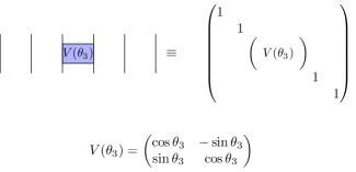
Figure 3: Definition of a gate used throughout the paper. Example for $N=8$ sites for a gate at site $i=4$. Unless specified otherwise, circuits are in a direct sum space. We take the convention that multiplying a matrix from the top by a vector corresponds to multiplying the matrix on the right by a column vector.

We take $V_{\mathcal{B}}=V(\theta_{B-1})V(\theta_{B-2})\ldots V(\theta_{1})$. This procedure is shown schematically for a simple case in Fig. 4(a). We then apply the gates to $\Lambda$. The transformed correlation matrix $V_{\mathcal{B}}^{\dagger}\Lambda V_{\mathcal{B}}$ will have $n_{1}\approx 1$ or $0$ as the top left entry (and nearly 0 in the rest of the entries in the first row and first column). A schematic of this transformation is shown in Fig. 4(b). We will call the first block $\mathcal{B}_{1}\equiv\mathcal{B}$. We repeat this procedure for $\mathcal{B}_{2}$, sites $2,\ldots,B+1$, now simply ignoring the first site. For half-filled systems, the modes found are likely to alternate between occupied and unoccupied because occupied and unoccupied modes will generally be found in pairs when diagonalizing a block of the correlation matrix. Of course, $B$ does not have to stay the same from one block to the next, and in general it is better to set it dynamically to make $n_{k}$ sufficiently close to 1 or 0. For the last blocks, $B$ is decreased to the remaining number of sites. After $N$ blocks, we will have approximately diagonalized $\Lambda$.

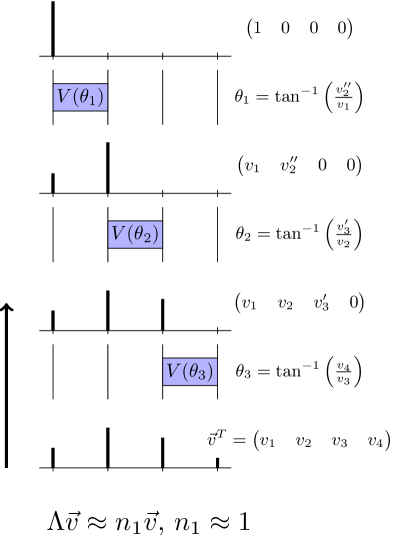
(a)

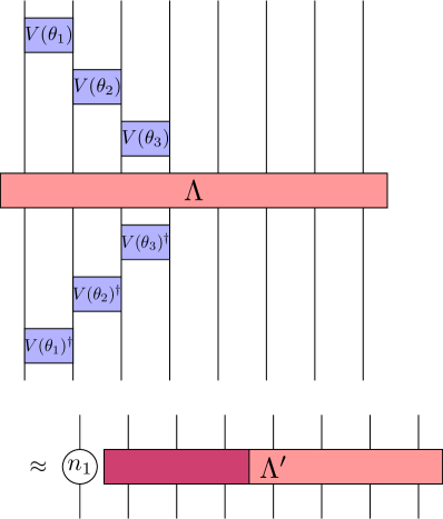
(b)

Figure 4: In Fig. 4(a) we show schematically the procedure to obtain, given an approximate eigenvector $\vec{v}$ of the correlation matrix $\Lambda$, the set of local rotation gates that make up our compressed correlation matrix. The example shown is for a block size $B=4$ and system size $N=8$. Fig. 4(b) shows that, by conjugating the correlation matrix by the gates obtained, the correlation matrix is approximately partially diagonalized.

The overall unitary transformation is $V=V_{\mathcal{B}_{1}}V_{\mathcal{B}_{2}}\ldots V_{\mathcal{B}_{N-1}}$. The matrix $V$ decomposed into the $2\times 2$ rotation gates $\{V(\theta_{i})\}$ for $N=8$ and $B=4$ is shown in Fig. 5(a). The $N\times N$ unitary approximately rotates our single particle basis from real space to what we refer to as the occupation basis, which is one of the highly degenerate eigenbases of the correlation matrix. Conjugating $\Lambda$ by $V$ gives us a matrix $V^{\dagger}\Lambda V$ that is nearly diagonal, with $N_{F}$ values on the diagonal close to 1 corresponding to occupied modes and $N-N_{F}$ values on the diagonal close to 0 corresponding to unoccupied modes. In total, the procedure as described would require $O(BN)$ nearest neighbor rotations, where $B$ is the largest block size needed for the desired accuracy of the representation of the correlation matrix.

(a)

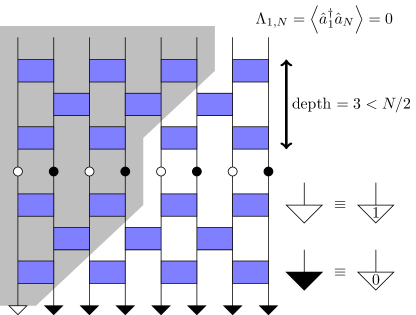
(b)

Figure 5: Fig. 5(a) shows the overall gate structure obtained by the diagonalization procedure. These gates form the total $N\times N$ unitary $V$ which approximately diagonalizes our correlation matrix $\Lambda$. By conjugating a diagonal matrix with the appropriate occupations of 0 or 1 found in the diagonalization procedure by this set of gets, we get an approximation for the correlation matrix. Fig. 5(b) shows an example of the correlations allowed by representing the correlation matrix $\Lambda$ with a diagonal matrix conjugated by a finite depth circuit of depth $<N/2$. The grey area (the “light cone”) represents sites where there can be nonzero correlations with the first site. For this circuit depth, there can’t be correlations with the last two sites. A circuit of depth $\geq N/2$ is required to allow for the possibility of nontrivial correlations across the entire system.

Writing the $2\times 2$ rotations as gates is very convenient for understanding the matrix transformations, but more importantly it makes it easy to connect to many-body gates and to quantum circuits in general. As a quantum circuit, these gates have a slightly peculiar structure. Because of how the diagonalizations overlapped, the circuit has a depth of $O(N)$. However, a vertical cut through the circuit only passes through $O(B)$ gates. This construction and gate structure is in a certain sense optimal if we limit ourselves strictly to circuits with local gates. If we want to represent a correlation matrix in a compact way with nearest neighbor gates, we would like to be able to represent arbitrary correlations in the system (correlations at all lengths), and in particular, correlations between the first and last site. In Fig. 5(b), we show a circuit which cannot connect the first and last sites because its depth is less than $N/2$. Although our gate structure, shown in Fig. 5(a), has a depth $\sim N$, in fact we can adjust our diagonalization procedure slightly to obtain a depth of $\sim N/2$ so our circuit can capture correlations of all lengths. This is done by beginning the diagonalization procedure from both the left and right side of the system until the blocks meet in the middle. This freedom in where to start the diagonalization is similar to the choice of gauge of an MPS. Choosing one gauge over another can be useful if we have already performed this procedure for a correlation matrix and want to perform it again for another correlation matrix which is only locally different from the first one. If we choose the gauge center where the correlation matrix has changed, we only need to change a local set of gates.

A generic local circuit of depth $O(N)$ contains $O(N^{2})$ gates, and can represent an arbitrary $N\times N$ single-particle unitary change of basis. The low entanglement of physical ground states allows us to represent an $N\times N$ matrix with $O(BN)$ one-parameter gates, with $B\ll N$. For a gapless system, we know from conformal field theory that the entanglement of a subblock $\mathcal{B}$ of $B$ sites varies as $S_{B}\sim\log(B)$. This means that we should be able to capture the entanglement of a critical system of $N$ sites with a block size $B\sim\log(N)$. If we find that $B\sim\log(N)$, this means that our construction is roughly optimal. Fig. 14 in Section IV.1 shows numerical evidence that this is indeed the case.

III.2 Compressing a Correlation Matrix as a GMERA

A MERA tensor networkVidal (2007) can represent a 1D critical system using a constant bond dimension, unlike an MPS. In our MPS construction, this is reflected in that $B\sim\log(N)$. However, we can adjust the diagonalization procedure slightly to obtain a MERA-like gate structure with a $B$ which does not grow with $N$. The MERA for fermionic Gaussian states was first studied in Evenbly and Vidal (2010), but was only used to study infinite translationally invariant systems and required a subtle optimization scheme. Here we will show a simpler construction only requiring the tools we have explained so far.

We begin the procedure in the same way as we did for the GMPS, by diagonalizing the block corresponding to sites $1,\ldots,B$ of the correlation matrix. Just as before, for a large enough block size we find an occupied or unoccupied mode and rotate into the basis containing that mode with $B-1$ local $2\times 2$ gates. Next, instead of diagonalizing the block starting at site 2, we instead diagonalize the block corresponding to sites $3,\ldots,B+2$, again finding an occupied or unoccupied mode and rotating into that basis. The state at site 2 is “left behind”—it is not a low entangled state, so we cannot ignore it, but we leave it for a later stage of the algorithm. We continue in this manner, diagonalizing blocks starting at odd sites of size $B$ to obtain $\sim BN/2$ nearest neighbor gates. Approximately half of the modes are fully occupied or unoccupied and are projected out (meaning the associated rows and columns in the correlation matrix are ignored in later stages). The other half were left behind, and continue as the sites of the next layer of the gate structure. By only trying to get $N/2$ unentangled modes in the first layer, the size of $B$ does not need to grow with $N$, as we show below.

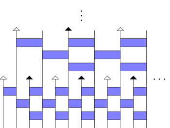
Figure 6: An example of an alternative diagonalization scheme resulting in a MERA-like gate structure. Here we show a section of the first two renormalization steps, with 12 sites shown in the first layer and 6 renormalized sites shown in the second. A block size of $B=4$ is used. For this block size there are two layers of disentanglers and one layer of isometries per level of the MERA.

The left-behind sites pass through to the next layer and are interpreted as a course-grained version of our original state on only $N/2$ sites. We repeat the same procedure for this new course-grained system of $N/2$ sites, starting by diagonalizing the subblock of the first $1,\ldots,B$ sites of the new course-grained lattice, finding an occupied or unoccupied mode of the course-grained system, and projecting it out. Here, however, the gate we use to rotate into the basis of the (un)occupied mode are $2\times 2$ nearest neighbor gates in the course-grained lattice, but are actually next-nearest neighbor gates acting on the original lattice (if we project out every other site). Ordinarily, using next-nearest neighbor gates (or longer range gates at higher levels of the MERA) would be costly in the many-body case, requiring swap gates to make them effectively nearest neighbor. However, the projected-out sites are now in product states, meaning that swapping does not require significant time.

We repeat the above procedure of projecting out every other effective site and course graining to a lattice of half the size. All of the sites will be projected out after this course-graining is repeated $O(\log_{2}(N))$ times. Fig. 6 shows the first two layers of the resulting gate structure, which looks like a MERA with $B-2$ layers of nearest neighbor 2-site disentanglers and a layer of nearest neighbor 2-site isometries. The total number of gates in the construction is $\sim B(N/2+N/4+\ldots+1)=BN$, the same gate count for a fixed block size $B$ as for the GMPS. We call this gate structure, which like our GMPS construction is a compression of an $N\times N$ correlation matrix into $\sim BN$ gates, a fermionic Gaussian MERA or GMERA. In this figure, triangles denote projections onto the appropriate occupation found. These are the modes that are uncorrelated with the rest of the sites and can be ignored in the next layer. Some extra gates will be required to project out the leftover sites at the right end of the system (not shown in Fig. 6), and there is some flexibility in how to do this which will change the accuracy of the compression slightly. For example, one could use a gate structure similar to the GMPS construction to project out all of the leftover sites at the end.

How does the block size $B$ of the GMERA compare to that in our GMPS construction? We show numerically in Section IV.2 that for a simple gapless Hamiltonian the GMERA does indeed produce accurate results with a block size $B=O(1)$, independent of the system size, making it much more efficient in the large $N$ limit.

III.3 Discrete Wavelet Transforms and Fermionic Gaussian MERA

We would like to point out the similarity between the MERA gate structure and orthogonal wavelet transforms (WT), such as the WTs that produce the well-known Daubechies wavelets Daubechies (1988); Daubechies et al. (1992). Of course, the development of wavelets has not been in a many particle context, and, for now, we restrict ourselves to the matrix interpretation of the diagrams. For compact wavelets, an orthogonal wavelet transform is a local unitary transformation. It is not usually represented in terms of two-site gates, but this representation turns out be be particularly convenient. To be specific, we start with the simplest nontrivial WT, the D4 Daubechies WT. This WT is defined by four coefficients $\{a_{j}\}$ for $j=1,\ldots,4$ which characterize how the D4 scaling function is related to itself at different scales through the equation $s(x)=\sum_{j}a_{j}\sqrt{2}s(2x-j)$. The matrix form of the WT is given by

$$\begin{pmatrix}a_{1}&a_{2}&a_{3}&a_{4}&0&0&0&\\ a_{4}&-a_{3}&a_{2}&-a_{1}&0&0&0&\\ 0&0&a_{1}&a_{2}&a_{3}&a_{4}&0&\\ 0&0&a_{4}&-a_{3}&a_{2}&-a_{1}&0&\\ &&&&&&&&\ddots\\ \end{pmatrix}.$$ (8)

The $\{a_{j}\}$ are carefully chosen to ensure orthogonality between scaling functions centered at different sites, and to make the scaling functions have desirable completeness properties. For example, linear combinations of the D4 scaling functions centered at different sites, $\{s(x-k)\}$ for integer $k$, fit any linear function, so the resulting coefficients are $\vec{a}^{T}=(1+\sqrt{3},3+\sqrt{3},3-\sqrt{3},1-\sqrt{3})/(4\sqrt{2})$. The orthogonality requirement results in nonlinear equations to solve for the $\{a_{j}\}$ which becomes complicated for higher order. The second row of the matrix gives the coefficients that produces wavelets, designed to represent high momentum degrees of freedom. In terms of our MERA procedure, the wavelets are left behind, while the scaling functions propagate to the next level.

The D4 WT has a very simple gate structure, identical to our MERA structure with $B=3$, shown for two layers in Fig. 7. In each horizontal layer of gates, all gates have the same angle. The D4 WT is specified by only two angles, $\theta_{1}$ for the bottom layer and $\theta_{2}$ for the next. Higher order WTs of this type (e.g. D6, D8, etc.) correspond to larger $B$. (For example, the D6 WT looks like Fig. 6). Given the angles, one gets the $\{a_{j}\}$ by setting all the top values of the circuit to zero except a 1 on one site and applying the $2\times 2$ rotations in the layers below. The support of the scaling functions is made obvious using the gate structure, as there will be $2L$ nonzero values at the bottom of the circuit for $L$ layers of gates. For the D4 WT, one finds that $\theta_{1}=\pi/6$ and $\theta_{2}=5\pi/12$ reproduces the D4 $\{a_{j}\}$, up to a trivial reversal of the coefficients. (A single layer with $\theta_{1}=\pi/4$ gives the trivial Haar wavelets, which have been used previously as a basis for transforming fermionic Gaussian states by Qi Qi (2013).) The scaling functions at the larger scales are found by performing the same transformation of $L$ layers of gates on the scaling functions found at the previous scale.

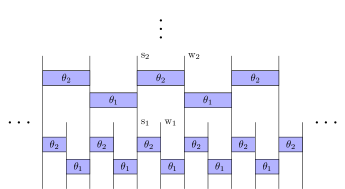
Figure 7: Here we show an example of a discrete wavelet transform written in the gate notation introduced in this paper. We show the D4 wavelet, which corresponds to a fermionic Gaussian MERA with one layer of disentanglers and one layer of isometries per layer. w₁ and s₁ (w₂ and s₂) label wavelet and scaling functions for the first (second) layer. Taking $\theta_{1}=\pi/6$ and $\theta_{2}=5\pi/12$, we reproduce the conventional scaling coefficients for the D4 WT, $\vec{a}^{T}=(a_{1},a_{2},a_{3},a_{4})=(1+\sqrt{3},3+\sqrt{3},3-\sqrt{3},1-\sqrt{3})/(4\sqrt{2})$.

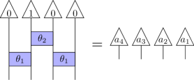
(a) Scaling coefficients from gate structure.

(b) Gate structure in (a) written in terms of matrices and vectors.

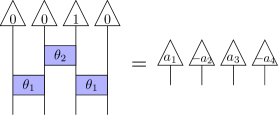
(c) Wavelet coefficients from gate structure.

Figure 8: Here we show explicitly how to obtain the scaling and wavelet coefficients of the D4 WT from the circuit construction. Taking $\theta_{1}=\pi/6$ and $\theta_{2}=5\pi/12$, in (a) and (b) we reproduce the conventional scaling coefficients for the D4 WT, $\vec{a}^{T}=(a_{1},a_{2},a_{3},a_{4})=(1+\sqrt{3},3+\sqrt{3},3-\sqrt{3},1-\sqrt{3})/(4\sqrt{2})$, up to a trivial reversal in the order. In (c) with the same choice of angles we reproduce the conventional wavelet coefficients $(a_{4},-a_{3},a_{2},-a_{1})$, again up to a trivial reversal and sign.

In Fig. 8 we show how scaling coefficients $\{a_{j}\}$ come from the gate structure, applying a vector to the top of the circuit with 1 at the site of a scaling function and 0’s elsewhere. In simple wavelet treatments, the wavelet coefficients are obtained from the scaling coefficients $\{a_{j}\}$ as $\{(-1)^{j-1}a_{2L-j+1}\}$ for $j=1,\ldots,2L$. Here, they are obtained by shifting the location of the 1 at the top of the circuit, but we can show in general that this gives the same result. This is done by noting that the shift of the 1 to get the wavelet coefficients looks like a swap at the top of the circuit. We can “pull through” this swap by conjugating each layer of the WT with a transformation that reverses the order of the sites. This conjugation also negates the angles in the circuit. It leaves a site reversal at the bottom of the circuit, reversing the order of the coefficients. The angle negation negates the sine terms, leading to the same coefficients except with every other one negated, since every other site will have an even or odd number of $\sin(\theta_{i})$ multiplied together.

Given an arbitrary set of $\{a_{j}\}$, we can use the same procedure that brought $\vec{v}$ to the first site in our GMPS procedure to find all the angles defining the WT, i.e $\vec{v}=\vec{a}$. Thus, any compact orthogonal WT of this general type can be represent by a simple gate structure. Because wavelets are much easier to understand than generic many particle wavefunctions, the connection between MERA and wavelets may help provide intuition that helps one understand MERA.

III.4 Forming the Many-Body MPS from the GMPS (or GMERA)

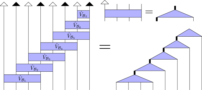
Figure 9: Tensor diagram showing the structure of gates $\{\hat{V}_{\mathcal{B}_{i}}\}$ for $i=1,\ldots,N-1$ obtained in our procedure and how they contract to form an MPS. Here we show a system with $N=8$ sites and a block size $B=4$. The diagram on the right shows that once the sites are rotated into a basis where one of the modes is occupied or unoccupied (generally with some alternating pattern), the fully occupied or unoccupied modes can be projected out. The transformations $\{\hat{V}_{\mathcal{B}_{i}}\}$, including the projections, can be directly interpreted as the tensors composing the MPS representation of our many-body state if we do an exact contraction, or we can apply them as a set of gates as explained in the text.

For a number conserving real Hamiltonian $H$, the many particle unitary gate $\hat{V}_{i}$ corresponding to the single particle rotation $V_{i}$, in the basis $\{\ket{\Omega},\hat{a}^{\dagger}_{i}\ket{\Omega},\hat{a}^{\dagger}_{i+1}\ket{\Omega},\hat{a}^{\dagger}_{i}\hat{a}^{\dagger}_{i+1}\ket{\Omega}\}$, is

$$[\hat{V}_{i}]=[\hat{V}(\theta_{i})]=\begin{pmatrix}1&0&0&0\\ 0&\cos\theta_{i}&\sin\theta_{i}&0\\ 0&-\sin\theta_{i}&\cos\theta_{i}&0\\ 0&0&0&1\\ \end{pmatrix}.$$ (9)

This reinterpretation of the gates is the only change need to make our matrix gate structures act on the many particle Hilbert space.

Say we have compressed the correlation matrix of a pure fermionic Gaussian state as a GMPS. To create the MPS representation of this state, we begin with a product state, with each site being occupied or unoccupied, with the occupations given by $n_{k}$ obtained in our diagonalization procedure (set to 1 or 0 for $n_{k}\approx 1$ or 0). We then apply, one by one, all of the nearest neighbor gates $\{\hat{V}_{i}\}$ (the many-body gates corresponding to the gates $\{V_{i}\}$ obtained with Eq. 9) in the opposite order in which they were obtained with our diagonalization procedure. The repeated application of gates is similar to the time-evolving block decimation (TEBD) algorithmVidal (2004) or the time dependent DMRG algorithmWhite and Feiguin (2004), but the pattern of gates and ordering is different. We apply the two body gates by moving the center of the MPS to the location of the gate, contract the gate with the two relevant tensors in the MPS, and then form the new MPS by performing a singular value decomposition (SVD), with possible truncation of states by throwing out states with small singular values.

We can also form the MPS from our GMERA construction in a similar manner. However, instead of starting with a full product state, we start with the gates at the top of the MERA and work our way down, including only the sites that have been touched by a gate at that level or above. When a site is added, it starts as a completely occupied or unoccupied state, and is immediately mixed with another site by a gate. The number of sites involved roughly doubles with each layer, and after $O(\log_{2}(N))$ layers of the MERA we have our MPS approximation for the entire system. Again, we can truncate as needed by throwing out low weight states after the SVD as we work our way down.

Returning to the MPS construction, the tensors of the MPS could also be constructed directly by contractions of the gates as shown in Fig. 9. In this diagram the small black and white triangles signify projectors onto the appropriate occupations found, while the thick lines signify combined internal indices which form the internal bonds of the MPS. From this perspective it is easy to see that picking a block size $B$ for diagonalizing the correlation matrix would correspond to an MPS with a bond dimension of $\chi=2^{B-1}$. We find it simpler and more efficient to apply the gates layer by layer instead of this method. Layer by layer, it is natural to truncate the MPS with SVDs during the construction, and this can lead to an MPS with a smaller bond dimension than $2^{B-1}$ for the required accuracy. The SVD truncation takes one out of the manifold of Gaussian states, where the greater freedom for a fixed bond dimension allows one to find a state which is closer to the desired Gaussian state than one could within the Gaussian manifold. However, one should pick a block size so that $2^{B-1}$ is as close to the target bond dimension as possible.

We can adapt our circuits to complex quadratic Hamiltonians, where the gates are of the same form but the $2\times 2$ submatrix rotating the singly occupied subspace is a general matrix in SU(2) parameterized by two angles. Even more generally, we can extend this procedure to quadratic Hamiltonians with pairing terms to compress BCS states, where the gates required are not just number conserving but general parity conserving gates (so they involve mixing of unoccupied and doubly occupied subspaces of the 2 sites of interest). This matrix would in general be parameterized by 5 angles (one matrix in SU(2) rotating the singly occupied subspace, one matrix in SU(2) rotating the empty and doubly occupied subspaces, and a relative phase). This form of gates has been studied previously in the context of classically simulating quantum circuits using the matchgate formalism; see for exampleValiant (2002); Jozsa and Miyake (2008).

IV Numerical Results

Here we show numerical results for the algorithms we presented. In order to study systems that are both gapless and gapped, we study a simple model, the Su-Schrieffer-Heeger model Su et al. (1979). This is a model of 1D spinless fermions hopping on a lattice with staggered hopping amplitudes, $t_{1}$ and $t_{2}$. The Hamiltonian is

$$\hat{H}_{SSH}=\sum_{i=1}^{\frac{N-1}{2}}(t_{1}\hat{a}_{2i-1}^{\dagger}\hat{a}_{2i}+t_{2}\hat{a}_{2i}^{\dagger}\hat{a}_{2i+1}+h.c.).$$ (10)

We will take $t_{1}=-t\left(1+\frac{\delta}{2}\right)$ and $t_{2}=-t\left(1-\frac{\delta}{2}\right)$. The model has an energy gap in the bulk between the ground state and first excited state of $\Delta=2|\delta|t$ in the thermodynamic limit ($N\rightarrow\infty$). With open boundary conditions, it can contain exponentially decaying zero energy modes localized on the ends of the chain.

IV.1 Results for Compressing a Correlation Matrix as a GMPS

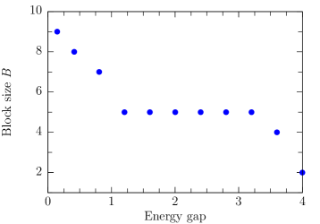
Figure 10: Block size required to obtain a relative error in the total energy of less than $10^{-6}$ as a function of the calculated energy gap (in units of $t$) for $N=128$ sites.

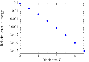
Figure 11: Relative error in the total energy as a function of the block size $B$ for $N=128$ sites and $\delta=0$.

We start with a simple test of obtaining the GMPS compression of the ground state correlation matrix of the SSH model for $N=128$ lattice sites for various energy gaps at half filling ($N_{F}=N/2$). We analyze the range of $\delta$ from 0 to $2$. The ground state for $\delta=0$ is (approximately) gapless while for $\delta=2$ it is fully gapped (the chain uncouples). Fig. 10 shows the block size required to obtain a GMPS with a relative error in the total energy of less than $10^{-6}$ as a function of the calculated energy gap. The exact ground state energy and energy gap are calculated by diagonalizing the hopping Hamiltonian $H_{SSH}$. This corresponds to the accuracy of the MPS representation of the ground state if the GMPS written with many-body gates is contracted with no further truncation of the MPS, so a GMPS block size $B$ corresponds to an MPS of bond dimension $\chi=2^{B-1}$ (which is why the block size remains constant for intermediate energy gaps). The plot shows, as expected, that the block size required decreases as the energy gap is increased. Fig. 11 shows, for the case $\delta=0$ (where the energy gap, due to the finite size, is 0.146088$t$), the relative error in the energy as a function of the block size.

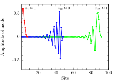
(a) $\delta=0.4$ (energy gap $\approx 0.806135t$)

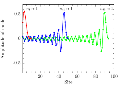
(b) $\delta=0$ (energy gap $\approx 0.146088t$)

Figure 12: Examples of occupied and unoccupied modes found in the diagonalization process. Fig. 12(a) shows occupied/unoccupied modes for $\delta=0.4$ (energy gap $\approx 0.806135t$). Fig. 12(b) shows occupied/unoccupied modes for $\delta=0$ (energy gap $\approx 0.146088$).

(a) $\delta=0.4$ (energy gap $\approx 0.806135t$)

(b) $\delta=0$ (energy gap $\approx 0.146088t$)

Figure 13: Examples of deviations in occupations at the end of the diagonalization procedure for $N=128$ sites. Fig. 13(a) shows errors in the occupations for $\delta=0.4$ (energy gap $\approx 0.806135t$). Fig. 13(b) shows errors in the occupations for $\delta=0.0$ (energy gap $\approx 0.146088t$).

Fig. 12 shows examples of the modes obtained with the procedure, both filled and unfilled, for a small gap and a larger gap. The modes are seen to be localized for the case of the larger gap, and extend throughout the system for the smaller gap. The unfilled modes follow the same decay as the filled modes but oscillate more, since they are above the Fermi sea and are therefore higher in energy. Fig. 13 shows for the same two gaps the deviation in the eigenvalues $n_{k}$ from 0 or 1 obtained during the diagonalization procedure. For the case of the larger gap, this error saturates to its maximum quickly for modes near the middle of the system, while for the smaller gap, the error increases more slowly due to the longer range correlations.

Figure 14: Block size $B$ needed for a relative error in the energy of $<10^{-6}$ as a function of number of sites $N$ for spinless, gapless fermions with open boundary conditions at half filling. As expected from arguments about the entanglement of a critical system, we find $B\sim\log(N)$, tested up to $N=2^{16}=65536$ sites (note the $\log$ scale on the x axis). To study systems of this size and avoid the $O(N^{3})$ diagonalization of the hopping Hamiltonian, we obtain the correlation matrix using the GDMRG algorithm as explained in Appendix B.

In Fig. 14 we analyze the block size scaling with system size $N$ for the gapless case ($\delta=0$). As we expect from arguments about entanglement made at the end of Section III.1, the scaling is found to be $B\sim\log(N)$. This is the expected scaling for a critical 1D system. We can see that with this procedure we can analyze very large systems, up to $N=2^{16}=65536$ sites, even for gapless free fermions. To avoid storing correlation matrices this large, we begin with a very accurate compressed correlation matrix as a GMPS using the GDMRG algorithm presented in Appendix B. With GDMRG, we begin with a state with a relative error in the energy of $<10^{-10}$. For $N=65536$ this requires a block size of $B=22$. We then obtain the local correlation matrix for the block we are interested in using the gates from this accurate compression, and use it to obtain a less accurate compression with a smaller block size. This procedure should lead to, for a given block size, a more accurate overall state than one that would be obtained directly from GDMRG, because GDMRG optimizes the energy which only depends on very local correlations.

IV.2 GMERA Results

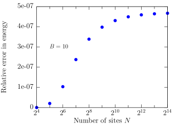
Figure 15: Relative error in the energy for the proposed GMERA construction for increasing number of sites for a block size $B=10$. The system analyzed is the ground state of free fermions hopping on a lattice with open boundary conditions. All errors are below $10^{-6}$. As expected for a MERA, the error is seen to saturate for large $N$, indicating a fixed block size is sufficient to obtain an accuracy $<10^{-6}$ up to very large system sizes.

Here we present results for compressing a correlation matrix as a GMERA using the procedure presented in Section III.2. We show the relative error in the energy for increasing number of sites for $B=10$ in Fig. 15. We see that for this block size, the error stays below $10^{-6}$ for systems up to $N=2^{14}=16384$ and in fact appears to saturate at high number of sites (the change in the relative error in the energy approaches 0 for larger system sizes). This is in stark contrast to the GMPS, where a block size $B\sim\log(N)$ was required to obtain a fixed accuracy, as shown in Fig. 14. Instead, the GMERA obtains the same accuracy with constant block size $B$ as shown in Fig. 15. The GMPS obtains the given accuracy with the same or smaller block size up to $N=512$, after which it requires a larger block size than the GMERA to obtain the same level of accuracy. As we mentioned earlier, this is made possible partially because the GMERA structure involves nonlocal gates.

IV.3 GMPS to Many-Body MPS Results

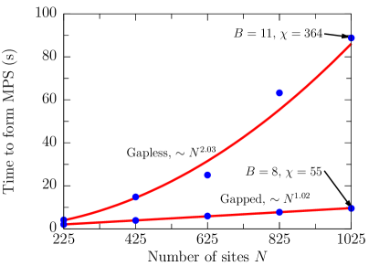
Figure 16: A plot of the time to form the MPS approximation of gapped and gapless free fermion ground states at half filling as a function of sites $N$ using gates from a GMPS. The bond dimensions are chosen large enough such that the relative errors in the energy of the MPS are below $10^{-6}$. The block size of the GMPS used to form the MPS are the minimum required to obtain a GMPS with a relative error in the energy of $10^{-6}$. A cutoff in the singular values of the SVD of $10^{-11}$ was used when applying the gates to form the MPS using the method described in Section III.4. For the gapped case, the SSH model with $\delta=0.1$ is used, corresponding to an energy gap of $\Delta\approx 0.2t$ (exact as $N\rightarrow\infty$).

Plots of the time it takes to form the MPS of the ground state of a gapless free fermion system for up to $N=1024$ sites using the method presented in Section III.4 are shown in Fig. 16. As expected, the time it takes for a gapless system is polynomial in the system size $N$, while it is approximately linear in $N$ for a gapped system. The SSH model is used with $\delta=0.1$ or an energy gap $\Delta\approx 0.2t$. The time to form the gapless ground state is only a modest polynomial in $N$, $\sim N^{2.03}$, while as we expect from arguments about entanglement the time to form the gapped ground state is very nearly linear in $N$, $\sim N^{1.02}$, because the block size and bond dimension required to obtain the specified accuracy are constant for all $N$ shown ($B=8$ and $\chi=55$). With this method, a gapless ground state of $N=1025$ sites with a relative error in the energy of $<10^{-6}$ can be formed on a laptop in only $\sim 90$ seconds.

An interesting point to emphasize is the quality of the compression. The GMPS for the gapless ground state on $N=1025$ sites requires a block size of $B=11$ to obtain a relative error in the energy of $<10^{-6}$. Naively, turning these gates into many-body gates and contracting the network (forming the MPS directly from the GMPS with no truncation) as explained earlier leads to a bond dimension of the MPS of $\chi=2^{B-1}=2^{10}=1024$. However, applying the gates as described and using a cutoff of the singular values of $10^{-11}$ leads to the formation of an MPS approximation of the fermionic Gaussian ground state, still with a relative error in the energy of $<10^{-6}$, with a bond dimension of only $\chi=364$. This is a result of the fact that our GMPS only explores the manifold of fermionic Gaussian states limited to the specified block size. On the other hand, the MPS approximation of the Gaussian state we form from this GMPS is able to explore the entire manifold of MPS’s up to the allowed bond dimension (and particle number if symmetric tensors are used, as we do here), so through the SVD we are able to compress the state quite efficiently beyond what we initially might expect.

V Conclusion

We have presented an efficient, numerically stable, and controllably accurate way to compress a correlation matrix into a set of $2\times 2$ unitary gates. From these gates, we have also presented a method for easily and efficiently forming the MPS approximation of a fermionic Gaussian state. We explained the procedure in detail for the ground state of a generic number conserving Hamiltonian. We then presented results for the SSH model, a 1D chain of fermions with staggered hopping. We showed examples of the accuracy and block sizes needed for different gaps of the model. We hope this method can be used as a simple, efficient and reliable procedure for directly preparing many states of interest, either by creating starting states to aid DMRG calculations or preparing a particular ansatz as an MPS. We also presented one example of how the procedure can be modified to obtain different gate structures, in this case one that is related to the MERA. However, there are other possibilities to be explored, such as gate structures more directly suited for systems with 2 spatial dimensions, periodic boundary conditions, as well as how the method might be applied to study thermal fermionic Gaussian states. In addition, we presented how discrete wavelet transforms can be described very simply with the gate structure notation we introduced in this paper.

The method is easily generalized to cases beyond the one presented here. As we touched upon earlier, it can be generalized to the case of BCS states, the ground states of hopping Hamiltonians that include pairing terms. In this case, the correlation matrix in the Majorana basis can be written in terms of an anti-symmetric matrix which can be approximately block diagonalized by $\sim 5BN$ local $2\times 2$ rotation gates, which are turned into nearest neighbor parity-conserving many-body gates. The case of spinless fermions was presented, but spinful fermions are a simple generalization.

Appendix A Calculation of the Entanglement Entropy of a Fermionic Gaussian State

In this section we give a simple, self-contained derivation for Eq. 6, the entanglement entropy for a block of a free fermion system. Assume the block of interest $\mathcal{B}$ is the first $B$ sites.

Gaussian states have expectation values that obey Wick’s theorem. This means that the expectation value of any operator contained within the block is specified if we know subblock $\mathcal{B}$ of the correlation matrix, $\Lambda_{\mathcal{B}}$. This implies that the many-body density matrix of the block $\hat{\rho}_{\mathcal{B}}$ is also uniquely specified by $\Lambda_{\mathcal{B}}$. The entanglement entropy on block $\mathcal{B}$, defined as $S_{B}[\hat{\rho}_{\mathcal{B}}]=-\Tr[\hat{\rho}_{\mathcal{B}}\log(\hat{\rho}_{\mathcal{B}})]$, does not change under general unitary transformations within the block. Thus, we can perform the single particle unitary transformation of basis that makes $\Lambda_{\mathcal{B}}$ diagonal, with diagonal entries $n_{b}=\left<\hat{a}^{\dagger}_{b}\hat{a}_{b}\right>$ for $b\in 1,\ldots,B$. The $n_{b}$ uniquely specify the reduced density matrix of the block, so the entanglement is a universal function of $\{n_{b}\}$:

$$S_{B}=S_{B}(n_{1},\ldots,n_{B}).$$ (11)

In fact, the details of the system outside the block are irrelevant. For example, different systems with different numbers of sites outside the block can have the same $S_{B}$ as long as their $\{n_{b}\}$ are identical and the system is a Gaussian state. Thus to evaluate the function $S_{B}$, we can choose a simple system in which to evaluate it rather than using the actual system of interest.

Let’s first consider a block with only one site ($B=1$). We would like to know the universal function $S_{1}(n_{1})$. We choose a two site system containing a single particle, with normalized wavefunction

$$\ket{\psi}=(\sqrt{n_{1}}\hat{a}^{\dagger}_{1}+\sqrt{1-n_{1}}\hat{a}^{\dagger}_{2})\ket{\Omega}.$$ (12)

The correlation matrix is

$$\begin{pmatrix}n_{1}&\sqrt{n_{1}(1-n_{1})}\\ \sqrt{n_{1}(1-n_{1})}&1-n_{1}\end{pmatrix}$$ (13)

which has the required block correlation matrix $\Lambda_{1}=(n_{1})$. The Schmidt decomposition of $\ket{\psi}$ is

$$\begin{aligned} \ket{\psi}&=\sqrt{1-n_{1}}(\ket{0})(\hat{a}^{\dagger}_{2}\ket{0})+\sqrt{n_{1}}(\hat{a}^{\dagger}_{1}\ket{0})(\ket{0})\\ &=\sqrt{1-n_{1}}\ket{0}\ket{1}+\sqrt{n_{1}}\ket{1}\ket{0}\end{aligned}$$ (14)

where $\ket{1}$ is the occupied state of the corresponding site. From this we see that the reduced density matrix for site 1, $\hat{\rho}_{1}=\Tr_{2}[\ket{\psi}\bra{\psi}]$, is

$$\begin{aligned} \hat{\rho}_{1}&=(1-n_{1})\ket{0}\bra{0}+n_{1}\ket{1}\bra{1}\\ &=(1-n_{1})(\hat{I}_{1}-\hat{n}_{1})+n_{1}\hat{n}_{1}\end{aligned}$$ (15)

and

$$\begin{aligned} S_{1}(n_{1})&=-\Tr[\hat{\rho}_{1}\log(\hat{\rho}_{1})]\\ &=-(1-n_{1})\log(1-n_{1})-n_{1}\log(n_{1}).\end{aligned}$$ (16)

For the system $\mathcal{B}$ with block size $B>1$, we can choose the system to be of size $2B$ and for each site in the block associate one site outside the block. The Gaussian state is the product state of the single particle states living on a pair, each identical in form to the $B=1$ state, with $B$ total particles. This system has no correlations or entanglement between these pairs. This means that the entanglement is the sum of the entanglement of each pair. Thus

$$S_{B}(\{n_{b}\})=\sum_{b\in\mathcal{B}}S_{1}(n_{b})$$ (17)

which is identical to Eq. 6. Note also that the overall reduced density matrix of the block is the product of the single site density matrices given in Eq. 15.

An alternative argument can be made to derive the same equation which avoids the introduction of a contrived environment. We could have taken as an ansatz that the reduced density matrix on $\mathcal{B}$, $\hat{\rho}_{\mathcal{B}}$, is the product of the single site reduced density matrix we derived in Eq. 15, in other words $\hat{\rho}_{\mathcal{B}}=\otimes_{b\in\mathcal{B}}\hat{\rho}_{b}$. We can show that this is in fact the unique reduced density of the state we are interested in if we can show that it reproduces the correct correlation matrix of our state and is a fermionic Gaussian state (that it obeys Wick’s theorem). Both of these are easy to show explicitly. Once we verify that this is indeed the correct reduced density matrix of our state, we can calculate the entanglement entropy directly with $S_{B}=-\Tr[\hat{\rho}_{\mathcal{B}}\log(\hat{\rho}_{\mathcal{B}})]=-\sum_{b\in\mathcal{B}}\Tr[\hat{\rho}_{b}\log(\hat{\rho}_{b})]$, which matches Eq. 6.

Appendix B GDMRG, an Algorithm to Obtain a Compressed Ground State Correlation Matrix as a GMPS

Here we describe fermionic Gaussian DMRG (GDMRG), a DMRG-like algorithm in the single particle context. The algorithm is an efficient method to directly obtain all the angles specifying the compressed correlation matrix as a GMPS without ever needing to express the matrix in uncompressed form. The ground state GMPS of a hopping Hamiltonian on $N$ sites is calculated with a cost of only $O(B^{3}N)$, where $B$ is the block size of the GMPS (which determines the accuracy of the compression and depends on the entanglement of the ground state).

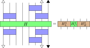
(a)

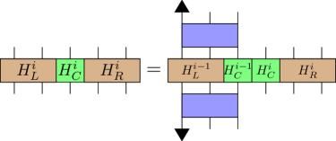
(b)

Figure 17: Fig. 17(a) shows an example of an effective Hamiltonian centered at site 4 for the GDMRG algorithm. The example is for $N=8$ sites and a block size of $B=3$. Here the center is only one site, but could be more to improve convergence just like in the standard DMRG algorithm. Fig. 17(b) shows, for a sweep to the right, how to obtain the new left block from the previous effective Hamiltonian.

Imagine that we start with a hopping Hamiltonian $H$ on a lattice of $N$ sites, and we would like to obtain the GMPS with a block size $B$ that minimizes the energy of $H$. We begin with a random starting GMPS. Just like in the DMRG algorithm, we form an effective Hamiltonian centered at a site with a left and right block, which we show in Fig. 17(a). Say that we start on the left side of the lattice and begin sweeping right. Our GMPS will start gauged to the left. For a single-site GDMRG, our center block is only one site, but we could use a larger center to decrease the number of sweeps required for convergence. In practice for free gapless fermions we find that a single center site works quite well. The first step is to diagonalize the $2B-1$ site effective Hamiltonian, and obtain the effective correlation matrix $\Lambda_{\text{eff}}$. Using this $\Lambda_{\text{eff}}$, we diagonalize the first $B\times B$ block and, for a large enough $B$, find a fully occupied or unoccupied mode. Just as described in Fig. 4, we find the $B-1$ nearest neighbor $2\times 2$ gates that rotate $\Lambda_{\text{eff}}$ into the basis containing this mode, partially diagonalizing it. These gates form the first block of the GMPS.

Next we would like to move the center to the right so that we can obtain the next block of the GMPS. Because the compression is a unitary transformation, we can start moving the center to the right by undoing the gates in the block of the GMPS to the right of the center. This is step is in contrast to ordinary DMRG where a sequence of right blocks are stored and are called from memory when needed. We then obtain the effective Hamiltonian for the next site using the block of the GMPS we obtained from the previous effective Hamiltonian of the sweep, as shown in Fig. 17(b). We repeat this process until we reach the end of the lattice, completing our first sweep. We continue sweeping back and forth until the energy is sufficiently converged. We use this algorithm to obtain a very accurate correlation matrix for systems up to $N=2^{16}=65536$, from which we obtain the GMPS in Fig. 14. For $N=65536$ sites to obtain a correlation matrix with a relative error in the energy of less than $10^{-10}$, we require a block size of $B=22$ and 14 sweeps (where a single sweep is from left to right or right to left).

References

- White (1992) S. R. White, Phys. Rev. Lett. 69, 2863 (1992).
- White (1993) S. White, Phys. Rev. B 48, 10345 (1993).
- Gutzwiller (1963) M. C. Gutzwiller, Physical Review Letters 10, 159 (1963).
- Zhang et al. (1995) S. Zhang, J. Carlson, and J. E. Gubernatis, Phys. Rev. Lett. 74, 3652 (1995).
- Zhang et al. (1997) S. Zhang, J. Carlson, and J. E. Gubernatis, Phys. Rev. B 55, 7464 (1997).
- Evenbly and Vidal (2010) G. Evenbly and G. Vidal, Phys. Rev. B 81, 235102 (2010).
- Kraus et al. (2010) C. V. Kraus, N. Schuch, F. Verstraete, and J. I. Cirac, Phys. Rev. A 81, 052338 (2010).
- Latorre and Riera (2009) J. I. Latorre and A. Riera, Journal of Physics A: Mathematical and Theoretical 42, 504002 (2009).
- Peschel and Eisler (2009) I. Peschel and V. Eisler, Journal of Physics A: Mathematical and Theoretical 42, 504003 (2009).
- Vidal et al. (2003) G. Vidal, J. I. Latorre, E. Rico, and A. Kitaev, Phys. Rev. Lett. 90, 227902 (2003).
- Latorre et al. (2004) J. Latorre, E. Rico, and G. Vidal, Quant.Inf.Comput. 4, 48 (2004), arXiv:quant-ph/0304098 [quant-ph] .
- Vidal (2007) G. Vidal, Phys. Rev. Lett. 99, 220405 (2007).
- Daubechies (1988) I. Daubechies, Communications on pure and applied mathematics 41, 909 (1988).
- Daubechies et al. (1992) I. Daubechies et al., Ten lectures on wavelets, Vol. 61 (SIAM, 1992).
- Qi (2013) X.-L. Qi, arXiv:1309.6282 (2013).
- Vidal (2004) G. Vidal, Phys. Rev. Lett. 93, 040502 (2004).
- White and Feiguin (2004) S. White and A. Feiguin, Phys. Rev. Lett. 93, 076401 (2004).
- Valiant (2002) L. G. Valiant, SIAM Journal on Computing 31, 1229 (2002), http://dx.doi.org/10.1137/S0097539700377025 .
- Jozsa and Miyake (2008) R. Jozsa and A. Miyake, Proceedings of the Royal Society A: Mathematical, Physical and Engineering Science 464, 3089 (2008).
- Su et al. (1979) W. P. Su, J. R. Schrieffer, and A. J. Heeger, Phys. Rev. Lett. 42, 1698 (1979).