Reconstructing the inflaton potential from the spectral index

Abstract

Recent cosmological observations are in good agreement with the scalar spectral index $n_{s}$ with $n_{s}-1\sim-2/N$, where $N$ is the number of e-foldings. Quadratic chaotic model, Starobinsky model and Higgs inflation or $\alpha$-attractors connecting them are typical examples predicting such a relation. We consider the problem in the opposite: given $n_{s}$ as a function of $N$, what is the inflaton potential $V(\phi)$. We find that for $n_{s}-1=-2/N$, $V(\phi)$ is either $\tanh^{2}(\gamma\phi/2)$ (”T-model”) or $\phi^{2}$ (chaotic inflation) to the leading order in the slow-roll approximation. $\gamma$ is the ratio of $1/V$ at $N\rightarrow\infty$ to the slope of $1/V$ at a finite $N$ and is related to ”$\alpha$” in the $\alpha$-attractors by $\gamma^{2}=2/3\alpha$. The tensor-to-scalar ratio $r$ is $r=8/N(\gamma^{2}N+1)$. The implications for the reheating temperature are also discussed. We also derive formulas for $n_{s}-1=-p/N$. We find that if the potential is bounded from above, only $p>1$ is allowed. Although $r$ depends on a parameter, the running of the spectral index is independent of it, which can be used as a consistency check of the assumed relation of $n_{s}(N)$.

I Introduction

The latest Planck data Planck:2015 are in good agreement with the scalar spectral index $n_{s}$ with $n_{s}-1\sim-2/N$, where $N$ is the number of e-foldings. Quadratic chaotic inflation model chaotic , Starobinsky model alex and Higgs inflation with a nonminimal coupling higgs or $\alpha$-attractor connecting them with one parameter ”$\alpha$” kl ; kl1 ; kl2 are typical examples which predict such a relation. What else are there any inflation models predicting such a relation? In this note, we consider such an inverse problem : reconstruct $V(\phi)$ from a given $n_{s}(N)$. In Sec.II, we describe the procedure for reconstructing $V(\phi)$ from $n_{s}(N)$. In Sec. III, the case of $n_{s}-1=-2/N$ is studied. We shall find that known examples exhaust the possibility: for $n_{s}-1=-2/N$, $V(\phi)$ is either $\tanh^{2}(\gamma\phi/2)$ (”T-model”) kl ; kl1 ; kl2 or $\phi^{2}$ (chaotic inflation) to the leading order in the slow-roll approximation. We also examine the case of $n_{s}-1=-p/N$ in Sec.IV. We discuss the implications for the reheating temperature for the case of $n_{s}-1=-2/N$ in Sec.V. Sec.VI is devoted to summary.

Related studies are given in preceding works mukhanov ; roest . In mukhanov the slow-roll parameter $\epsilon$ is given as a function of $N$ to construct $V(\phi)$. In roest the slow-roll parameters $\epsilon$ and $\eta$ are given as functions of $N$ to construct $V(N)$ and compute $r$. Related results are found in garcia-roest ; paolo . In particular, $n_{s}-1=-p/N$ case is studied in paolo by solving for the slow-roll parameter $\epsilon$. We study the same problem by solving for the potential directly. Our approach is similar in spirit to mukhanov ; the only difference is that our starting point is one of the observables $n_{s}$ rather than the slow-roll parameter $\epsilon$. Moreover, we clarify the meaning of the integration constants and find a relation between $n_{s}(N)$ and $V(\phi)$.

We use the units of $8\pi G=1$.

II $V(\phi)$ from $n_{s}(N)$

We explain the method to reconstruct $V(\phi)$ for a given $n_{s}(N)$. We study in the framework of a single scalar field with the canonical kinetic term coupled to the Einstein gravity. To do so, we first introduce the e-folding number $N$ and then the scalar spectral index $n_{s}$. The e-folding number $N$ measures the amount of inflationary expansion from a particular time $t$ until the end of inflation $t_{\rm end}$

$$N=\ln(a(t_{\rm end})/a(t))=\int^{t_{\rm end}}_{t}Hdt=\int^{\phi_{\rm end}}_{\phi}H\frac{d\phi}{\dot{\phi}}=\int^{\phi_{\rm end}}_{\phi}\frac{H}{-V^{\prime}/3H}d\phi=\int^{\phi}_{\phi_{\rm end}}\frac{V}{V^{\prime}}d\phi\,,$$ (1)

where $\phi_{\rm end}=\phi(t_{\rm end})$ and the slow-roll equation of motion, $3H\dot{\phi}=-V^{\prime}$, is used in the fourth equality. We assume that $N$ is large, say $N\sim O(10)\sim O(10^{2})$, under the slow-roll approximation. For the standard reheating process, $N\simeq 50\sim 60$ corresponds to the comoving scale $k$ probed by CMB experiments first crossed the Hubble radius during inflation ($k=aH$). In terms of the slow-roll parameters

$$\epsilon\equiv\frac{1}{2}\left(\frac{V^{\prime}}{V}\right)^{2},\quad\eta\equiv\frac{V^{\prime\prime}}{V},$$ (2)

$n_{s}$ is written as (to the first order in the slow-roll approximation),

$$n_{s}-1=-6\epsilon+2\eta.$$ (3)

The program to reconstruct $V(\phi)$ from $n_{s}(N)$ is to (i) first construct $V(N)$ from Eq. (3) and then to (ii) rewrite $N$ as a function of $\phi$ from Eq. (1) assuming large $N$. So, we first need to rewrite the slow-roll parameters as functions of $N$. From Eq. (1), $dN=(V/V^{\prime})d\phi$. Hence, we have

$$V^{\prime}=\frac{dV}{d\phi}=\frac{V}{V^{\prime}}\frac{dV}{dN}\equiv\frac{V}{V^{\prime}}V_{,N}.$$ (4)

Therefore, we obtain

$$V^{\prime 2}=VV_{,N}\,,$$ (5)

from which $V_{,N}>0$ is required: $V$ is larger in the past in the slow-roll approximation. We note that this inequality also follows from $\dot{H}<0$ which holds as long as the weak energy condition is satisfied:

$$0>\dot{H}=-\frac{1}{2}\dot{\phi}^{2}=-\frac{1}{6}\frac{V^{\prime 2}}{V}=-\frac{V_{,N}}{6},$$ (6)

where the slow-roll equation of motion is used in the second equality.

Assuming $V^{\prime}>0$, from Eq. (5), we have

$$V^{\prime}=\left(VV_{,N}\right)^{1/2}$$ (7)

Similarly, we obtain

$$V^{\prime\prime}=\frac{V}{V^{\prime}}\frac{dV^{\prime}}{dN}=\frac{V}{V^{\prime}}\frac{d}{dN}\left(VV_{,N}\right)^{1/2}=\frac{V_{,N}^{2}+VV_{,NN}}{2V_{,N}}.$$ (8)

Thus, Eq. (3) becomes

$$n_{s}-1=-2\frac{V_{,N}}{V}+\frac{V_{,NN}}{V_{,N}}=\left(\ln\frac{V_{,N}}{V^{2}}\right)_{,N}\,,$$ (9)

and $dN=(V/V^{\prime})d\phi$ becomes

$$\int\sqrt{\frac{V_{,N}}{V}}dN=\int d\phi\,.$$ (10)

Eq. (9) and Eq. (10) are the basic equations for reconstructing $V(\phi)$ from $n_{s}(N)$. We also give the formulae for $r$ and the running of the spectral index:

$$r = 16\epsilon=8\frac{V_{,N}}{V},$$ (11)

$$\frac{dn_{s}}{d\ln k} = -\left(\ln\frac{V_{,N}}{V^{2}}\right)_{,NN},$$ (12)

where we have used $d\ln k=d\ln aH=-dN$ under the slow-roll approximation.

III $n_{s}-1=-2/N$

As a warm-up, we consider the famous relation

$$n_{s}-1=-\frac{2}{N},$$ (13)

which is in good agreement with the measurement of $n_{s}$ by Planck Planck:2015 for $N\simeq 60$. We assume that Eq. (13) holds for $N\gg 1$. Quadratic model, Starobinsky model, Higgs inflation and $\alpha$-attractors are known examples which predict such a relation. In this case, Eq. (9) becomes

$$-\frac{2}{N}=\ln\left(\frac{V_{,N}}{V^{2}}\right)_{,N},$$ (14)

which is integrated to give

$$\frac{V_{,N}}{V^{2}}=\frac{\alpha}{N^{2}},$$ (15)

where $\alpha$ is the integration constant and should be positive from $V_{,N}>0$. This equation is again integrated to obtain $V$

$$V(N)=\frac{1}{\alpha/N+\beta},$$ (16)

where $\beta(\neq 0)$ is the second integration constant. The case of $\beta=0$ is to be considered separately. By taking the inverse of $V$, the meaning of the two integration constants is clear: $\beta$ is the value of $1/V$ at $N\rightarrow\infty$ and $\alpha$ is related to the value of $(1/V)_{,N}=-\alpha/N^{2}$.

Given $V(N)$, we now proceed to the second step: rewrite $N$ as a function of $\phi$. From Eq. (10), we have

$$\int\sqrt{\frac{\alpha}{N(\alpha+\beta N)}}dN=\int d\phi,$$ (17)

which can be integrated depending on the sign of $\beta$. We first consider the case of $\beta>0$. For $\beta>0$,

$$N=\frac{\alpha}{\beta}\sinh^{2}\left(\sqrt{\beta/\alpha}(\phi-C)/2\right),$$ (18)

where $C$ is the integration constant corresponding to the shift of $\phi$. Putting this into Eq. (16), we finally obtain

$$V(\phi)=\frac{1}{\beta}\tanh^{2}\left(\gamma(\phi-C)/2\right),$$ (19)

where we have introduced $\gamma=\sqrt{|\beta|/\alpha}$ which is the ratio of $1/V(N\rightarrow\infty)$ to $-N^{2}(1/V)_{,N}$. The potential is in fact the same as that of ”T-model” kl , as one might have expected, although $V$ is only accurate for large $\gamma\phi$ since we have used the slow-roll approximation and hence $N$ is large. So, $V$ is approximated as

$$V(\phi)\simeq\frac{1}{\beta}\left(1-4e^{-\gamma(\phi-C)}\right).$$ (20)

The parameter $"\alpha"$ in the $\alpha$-attractor model kl corresponds to $2/(3\gamma^{2})$. The Starobinsky model corresponds to $\gamma=\sqrt{2/3}$.

On the other hand, for $\beta<0$,

$$N=\gamma^{-2}\sin^{2}\left(\gamma(\phi-C)/2\right).$$ (21)

$V(N)$ has a pole at $-\alpha/\beta=\gamma^{-2}$ and $N$ is restricted in the range $N<\gamma^{-2}$. Large $N$ is possible for small $\gamma$. Putting this into Eq. (16), we obtain

$$V(\phi)=-\frac{1}{\beta}\tan^{2}\left(\gamma(\phi-C)/2\right).$$ (22)

However, from the slow-roll condition,

$$\epsilon=\frac{V_{,N}}{2V}=\frac{1}{2(N-\gamma^{2}N^{2})}\ll 1,$$ (23)

$N\ll\gamma^{-2}$ is required. Therefore, the potential reduces to

$$V(\phi)\simeq\frac{1}{4\alpha}(\phi-C)^{2},$$ (24)

which is nothing but the quadratic potential.

Finally, for $\beta=0$ (or $\gamma=0$) which corresponds to $V(N\rightarrow\infty)\rightarrow\infty$, $V=N/\alpha$ and $N=(\phi-C)^{2}/4$, and so

$$V(\phi)=\frac{1}{4\alpha}(\phi-C)^{2},$$ (25)

which precisely corresponds to the quadratic chaotic inflation model.

We also give predictions for the tensor-to-scalar ratio $r$ and the running of the spectral index from Eq. (11) and Eq. (12):

$$r = \left\{\begin{array}[]{ll}\frac{8}{N+\gamma^{2}N^{2}}&\mbox{($\beta>0$)}\\ \frac{8}{N}&\mbox{($\beta\leq 0$)}\end{array}\right.$$ (28)

$$\frac{dn_{s}}{d\ln k} = -\frac{2}{N^{2}}=-\frac{1}{2}(1-n_{s})^{2}\simeq-5.6\times 10^{-4}\left(\frac{60}{N}\right)^{2}\,.$$ (29)

$r$ varies from $8/N$ (quadratic chaotic model) to $8/\gamma^{2}N^{2}$ (T-model) kl ; kl1 ; kl2 . The measurement of $r$ could help to discriminate the model and to narrow down the shape of the potential. On the other hand, $dn_{s}/d\ln k$ does not depend on $\gamma$ since $n_{s}$ does not depend on it. $dn_{s}/d\ln k$ is definitely negative. Hence, the measurement of $dn_{s}/d\ln k$, which might be possible by future observations of the 21 cm line oyama , can be used as a consistency check of the assumed relation $n_{s}-1=-2/N$ paolo .

IV $n_{s}-1=-p/N$

Next, we consider the more general relation

$$n_{s}-1=-\frac{p}{N},$$ (30)

where $p>0$ and $p\neq 2$ are assumed. First, from Eq. (9), $V(N)$ is written as

$$V(N)=\frac{1}{\frac{\alpha}{(p-1)}N^{1-p}+\beta},$$ (31)

where $\alpha(>0)$ and $\beta$ are the integration constants and we assume $p\neq 1$. We will consider the case of $p=1$ separately later. From Eq. (10), we have

$$\int\sqrt{\frac{(p-1)\alpha}{(p-1)\beta N^{p}+\alpha N}}dN=\int d\phi,$$ (32)

and the integration can be performed using the Gauss hypergeometric function, but the result is not illuminating. However, without using the hypergeometric function, we can see the asymptotic form of $V(\phi)$ for all cases of $\beta$ for large $N$.

IV.1 $\beta>0$

First, we consider several cases of $p$ for $\beta>0$. For $p>1$, $N^{p}$ dominates over $N$ in Eq. (32) for large $N$ and the result is

$$\phi-C\simeq-\frac{2}{(p-2)\gamma}N^{-(p-2)/2},$$ (33)

where $\gamma=\sqrt{|\beta|/\alpha}$ and $p\neq 2$ is assumed. $V(\phi)$ becomes for large $N$

$$V(\phi)=\frac{1}{\beta}\left(1+\frac{\gamma^{-2}}{p-1}N^{1-p}\right)^{-1}\simeq\frac{1}{\beta}\left(1-\frac{\gamma^{-2}}{p-1}\left(\left(1-\frac{p}{2}\right)\gamma(\phi-C)\right)^{2(p-1)/(p-2)}\right).$$ (34)

Although the functional form of $V(\phi)$ is the same, the behavior of $\phi$ for large $N$ is different depending on whether $1<p<2$ or $p>2$ : For $1<p<2$, from Eq. (33), we find that $\phi$ increases as $N$ increases without bound, and $V(\phi)$ is of ”Starobinsky” type (in the sense that the potential asymptotes to a constant from below for large $\phi$). On the other hand, for $p>2$, $\phi$ asymptotes to $C$ as $N\rightarrow\infty$, and $V(\phi)$ is of symmetry-breaking/hilltop type.

Next, we consider the case $p<1$. In this case from Eq. (31), $V(N)$ has a pole at $N_{*}\equiv(\gamma^{2}(1-p))^{1/(1-p)}$ and $N$ is restricted in the range $N\ll N_{*}$. Large $N$ is possible for large $\gamma$. Then, $V_{,N}/V$ can be approximated as

$$\frac{V_{,N}}{V}=\frac{1}{\gamma^{2}N^{p}}\frac{1}{1+\frac{\gamma^{-2}}{p-1}N^{1-p}}=\frac{1}{\gamma^{2}N^{p}}\frac{1}{1-(N/N_{*})^{1-p}}\simeq\frac{1}{\gamma^{2}N^{p}},$$ (35)

assuming $N\ll N_{*}$. Therefore, after all, the functional forms of $N(\phi)$ and $V(\phi)$ are the same as Eq. (33) and Eq. (34). Since the exponent of $\phi$ is $0<2(p-1)/(p-2)<1$ for $0<p<1$, $V(\phi)$ may be called the ”square-root” type.

IV.2 $\beta=0$

For the case of $\beta=0$ and $p\neq 1$, $V(N)=(p-1)N^{p-1}/\alpha$ from Eq. (31) and hence $p>1$ is required. Then, from Eq. (32), $N=(\phi-C)^{2}/4(p-1)$ and we obtain

$$V(\phi)=\frac{p-1}{\alpha(4(p-1))^{p-1}}\left(\phi-C\right)^{2(p-1)},$$ (36)

which is nothing but the chaotic inflation model with a power-law potential.

IV.3 $\beta<0$

For the case of $\beta<0$ and $p\neq 1$, a positive $V$ is possible only for $p>1$. In this case, from Eq. (31), $V(N)$ has a pole at $N_{*}=1/(\gamma^{2}(p-1))^{1/(p-1)}$ with $\gamma=\sqrt{|\beta|/\alpha}$ and $N$ is restricted in the range $N\ll N_{*}$. Large $N$ is possible for small $\gamma$. Then, $V_{,N}/V$ can be approximated as

$$\frac{V_{,N}}{V}=\frac{p-1}{N}\frac{1}{1-{\gamma^{2}}(p-1)N^{p-1}}\simeq\frac{p-1}{N},$$ (37)

assuming $N\ll N_{*}$. Hence, Eq. (10) is integrated to give

$$N\simeq\frac{1}{4(p-1)}(\phi-C)^{2},$$ (38)

and $V(\phi)$ can be written as

$$V(\phi)\simeq-\frac{p-1}{\beta}N^{p-1}\simeq\frac{p-1}{\alpha(4(p-1))^{p-1}}\left(\phi-C\right)^{2(p-1)}\,,$$ (39)

which is again the power-law potential.

IV.4 $p=1$

Finally, we consider the case of $p=1$. In this case, from Eq. (9) $V(N)$ is written as

$$V(N)=\frac{1}{\beta-\alpha\ln N},$$ (40)

where $\alpha$ and $\beta$ are the integration constants and are both positive. So, $V(N)$ has a pole at$\ln N=\beta/\alpha\equiv\gamma^{2}$ and we can only consider the range $\ln N\ll\gamma^{2}$. Large $N$ is possible for large $\gamma$. Then, $V_{,N}/V$ can be approximated as

$$\frac{V_{,N}}{V}=\frac{1}{\gamma^{2}N-N\ln N}\simeq\frac{1}{\gamma^{2}N},$$ (41)

assuming $\gamma$ is large. Hence, Eq. (10) is integrated to give

$$N\simeq\frac{\gamma^{2}}{4}(\phi-C)^{2},$$ (42)

and $V(\phi)$ can be written as

$$V(\phi)=\frac{1}{\beta}\frac{1}{1-\gamma^{-2}\ln N}\simeq\frac{1}{\beta}\left(1+2\gamma^{-2}\ln(\gamma(\phi-C)/2)\right),$$ (43)

and $V(\phi)$ is of logarithmic type.

The schematic shape of the potential for each case of $p$ is shown in Fig. 1. We find that if $V(\phi)$ is bounded from above, only $p>1$ is allowed.

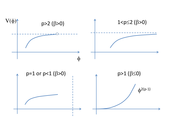
Figure 1: The schematic shape of $V(\phi)$ for several cases of $p$. $\beta=1/V(N\rightarrow\infty)$.

We also give the predictions for the tensor-to-scalar ratio $r$ and the running of the spectral index from Eq. (11) and Eq. (12):

$$r = \left\{\begin{array}[]{ll}\frac{8(p-1)}{N+\gamma^{2}(p-1)N^{p}}&\mbox{($\beta>0$)}\\ \frac{8(p-1)}{N}&\mbox{($\beta\leq 0$)}\\ \frac{8}{\gamma^{2}N}&\mbox{($p=1$)}\end{array}\right.$$ (47)

$$\frac{dn_{s}}{d\ln k} = -\frac{p}{N^{2}}\,.$$ (48)

$r$ varies from $8(p-1)/N$ (chaotic inflation model) to $8/\gamma^{2}N^{p}$ (modified T-model).

V Reheating Temperature

Once $V(N)$ is given, it is possible to connect $N$ and the reheating temperature $T_{\rm RH}$ assuming that $V(N)$ is valid for smaller $N$ mark1 ; kuro ; mark2 ; cook . For simplicity we consider the case of $n_{s}-1=-2/N$.

For the mode with wavenumber $k$, the comoving Hubble scale when this mode exited the horizon ($k=aH$) is related to that of the present time, $a_{0}H_{0}$ by

$$\frac{k}{a_{0}H_{0}}=\frac{H}{H_{0}}\frac{a}{a_{\rm end}}\frac{a_{\rm end}}{a_{\rm RH}}\frac{a_{\rm RH}}{a_{0}},$$ (49)

where $a_{\rm end}=a(t_{\rm end})$ and $a_{\rm RH}$ is the scale factor at the end of reheating. Here, by definition, $a/a_{\rm end}=e^{-N}$. Moreover, assuming that during the reheating phase the effective equation of state of the universe is matter-like due to coherent oscillation of the inflaton, the energy density at the end of inflation $\rho_{\rm end}$ is related to the energy density at the end of reheating $\rho_{\rm RH}$ by $\rho_{\rm RH}/\rho_{\rm end}=(a_{\rm end}/a_{\rm RH})^{3}$. $\rho_{\rm RH}$ is $\rho_{\rm RH}=(\pi^{2}g_{\rm RH}/30)T_{\rm RH}^{4}$, where $g_{\rm RH}$ is the effective number of relativistic degrees of freedom at the end of reheating. Further, assuming the conservation of entropy, $g_{S,\rm RH}a_{\rm RH}^{3}T_{\rm RH}^{3}=(43/11)a_{0}^{3}T_{0}^{3}$, where $g_{S,\rm RH}$ is the effective number of relativistic degrees of freedom for entropy at the end of reheating. Finally, the Hubble parameter during inflation is related to the scalar amplitude $A_{s}$ by $H^{2}=V/3=(\pi^{2}/2)rA_{s}$, where $A_{s}\simeq 2.14\times 10^{-9}$ from Planck Planck:2015 . Plugging these relations into Eq. (49), we obtain kuro

$$N=56.9-\ln\frac{k}{a_{0}H_{0}}-\ln\frac{h}{0.67}-\frac{1}{3}\ln\frac{\rho_{\rm end}}{\rho(N)}+\frac{1}{3}\ln\frac{T_{\rm RH}}{10^{9}{\rm GeV}}+\frac{1}{6}\ln r(N),$$ (50)

where $h$ denotes the dimensionless Hubble parameter and we have set $g_{\rm RH}=g_{S,\rm RH}$. From the requirement that the energy density at the end of reheating should be smaller than the energy density at the end of inflation, we have an upper bound on the reheating temperature $T_{\rm crit}$

$$\frac{\pi^{2}g_{\rm RH}}{30}T^{4}<\frac{\pi^{2}g_{\rm RH}}{30}T_{\rm crit}^{4}=\rho_{\rm end}=\frac{\rho_{\rm end}}{V}\frac{3\pi^{2}}{2}rA_{s}.$$ (51)

For the potential Eq. (16), the ratio is estimated as

$$\frac{\rho_{\rm end}}{\rho(N)}\simeq\frac{4}{3}\frac{V_{\rm end}}{V(N)}=\frac{4}{3}\left(\frac{\sqrt{1+2\gamma^{2}}-1}{\sqrt{1+2\gamma^{2}}+1}\right)\left(\frac{1+\gamma^{2}N}{\gamma^{2}N}\right),$$ (52)

where the factor $4/3$ comes from the contribution of the inflaton kinetic energy to $\rho_{\rm end}$ and we have defined the end of inflation by $\epsilon=V_{,N}/2V=1$. Therefore, $T_{\rm RH}$ can be written as

$$\frac{T_{\rm RH}}{10^{9}{\rm GeV}}=e^{3(N-56.9)}\left(\frac{k}{a_{0}H_{0}}\right)^{3}\frac{4}{3}\left(\frac{\sqrt{1+2\gamma^{2}}-1}{\sqrt{1+2\gamma^{2}}+1}\right)\left(\frac{1+\gamma^{2}N}{\gamma^{2}N}\right)\left(\frac{N+\gamma^{2}N^{2}}{8}\right)^{1/2},$$ (53)

where we have used Eq. (28) and assumed $h=0.67$. The upper bound of the reheating temperature Eq. (51) becomes

$$T_{\rm crit}=1.43\times 10^{16}{\rm GeV}\left(\frac{\sqrt{1+2\gamma^{2}}-1}{\sqrt{1+2\gamma^{2}}+1}\right)^{1/4}\left(\frac{1+\gamma^{2}N}{\gamma^{2}N}\right)^{1/4}\left(\frac{N+\gamma^{2}N^{2}}{8}\right)^{1/4},$$ (54)

where we have assumed $g_{\rm RH}=106.75$.

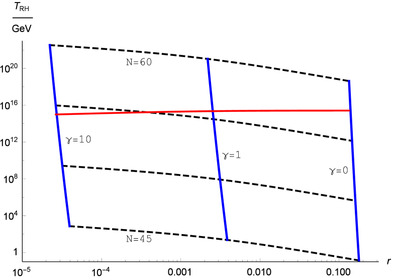
Figure 2: The reheating temperature versus $r$ for the model $n_{s}-1=-2/N$ for several $\gamma$ and $N$. The pivot scale is $k=0.05{\rm Mpc}^{-1}$. Blue curves for $\gamma=10,1,0$ from left to right; dotted curves for $N=60,55,50,45$ from top to bottom. The red curve is the upper bound on the reheating temperature $T_{\rm crit}$.

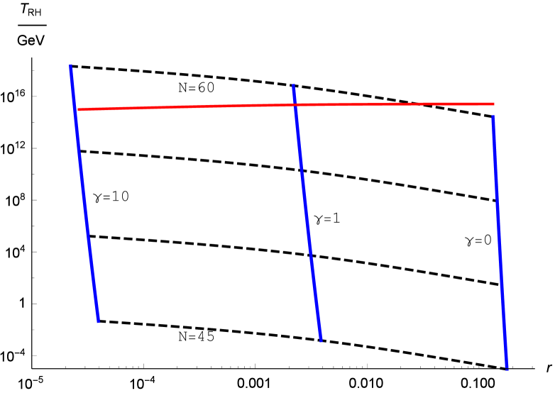
Figure 3: Same as Fig. 2 but for the pivot scale $k=0.002{\rm Mpc}^{-1}$.

In Fig. 2, we show the reheating temperature versus $r$ for several $\gamma$ and $N$ for the pivot scale $k=0.05{\rm Mpc}^{-1}$ at which Planck determines $n_{s}$ Planck:2015 . The blue curves are for $\gamma=10,1,0$ from left to right and dotted curves are for $N=60,55,50,45$ from top to bottom. For $n_{s}-1=-2/N$, the Planck result $n_{s}=0.9688\pm 0.0061$ Planck:2015 implies $53.8<N<79.7$. We find that for fixed $N$ $T_{\rm RH}$ slightly increases as $\gamma$ increases. This is because for larger $\gamma$ the slow-roll parameter $\epsilon$ becomes smaller and the Hubble parameter decreases less (in time) and hence the comoving Hubble horizon at the end of inflation $1/a_{\rm end}H_{\rm end}$ becomes smaller and this results in the shorter duration of the reheating phase.

The red curve is the upper bound on the reheating temperature $T_{\rm crit}$, Eq. (54). Since the dependence of $T_{\rm crit}$ on $N$ is very weak, we show the curve for $N=60$. The upper bound on the reheating temperature puts the upper bound on $N$: $N\lesssim 57$ for $\gamma=0$, $N\lesssim 56$ for $\gamma=1$ and $N\lesssim 54$ for $\gamma=10$. The result for $\gamma=0$ is consistent with mark2 . Combined with the measurement of $n_{s}$, $\gamma$ is constrained as $\gamma\lesssim 10$. Further combined with the constraint on $r<0.12$ by BICEP2/Planck bicep , we obtain $0.1\lesssim\gamma\lesssim 10$ and $10^{11}{\rm GeV}\lesssim T_{RH}\lesssim 2\times 10^{15}{\rm GeV}$. We note that the reheating temperature depends strongly on the equation of state during the reheating stage mark1 . The upper bounds on $N$ are significantly relaxed for the pivot scale $k=0.002{\rm Mpc}^{-1}$ because $T_{\rm RH}$ depends on $k^{3}$ (see Fig. 3).

VI Summary

Motivated by the relation $n_{s}-1\simeq-2/N$ indicated by recent cosmological observations, we derive the formulae to derive the inflaton potential $V(\phi)$ from $n_{s}(N)$. Applied to $n_{s}-1=-2/N$, to the first order in the slow-roll approximation, we find that the potential is classified into two categories depending on the value of $1/V(N\rightarrow\infty)$: T-model type ($\tanh^{2}(\gamma\phi/2)$) for $1/V(N\rightarrow\infty)>0$ or quadratic type ($\phi^{2}$) for $1/V(N\rightarrow\infty)\leq 0$. $\gamma$ is the ratio of $1/V(N\rightarrow\infty)$ to $-N^{2}(1/V)_{,N}$. We have calculated the reheating temperature versus the tensor-scalar ratio diagram. We have found that for fixed $N$ the reheating temperature slightly increases as $\gamma$ increases. For the pivot scale $k=0.05{\rm Mpc}^{-1}$, the upper bound on the reheating temperature puts the upper bound on the e-folding number, $N<60$.

We extend the classification of the potential $V(\phi)$ for $n_{s}-1=-p/N$. The shape of the potential is classified into four categories: symmetry-breaking type ($p>2$ and $1/V(N\rightarrow\infty)>0$), Starobinsky type ($1<p\leq 2$ and $1/V(N\rightarrow\infty)>0$), square-root/logarithmic type ( $0<p<1$ and $1/V(N\rightarrow\infty)>0$ or $p=1$), and power-law type $\phi^{2(p-1)}$ for $1/V(N\rightarrow\infty)\leq 0$. We find that only $p>1$ is allowed for the potential bounded from above.

We find that although $r$ depends on the ratio of the integration constant $\gamma$, the running of the spectral index does not (by construction). Therefore, the measurement of $r$ can be used to discriminate the model and to narrow down the shape, while the measurement of the running is used as a consistency check of the assumed form of $n_{s}(N)$.

References

- (1) P. A. R. Ade et al. [Planck Collaboration], arXiv:1502.01589 [astro-ph.CO]; P. A. R. Ade et al. [Planck Collaboration], arXiv:1502.02114 [astro-ph.CO].
- (2) A. D. Linde, Phys. Lett. B 129, 177 (1983).
- (3) A. A. Starobinsky, Phys. Lett. B 91, 99 (1980).
- (4) D. S. Salopek, J. R. Bond and J. M. Bardeen, Phys. Rev. D 40, 1753 (1989); F. L. Bezrukov and M. Shaposhnikov, Phys. Lett. B 659, 703 (2008) [arXiv:0710.3755 [hep-th]].
- (5) R. Kallosh and A. Linde, JCAP 1307, 002 (2013) [arXiv:1306.5220 [hep-th]].
- (6) R. Kallosh and A. Linde, arXiv:1502.07733 [astro-ph.CO].
- (7) R. Kallosh and A. Linde, arXiv:1503.06785 [hep-th].
- (8) V. Mukhanov, Eur. Phys. J. C 73, 2486 (2013) [arXiv:1303.3925 [astro-ph.CO]].
- (9) D. Roest, JCAP 1401, no. 01, 007 (2014) [arXiv:1309.1285 [hep-th]].
- (10) J. Garcia-Bellido and D. Roest, Phys. Rev. D 89, no. 10, 103527 (2014) [arXiv:1402.2059 [astro-ph.CO]].
- (11) P. Creminelli, S. Dubovsky, D. L. Nacir, M. Simonovi, G. Trevisan, G. Villadoro and M. Zaldarriaga, arXiv:1412.0678 [astro-ph.CO].
- (12) K. Kohri, Y. Oyama, T. Sekiguchi and T. Takahashi, JCAP 1310, 065 (2013) [arXiv:1303.1688 [astro-ph.CO]].
- (13) L. Dai, M. Kamionkowski and J. Wang, Phys. Rev. Lett. 113, 041302 (2014) [arXiv:1404.6704 [astro-ph.CO]].
- (14) S. Kuroyanagi, S. Tsujikawa, T. Chiba and N. Sugiyama, Phys. Rev. D 90, no. 6, 063513 (2014) [arXiv:1406.1369 [astro-ph.CO]].
- (15) J. B. Munoz and M. Kamionkowski, Phys. Rev. D 91, no. 4, 043521 (2015) [arXiv:1412.0656 [astro-ph.CO]].
- (16) J. L. Cook, E. Dimastrogiovanni, D. A. Easson and L. M. Krauss, JCAP 1504, no. 04, 047 (2015) [arXiv:1502.04673 [astro-ph.CO]].
- (17) P. A. R. Ade et al. [BICEP2 and Planck Collaborations], Phys. Rev. Lett. 114, no. 10, 101301 (2015) [arXiv:1502.00612 [astro-ph.CO]].