A novel variational model for image registration using Gaussian curvature

Abstract

Image registration is one important task in many image processing applications. It aims to align two or more images so that useful information can be extracted through comparison, combination or superposition. This is achieved by constructing an optimal transformation which ensures that the template image becomes similar to a given reference image. Although many models exist, designing a model capable of modelling large and smooth deformation field continues to pose a challenge. This paper proposes a novel variational model for image registration using the Gaussian curvature as a regulariser. The model is motivated by the surface restoration work in geometric processing [Elsey and Esedoglu, Multiscale Model. Simul., (2009), pp. 1549-1573]. An effective numerical solver is provided for the model using an augmented Lagrangian method. Numerical experiments can show that the new model outperforms three competing models based on, respectively, a linear curvature [Fischer and Modersitzki, J. Math. Imaging Vis., (2003), pp. 81-85], the mean curvature [Chumchob, Chen and Brito, Multiscale Model. Simul., (2011), pp. 89-128] and the diffeomorphic demon model [Vercauteren at al., NeuroImage, (2009), pp. 61-72] in terms of robustness and accuracy.

Key words: Image registration, Non-parametric image registration, Regularisation, Gaussian curvature, surface mapping.

1 Introduction

Image registration along with image segmentation are two of the most important tasks in imaging sciences problems. Here we focus on image registration. Much research work has been done; for an extensive overview of registration techniques see [28, 18, 20]. The methods can be classified into parametric and non-parametric image registration based on the geometric transformation. For the first category, the transformation is governed by a finite set of image features or by expanding a transformation in terms of basis functions. The second category (which is our main concern in this paper) of non-parametric image registration methods is not restricted to a certain parametrisable set. The problem is modelled as a functional minimisation via the calculus of variations. Given two images, the reference $R$ and template $T$, the functional consists of a distance measure $\mathcal{D}(T,R,\bm{u})$ and a regularisation term $\mathcal{S}(\bm{u})$ where $\bm{u}=(u_{1}(\bm{x}),u_{2}(\bm{x}))$ is the sought displacement vector at pixel $\bm{x}\in\Omega\subset\mathbb{R}^{2}$. The term $\mathcal{S}(\bm{u})$ removes the ill-posedness of the minimisation problem. We use the squared $\text{L}^{2}$ norm of the distance measure to quantify the differences between $T$ and $R$ as follows

$$\mathcal{D}(T,R,\bm{u})=\frac{1}{2}\int_{\Omega}(T(\bm{x}+\bm{u}(\bm{x}))-R(\bm{x}))^{2}d\Omega.$$ (1)

The distance measure in equation (1) is the sum of the squared difference (SSD) which is commonly used and optimal for mono-modal image registration with Gaussian noise. For multi-modal image registration where $T,R$ cannot be compared directly, other distance measures must be used [8]. Generally, the regularisation terms are inspired by physical processes such as elasticity, diffusion and motion curvature. As such, elastic image registration was introduced in [1] which assumed that objects are deformed as a rubber band.

In previous works, higher order regularisation models [7, 3] were found to be the most robust while the diffeomorphic demon model [22] offers the most physical transform in terms of (nearly) bijective mapping. Diffusion and total variation regularisation models based on first order derivatives are less complicated to implement but are at a disadvantage compared to higher order regularisation models based on second order derivatives due to two reasons. First, the former methods penalise rigid displacement. They cannot properly deal with transformations with translation and rotation. Second, low order regularisation is less effective than high order one in producing smooth transformations which are important in several applications including medical imaging. The work of [5, 6, 7] proposed a high order regularisation model named as a linear curvature, which is an approximation of the surface (mean) curvature and the model is invariant to affine registration. This work was later refined in [11, 9, 10] where a related approximation to the sum of the squares of the principal curvatures was suggested and higher order boundary conditions were recommended. Without any approximation to the mean curvature, the works in [3, 2] developed useful numerical algorithms for models based on the nonlinear mean curvature regularisation and observed advantages over the linear curvature models for image registration; however the effect of mesh folding (bijective maps) was not considered. The diffeomorphic demon model [23] is widely used due to its property of bijective maps; however the bijection is not precisely imposed. Another useful idea of enforcing bijection, beyond the framework we consider, is via minimising the Beltrami coefficient which measures the distortion of the quasi-conformal map of registration transforms [12].

In this paper we propose a high order registration model based on Gaussian curvature and hope to achieve large and smooth deformation without mesh folding. Although the Gaussian curvature is closely related to the mean curvature, it turns out our new model based on the Gaussian curvature is much better. The motivation of the proposed model comes from two factors. Firstly, we are inspired by the work of Elsey and Esedoglu [4] in geometry processing where Gaussian curvature of the image surface is used in a variational formulation. The authors proposed the Gaussian curvature as a natural analogue of the total variation of Rudin, Osher and Fatemi (ROF) [19] model in geometry processing. Aiming to generalise the ROF model to surface fairing where the convex shapes in 3D have similar interpretation to the monotone functions in 1D problems for the ROF model, they showed that, based on the Gauss Bonnet theorem, the complete analogy of the total variation regularisation for surface fairing is the energy functional of the Gaussian curvature. A very important fact pointed out in [4] stated that the mean curvature of the surface is not a suitable choice for surface fairing because the model is not effective for preserving important features such as creases and corners on the surface (although the model is still effective for removing noise). Their claims are also supported by the work of [13] where the authors illustrated several advantages of Gaussian curvature over mean curvature and total variation in removing noise in 2D images. First, Gaussian curvature preserves important structures such as edges and corners. Second, only Gaussian curvature can preserve structures with low gradient. Third, the model is effective in removing noise on small scale features. Thus, we believe that Gaussian curvature is a more natural physical quantity of the surface than mean curvature. Here we investigate the potential of using Gaussian curvature to construct a high order regularisation model for non-parametric image registration of mono-modal images.

The outline of this paper is as follows. In §2 we review the existing models for non-parametric image registration with focus on the demon, linear and mean curvature models. In §3 we introduce the mathematical background of Gaussian curvature for surfaces. In §4 we introduce a Gaussian curvature model and a numerical solver to solve the resulting Euler-Lagrange equations. We show in §5 some numerical tests including comparisons. Finally, we discuss the parameters’ selection issue for our model in §6 and present our conclusions in §7.

2 Review of Non-parametric Image Registration

In image registration, given two images $T$ and $R$ (which are assumed to be compactly supported and bounded operators $T,R:\Omega\subset\mathbb{R}^{d}\rightarrow\mathbb{R}^{+}$), the task is to transform $T$ to match $R$ as closely as possible. Although we consider $d=2$ throughout this paper, with some extra modifications, this work can be extended to $d=3$. In non-parametric image registration, the transformation is denoted by $\bm{\varphi}$ where $\bm{\varphi}$ is a vector valued function

$$\bm{\varphi}(\bm{x}):\mathbb{R}^{2}\rightarrow\mathbb{R}^{2}$$

where $\bm{x}=(x,y)$. To separate the overall mapping from the displacement field, we will define

$$\bm{\varphi}(\bm{x})=\bm{x}+\bm{u}(\bm{x})$$

where $\bm{u}(\bm{x})$ is the displacement field. Thus, finding $\bm{u}(\bm{x})$ is equivalent to finding $\bm{\varphi}$. A non-parametric image registration model takes the form

$$\min_{\bm{u}(\bm{x})}\mathcal{J}_{\gamma}(\bm{u}(\bm{x}))=\mathcal{D}(T,R,\bm{u}(\bm{x}))+\gamma\mathcal{S}(\bm{u}(\bm{x}))$$ (2)

where the distance measure $\mathcal{D}$ is given as in (1) and the choice of regulariser $\mathcal{S}(\bm{u}(\bm{x}))$ differentiates different models. Here $\bm{u}(\bm{x})$ is searched over a set $\mathcal{U}$ of admissible functions that minimise $\mathcal{J}_{\gamma}$ in (2). Usually, the set $\mathcal{U}$ is a linear subspace of a Hilbert space with Euclidean scalar product.

The force term $\bm{f}(\bm{u})$, to be used by all models, is the gradient of (1) with respect to the displacement field $\bm{u}(\bm{x})$

$$\bm{f}(\bm{u})=(f_{1}(\bm{u}),f_{2}(\bm{u}))^{T}=(T(\bm{x}+\bm{u}(\bm{x}))-R(\bm{x}))\nabla_{\bm{u}}T(\bm{x}+\bm{u}(\bm{x}))$$ (3)

which is non-linear. Different regularisation terms $\mathcal{S}(\bm{u}(\bm{x}))$ will lead to different non-parametric image registration models. Below we list three popular models selected for tests and comparisons.

Model LC. The first one is the linear curvature model by [6, 7, 15, 5], where

$${\mathcal{S}}^{\mbox{FMC}}(\bm{u})=\int_{\Omega}\Big{[}(\Delta u_{1})^{2}+(\Delta u_{2})^{2}\Big{]}d\Omega.$$ (4)

This term is an approximation of the surface curvature $\iota(u_{l})$ through the mapping $(x,y)\rightarrow(x,y,u_{l}(x,y)),\ l=1,2$ where

$$\iota(u_{l})=\nabla\cdot\frac{\nabla u_{l}}{\sqrt{|\nabla u_{l}|^{2}+1}}\ \approx\ \Delta u_{l}$$ (5)

when $|\nabla u_{l}|\approx 0$. The Euler Lagrange equation for (2) with ${\mathcal{S}}^{\mbox{FMC}}$ as the regularisation term is given by a fourth order PDE

$$\gamma\Delta^{2}\bm{u}+\bm{f}(\bm{u})=0$$ (6)

with boundary conditions $\Delta u_{l}=0,\nabla\Delta u_{l}\cdot\bm{n}=0,\ l=1,2$ and $\bm{n}$ the unit outward normal vector. The model consists of the second order derivative information of the displacement field which results in smoother deformations compared to those obtained using first order models based on elastic and diffusion energies. It is refined in [11, 9, 10] with nonlinear boundary conditions. The affine linear transformation belongs to the kernel ${\mathcal{S}}^{\mbox{FMC}}(\bm{u})$ which is not the case in elastic or diffusion registration.

Model MC. Next is the mean curvature model [3, 2]

$${\mathcal{S}}^{\mbox{MC}}(\bm{u})=\int_{\Omega}\Big{[}\Bbbk(\iota(u_{1}))+\Bbbk(\iota(u_{2}))\Big{]}d\Omega$$

where $\Bbbk(s)=\frac{1}{2}s^{2}$ and $\iota$ is as defined in (5). The Euler Lagrange equation for (2) with ${\mathcal{S}}^{\mbox{MC}}$ as the regularisation term is given by:

$$\gamma\nabla\cdot\Big{(}\frac{1}{\sqrt{|\nabla u_{l}|^{2}+1}}\nabla\Bbbk^{\prime}(\iota(u_{l}))-\frac{\nabla u_{l}\cdot\nabla\Bbbk^{\prime}(\iota(u_{l}))}{(\sqrt{|\nabla u_{l}|^{2}+1})^{3}}\nabla u_{l}\Big{)}+f_{l}(\bm{u})=0,\quad l=1,2$$ (7)

with boundary condition $\nabla u_{l}\cdot\bm{n}=\nabla\iota(u_{l})\cdot\bm{n}=0,\ l=1,2$. One can use the multigrid method to solve equation (7) as in [3]; refer also to [2] for multi-modality image registration work.

Model D. Finally Thirion [21] introduced the so-called demon registration method where every pixel in the image acts as the demons that force a pulling and pushing action in a similar way to what Maxwell did for solving the Gibbs paradox in thermodynamics. The original demon registration model is a special case of diffusion registration but it has been much studied and improved since 1998; see [17, 15, 25, 14]. The energy functional for the basic demon method is given by

$$\mathcal{S}(\bm{u})=\|R(\bm{x})-T(\bm{x}+\bm{\widetilde{u}}+\bm{u})\|^{2}+\frac{\sigma_{i}^{2}}{\sigma_{x}^{2}}\|\bm{u}\|^{2}$$ (8)

where $\bm{\widetilde{u}}$ is the current displacement field, $\sigma_{i}^{2}$ and $\sigma_{x}^{2}$ account for noise on the image intensity and the spatial uncertainty respectively. Equation (8) can be linearised using first order Taylor expansion,

$$\mathcal{J}(\bm{u})=\|R(\bm{x})-T(\bm{x}+\bm{\widetilde{u}})+J\bm{u}\|^{2}+\frac{\sigma_{i}^{2}}{\sigma_{x}^{2}}\|\bm{u}\|^{2}$$ (9)

where $J$ is given by

$$J=-\frac{\nabla R+\nabla T(\bm{x}+\bm{\widetilde{u}})}{2}$$

for an efficient second order minimisation. The first order condition of (9) leads to the new update for $\bm{\widetilde{u}}$

$$\bm{u}=-\frac{R(\bm{x})-T(\bm{x}+\bm{\widetilde{u}})}{\|J\|^{2}+\frac{\sigma_{i}^{2}}{\sigma_{x}^{2}}}J.$$

The additional use of $\bm{v}$ for $\bm{\varphi}=\exp(\bm{v})$ helps to achieve a nearly diffeormorphic transformation (mapping), where $\bm{v}$ is the stationary velocity field of the displacement field $\bm{u}$; see [24]. It should be remarked that the three main steps of the model cannot be combined into a single energy functional.

In a discrete setting, since the image domain $\Omega$ is a square, all variational models are discretised by finite differences on a uniform grid. Refer to [3, 15]. The vertex grid is defined by

$$\Omega^{h}=\big{\{}\bm{x}_{i,j}=(x_{i},y_{j})\ \ \big{|}\ \ 0\leq i\leq N_{1}-1,\ 0\leq j\leq N_{2}-1\big{\}}$$

where we shall re-use the notation $T$ and $R$ for discrete images of size $N_{1}\times N_{2}$.

3 Mathematical Background of the Gaussian curvature

In differential geometry, the Gaussian curvature problem seeks to identify a hypersurface of $\mathbb{R}^{d+1}$ as a graph $z=u(\bm{x})$ over $\bm{x}\in\Omega\subset\mathbb{R}^{d}$ so that, at each point of the surface, the Gaussian curvature is prescribed. Let $\kappa(\bm{x})$ denote the Gaussian curvature which is a real valued function in $\Omega\subset\mathbb{R}^{d}$. The problem is modelled by the following equation

$$\text{det}(D^{2}u)-\kappa(\bm{x})(1+|Du|^{2})^{(d+2)/2}=0$$ (10)

where $D$ is the first order derivative operator. Equation (10) is one of the Monge-Ampere equations. For $d=2$, we have

$$\kappa(\bm{x})\equiv-\kappa^{GC}=\frac{u_{xx}u_{yy}-u_{xy}u_{yx}}{(1+u_{x}^{2}+u_{y}^{2})^{2}}.$$ (11)

In [4], the authors define a regularisation term using the Gaussian curvature of a closed surface based on the Gauss-Bonnet theorem.

Theorem 3.1

Gauss-Bonnet Theorem. For a compact $C^{2}$ surface $\partial\Sigma$, we have

$$\int_{\partial\Sigma}\kappa^{GC}d\sigma=2\pi\chi$$

where $d\sigma$ is the length element to the surface and $\chi$ is the Euler characteristic of the surface.

Using this Theorem, it was shown in [4] that the complete analogy of the total variation regularisation for surface fairing is the energy functional of the Gaussian curvature. The analogous term $\mathcal{S}$, to the total variation of a function, that appears in the ROF model [19], is given by

$$\mathcal{S}=\int_{\partial\Sigma}|\kappa(\bm{x})|d\sigma$$

where $d\sigma$ is the length element to the surface $\partial\Sigma$.

Gaussian curvature is one of the fundamental second order geometric properties of a surface. According to the Gauss’s Theorema Egregium, Gaussian curvature is intrinsic. For a local isometric mapping $f:\partial\Sigma\rightarrow\partial\Sigma^{\prime}$ between two surfaces, Gaussian curvature remains invariant i.e. if $p\in\partial\Sigma$ and $p^{\prime}\in\partial\Sigma^{\prime}$, then $\kappa^{GC}(p)=\kappa^{GC}(p^{\prime})$ and the mapping $f$ is smooth and diffeomorphic.

We can also use a level set function to define the Gaussian curvature. Denote by $\phi$ the zero level set of the surface generated through the mapping $(x,y):\rightarrow(x,y,u(x,y))$. Then $\phi=u(x,y)-z$ and $\nabla\phi=(u_{x},u_{y},-1)^{T}$ where $u_{x}=\frac{\partial u}{\partial x}$ and $u_{y}=\frac{\partial u}{\partial y}$. The Gaussian curvature of the level set is given by

$$\kappa^{GC}=\frac{\nabla\phi H^{*}(\phi)\nabla\phi^{T}}{|\nabla\phi|^{4}}$$ (12)

where $\nabla\phi=(\phi_{x},\phi_{y},\phi_{z})^{T}$, $|\nabla\phi|=\sqrt{\phi_{x}^{2}+\phi_{y}^{2}+\phi_{z}^{2}}$, $H(\phi)$ is the Hessian matrix and $H^{*}(\phi)$ is the adjoint matrix for $H(\phi)$. We have

$$H(\phi)=\left[\begin{array}[]{ccc}u_{xx}&u_{xy}&0\\ u_{yx}&u_{yy}&0\\ 0&0&0\end{array}\right],\qquad H^{*}(\phi)=\left[\begin{array}[]{ccc}0&0&0\\ 0&0&0\\ 0&0&u_{xx}u_{yy}-u_{yx}u_{xy}\end{array}\right].$$

Then,

$$\kappa^{GC}=\frac{u_{yx}u_{xy}-u_{xx}u_{yy}}{(u_{x}^{2}+u_{y}^{2}+1)^{2}}.$$

This is why we set $\kappa^{GC}=-\kappa(\bm{x})$ in equation (11). We shall use $|\kappa^{GC}|$ to measure the Gaussian curvature as in [4] for a monotonically increasing function (since the functional should be nonnegative).

4 Image Registration based on Gaussian Curvature

Before introducing our new image registration model, we first illustrate some facts to support the use of Gaussian curvature.

4.1 Advantages of a Gaussian curvature

The total variation and Gaussian curvature. We use the volume based analysis introduced in [13] to compare two denoising models, respectively based on Gaussian curvature and the total variation:

$$\frac{\partial u}{\partial t}=\nabla\cdot\Big{(}\kappa\Big{(}\Big{|}\frac{u_{xy}^{2}-u_{xx}u_{yy}}{(u_{x}^{2}+u_{y}^{2}+1)^{2}}\Big{|}\Big{)}\nabla u\Big{)},$$ (13)

$$\frac{\partial u}{\partial t}=\nabla\cdot\frac{\nabla u}{|\nabla u|}.\hskip 71.13188pt$$ (14)

Consider, for each $\alpha>0$, the time change of the volume $v_{t,\alpha}=\{(x,y,z)\ |\ 0<z<|u(x,y,t)-\alpha|\}$ which is enclosed by the surface $z=u(x,y,t)$ and the plane $z=\alpha$. Assume $|u(x,y,t)-\alpha|=(u(x,y,t)-\alpha)s$ with $s$ either positive ($s=1$) or negative ($s=-1$) at all points. Denote by $c_{t,\alpha}$ the closed curve defined by the level set $u(x,y,t)=\alpha$ and accordingly by $d_{t,\alpha}$ the 2D region enclosed by $c_{t,\alpha}$. The volume change in $v_{t,\alpha}$ in time is given by

$$V=\frac{\partial}{\partial t}\int_{v_{t,\alpha}}dzdA=\frac{\partial}{\partial t}\int_{v_{t,\alpha}}\int_{0}^{|u(x,y,t)-\alpha|}dzdA=\frac{\partial}{\partial t}\int_{d_{t,\alpha}}|u(x,y,t)-\alpha|dA$$

where $dA$ is the area element. We now consider how $V$ changes from evolving (13) or (14).

If $u$ is the solution of equation (14), then from Gauss’ theorem

$$V =\frac{\partial}{\partial t}\int_{d_{t,\alpha}}|u(x,y,t)-\alpha|dA=s\int_{d_{t,\alpha}}\frac{\partial u}{\partial t}dA=s\int_{d_{t,\alpha}}\nabla\cdot\frac{\nabla u}{|\nabla u|}dA=s\int_{c_{t,\alpha}}\frac{\nabla u}{|\nabla u|}\cdot\bm{n}d\sigma$$

where $d\sigma$ is the length element and $\bm{n}$ is the unit normal vector to the curve $c_{t,\alpha}$ which is represented as $\bm{n}=s\frac{\nabla u}{|\nabla u|}$. Then

$$V=s^{2}\int_{c_{t,\alpha}}\frac{\nabla u}{|\nabla u|}\cdot\frac{\nabla u}{|\nabla u|}d\sigma=\int_{c_{t,\alpha}}d\sigma=|c_{t,\alpha}|$$

where $|c_{t,\alpha}|$ is the length of the curve $c_{t,\alpha}$. Furthermore, the volume variation in time is

$$\int_{d_{t+\delta t,\alpha}}|u(x,y,t+\delta t)-\alpha|dA \approx\int_{d_{t,\alpha}}|u-\alpha|dA+s\delta t\int_{d_{t,\alpha}}\frac{\partial u}{\partial t}dA=\int_{d_{t,\alpha}}\Big{[}|u-\alpha|+\delta t\frac{|c_{t,\alpha}|}{|d_{t,\alpha}|}\Big{]}dA$$

where $|d_{t,\alpha}|$ denotes the area of the region $d_{t,\alpha}$. We can see that the change in $u$ from $t$ to $t+\delta t$ is proportional to the ratio $\frac{|c_{t,\alpha}|}{|d_{t,\alpha}|}$. So, when this ratio is large (indicating possibly a noise presence), the total variation model reduces it and hence removes noise. However, important features of $u$ which have a large level set ratio are removed also and so not preserved by the total variation model (14).

Using similar calculations to before for the Gaussian curvature scheme (13), we have

$$V =\frac{\partial}{\partial t}\int_{d_{t,\alpha}}|u(x,y,t)-\alpha|dA=s\int_{d_{t,\alpha}}\nabla\cdot\Big{(}\kappa\Big{(}\Big{|}\frac{u_{xy}^{2}-u_{xx}u_{yy}}{(u_{x}^{2}+u_{y}^{2}+1)^{2}}\Big{|}\Big{)}\nabla u\Big{)}dA$$ (15)

$$=s\int_{c_{t,\alpha}}\Big{(}\kappa\Big{(}\Big{|}\frac{u_{xy}^{2}-u_{xx}u_{yy}}{(u_{x}^{2}+u_{y}^{2}+1)^{2}}\Big{|}\Big{)}\nabla u\Big{)}\cdot\bm{n}d\sigma\ =\int_{c_{t,\alpha}}\Big{(}\kappa\Big{(}\Big{|}\frac{u_{xy}^{2}-u_{xx}u_{yy}}{(u_{x}^{2}+u_{y}^{2}+1)^{2}}\Big{|}\Big{)}\Big{)}|\nabla u|d\sigma.$$

From here, we observe that the quantity $V$ for the subdomain $v_{t,\alpha}$ is dependent on the product of the variation and the Gaussian curvature on the level curve. The function $\kappa$ in (15) controls and scales the speed of the volume change in contrast to the total variation scheme where $V$ depends only on the variation of the level curve. Consider a point $p=(x_{0},y_{0},\alpha)$ where $\alpha=u(x_{0},y_{0})$. Gaussian curvature $\kappa=\kappa_{1}\kappa_{2}$ based on two principal curvatures $\kappa_{1}$ and $\kappa_{2}$ where $\kappa_{1}$ is the curvature of the level curve passing the point $p$ and $\kappa_{2}$ is the curvature of the path which passes the point and $\kappa_{2}$ is orthogonal to the level curve. If the Gaussian curvature on one level curve is zero then there is no change in $V$ regardless of variation on the level curves. In contrast, with the total variation, if there is a variation in the level curve, then there is a change in $V$. Based on this observation, we believe that the Gaussian curvature model is better than the total variation model for preserving features on surfaces.

The mean curvature and Gaussian curvature. The mean curvature (MC) $\iota=(\kappa_{1}+\kappa_{2})/2$ is also widely used. Next, we show that, though closely related, Gaussian curvature (GC) is better than mean curvature for surfaces in three ways.

First, Gaussian curvature is invariant under rigid and isometric transformations. In contrast, mean curvature is invariant under rigid transformations but not under isometric transformations. Rigid transformations preserve distance between two points while isometric transformations preserve length along surfaces and preserve angles between curves on surfaces. To illustrate invariance, consider a surface

$$z_{1}(x,y)=ax^{2}+by^{2},$$

whose Gaussian curvature and mean curvature are respectively

$$\kappa=\frac{0-(2a)(2b)}{(1+4a^{2}x^{2}+4b^{2}y^{2})^{2}},\qquad\iota=\frac{(1+4b^{2}y^{2})(2a)+(1+4a^{2}x^{2})(2b)}{(1+4a^{2}x^{2}+ab^{2}y^{2})^{3/2}}.$$

If we flip the surface upside down (isometric transformation) where $z_{1}^{\prime}(x,y)=-ax^{2}-by^{2}$, we will have the same value for the Gaussian curvature and a different value for the mean curvature. Thus, Gaussian curvature is invariant under isometric transformation.

Second, Gaussian curvature can be used to localise the tip of a surface better than mean curvature. Consider

$$z_{2}(x,y)=-\frac{1}{2}(x^{2}+y^{2}).$$

When we compute the mean and Gaussian curvature for the surface, we see that the value given by the Gaussian curvature is sharper than that of the mean curvature. The highest point of the Gaussian curvature is better distinguished from its neighbourhood compared to the highest point of the mean curvature.

Third, Gaussian curvature can locate saddle points better than mean curvature. Take

$$z_{3}(x,y)=-\frac{1}{2}(x^{2}-y^{2})$$

as one example. We can again compute its mean and Gaussian curvatures analytically. The mean curvature for this surface appears complex where the largest value is not at the saddle point and the saddle point cannot be easily located. However, Gaussian curvature gets its highest value at the saddle point and is therefore able to accurately identify the saddle point within its neighbourhood.

In addition to these three examples and observations, a very important fact pointed out in [4] states that the mean curvature of the surface is not a suitable choice for surface fairing because the model is not effective for preserving important features such as creases and corners on the surface (although the model is effective for removing noise). This is true when we refer to surface fairing (surface denoising) but not necessarily true for 2D image denoising. From the recent works done in image denoising [4, 13], we observe several advantages of Gaussian curvature over total variation and mean curvature. Therefore, we conjecture that Gaussian curvature may outperform existing models in image registration. To our knowledge there exists no previous work on this topic.

4.2 The proposed registration model

Now we return to the problem of how to align or register two image functions $T(\bm{x}),R(\bm{x})$. Let the desired and unknown displacement fields between $T$ and $R$ be the surface map $(x,y):\rightarrow(x,y,u_{l}(x,y))$ where $\ l=1,2$ and with $\bm{u}=(u_{1},u_{2})$. We propose our Gaussian curvature based image registration model as

$$\min_{\bm{u}\in C^{2}(\Omega)}\mathcal{J}_{\gamma}(\bm{u}(\bm{x}))=\frac{1}{2}\int_{\Omega}\left(T(\bm{x}+\bm{u})-R(\bm{x})\right)^{2}d\Omega+\gamma\mathcal{S}^{\text{GC}}(\bm{u}(\bm{x}))$$ (16)

where

$$\mathcal{S}^{\text{GC}}(\bm{u}(\bm{x}))=\sum_{l=1}^{2}{\mathcal{S}}^{GC}(u_{l}),\quad{\mathcal{S}}^{GC}(u_{l})=\int_{\Omega}\left|\frac{u_{l,xy}u_{l,yx}-u_{l,xx}u_{l,yy}}{(u_{l,x}^{2}+u_{l,y}^{2}+1)^{2}}\right|d\Omega.$$

The above model (16) leads to two Euler Lagrange equations:

$$\left\{\begin{aligned} &\gamma\nabla\cdot\left(\frac{4|u_{1,xy}u_{1,yx}-u_{1,xx}u_{1,yy}|}{\bm{\mathcal{N}}_{1}^{3}}\nabla u_{1}\right)+\gamma\nabla\cdot\bm{B}_{1,1}+\gamma\nabla\cdot\bm{B}_{1,2}+f_{1}=0\\ &\gamma\nabla\cdot\left(\frac{4|u_{2,xy}u_{2,yx}-u_{2,xx}u_{2,yy}|}{\bm{\mathcal{N}}_{2}^{3}}\nabla u_{2}\right)+\gamma\nabla\cdot\bm{B}_{2,1}+\gamma\nabla\cdot\bm{B}_{2,2}+f_{2}=0\\ \end{aligned}\right.$$ (17)

where

$$\bm{\mathcal{N}}_{l}=u_{l,x}^{2}+u_{l,y}^{2}+1,\ \ \bm{B}_{l,1}=\left(\left(-\frac{\mathcal{S}_{l}u_{l,yy}}{\bm{\mathcal{N}}_{l}}\right)_{x},\left(\frac{\mathcal{S}_{l}u_{l,xy}}{\bm{\mathcal{N}}_{l}}\right)_{x}\right)$$

$$\bm{B}_{l,2}=\left(\left(\frac{\mathcal{S}_{l}u_{l,yx}}{\bm{\mathcal{N}}_{l}}\right)_{y},\left(-\frac{\mathcal{S}_{l}u_{l,xx}}{\bm{\mathcal{N}}_{l}}\right)_{y}\right),\ \ \mathcal{S}_{l}=\text{sign}(u_{l,xy}u_{l,yx}-u_{l,xx}u_{l,yy})$$

$$\bm{f}=(f_{1},f_{2})^{T}=(T(\bm{x}+\bm{u})-R(\bm{x}))\nabla_{\bm{u}}T(\bm{x}+\bm{u}),\ l=1,2$$

and boundary conditions $\nabla u_{l}\cdot\bm{n}=0,\ l=1,2$, where $\bm{n}$ is the normal vector at the boundary $\partial\Omega$. Derivation of the resulting Euler-Lagrange equations for this model can be found in Appendix A. The equations are fourth order and nonlinear with anisotropic diffusion. Gradient descent type methods are not feasible and one way to solve them is by a geometric multigrid as in [3]. Here, instead, we present a fast and efficient way to solve the model (16) on a unilevel grid.

4.3 Augmented Lagrangian Method

The augmented Lagrangian method (ALM) is often used for solving constraint minimisation problems by replacing the original problem with an unconstrained problem. The method is similar to the penalty method where the constraints are incorporated in the objective functional and the problem is solved using alternating minimisation of each of the sub-problems. However, in ALM, there are additional terms in the objective functional known as Lagrange multiplier terms arising when incorporating the constraints. Similar works on the augmented Lagrangian method in image restoration can be found in [26, 27].

To proceed, we introduce two new dual variables $\bm{q}_{1}$ and $\bm{q}_{2}$ where $\bm{q}_{1}=\nabla u_{1}(\bm{x})$ and $\bm{q}_{2}=\nabla u_{2}(\bm{x})$. Consequently we obtain a system of second order PDEs which are more amendable to effective solution.

We obtain the following refined model for Gaussian curvature image registration

$$\min_{u_{1},u_{2},\bm{q}_{1},\bm{q}_{2}}\mathcal{J}(u_{1},u_{2},\bm{q}_{1},\bm{q}_{2}) =\mathcal{D}(T,R,\bm{u}(\bm{x}))+\gamma{\mathcal{S}}^{GC}(\bm{q}_{1})+\gamma{\mathcal{S}}^{GC}(\bm{q}_{2})$$

$$\text{s.t}\hskip 2.84544pt\bm{q}_{1}=\nabla u_{1}(\bm{x}),\bm{q}_{2}=\nabla u_{2}(\bm{x})$$

and further reformulate $\mathcal{J}(u_{1},u_{2},\bm{q}_{1},\bm{q}_{2})$ to get the augmented Lagrangian functional

$$\mathcal{L}^{GC}(u_{1},u_{2},\bm{q}_{1},\bm{q}_{2};\bm{\mu}_{1},\bm{\mu}_{2})= \frac{1}{2}\|T(\bm{x}+\bm{u}(\bm{x}))-R(\bm{x})\|^{2}_{2}+\gamma{\mathcal{S}}^{GC}(\bm{q}_{1})+\gamma{\mathcal{S}}^{GC}(\bm{q}_{2})$$ (18)

$$+\langle\bm{\mu}_{1},\bm{q}_{1}-\nabla u_{1}\rangle+\langle\bm{\mu}_{2},\bm{q}_{2}-\nabla u_{2}\rangle$$

$$+\frac{r}{2}\|\bm{q}_{1}-\nabla u_{1}\|^{2}_{2}+\frac{r}{2}\|\bm{q}_{2}-\nabla u_{2}\|^{2}_{2}$$

where $\bm{\mu}_{1},\bm{\mu}_{2}$ are the Lagrange multipliers, the inner products are defined via the usual integration in $\Omega$ and $r$ is a positive constant. We use an alternating minimisation procedure to find the optimal values of $u_{1},u_{2},\bm{q}_{1},\bm{q}_{2}$ and $\bm{\mu}_{1},\bm{\mu}_{2}$ where the process involves only two main steps.

Step 1. For the first step we need to update $\bm{q}_{1},\bm{q}_{2}$ for any given $u_{1},u_{2},\bm{\mu}_{1},\bm{\mu}_{2}$. The objective functional is given by

$$\min_{\bm{q}_{1},\bm{q}_{2}} \gamma{\mathcal{S}}^{GC}(\bm{q}_{1})+\gamma{\mathcal{S}}^{GC}(\bm{q}_{2})+\langle\bm{\mu}_{1},\bm{q}_{1}\rangle+\langle\bm{\mu}_{2},\bm{q}_{2}\rangle+\frac{r}{2}\|\bm{q}_{1}-\nabla u_{1}\|^{2}+\frac{r}{2}\|\bm{q}_{2}-\nabla u_{2}\|^{2}.$$

This sub-problem can be solved using the following Euler Lagrange equations:

$$\left\{\begin{aligned} &-\gamma\Big{(}\Big{(}\frac{(-q_{1,1})_{y}}{\Gamma_{1}^{2}}\Big{)}_{x}+\Big{(}\frac{-(q_{1,1})_{x}}{\Gamma_{1}^{2}}\Big{)}_{y}\Big{)}-\gamma\frac{4S_{1}D_{1}q_{1,2}}{\Gamma_{1}^{3}}+\mu_{1,2}+r(q_{1,2}-(u_{1})_{y})=0,\\ &-\gamma\Big{(}\Big{(}\frac{(q_{1,2})_{y}}{\Gamma_{1}^{2}}\Big{)}_{x}+\Big{(}\frac{-(q_{1,2})_{x}}{\Gamma_{1}^{2}}\Big{)}_{y}\Big{)}-\gamma\frac{4S_{1}D_{1}q_{1,1}}{\Gamma_{1}^{3}}+\mu_{1,1}+r(q_{1,1}-(u_{1})_{x})=0\end{aligned}\right.$$ (19)

where $D_{1}=\text{det}(\nabla\bm{q}_{1})=(q_{1,1})_{x}(q_{1,2})_{y}-(q_{1,1})_{y}(q_{1,2})_{x}$, $\Gamma_{1}=1+u_{1,x}^{2}+u_{1,y}^{2}$ and $S_{1}=\text{sign}\Big{(}\frac{D_{1}}{(\|\nabla u_{1}\|^{2}+1)^{2}}\Big{)}$. We have a closed form solution for this step, if solving alternatingly, where

$$q_{1,1} =\frac{\Gamma_{1}^{3}\Big{(}-\gamma\Big{(}\Big{(}\frac{(q_{1,2})_{y}}{\Gamma_{1}^{2}}\Big{)}_{x}+\Big{(}\frac{-(q_{1,2})_{x}}{\Gamma_{1}^{2}}\Big{)}_{y}\Big{)}+\mu_{1,1}-r(u_{1})_{x}\Big{)}}{-r\Gamma_{1}^{3}+\gamma 4S_{1}D_{1}},$$

$$q_{1,2} =\frac{\Gamma_{1}^{3}\Big{(}-\gamma\Big{(}\Big{(}\frac{(q_{1,1})_{y}}{\Gamma_{1}^{2}}\Big{)}_{x}+\Big{(}\frac{-(q_{1,1})_{x}}{\Gamma_{1}^{2}}\Big{)}_{y}\Big{)}+\mu_{1,2}-r(u_{1})_{y}\Big{)}}{-r\Gamma_{1}^{3}+\gamma 4S_{1}D_{1}}.$$

Similarly, we solve $q_{2,1},q_{2,2}$ from

$$\left\{\begin{aligned} &-\gamma\Big{(}\Big{(}\frac{(-q_{2,1})_{y}}{\Gamma_{2}^{2}}\Big{)}_{x}+\Big{(}\frac{-(q_{2,1})_{x}}{\Gamma_{2}^{2}}\Big{)}_{y}\Big{)}-\gamma\frac{4S_{2}D_{2}q_{2,2}}{\Gamma_{2}^{3}}+\mu_{2,1}+r(q_{2,2}-(u_{2})_{y})=0,\\ &-\gamma\Big{(}\Big{(}\frac{(q_{2,2})_{y}}{\Gamma_{2}^{2}}\Big{)}_{x}+\Big{(}\frac{-(q_{2,2})_{x}}{\Gamma_{2}^{2}}\Big{)}_{y}\Big{)}-\gamma\frac{4S_{2}D_{2}q_{2,1}}{\Gamma_{2}^{3}}+\mu_{2,1}+r(q_{2,1}-(u_{2})_{x})=0\\ \end{aligned}\right.$$ (20)

where $D_{2}=\text{det}(\nabla\bm{q}_{2})=(q_{2,1})_{x}(q_{2,2})_{y}-(q_{2,1})_{y}(q_{2,2})_{x}$, $\Gamma_{2}=1+u_{2,x}^{2}+u_{2,y}^{2}$ and $S_{2}=\text{sign}\Big{(}\frac{D_{2}}{(\|\nabla u_{2}\|^{2}+1)^{2}}\Big{)}$.

Step 2. For the second step we need to update $u_{1},u_{2}$ for any given $\bm{q}_{1},\bm{q}_{2}$ and $\bm{\mu}_{1},\bm{\mu}_{2}$ with the following functional

$$\min_{u_{1},u_{2}}\frac{1}{2}\|T(\bm{x}+\bm{u})-R(\bm{x})\|_{2}^{2}-\langle\bm{\mu}_{1},\nabla u_{1}\rangle-\langle\bm{\mu}_{2},\nabla u_{2}\rangle+\frac{r}{2}\|\bm{q}_{1}-\nabla u_{1}\|^{2}+\frac{r}{2}\|\bm{q}_{2}-\nabla u_{2}\|^{2}.$$

Thus, we have the following Euler Lagrange equations:

$$\left\{\begin{aligned} &-r\Delta u_{1}+f_{1}+\nabla\cdot\bm{\mu}_{1}+r\nabla\cdot\bm{q}_{1}=0\\ &-r\Delta u_{2}+f_{2}+\nabla\cdot\bm{\mu}_{2}+r\nabla\cdot\bm{q}_{2}=0\\ \end{aligned}\right.$$ (21)

with Neumann boundary conditions $\nabla u_{l}\cdot\bm{n}=0,l=1,2$. To solve equation (21), first, we linearise the force term $\bm{f}$ using Taylor expansion

$$f_{l}(u_{1}^{(k+1)},u_{2}^{(k+1)}) =f_{l}(u_{1}^{(k)},u_{2}^{(k)})+\partial_{u_{1}}f_{l}(u_{1}^{(k)},u_{2}^{(k)})\delta u_{l}^{(k)}+\partial_{u_{2}}f_{1}(u_{1}^{(k)},u_{2}^{(k)})\delta u_{2}^{(k)}+\ldots$$

$$\approx f_{l}(u_{1}^{(k)},u_{2}^{(k)})+\sigma^{(k)}_{l,1}\delta u_{1}^{(k)}+\sigma_{l,2}\delta u_{2}^{(k)}$$

where

$$\sigma^{(k)}_{l,1} =\partial_{u_{1}}f_{l}(u_{1}^{(k)},u_{2}^{(k)}),\sigma_{l,2}=\partial_{u_{2}}f_{l}(u_{1}^{(k)},u_{2}^{(k)}),\delta u_{1}^{(k)}=u_{1}^{(k+1)}-u_{1}^{(k)},\delta u_{2}^{(k)}=u_{2}^{(k+1)}-u_{2}^{(k)}.$$

Second, we approximate $\sigma^{(k)}_{l,1}$ and $\sigma^{(k)}_{l,2}$ with

$$\sigma^{(k)}_{l,1} =\Big{(}\partial u_{l}T(\bm{x}+\bm{u}^{(k)})\Big{)}\Big{(}\partial u_{1}T(\bm{x}+\bm{u}^{(k)})\Big{)}$$

$$\sigma^{(k)}_{l,2} =\Big{(}\partial u_{l}T(\bm{x}+\bm{u}^{(k)})\Big{)}\Big{(}\partial u_{2}T(\bm{x}+\bm{u}^{(k)})\Big{)}.$$

The discrete version of equation (21) is as follows

$$\bm{N}^{h}(\bm{u}^{h,(k)})\bm{u}^{h,(k+1)}=\bm{B}^{h}(\bm{u}^{h,(k)})$$ (22)

where

$$\bm{N}^{h}(\bm{u}^{(k)}) =\Big{[}\begin{array}[]{cc}-r\mathcal{L}+\sigma_{11}^{h}(\bm{u}^{h,(k)})&\sigma_{12}^{h}(\bm{u}^{h,(k)})\\ \sigma_{21}^{h}(\bm{u}^{h,(k)})&-r\mathcal{L}+\sigma_{22}^{h}(\bm{u}^{h,(k)})\\ \end{array}\Big{]},$$

$$\bm{B}^{h}(\bm{u}^{(k)}) =\Big{[}\begin{array}[]{c}-G^{h}_{1}+f^{h}_{1}(u_{1}^{(k)},u_{2}^{(k)})+\sigma_{11}^{h}(\bm{u}^{(k)})u_{1}^{h,(k)}+\sigma_{12}^{h}(\bm{u}^{h,(k)})u_{2}^{h,(k)}\\ -G^{h}_{2}+f^{h}_{2}(u_{1}^{(k)},u_{2}^{(k)})+\sigma_{21}^{h}(\bm{u}^{(k)})u_{1}^{h,(k)}+\sigma_{22}^{h}(\bm{u}^{h,(k)})u_{2}^{h,(k)}\\ \end{array}\Big{]},$$

$\mathcal{L}$ is the discrete version of the Laplace operator $\Delta$ and $G^{h}_{l}$ is the discrete version of

$$\nabla\cdot\bm{\mu}_{l}+r\nabla\cdot\bm{q}_{l},\ l=1,2.$$

Third, we solve the system of equation (22) using a weighted pointwise Gauss Siedel method

$$\bm{u}^{h,(k+1)}=(1-\omega)\bm{u}^{h,(k)}+\omega\Big{(}\bm{N}^{h}(\bm{u}^{(k)})\Big{)}^{-1}\bm{B}^{h}(\bm{u}^{(k)})$$

where $\omega\in(0,2)$ and we choose $\omega=0.9725$.

The iterative algorithm to solve (18) is now summarised as follows.

Algorithm 1 Augmented Lagrangian method for the Gaussian Curvature Image Registration.

1. Initialise $\bm{\mu}_{1}=\bm{\mu}_{2}=\bm{0},\bm{u}(\bm{x})=0,\gamma,r$.

2. For $k=0,1,...,IMAX$

   1. Step 1: Solve (19-20) for $(\bm{q}_{1}^{(k+1)},\bm{q}_{2}^{(k+1)})$ with $(u_{1},u_{2})=(u_{1}^{(k)},u_{2}^{(k)})$.

   2. Step 2: Solve (21) for $(u_{1}^{(k+1)},u_{2}^{(k+1)})$ with $(\bm{q}_{1},\bm{q}_{2})=(\bm{q}_{1}^{(k+1)},\bm{q}_{2}^{(k+1)})$.

   3. Step 3: Update Lagrange multipliers.
      $\bm{\mu}_{1}^{(k+1)}=\bm{\mu}_{1}^{(k)}+r(\bm{q}_{1}^{(k+1)}-\nabla u_{1}^{(k+1)})$, $\bm{\mu}_{2}^{(k+1)}=\bm{\mu}_{2}^{(k)}+r(\bm{q}_{2}^{(k+1)}-\nabla u_{2}^{(k+1)})$

3. End for.

5 Numerical Results

We use two numerical experiments to examine the efficiency and robustness of the Algorithm 1 on a variety of deformations. To judge the quality of the alignment we calculate the relative reduction of the similarity measure

$$\varepsilon=\frac{\mathcal{D}(T,R,\bm{u})}{\mathcal{D}(T,R)}$$

and the minimum value of the determinant of the Jacobian matrix $J$ of the transformation, denoted as ${\cal F}$

$$J =\left[\begin{array}[]{cc}1+u_{1,x}&u_{1,y}\\ u_{2,x}&1+u_{2,y}\end{array}\right],\hskip 2.84544pt{\cal F}=\text{min}\left(\det(J)\right).$$ (23)

We can observe that when ${\cal F}>0$, the deformed grid is free from folding and cracking.

All experiments were run on a single level. Experimentally, we found that $r\in[0.02,2]$ works well for several types of images. As for the stopping criterion, we use $tol=0.001$ for the residual of the Euler-Lagrange equations (19)-(21) and the maximum number of iterations is 30. Experiments were carried out using Matlab R2014b with Intel(R) core (TM) i7-2600 processor and 16G RAM.

5.1 Test 1: A Pair of Smooth X-ray Images

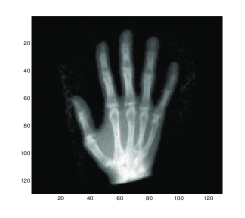
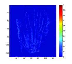
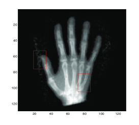
Images for Test 1 are taken from [16] where X-ray images of two hands of different individuals need to be aligned. The size of images are $128\times 128$ and the recovered transformation is expected to be smooth. The scaled version of the transformation and the transformed template image is given in Figures 1 (d) and (e) respectively. The transformation is smooth and the model is able to solve such a problem.

(a) $T$

(b) $R$

(c) $T-R$

(d) $\bm{x}+\bm{u}(\bm{x})$

(e) $T(\bm{x}+\bm{u}(\bm{x}))$

(f) $T(\bm{x}+\bm{u}(\bm{x}))-R$

Figure 1: Test 1 (X-ray hand). Illustration of the effectiveness of Gaussian curvature with smooth problems. On the top row, from left to right: (a) template, (b) reference and (c) the difference before registration. On the bottom row, from left to right: (d) the transformation applied to a regular grid, (e) the transformed template image and (f) the difference after registration. As can be seen from the result (e) and the small difference after registration (f), Gaussian curvature is able to solve smooth problems.

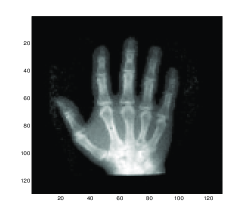
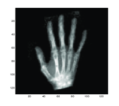
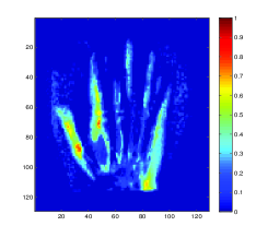
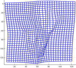
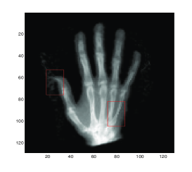
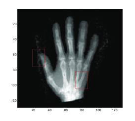
For comparison, the transformed template images for the diffeormorphic demon method, linear, mean and Gaussian curvatures are shown in Figures 2 (a), (b), (c) and (d) respectively. We can observe that there are some differences of these images inside the red boxes where only Gaussian curvature delivering the best result of the features inside the boxes.

(a) Model D

(b) Model LC

(c) Model MC

(d) Gaussian curvature

Figure 2: Test 1 (X-ray hand). Comparison of Gaussian curvature with competing methods. The transformed template image using (a) Model D, (b) Model LC, (c) Model MC and (d) Gaussian curvature. Note the difference of these three images inside the red boxes.

Measure	Model D		Model LC		Model MC	GC
	ML	SL	ML	SL	SL	SL
$\gamma$	1.6	1.6	0.1	0.5	0.0001	0.0001
Time (s)	15.19	186.48	84.33	12.98	275.3	953.15
$\varepsilon$	0.1389	0.1229	0.0720	0.3780	0.0964	0.0582
${\cal F}$	0.0600	0.1082	0.3894	0.1973	0.6390	0.3264

Table 1: Quantitative measurements for all models for Test 1. ML and SL stand for multi and single level respectively. $\gamma$ is chosen as small as possible such that ${\cal F}>0$ for all methods. ${\cal F}>0$ indicates the deformation consists of no folding and cracking of the deformed grid. We can see that the smallest value of $\varepsilon$ is given by Gaussian curvature (GC).

We summarised the results for Test 1 in Table 1 where ML and SL stand for multi and single level respectively. For all models, $\gamma$ is chosen as small as possible such that ${\cal F}>0$. We can see that the fastest model is the diffeormorphic demon, followed by linear and mean curvature. The current implementation for Gaussian curvature is on single level and the model uses augmented Lagrangian method which has four dual variables and four lagrange multipliers terms. Thus, it requires more computational time than the other models.

5.2 Test 2: A Pair of Brain MR Images

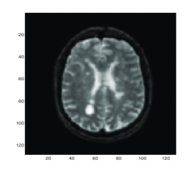
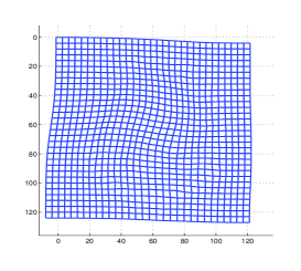
We take as Test 2 a pair of medical images of size $256\times 256$ from the Internet Brain Segmentation Repository (IBSR) http://www.cma.mgh.harvard.edu/ibsr where 20 normal MR brain images and their manual segmentations are provided. We choose the particular pair of individuals with different sizes of ventricle to illustrate a large deformation problem. Figure 3 shows the test images and the registration results using Gaussian curvature model. We can see that the model is able to solve real medical problems involving large deformations, which is particularly important for atlas construction in medical applications.

(a) $T$

(b) $R$

(c) $T-R$

(d) $\bm{x}+\bm{u}(\bm{x})$

(e) $T(\bm{x}+\bm{u}(\bm{x}))$

(f) $T(\bm{x}+\bm{u}(\bm{x}))-R$

Figure 3: Test 2: A pair of Brain MR images. Illustration of the effectiveness of Gaussian curvature with real medical images. On the top row, from left to right: (a) template, (b) reference and (c) the difference before registration. On the bottom row, from left to right: (d) the transformation applied to a regular grid, (e) the transformed template image and (f) the difference after registration. As can be seen from the result (e) and the small difference after registration (f), Gaussian curvature can be applied to real medical images and is able to obtain good results.

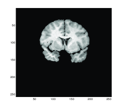
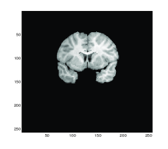
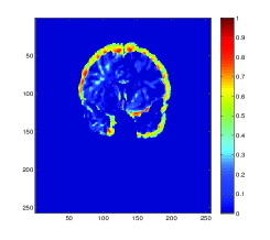
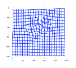
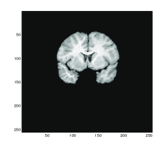
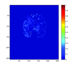
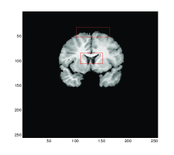
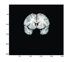
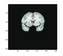
Figure 4 shows the transformed template images for all four methods. We can see that Gaussian curvature gives the best result inside the red boxes in comparison with the diffeomorphic demon, the linear and mean curvature models as depicted in Figure 4 (d).

(a) Model D

(b) Model LC

(c) Model MC

(d) Gaussian curvature

Figure 4: Test 2: A pair of Brain MR images. Comparison of Gaussian curvature with competing methods. The transformed template image using (a) Model D, (b) Model LC, (c) Model MC, and (d) Gaussian curvature. Notice the differences of these three images inside the red boxes. Considerably more accurate results are obtained, particularly within these significant regions, by employment of the Gaussian curvature model.

Measure	Model D		Model LC		Model MC	GC
	ML	SL	ML	SL	SL	SL
$\gamma$	1.2	1.4	0.16	2.0	0.0001	0.0001
Time (s)	23.89	209.00	275.04	35.70	830.22	1053.7
$\varepsilon$	0.2004	0.7580	0.1128	0.4283	0.1998	0.1062
${\cal F}$	0.0277	0.0387	0.3157	0.0148	0.8240	0.0138

Table 2: Quantitative measurements for all models for Test 2. ML and SL stand for multi and single level respectively. $\gamma$ is chosen to be as small as possible such that ${\cal F}>0$ for all models. ${\cal F}>0$ indicates the deformation consists of no folding and cracking of the deformed grid. We can see that the smallest value of $\varepsilon$ is given by Gaussian curvature (GC).

The values of the quantitative measurements for Test 2 are recorded in Table 2 where the lowest values of $\varepsilon$ are given by the Gaussian curvature model indicating higher similarity between the transformed template result and the reference image. However, our proposed model required more time than the other models since the model consists more variables than the others.

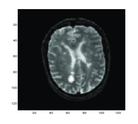
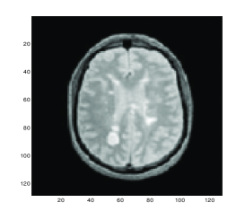
A brief summary. The linear curvature model is relatively easy to solve, based on approximation of the mean curvature. The mean curvature model for image registration is highly nonlinear, making it challenging to solve. The Gaussian curvature resembles the mean curvature in many ways, though different, but its model appears to deliver better quality than the mean curvature. The diffeormorphic demon model is equivalent to the second order gradient descent on the SSD as shown in [17]. The model is only limited to mono-modality images and it is not yet applicable to multi-modality images. Our Gaussian curvature model however can be easily modified to work with multi-modality images by replacing the SSD by a mutual information or normalised gradient fields based regularizer; an optimal solver is yet to be developed. We show one example of extension to a pair of multi-modality images in Fig.5.

(a) $T$

(b) $R$

(c) $T(\bm{x}+\bm{u}(\bm{x}))$

(d) $\bm{x}+\bm{u}(\bm{x})$

Figure 5: Results of Gaussian curvature image registration for multi-modality images. The model is able to register multi-modality images with mutual information as the distance measure.

6 Conclusions

We have introduced a novel regularisation term for non-parametric image registration based on the Gaussian curvature of the surface induced by the displacement field. The model can be effectively solved using the augmented Lagrangian and alternating minimisation methods. For comparison, we used three models: the linear curvature [6], the mean curvature [3] and the demon algorithm [24] for mono-modality images. Numerical experiments show that the proposed model delivers better results than the competing models.

Appendix A – Derivation of the Euler-Lagrange Equations

Let $q_{1}=u_{x}$ and $q_{2}=u_{y}$; then we can write the Gaussian curvature regularisation term as

$${\mathcal{S}}^{GC}(q_{1},q_{2})=\int_{\Omega}\Big{|}\frac{q_{1,x}q_{2,y}-q_{1,y}q_{2,x}}{(1+q_{1}^{2}+q_{2}^{2})^{2}}\Big{|}dxdy.$$

From the optimality condition $\frac{d{\mathcal{S}}^{GC}(q_{1},q_{2})}{dq_{1}}=\frac{d{\mathcal{S}}^{GC}(q_{1},q_{2})}{dq_{2}}=0$, then $\frac{d}{d\epsilon_{1}}{\mathcal{S}}^{GC}(q_{1}+\epsilon_{1}\varphi_{1},q_{2})\Big{|}_{\epsilon_{1}=0}=0$ and $\frac{d}{d\epsilon_{2}}{\mathcal{S}}^{GC}(q_{1},q_{2}+\epsilon_{2}\varphi_{2})\Big{|}_{\epsilon_{2}=0}=0$. In details,

$$\mbox{ }\begin{aligned} \frac{d}{d\epsilon_{1}}\int_{\Omega}\Big{|}\frac{(q_{1}+\epsilon_{1}\varphi_{1})_{x}q_{2,y}-(q_{1}+\epsilon_{1}\varphi_{1})_{y}q_{2,x}}{(1+(q_{1}+\epsilon_{1}\varphi_{1})^{2}+q_{2}^{2})^{2}}\Big{|}dxdy\Big{|}_{\epsilon=0}=\mbox{ }\hskip 71.13188pt&\\ \int_{\Omega}S\frac{d}{d\epsilon_{1}}\left[\frac{(q_{1}+\epsilon_{1}\varphi_{1})_{x}q_{2,y}-(q_{1}+\epsilon_{1}\varphi_{1})_{y}q_{2,x}}{(1+(q_{1}+\epsilon_{1}\varphi_{1})^{2}+q_{2}^{2})^{2}}\right]dxdy\Big{|}_{\epsilon=0}=0&\end{aligned}$$ (24)

where $S=\text{sign}\left(\frac{q_{1,x}q_{2,y}-q_{1,y}q_{2,x}}{(1+q_{1}^{2}+q_{2}^{2})^{2}}\right)$. From (24),

$$\int_{\Omega}S\left[\frac{\varphi_{1,x}q_{2,y}-\varphi_{1,y}q_{2,x}}{(1+q_{1}^{2}+q_{2}^{2})^{2}}+(q_{1,x}q_{2,y}-q_{1,y}q_{2,x})(-4\varphi_{1}q_{1}(1+q_{1}^{2}+q_{2}^{2})^{-3})\right]dxdy$$

$$=\int_{\Omega}\frac{S\varphi_{1,x}q_{2,y}}{\Gamma^{2}}-\frac{S\varphi_{1,y}q_{2,x}}{\Gamma^{2}}-\frac{4SDq_{1}\varphi_{1}}{\Gamma^{3}}dxdy=0,$$

$$\mbox{}\text{ where}\hskip 2.84544pt\Gamma=1+q_{1}^{2}+q_{2}^{2},D=q_{1,x}q_{2,y}-q_{1,y}q_{2,x}.$$

Using the Green theorem $\int_{\partial\Omega}\phi\bm{\omega}\cdot\bm{n}ds-\int_{\Omega}\phi\text{div}(\bm{\omega})dxdy=\int_{\Omega}\nabla\phi\cdot\bm{\omega}dxdy,$ we have,

$$\int_{\Omega}\frac{S\varphi_{1,x}q_{2,y}}{\Gamma^{2}}-\frac{S\varphi_{1,y}q_{2,x}}{\Gamma^{2}}dxdy=\int_{\partial\Omega}\varphi_{1}\left(\frac{Sq_{2,y}}{\Gamma^{2}},\frac{Sq_{2,x}}{\Gamma^{2}}\right)\cdot\bm{n}ds-\int_{\Omega}\varphi_{1}\text{div}\left(\frac{Sq_{2,y}}{\Gamma^{2}},\frac{Sq_{2,x}}{\Gamma^{2}}\right)=0$$

where $\phi=\varphi_{1},\bm{\omega}=\left(\frac{Sq_{2,y}}{\Gamma^{2}},\frac{Sq_{2,x}}{\Gamma^{2}}\right)$. Setting the boundary integral to zero, then we derive

$$\int_{\Omega}\varphi_{1}\text{div}\left(\frac{Sq_{2,y}}{\Gamma^{2}},\frac{Sq_{2,x}}{\Gamma^{2}}\right)=0.$$

Finally, we use the fundamental lemma of calculus of variation to get:

$$\nabla\cdot\left(\frac{Sq_{2,y}}{\Gamma^{2}},\frac{Sq_{2,x}}{\Gamma^{2}}\right)-\frac{4SDq_{1}}{\Gamma^{3}}=0.$$

Similarly, for $\frac{d}{d\epsilon_{2}}{\mathcal{S}}^{GC}(q_{1},q_{2}+\epsilon_{2}\varphi_{2})\Big{|}_{\epsilon_{2}=0}=0$, we finally obtain equation (17). $\Box$

Authors’ home page:      http:$\backslash\backslash$www.liv.ac.uk/cmit

References

- [1] C. Broit. Optimal registration of deformed images. PhD thesis, University of Pennsylvania, 1981.
- [2] N. Chumchob and K. Chen. Improved variational image registration model and a fast algorithm for its numerical approximation. Numer. Meth. PDE, 28(6):1966–1995, 2012.
- [3] N. Chumchob, K. Chen, and C. Brito-Loeza. A fourth-order variational image registration model and its fast multigrid algorithm. SIAM Multiscale Model. Simul., 9(1):89–128, 2011.
- [4] M. Elsey and S. Esedog¯lu. Analogue of the total variation denoising model in the context of geometry processing. SIAM Multiscale Model. Simul., 7(4):1549–1573, 2009.
- [5] B. Fischer and J. Modersitzki. Curvature based registration with applications to mr-mammography. In Proc. Int. Conf. Computational Science-Part III, 2002.
- [6] B. Fischer and J. Modersitzki. Curvature based image registration. J. Math. Imaging Vis., 18(1):81–85, 2003.
- [7] B. Fischer and J. Modersitzki. A unified approach to fast image registration and a new curvature based registration technique. Linear Algebra Appl., 380:107–124, 2004.
- [8] E. Haber and J. Modersitzki. Beyond mutual information: A simple and robust alternative. In Bildverarbeitung für die Medizin 2005, pages 350–354. Springer, 2005.
- [9] S. Henn. A full curvature based algorithm for image registration. J. Math. Imaging Vis., 24(2):195–208, 2006.
- [10] S. Henn. A translation and rotation invariant Gauss–newton like scheme for image registration. BIT, 46(2):325–344, 2006.
- [11] S. Henn and K. Witsch. A variational image registration approach based on curvature scale space. In Scale Space and PDE Methods in Computer Vision, pages 143–154. Springer Berlin Heidelberg, 2005.
- [12] K. C. Lam and L. M. Lui. Landmark- and intensity-based registration with large deformations via quasi-conformal maps. SIAM J. Imaging Sci., 7:2364–2392, 2014.
- [13] S.-H. Lee and J. K. Seo. Noise removal with Gauss curvature-driven diffusion. Trans. Img. Proc., 14(7):904–909, 2005.
- [14] H. Lombaert, L. Grady, X. Pennec, N. Ayache, and F. Cheriet. Spectral demons - image registration via global spectral correspondence. In Computer Vision – ECCV 2012, pages 30–34. Springer Berlin Heidelberg, 2012.
- [15] J. Modersitzki. Numerical Methods for Image Registration. Oxford University Press, 2004.
- [16] J. Modersitzki. Flexible Algorithms for Image Registration. SIAM publications, 2009.
- [17] X. Pennec, P. Cachier, and N. Ayache. Understanding the “demon’s algorithm”: 3D non-rigid registration by gradient descent. In Proc. MICCAI’99, pages 597–605. Springer, 1999.
- [18] J. P. Pluim, J. B. Maintz, and M. A. Viergever. Mutual information based registration of medical images: a survey. IEEE T. Med. Imaging, 22(8):986–1004, 2003.
- [19] L. I. Rudin, S. Osher, and E. Fatemi. Nonlinear total variation based noise removal algorithms. Physica D: Nonlinear Phenomena, 60(1-4):259–268, 1992.
- [20] A. Sotiras, C. Davatzikos, and N. Paragios. Deformable medical image registration: A survey. IEEE Trans. Med. Imaging, 32(7):1153–1190, 2013.
- [21] J. P. Thirion. Image matching as a diffusion process: an analogy with maxwell’s demons. Med. Image Anal., 2(3):243–260, 1998.
- [22] T. Vercauteren, X. Pennec, E. Malis, A. Perchant, and N. Ayache. Insight into efficient image registration techniques and the demons algorithm. In Information Processing in Medical Imaging, pages 495–506. Springer, 2007.
- [23] T. Vercauteren, X. Pennec, A. Perchant, and N. Ayache. Non-parametric diffeomorphic image registration with the demons algorithm. In Medical Image Computing and Computer-Assisted Intervention–MICCAI 2007, pages 319–326. Springer, 2007.
- [24] T. Vercauteren, X. Pennec, A. Perchant, and N. Ayache. Diffeomorphic demons: efficient non-parametric image registration. Neuroimage, 45(1):S61–S72, 2009.
- [25] H. Wang, L. Dong, J. O’Daniel, R. Mohan, A. S. Garden, K. K. Ang, D. A. Kuban, M. Bonnen, J. Y. Chang, and R. Cheung. Validation of an accelerated ’demons’ algorithm for deformable image registration in radiation therapy. Phys. Med. Biol., 50(12):2887–905, 2005.
- [26] W. Zhu and T. Chan. Image denoising using mean curvature of image surface. SIAM J. Imaging Sci., 5(1):1–32, 2012.
- [27] W. Zhu, X.-C. Tai, and T. Chan. A fast algorithm for a mean curvature based image denoising model using augmented lagrangian method. In Efficient Algorithms for Global Optimization Methods in Computer Vision, pages 104–118. Springer Berlin Heidelberg, 2014.
- [28] B. Zitová and J. Flusser. Image registration methods: a survey. Image Vision Comput., 21(11):977–1000, 2003.
Authors’ home page: http:www.liv.ac.uk/cmit