Shock waves in quasi one-dimensional Bose-Einstein condensate

Abstract

We study analytically and numerically the generation of shock waves in a quasi one-dimensional Bose-Einstein condensate (BEC) made of dilute and ultracold alkali-metal atoms. For the BEC we use an equation of state based on a 1D nonpolynomial Schrödinger equation (1D NPSE), which takes into account density modulations in the transverse direction and generalizes the familiar 1D Gross-Pitaevskii equation (1D GPE). Comparing 1D NPSE with 1D GPE we find quantitative differences in the dynamics of shock waves regarding the velocity of propagation, the time of formation of the shock, and the wavelength of after-shock dispersive ripples.

1 Introduction

In the past years the zero-temperature hydrodynamic equations of superfluids landau have been successfully applied to investigate dilute and ultracold bosonic superfluids, i.e. Bose-Einstein condensates (BECs) made of confined alkali-metal atoms bec-review . More recently it has been shown pitaevskii that also fermionic superfluids in the BCS-BEC crossover can be modelled by hydrodynamic equations and their generalizations luca12 .

The formation of shock waves induced by an ad hoc external perturbation has been observed in BECs hau ; cornell ; hoefer ; davis and in the unitary Fermi gas thomas . Motivated by these low temperature experiments on shock waves in atomic superfluids, some authors have theoretically analyzed the formation of shock waves in various configurations of bosonic zak ; damski ; gammal ; perez ; muga ; noi and fermionic superfluids noi2a ; noi2b ; bulgac . In particular, shock waves of a strictly one-dimensional (1D) superfluid in the regime of quasi condensation have been studied in Refs. zak ; damski by using the 1D Gross-Pitaevskii equation (1D GPE).

Here we extend their analysis by studying a cylindrically confined BEC, whose transverse width $\sigma$ is not frozen but depends on the longitudinal axial density $\rho$ npse ; gll , and adopting the 1D nonpolynomial Schrödinger equation (1D NPSE) npse . Indeed, 1D NPSE is a more realistic model for a comparison with experiments, where quasi one-dimensional BECs are produced by imposing a very strong harmonic confinement of characteristic length $a_{\bot}$ along two directions. In this paper we find that the shock waves obtained by using 1D GPE, based on the hypothesis of a strictly one-dimensional Bose-Einstein condensate, show quantitative differences with respect to the ones derived from 1D NPSE.

2 Hydrodynamic equations for a quasi 1D bosonic superfluid

We consider a dilute bosonic superfluid at zero temperature that is freely propagating in the longitudinal axial direction $z$ and is confined in the transverse directions $(x,y)$ by a harmonic potential of frequency $\omega_{\bot}$ and characteristic length $a_{\bot}=(\hbar/(m\omega_{\bot}))^{1/2}$ with $m$ the mass of a bosonic particle. Under the adiabatic hypothesis that the transverse profile of the superfluid has a Gaussian shape with a size depending on the longitudinal density npse ; gll , one finds the following dimensionless hydrodynamic equations for the axial dynamics of the superfluid

$${\partial\rho\over\partial t}+{\partial\over\partial z}\left(\rho v\right)=0\;,$$ (1)

$${\partial v\over\partial t}+{\partial\over\partial z}\left({v^{2}\over 2}+\mu(\rho)\right)=0\;,$$ (2)

where $\rho(z,t)$ is the superfluid axial density at time $t$, $v(z,t)$ is the superfluid axial velocity at time $t$ and $\mu(\rho)$ is the bulk chemical potential. Here length is in units of $a_{\bot}$, time in units of $\omega_{\bot}^{-1}$, energy in units of $\hbar\omega_{\bot}$, and axial density in units of $a_{\bot}^{-1}$. Thus the axial dynamics of the confined superfluid depends crucially on the functional form of the bulk chemical potential, that is given by gll

$$\mu={3\over 2}\ \rho^{2}\ L[{g\over\rho\sigma^{2}}]+{1\over\sigma^{2}}\;,$$ (3)

where

$$\sigma^{4}=1+g\ \rho\ L^{\prime}[{g\over\rho\sigma^{2}}]$$ (4)

is the transverse width, $g=2a_{s}/a_{\bot}$ is the interaction strength with $a_{s}$ the repulsive ($a_{s}>0$) s-wave scattering length of the inter-atomic potential and $a_{\bot}$ is the harmonic length of the transverse external potential gll . Here L[x] is the Lieb-Liniger function ll , which is defined as the solution of a Fredhholm equation and is such that

$$L[x]=\left\{\begin{array}[]{lcr}x-{4\over 3\pi}x^{3/2}&\mbox{for}&x\ll 1\\ {\pi^{2}\over 3}({x\over x+2})^{2}&\mbox{for}&x\gg 1\end{array}\right.\;.$$ (5)

As discussed in Ref. gll , under the condition $g<1$, for $g\rho\ll g^{2}$ one gets the 1D Tonks-Girardeau regime tg where $\sigma=1$ and

$$\mu={1\over 2}\pi^{2}\rho^{2}+1\;$$ (6)

with $1$ the adimensional transverse energy. Instead, for $g\rho\gg g^{2}$ one finds the (mean-field) BEC regime where $\sigma=(1+g\rho)^{1/4}$ and

$$\mu={g\rho\over\sqrt{1+g\rho}}+{1\over 2}\left(\sqrt{1+g\rho}+{1\over\sqrt{1+g\rho}}\right)\;.$$ (7)

In this BEC regime one can distinguish two sub-regimes: the 1D quasi BEC regime for $g^{2}\ll g\rho\ll 1$ where $\sigma\simeq 1$ and $\mu=g\rho+1$, and the 3D BEC regime for $g\rho\gg 1$ where $\sigma=(g\rho)^{1/4}$ and $\mu=\sqrt{2g\rho}$ gll .

Notice that a different expression with respect to Eq. (7) has been heuristically proposed in Ref. spagnoli . However, the 1D nonlinear Schrödinger equation of Ref. spagnoli , which is an alternative model with respect to NPSE to describe transverse effects, gives a 1D equation of state very close to the NPES one, Eq. (7), and both are in very good agreement with the 3D equation of state of the full 3D Gross-Pitaevskii equation npse ; spagnoli . In Eq. (7) the term $g\rho/\sqrt{1+g\rho}$ is the axial chemical potential while $(1/2)(\sqrt{1+g\rho}+1/\sqrt{1+g\rho})$ is the transverse chemical potential, where $(1+g\rho)^{1/4}$ is the transverse width of the superfluid.

Eqs. (1) and (2) with Eq. (7) can be derived npse ; kamchatnov from the 3D Gross-Pitaevskii equation bec-review by using a variational wavefunction with a transverse Gaussian shape comesempre . They are remarkably accurate in describing static and dynamical properties of Bose-Einstein condensates under transverse harmonic confinement. Usually in Eq. (2) there is also a quantum pressure (QP) term, given by $1/(2\sqrt{\rho}){\partial^{2}\sqrt{\rho}/\partial z^{2}}$, and in this case the hydrodynamic equations are equivalent to a nonlinear Schrödinger equation, the so-called nonpolynomial Schrodinger equation (NPSE) npse . NPSE has been used to successfully model cigar-shaped condensates by many experimental and theoretical groups (see for instance toscani ; tedeschi ). It has been also used to study the role of a varying transverse width npse2 in the Josephson effect of a Bose-Einstein condensate with double-well axial confinement giovanni .

The QP term is negligible as long as the longitudinal width of the density profile $\rho(z)$ is larger than the healing length $\xi(\rho)$. A simple estimation based on the comparison between QP term and interaction term shows that $\xi(\rho)=(1+g\rho)^{1/4}/\sqrt{2g\rho}$. As previously discussed, Eq. (7) cannot describe the very-low-density regime of Tonks-Girardeau ($g\rho\ll g^{2}$, with $g<1$), where the system behaves as a 1D gas of impenetrable Bosons gll ; ll ; tg .

3 Sound velocity and shock waves

First we observe that the sound velocity $c_{s}(\rho)$ can be obtained from the Eq. (7) by using the thermodynamics formula $c_{s}^{2}=\rho(\partial\mu/\partial\rho)$ and is given by

$$c_{s}(\rho)=\sqrt{g\rho(1+{3\over 4}g\rho)\over(1+g\rho)^{3/2}}\;,$$ (8)

see also luca-cs . The sound velocity $c_{s}(\rho)$ is the speed of propagation of a small (infinitesimal) perturbation of the initial condition of axially homogeneous system. By using $c_{s}(\rho)$ the two hydrodynamic equations (1) and (2) can be written in a more compact form as

$${\partial\rho\over\partial t}+v{\partial\rho\over\partial x}+{\partial v\over\partial x}\rho=0\;,$$ (9)

$${\partial v\over\partial t}+v{\partial v\over\partial x}+{c_{s}(\rho)^{2}\over\rho}{\partial\rho\over\partial x}=0\;,$$ (10)

where dots denote time derivatives and primes space derivatives.

As discussed by Landau and Lifshits landau , exact solutions of these equations can be found by imposing that the velocity $v$ depends explicitly on the density $\rho$. In this way one has ${\partial v\over\partial t}={\partial v\over\partial\rho}{\partial\rho\over\partial t}$, ${\partial v\over\partial x}={\partial v\over\partial\rho}{\partial\rho\over\partial x}$ and the hydrodynamic equations become

$${\partial\rho\over\partial t}+v{\partial\rho\over\partial x}+{\partial v\over\partial\rho}{\partial\rho\over\partial x}\rho=0\;,$$ (11)

$${\partial v\over\partial\rho}{\partial\rho\over\partial t}+v{\partial v\over\partial\rho}{\partial\rho\over\partial x}+{c_{s}(\rho)^{2}\over\rho}{\partial\rho\over\partial x}=0\;.$$ (12)

We now impose that the two equations reduce to the same hyperbolic equation

$${\partial\rho\over\partial t}+c(\rho){\partial\rho\over\partial x}=0\;,$$ (13)

where

$$c(\rho)=v(\rho)+{\partial v\over\partial\rho}\rho$$ (14)

from Eq. (11), but also

$$c(\rho)=v(\rho)+{c_{s}(\rho)^{2}\over\rho}\left({\partial v\over\partial\rho}\right)^{-1}\;,$$ (15)

from Eq. (12). It is quite easy to verify that, given a initial condition $f(z)$ for the density profile, the time-dependent solution $\rho(z,t)$ of the hyperbolic equation satisfies the following implicit equation:

$$\rho(z,t)=f(z-c(\rho(z,t))t)\;,$$ (16)

which holds for regular solutions. In general, the initial wave packet $f(z)$ splits into two pieces travelling in opposite directions depending on the sign of $c(\rho)$. For simplicity in the following we consider the right-moving part only.

To determine $c(\rho)$ we observe that, from the equality of Eqs. (14) and (15) we get

$${\partial v\over\partial\rho}\rho={c_{s}(\rho)^{2}\over\rho}\left({\partial v\over\partial\rho}\right)^{-1}\;,$$ (17)

from which

$${\partial v\over\partial\rho}={c_{s}(\rho)\over\rho}\;,$$ (18)

and

$$v(\rho)=\int_{\rho_{0}}^{\rho}{c_{s}({\tilde{\rho}})\over{\tilde{\rho}}}d{\tilde{\rho}}\;,$$ (19)

where we impose that at infinity the initial density is constant, i.e. $\rho_{0}=f(z=\pm\infty)$, and the initial velocity field is zero, i.e. $v(\rho_{0})=0$. Notice that in Eq. (18) we have chosen ${\partial v/\partial\rho}>0$ on physical grounds and that the relation between the velocity and density in Eq. (18) is precisely Eq. (101.4) of Ref. landau . This formula can be integrated by using Eq. (8). One finally has

$$v(\rho)=\Phi(\rho)-\Phi(\rho_{0})\;,$$ (20)

where

$$\Phi(\rho)=2\sqrt{g\rho}F_{1}\left[{1\over 2},-{1\over 2},{3\over 4},{3\over 2},-{3\over 4}g\rho,-g\rho\right]\;.$$ (21)

The function $F_{1}[a,b_{1},b_{2},c,x,y]$ is the Appel hypergeometric function given by

$$F_{1}[a,b_{1},b_{2},c,x,y]=\sum_{m=0}^{\infty}\sum_{n=0}^{\infty}{(a)_{m+n}(b_{1})_{m}(b_{2})_{n}\over(c)_{m+n}m!n!}x^{m}y^{n}\;,$$ (22)

where $(a)_{m}=\Gamma(a+m)/\Gamma(a)$ is the Pochhammer symbol with $\Gamma(x)$ the Euler gamma function. The velocity $c(\rho)$ follows directly from the velocity $v(\rho)$ by using Eq. (11) and Eq. (14). It reads

$$c(\rho)=v(\rho)+c_{s}(\rho)=\Phi(\rho)-\Phi(\rho_{0})+c_{s}(\rho)\;.$$ (23)

Eqs. (20) and (23) with $\Phi(\rho)$ given by (21) are the main results of the paper. Note that in the 1D regime ($g\rho\ll 1$), where $c_{s}(\rho)=\sqrt{g\rho}$, one finds

$$v(\rho)=2\sqrt{g\rho}-2\sqrt{g\rho_{0}}\;,$$ (24)

and

$$c(\rho)=3\sqrt{g\rho}-2\sqrt{g\rho_{0}}\;,$$ (25)

which are the results obtained by Damski damski .

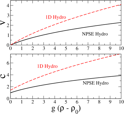
Figure 1: Velocities $v$ and $c$ as a function of the scaled axial density $g\rho$, with $g\rho_{0}=2$. Solid lines: Eqs. (20) and (23). Dashed lines: Eqs. (24) and (25).

In Fig. 1 we plot the velocities $v$ and $c$ as a function of the scaled and shifted axial density $g(\rho-\rho_{0})$, chosing $g\rho_{0}=2$ to enhance the differences between 1D and NPSE hydrodynamics. The solid lines are obtained by using the NPSE hydrodynamics, i.e. Eqs. (20) and (23), while the dashed lines are obtained by using the 1D hydrodynamics, i.e. Eqs. (24) and (25). The two panels clearly show quantitative differerences between 1D and NPSE hydrodynamics. Notice that $v(\rho_{0})=0$ while $c(\rho_{0})=c_{s}(\rho_{0})$.

4 Formation of the shock wave front

Up to now the initial shape of the wave has been arbitrary. We consider now an example by choosing the following initial density profile

$$f(z)=\rho_{0}+\rho_{0}\;\eta\;e^{-z^{2}/(2\sigma)^{2}}\;,$$ (26)

where $\eta$ describes the maximum impulse with respect to the density background $\rho_{0}$. Both amplitude $\mathcal{A}(\eta)$ and velocity $\mathcal{V}(\eta)$ of the impulse maximum are constant during time evolution. The amplitude is $\mathcal{A}(\eta)=\rho_{0}(1+\eta)$ while the velocity reads

$${\mathcal{V}}(\eta)=c(\rho_{0}(1+\eta))\;.$$ (27)

As expected, taking $\eta=0$ the velocity of the impulse maximum reduces to the sound velocity $c(\rho_{0})=c_{s}(\rho_{0})$. Moreover, bright perturbations ($\eta>0$) move faster than dark ones ($\eta<0$) noi2a . Let us consider a bright perturbation. The speed of impulse maximum is bigger than the speed of its tails. As a result the impulse self-steepens in the direction of propagation so that the formation of a shock wave front takes place. The time $T_{s}$ required for such a process can be estimated as follows: the shock wave front appears when the distance difference traveled by lower and upper impulse parts is equal to the impulse half-width $2\sigma$, namely $[{\mathcal{V}}(\eta)-{\mathcal{V}}(0)]T_{s}=2\sigma$. It gives

$$T_{s}={2\sigma\over c(\rho_{0}(1+\eta))-c_{s}(\rho_{0})}\;,$$ (28)

where the local velocity $c(\rho)$ is given by Eq. (23) while the sound velocity $c_{s}(\rho)$ is given by Eq. (8). In the 1D regime ($g\rho\ll 1$) the formula of the time $T_{s}$ reads

$$T_{s}={2\sigma\over 3(\sqrt{1+\eta}-1)\sqrt{g\rho_{0}}}\;.$$ (29)

In the case of a dark perturbation ($\eta<0$) the tails of the wave packet move faster than the impulse minimum and the time of shock formation is simply $T_{s}=2\sigma/(c_{s}(\rho_{0})-c(\rho_{0}(1+\eta))$.

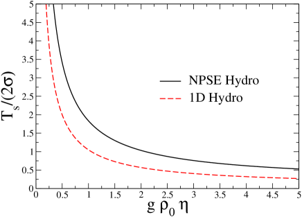
Figure 2: Scaled time of shock formation $T_{s}/(2\sigma)$ as function of the scaled impulse maximum $\rho_{0}\eta$. $\sigma$ is the initial width of the impulse and we set $g\rho_{0}=2$. Solid line: Eq. (28). Dashed line: Eqs. (29).

In Fig. 2 we plot the scaled time $T_{s}/(2\sigma)$ of shock formation as a function of the scaled impulse maximum $\rho_{0}\eta$. Again we choose $g\rho_{0}=2$. The solid line is obtained by using the NPSE hydrodynamics, i.e. Eq. (28), while the dashed line is obtained by using the 1D hydrodynamics, i.e. Eq. (29). Both curves give $T_{s}/(2\sigma)\to+\infty$ as $g\rho_{0}\eta\to 0$.

It is important to stress that our analytical results have been obtained without taking into account the quantum pressure term $1/(2\sqrt{\rho}){\partial^{2}\sqrt{\rho}/\partial z^{2}}$ in Eq. (2). Initially the spatial scale of density variations is $\sigma$, which can be chosen greater than the bulk healing length $\xi(\rho_{0})=(1+g\rho_{0})^{1/2}/\sqrt{2g\rho_{0}}$. As a result the QP term is negligible at the begining of time evolution.

5 Numerical results and after-shock dynamics

As the shock forms up density modulations occur on smaller and smaller length scales beeing finally of the order of the healing length. Damski damski has numerically shown, for the strictly 1D Bose gas, that the effect of quantum pressure term is that of preserving the single-valuedness of the density profile by inducing density oscillations at the shock wave front. Thus, after the formation of the shock Eqs. (1) and (2) are not reliable. To overcome this difficulty we include the dispersive quantum pressure term in the hydrodynamic equations, which become

$${\partial\rho\over\partial t}+{\partial\over\partial z}\left(\rho v\right)=0\;,$$ (30)

$${\partial v\over\partial t}+{\partial\over\partial z}\left({v^{2}\over 2}+\mu(\rho)-{1\over 2\sqrt{\rho}}{\partial^{2}\over\partial z^{2}}\sqrt{\rho}\right)=0\;.$$ (31)

We stress that at zero temperature for a viscousless superfluid the simplest regularization process of the shock is a purely dispersive quantum gradient term, which is proportional to $\hbar^{2}$ in dimensional units. Clearly, Eq. (2) is a first order equation while Eq. (31) is not due to the quantum gradient term.

Introducting the complex field $\psi(z,t)$ such that

$$\psi(z,t)=\sqrt{\rho(z,t)}\,e^{i\theta(z,t)}\;$$ (32)

and

$$v(z,t)={\partial\over\partial z}\theta(z,t)\;.$$ (33)

it is strightforward to show that Eqs. (30) and (31) are equivalent to the following one-dimensional nonlinear Schrödinger equation

$$i{\partial\psi\over\partial t}=\left[-{1\over 2}{\partial^{2}\over\partial z^{2}}+\mu(|\psi|^{2})\right]\psi\;.$$ (34)

Using the bulk chemical potential $\mu(\rho)$ of Eq. (3) with (4), this nonlinear Schrödinger equation is the time-dependent generalized Lieb-Liniger equation we introduced some years ago gll to accurately describe an experiment on a Tonks-Girardeau gas of ⁸⁷Rb atoms weiss . In the BEC regime, where Eq. (3) reduces to Eq. (7), the time-dependent generalized Lieb-liniger equation becomes the 1D time-dependent nonpolynomial Schrödinger equation (NPSE)

$$i{\partial\psi\over\partial t} = \Big{[}-{1\over 2}{\partial^{2}\over\partial z^{2}}+{g|\psi|^{2}\over\sqrt{1+g|\psi|^{2}}}$$

$$+ {1\over 2}\left(\sqrt{1+g|\psi|^{2}}+{1\over\sqrt{1+g|\psi|^{2}}}\right)\Big{]}\psi\;,$$

which gives the familiar one-dimensional Gross-Pitaevskii equation

$$i{\partial\psi\over\partial t} = \Big{[}-{1\over 2}{\partial^{2}\over\partial z^{2}}+g|\psi|^{2}+1\Big{]}\psi\;$$ (36)

in the 1D quasi BEC regime, where $g^{2}\ll g|\psi|^{2}\ll 1$ and the transverse width $\sigma$ of Eq. (4) becomes $\sigma\simeq 1$ (i.e. $\sigma\simeq a_{\bot}$ in dimensional units) npse .

We solve numerically Eq. (5) by using a Crank-Nicolson finite-difference predictor-corrector algorithm sala-numerics with the initial condition given by Eq. (26) and $v(z,t=0)=0$. In fact, as also shown by Damski damski , we have verified that the initial velocity field $v(\rho(z,t=0))$ and $v(z,t=0)=0$ give practically the same time evolution.

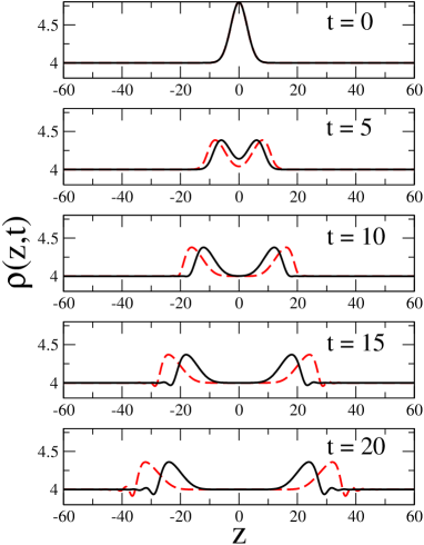
Figure 3: Time evolution of shock waves. Initial condition given by Eq. (26) with $\sigma=4$, $\eta=0.2$ and $\rho_{0}=4$. The curves give the relative density profile $\rho(z,t)$ vs $z$ at subsequent times $t$. Solid lines obtained solving the time-dependent 1D NPSE, Eq. (5), and dashed lines obtained solving the time-dependent 1D GPE, Eq. (36). We choose the nonlinear strength $g=0.5$.

In Fig. 3 we plot the time evolution of shock waves obtained with $\rho_{0}=4$, $\sigma=4$, and $\eta=0.2$. The nonlinear strength is choosen as $g=0.5$, such that $g\rho=2$ and consequently the system is very far from the Tonks-Girardeau regime (characterized by $g\rho\ll g^{2}$). The figure displays the density profile $\rho(z,t)=|\psi(z,t)|^{2}$ at subsequent times. Note the splitting on the initial bright wave packet into two bright travelling waves moving in opposite directions. As previously discussed, there is a deformation of the two waves with the formation of a quasi horizontal shock-wave front. Eventually, this front spreads into dispersive wave ripples. The figure shows that there is no qualitative difference between 1D NPSE (solid lines) and 1D GPE (dashed lines) in the physical manifestation of supersonic shock waves. Nevertheless, due to the different equation of state, there are quantitative differences. Our numerical simulation confirms that the velocity of the maximum of the shock wave is larger for the 1D GPE with respect to the 1D NPSE.

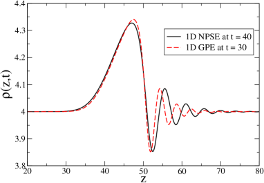
Figure 4: Zoom of the density profile $\rho(z,t)$ vs $z$ of the shock wave. Initial condition given by Eq. (26) with $\sigma=4$, $\eta=0.2$ and $\rho_{0}=4$. Solid line obtained solving the time-dependent 1D NPSE, Eq. (5) at $t=40$, and dashed line obtained solving the time-dependent 1D GPE, Eq. (36) at $t=30$. We choose the nonlinear strength $g=0.5$.

In Fig. 4 we plot a zoom of the density profile $\rho(z,t)$ of the shock wave to better show the after-shock dispersive ripples. In the figure we compare the density profiles obtained with 1D NPSE and 3D GPE by chosing $t=30$ for 1D GPE and $t=40$ for 1D NPSE: in this way the spatial position of the highest maxima of the two profiles is practically superimposed. Fig. 4 clearly shows that the wavelength of the dispersive ripples is larger in the case of the 1D NPSE. We have verifed that this is a general feature by performing other numerical runs with different initial conditions.

6 Conclusions

We have shown that the shock-wave dynamics (velocity and density ripples) in a quasi 1D BEC, described by the 1D nonpolynomial Schrödinger equation (NPSE), is quite different with respect to the shock-wave dynamics of a strictly-1D BEC, described by the 1D Gross-Pitaevskii equation (GPE). The dynamics of the quasi 1D BEC becomes becomes equivalent to the one of the strictly-1D BEC only under the condition $g\rho\ll 1$, with $g$ the interaction strength and $\rho$ the one-dimensional axial density. In particular we have found that by using 1D NPSE the maximum of the shock wave moves slower, the time of shock formation is longer, and dispersive ripples have larger wavelength with respect to 1D GPE. For both 1D NPSE and 1D GPE we have obtained analytical and numerical solutions which could be compared with experimental data. Indeed, shock waves can be experimentally produced by engineering the initial density of the superfluid. Working with BECs made of alkali-metal atoms and confined in the transverse direction by a blue-detuned axial laser beam, a choosen axial density profile can be obtained by using a blue-detuned (bright perturbation) or a red-detuned (dark perturbation) laser beam perpendicular to the longitudinal axial direction. In this way one can experimentally test the equation of state of the quasi one-dimensional Bose-Einstein condensate analyzing the dynamical properties of the generated shock waves.

References

- (1) L.D. Landau and E.M. Lifshitz, Fluid Mechanics, chapt. 10, par. 101 (Pergamon Press, London, 1987).
- (2) L.P. Pitaevskii and S. Stringari, Bose-Einstein Condensation (Oxford Univ. Press, Oxford, 2003).
- (3) S. Giorgini, L.P. Pitaevskii, and S. Stringari, Rev. Mod. Phys. 80, 1215 (2008).
- (4) L. Salasnich and F. Toigo, Phys. Rev. A 78, 053626 (2008); L. Salasnich, Laser Phys. 19, 642 (2009).
- (5) Z. Dutton, M. Budde, C. Slowe, and L.V. Hau, Science 293, 663 (2001).
- (6) M.A. Hoefer, M.J. Ablowitz, I. Coddington, E.A. Cornell, P. Engels, and V. Schweikhard, Phys. Rev. A 74, 023623 (2006).
- (7) J.J. Chang, P. Engels, and M.A. Hoefer, Phys. Rev. Lett. 101, 170404 (2008).
- (8) R. Meppelink, S.B. Koller, J.M. Vogels, P. van der Straten, E.D. van Ooijen, N.R. Heckenberg, H. Rubinszein-Dunlop, S.A. Haine, and M.J. Davis, Phys. Rev. A 80, 043606 (2009).
- (9) J.A. Joseph, J.E. Thomas, M. Kulkarni, and A.G. Abanov A G, Phys. Rev. Lett. 106, 150401 (2011).
- (10) I. Kulikov and M. Zak, Phys. Rev. A 67, 063605 (2003).
- (11) B. Damski, Phys. Rev. A 69, 043610 (2004); B. Damski, Phys. Rev. A 73, 043601 (2006).
- (12) A.M. Kamchatnov, A. Gammal, and R.A. Kraenkel, Phys. Rev. A 69, 063605 (2004).
- (13) V.M. Perez-Garcia, V.V. Konotop, and V.A. Brazhnyi, Phys. Rev. Lett. 92, 220403 (2004).
- (14) A. Ruschhaupt, A. del Campo, and J.G. Muga, Eur. Phys. J. D 40, 399 (2006).
- (15) L. Salasnich, N. Manini, F. Bonelli, M. Korbman, and A. Parola, Phys. Rev. A 75, 043616 (2007).
- (16) L. Salasnich, EPL 96, 40007 (2011).
- (17) F. Ancilotto, L. Salasnich, and F. Toigo, Phys. Rev. A 85, 063612 (2012); L. Salasnich, Few Body Sys. 54, 697 (2013).
- (18) A. Bulgac, Y-L. Luo, and K.J. Roche, Phys. Rev. Lett. 108, 150401 (2012).
- (19) L. Salasnich, Laser Phys. 12, 198 (2002); L. Salasnich, A. Parola, and L. Reatto, Phys. Rev. A 65, 043614 (2002); L. Salasnich, J. Phys. A: Math. Theor. 42, 335205 (2009).
- (20) L. Salasnich, A. Parola, and L. Reatto, Phys. Rev. A 70, 013606 (2004); L. Salasnich, A. Parola, and L. Reatto, Phys. Rev. A 72, 025602 (2005).
- (21) E.H. Lieb and W. Liniger, Phys. Rev. 130, 1605 (1963).
- (22) M. Girardeau, J. Math. Phys. 1, 516 (1960).
- (23) A. Munoz Mateo and V. Delgado, Phys. Rev. A 75, 063610 (2007); A. Munoz Mateo and V. Delgado, Phys. Rev. A 77, 013617 (2008); A. Munoz Mateo and V. Delgado, Ann. Phys. 324, 709 (2009).
- (24) A.M. Kamchatnov and V.S. Shchesnovich, Phys. Rev. A 70, 023604 (2004).
- (25) L. Salasnich, Int. J. Mod. Phys. B 14, 1 (2000).
- (26) P. Massignan and M. Modugno, Phys. Rev. A 67, 023614 (2003); M. Modugno, C. Tozzo, and F. Dalfovo, Phys. Rev. A 70, 043625 (2004); C. Tozzo, C.M. Kramer, and F. Dalfovo, Phys. Rev. A 72, 023613 (2005); M. Modugno, Phys. Rev. A 73, 013606 (2006).
- (27) G. Theocharis, P.G. Kevrekidis, M.K. Oberthaler, and D.J. Frantzeskakis, Phys. Rev. A 76, 045601 (2007); A. Weller, J.P. Ronzheimer, C. Gross, J. Esteve, M.K. Oberthaler, D.J. Frantzeskakis, G. Theocharis, and P.G. Kevrekidis, Phys. Rev. Lett. 101, 130401 (2008).
- (28) G. Mazzarella and L. Salasnich, Phys. Rev. A 82, 033611 (2010).
- (29) G Mazzarella, M Moratti, L Salasnich, M Salerno, and F Toigo, J. Phys. B: At. Mol. Opt. Phys. 42, 125301 (2009); G. Mazzarella, L. Salasnich, A. Parola, and F. Toigo, Phys. Rev. A 83, 053607 (2011).
- (30) L. Salasnich, A. Parola, and L. Reatto, Phys. Rev. A 69, 045601 (2004).
- (31) S. Burger et al., Phys. Rev. Lett. 83, 5198 (1999); J. Denschlag et al., Science 287, 97 (2000).
- (32) T. Kinoshita, T. Wenger, and D.S. Weiss, Science 305, 1125 (2004).
- (33) E. Cerboneschi, R. Mannella, E. Arimondo, and L. Salasnich, Phys. Lett. A 249, 495 (1998); G. Mazzarella and L. Salasnich, Phys. Lett. A 373 4434 (2009).