Decode-Forward Transmission for the Two-Way Relay Channels

Abstract

We propose composite decode-forward (DF) schemes for the two-way relay channel in both the full- and half-duplex modes by combining coherent relaying, independent relaying and partial relaying strategies. For the full-duplex mode, the relay partially decodes each user’s information in each block and forwards this partial information coherently with the source user to the destination user in the next block as in block Markov coding. In addition, the relay independently broadcasts a binning index of both users’ decoded information parts in the next block as in independent network coding. Each technique has a different impact on the relay power usage and the rate region. We further analyze in detail the independent partial DF scheme and derive in closed-form link regimes when this scheme achieves a strictly larger rate region than just time-sharing between its constituent techniques, direct transmission and independent DF relaying, and when it reduces to a simpler scheme. For the half-duplex mode, we propose a $6$-phase time-division scheme that incorporates all considered relaying techniques and uses joint decoding simultaneously over all receiving phases. Numerical results show significant rate gains over existing DF schemes, obtained by performing link adaptation of the composite scheme based on the identified link regimes.

I Introduction

The two-way relay channel (TWRC) has received attention as one of the basic cooperation models in both wired and wireless networks. The existence of different routes in a wired network or the shared-medium nature of a wireless network allows a relay node to help exchange information between two source nodes. The application is apparent in infrastructure-less networks such as ad hoc and sensor networks, where two nodes can communicate with help from a third node in between. In infrastructure-aided networks such as the cellular system, the newly introduced device-to-device communication mode [1] also allows the application of two-way relay transmission, where the relay could be an idle user or a nearby femto base station helping the direct communication between two active users. Such a scenario is appealing in high speed video exchange for example.

Multiple two-way relaying strategies have been proposed for both full- and half-duplex communications [2, 3, 4, 5, 6, 7, 8, 9, 10], each strategy has slightly different rate region performance from the others. On the one hand, it is of theoretical interest to find a composite scheme that achieves the highest performance and includes all known schemes. On the other hand, it is of practical interest to design the simplest scheme that achieves the maximum performance. These seemingly contradicting interests require a thorough understanding of the effect on performance of each separate relaying strategy and the condition for this effect to be maximized. Such a condition may appear in the form of regimes on the network links strength. The more complicated scheme is then only needed under specific link regimes. Mapping out these link regimes is related to the optimal resource allocation to the constituent techniques in a composite scheme, but the question here is not to find the exact optimal resource allocation to all techniques, but to ask when it is optimal to allocate zero resources to a certain technique (so that the optimal scheme need not use that technique). This topic has not been explored much in the literature.

I-A Related works

Several full-duplex schemes have been proposed for the TWRC, differing mainly on the relaying techniques employed at the relay. Inspired by the basic techniques for the classical one-way relay channel [11], different decode-and-forward and compress-and-forward relaying schemes have been applied to the TWRC. In this paper, we focus on the decode-and-forward (DF) strategies where the relay fully or partially decodes the information of each user and forwards it to the other user in the next transmission block. A DF strategy based on block Markov encoding is proposed in [2], where in each transmission block, both users send their new information and also repeat the old information of the previous block. Different from the regular one-way relay channel, here each user’s old information is sent coherently with only a part of the relay’s transmit signal, but not with the whole relay signal, which contains information of both users and is unknown at either user. In another DF strategy without block Markovity [3], the users do not repeat their old messages and the relay forwards only an independent codeword as a function of both users’ messages without coherent transmission with either user. This independent coding strategy resembles the idea of network coding at the relay. Each of these two strategies has a different impact on the achievable rate and the power allocation at the relay; neither strategy always outperforms the other one.

Partial DF (pDF) relaying has not been investigated much in the literature, except when it is in combination with another relaying strategy such as compress-and-forward [12]. This is most likely because of the belief that partial DF alone does not bring improvement over full DF relaying as in the classical single-antenna one-way relay channel [13]. Rather surprisingly, we showed that for the two-way relay channel, partial DF can strictly improve performance over full DF [6]. The improvement comes from the fact that signals from multiple users can now interfere with each other, hence in certain link regimes, it is better to reduce this interference by performing decode-and-forward partially.

For the half-duplex mode, existing works differ mainly in the number of phases, the relaying technique at the relay, and the decoding technique at the users. A $4$-phase independent DF is proposed in [5] where the two users alternatively transmits and receives during the first two phases, both users transmit in phase $3$ and the relay transmits in phase $4$. The most general strategy for half-duplex TWRC includes $6$ phases, which has been considered in several works including [7, 8], where in each of the additional $2$ phases, one user and the relay independently transmit to the other user. The degrees of freedom is analyzed for a $6$-phase independent DF scheme with multiple-antenna nodes in [9]. Another $6$-phase scheme considering both independent and coherent pDF relaying is proposed in [10], where coherent transmissions occur in phases $5$ and $6$. However, the users perform separate decoding at the end of each phase instead of simultaneous decoding over all phases.

Although many schemes have been proposed for the TWRC, few works analyzed them. Most existing analysis is about the optimal resource allocation for a simple scheme. For example, a $2$-phase half-duplex DF scheme without the direct links between users is optimized for the phase durations to maximize the rate region [14] and the sum rate [15]. An OFDMA $2$-phase DF scheme is optimized for the resource allocations that achieve the largest achievable rate region per OFDMA subcarrier [16] or jointly over all multi-carriers [17]. Analysis for more complex schemes which are composed of several techniques is not yet seen in the literature.

I-B Main results and contributions

In this paper, we investigate a composite scheme for the TWRC based on decode-and-forward relaying that includes several techniques: coherent block Markov relaying, independent relaying, and partial relaying. Such a combination of DF techniques has not been considered previously in the literature. We design and analyze the composite schemes in both the full- and half-duplex modes. The full-duplex design allows a detailed analysis on the performance impact of the considered techniques under different link regimes, whereas the half-duplex adaptation allows application in current wireless systems.

In our proposed schemes, each user splits its message into a common and a private part, the common message is to be decoded at the relay, whereas the private message is to be decoded only at the destination. For full-duplex transmission, each user superposes its private part over the common part of the current block and the common part of the previous block. The relay decodes the current common messages of both users and forward each previous common message coherently with its source user to the destination user. In addition, the relay encodes a bin index that is a function of both users’ common messages and forwards it independently with the signals from the users. The relay’s signal therefore is a superposition of three parts. Each user employs sliding window decoding over two consecutive blocks to decode the other user’s messages. This scheme is a generalization of our previous schemes in conference publications [4, 6]; it also includes all existing schemes in [2, 3] as special cases and achieves a strictly larger rate region than the time-shared region between these schemes.

We then analyze in detail the independent coding and partial DF relaying components of our scheme to understand when each of these constituent techniques is necessary. Without one or both these techniques, the scheme reduces to two-way full DF relaying, direct transmission or a hybrid one-way full DF relaying for one user and direct transmission for the other user. We derive conditions on link strengths for when it is sufficient to use one of these simplified schemes to achieve the maximum achievable rate region and when it is necessary to perform the composite independent partial DF. Such a link-regime identification has not been done before, and provides the necessary insights for applying two-way relaying in practice. These link regimes also reveal that independent partial relaying is beneficial in the TWRC when the relay link from one user is slightly stronger than its direct link, quantified by conditions among the received SNRs over these links. Because of space and complexity constraints, link-regime analysis is performed separately for the independent and coherent full DF relaying components in [18].

For the half-duplex mode, we propose an inclusive $6$-phase time-division scheme. Different from existing $6$-phase schemes [7, 8, 9, 10], our scheme utilize all coherent, independent and partial relaying techniques; furthermore, both users employ simultaneous decoding over all phases instead of separate decoding in each phase. Hence, our scheme outperforms all existing schemes.

The rest of this paper is organized as follows. Section II describes the TWRC model for both the full- and half-duplex modes. Section III describes the proposed composite pDF scheme for the full-duplex mode and derives its achievable rate region. Section IV analyzes the link regimes for the independent pDF scheme. Section V describes an inclusive $6$-phase pDF scheme for the half-duplex mode. Section VI presents numerical results and Section VII concludes the paper.

II Two-way relay channel model

The two-way relay channel consists of two user nodes, each with its own information to send to the other node, and a relay node that can receive from and transmit to both user nodes to facilitate communication between them. We are interested in the full TWRC with a direct link between the two user nodes in addition to the links to the relay which captures the full interaction in a wireless environment.

Next we will present both full and half-duplex channel models as shown in Figure 1. Traditionally, wireless communication devices are half-duplex, meaning that they can only transmit or only receive on a single frequency band at a time. Recently, full-duplex wireless has been demonstrated to work even with just a single transmit and a single receive antenna, bringing the possibility of functional full-duplex wireless systems in the future. In this paper, we will analyze both the full and half-duplex modes for the TWRC. Often the design and properties of a transmission scheme for the full-duplex mode can be applied to the half-duplex mode. Hence considering both modes helps us focus on the design and analysis of transmission schemes for the full-duplex mode first, then extend these schemes to satisfy the half-duplex constraint.

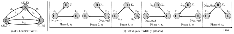
Figure 1: Full and Half-duplex model for TWRC.

II-A Full-duplex channel model

The full-duplex TWRC as shown in Figure 1(a) can be modeled as

$$Y_{1} =h_{12}X_{2}+h_{1r}X_{r}+Z_{1},$$

$$Y_{2} =h_{21}X_{1}+h_{2r}X_{r}+Z_{2},$$

$$Y_{r} =h_{r1}X_{1}+h_{r2}X_{2}+Z_{r},$$ (1)

where $Z_{1},Z_{2},Z_{r}\sim\mathcal{CN}(0,1)$ are independent complex Gaussian noises with zero mean and unit variance, and $(X_{1},Y_{1})$, $(X_{2},Y_{2})$, $(X_{r},Y_{r})$ are pairs of the transmitted signal and received signal at user $1$ $(\mathbf{U}_{1})$, user $2$ $(\mathbf{U}_{2})$ and the relay, respectively. The average input power constraints for $\mathbf{U}_{1}$, $\mathbf{U}_{2}$ and the relay are assumed to be $P_{1},$ $P_{2}$ and $P_{r}$, respectively.

The channel gain coefficients $h_{12},h_{1r},h_{21},h_{2r},h_{r1},h_{r2}$ are complex value. We use the standard assumption in coherent relaying literature [11, 13, 19] that the phases of these channel coefficients are known at the respective transmitters so that coherent transmission from two different transmitters are possible, and the full channel coefficients are known at the respective receivers. As such, the achievable rate will depend only on the amplitude of the channel coefficients, which we will denote as $g$ with the same subscripts as $h$.

II-B Half-duplex channel model

Time division is used to adapt a full-duplex transmission scheme to the half-duplex mode. The main idea is that each transmission block, (or equivalently a time slot or a frame) is divided into several phases. Depending on the number of phases, different half-duplex protocols can result. Existing literature has a number of variation with $2$, $3$, $4$ or $6$ phases [5, 6, 7, 8, 9, 10].

In this paper, we will consider the most comprehensive and inclusive $6$-phase protocol. The $6$-phase protocol encompasses all other half-duplex protocols as special cases, which can be obtained by setting the duration of some of the $6$ phases to zero. The channel model for each phase, as depicted in Figure 1(b), can be expressed as

$$\!\!\!\!\text{Phase 1:}\;Y_{21} =h_{21}X_{11}+Z_{21},\;Y_{r1}=h_{r1}X_{11}+Z_{r1},$$

$$\!\!\!\!\text{Phase 2:}\;Y_{12} =h_{12}X_{22}+Z_{12},\;Y_{r2}=h_{r2}X_{22}+Z_{r2},$$

$$\!\!\!\!\text{Phase 3:}\;Y_{r3} =h_{r1}X_{13}+h_{r2}X_{23}+Z_{r3},$$

$$\!\!\!\!\text{Phase 4:}\;Y_{24} =h_{21}X_{14}+h_{2r}X_{r4}+Z_{24},$$

$$\!\!\!\!\text{Phase 5:}\;Y_{15} =h_{12}X_{25}+h_{1r}X_{r5}+Z_{15},$$

$$\!\!\!\!\text{Phase 6:}\;Y_{16} =h_{1r}X_{r6}+Z_{16},\;Y_{26}=h_{2r}X_{r6}+Z_{26},$$ (2)

where $X_{ij}$ and $Y_{ij}$, ($i\in[1,2,r],j\in[1,\ldots,6]$) respectively represents the transmitted and received signal of user $i$ during phase $j$. All the noises $Z_{ij}$ are i.i.d $\sim\mathcal{CN}(0,1).$ The channel coefficients are similarly defined as in the full-duplex model.

III A full-duplex decode-forward transmission scheme

The unique feature in designing a DF scheme for the TWRC arises from the fact that each user does not have the complete information decoded at the relay, as was the case in the one-way relay channel. There are two different ways to build a DF scheme for the TWRC, depending on whether the source performs block Markov encoding on only a part of the relay’s signal, or performs coding independently with the relay. Further, partial DF has not been previously considered for the TWRC but can strictly outperform full DF, as shown later in this paper. Next, we propose a new composite pDF scheme for the TWRC that combines all three strategies: partial DF, coherent block Markov coding and independent coding.

III-A Transmission scheme

Each user node splits its message into two parts: a common message and a private message. The user first encodes the common message by superposing this message on the common message of the previous block as in block Markov coding; it then superposes the private message on the current common message. The relay only decodes the current common message of each user; it then performs random binning of the pair of decoded common messages and generates a codeword for this bin index, superposes this codeword on the two codewords for two common messages, effectively combining relay strategies of both [3] and [2]. The relay forwards this codeword containing the two decoded common messages and their bin index in the next block. Each user decodes the other user’s message by sliding window decoding based on received signals in both the current and previous blocks.

III-A1 Transmit signal design

Denote the new messages user 1 and user 2 send in block $i$ as $m_{1,i}$ and $m_{2,i}$, respectively. Each user splits its own message as $m_{1,i}=(m_{10,i},m_{11,i})$ and $m_{2,i}=(m_{20,i},m_{22,i})$, where the first part is the common message and the second is the private message. The relay partitions the set of all common messages $\{m_{10,i-1},m_{20,i-1}\}$ equally and uniformly into a number of bins and indexes these bins by $\{l_{i-1}\}$. The users and the relay then construct the transmit signals in block $i$ as follows:

$$X_{1} =\sqrt{\alpha_{1}}W_{1}(m_{10,i-1})+\sqrt{\beta_{1}}U_{1}(m_{10,i})+\sqrt{\gamma_{1}}Q_{1}(m_{11,i})$$

$$X_{2} =\sqrt{\alpha_{2}}W_{2}(m_{20,i-1})+\sqrt{\beta_{2}}U_{2}(m_{20,i})+\sqrt{\gamma_{2}}Q_{2}(m_{22,i})$$

$$X_{r} =\sqrt{k_{1}\alpha_{1}}W_{1}(m_{10,i-1})+\sqrt{k_{2}\alpha_{2}}W_{2}(m_{20,i-1})$$

$$\;\;+\sqrt{\beta_{3}}U_{r}(l_{i-1})$$ (3)

where $W_{1},W_{2},U_{1},U_{2},U_{r},Q_{1},Q_{2}$ are independent Gaussian signals with zero mean and unit variance that encode the respective messages and bin index. Power allocation factors $\alpha_{1},\alpha_{2},\beta_{1},\beta_{2},\beta_{3},$ $\gamma_{1},\gamma_{2}$ are non-negative and satisfy

$$\alpha_{1}+\beta_{1}+\gamma_{1} \leq P_{1},$$

$$\alpha_{2}+\beta_{2}+\gamma_{2} \leq P_{2},$$

$$k_{1}\alpha_{1}+k_{2}\alpha_{2}+\beta_{3} \leq P_{r},$$ (4)

where $k_{1},k_{2}$ are scaling factors that relate the power allocated to transmit the same common message at each user and the relay.

We note several features of the signal construction in (3). In each transmission block, each user sends not only new messages of that block (with index $i$), but also repeats the common message of the previous block (with index $i-1$). The relay always transmits information of the previous block which it decodes only at the end of the previous block. Thus the block Markov structure creates a coherency between the common signal parts transmitted from each user and the relay (denoted by $W_{1}$ and $W_{2}$) which results in a beamforming gain.

The relay not only forwards the signals $W_{1}$ and $W_{2}$ but also creates a new signal $U_{r}$ that independently encodes both common messages via binning. The random binning is a function of both messages decoded at the relay and resembles network coding.

Each of these two relaying strategies has a unique implication. Markov block coding brings a coherent beamforming gain between a source and the relay, but requires the relay to split its power between $W_{1}$ and $W_{2}$ for each pair of common messages. Independent network coding via binning, on the other hand, let the relay use its whole power to send the bin index of the message pair. This bin index can then solely represent one common message when decoding at each user because of side information on the other common message available at this user, as can be seen in the decoding discussion below.

III-A2 Decoding rules

Decoding occurs at all nodes, including the relay and the users. We assume all messages are equally likely and all nodes use maximum likelihood (ML) sequence detection, which in this case is equivalent to the optimal decoding rule presented next.

At the relay, decoding is quite simple and is similar to decoding in the multiple access channel. The received signal in block $i$ at the relay is

$$Y_{r} =h_{r1}\left(\sqrt{\alpha_{1}}W_{1}+\sqrt{\beta_{1}}U_{1}+\sqrt{\gamma_{1}}Q_{1}\right)$$ (5)

$$\;\;+h_{r2}\left(\sqrt{\alpha_{2}}W_{2}+\sqrt{\beta_{2}}U_{2}+\sqrt{\gamma_{2}}Q_{2}\right)+Z_{r}.$$

In block $i$, the relay already knows $W_{1},W_{2}$ (which carry $m_{10,i-1},m_{20,i-1}$) and is interested in decoding ${U}_{1}$ and ${U}_{2}$ (which carry $m_{10,i},m_{20,i}$). For the purpose of highlighting what is known, we write the optimal maximum a posteriori probability (MAP) decoding rule, which can be converted to ML decoding rule, as

$$\left(m_{10,i},m_{20,i}\right)=\arg\max P(U_{1,i},U_{2,i}|Y_{r,i},W_{1,i},W_{2,i}).$$ (6)

In this decoding, the relay treats signals ($Q_{1},Q_{2}$) that carry the private information as noise.

Decoding at each user node is based on signals received in two consecutive blocks. To decode new information sent in block $i$, a user will use received signals in both blocks $i$ and $i+1$, which results in a one-block decoding delay. Take user 2 for example, this user’s received signal in each block is

$$Y_{2} =h_{21}\left(\sqrt{\alpha_{1}}W_{1}+\sqrt{\beta_{1}}U_{1}+\sqrt{\gamma_{1}}Q_{1}\right)$$ (7)

$$\;\;+h_{2r}\left(\sqrt{k_{1}\alpha_{1}}W_{1}+\sqrt{k_{2}\alpha_{2}}W_{2}+\sqrt{\beta_{3}}U_{r}\right)+Z_{2}.$$

User 2 knows its own signal $W_{2}$ and can directly subtract it from the received signal.

At the end block $i$, each user has presumably decoded all previous blocks information correctly. That means in block $i$, user 2 knows $W_{1},U_{r}$ (which encode $w_{10,i-1}$) and thus only needs to decode $U_{1},Q_{1}$ (which encode $w_{10,i},w_{11,i}$). In block $i+1$, the relevant signals carrying the same wanted information are $W_{1}$ and $U_{r}$ (which encode $w_{10,i}$). Note that even though $U_{r}$ encodes the bin index of the pair of common messages and hence carries information about both common messages, but because one common message is originated and thus is known at each user, $U_{r}$ can be used at each user solely to decode the other common message. This is the effect of side information in decoding at each user in the TWRC, which has also been noted in [5]. For block $i+1$, user 2 will decode $W_{1}$ and $U_{r}$ while treating the other signals $U_{1},Q_{1}$ as noise.

We write this joint decoding over two blocks using MAP decoding at user 2 as follows:

$$\left(m_{10,i},m_{11,i}\right)=\arg\max\big{(}P(U_{1,i},Q_{1,i}|Y_{2,i},W_{2,i},W_{1,i},U_{r,i})$$

$$\times P(W_{1,i+1},U_{r,i+1}|Y_{2,i+1},W_{2,i+1},m_{20,i}\big{)}.$$ (8)

Note that the above decoding rule applies across two blocks simultaneously, such that the decoded message pair maximizes the product of the decoding probabilities in these blocks.

III-B Achievable rate region

With above scheme, we get the following achievable rate region.

Theorem 1.

Using the proposed partial decode-forward based scheme, the following rate region is achievable for the Gaussian two-way relay channel:

$$R_{1} \leq\min\{I_{1}+I_{4},I_{5}\},$$

$$R_{2} \leq\min\{I_{2}+I_{6},I_{7}\},$$

$$R_{1}+R_{2} \leq I_{3}+I_{4}+I_{6},\;\;\text{where}$$ (9)

$$I_{1} =C\left(\frac{g_{r1}^{2}\beta_{1}}{g_{r1}^{2}\gamma_{1}+g_{r2}^{2}\gamma_{2}+1}\right),\quad I_{4}=C(g_{21}^{2}\gamma_{1}),$$ (10)

$$I_{2} =C\left(\frac{g_{r2}^{2}\beta_{2}}{g_{r1}^{2}\gamma_{1}+g_{r2}^{2}\gamma_{2}+1}\right),\quad I_{6}=C(g_{12}^{2}\gamma_{2}),$$

$$I_{3} =C\left(\frac{g_{r1}^{2}\beta_{1}+g_{r2}^{2}\beta_{2}}{g_{r1}^{2}\gamma_{1}+g_{r2}^{2}\gamma_{2}+1}\right),$$

$$I_{5} =C\left(\alpha_{1}\left(g_{21}+g_{2r}\sqrt{k_{1}}\right)^{2}+g_{21}^{2}(\beta_{1}+\gamma_{1})+g_{2r}^{2}\beta_{3}\right)$$

$$I_{7} =C\left(\alpha_{2}\left(g_{12}+g_{1r}\sqrt{k_{2}}\right)^{2}+g_{12}^{2}(\beta_{2}+\gamma_{2})+g_{1r}^{2}\beta_{3}\right),$$

with $C(x)=\log(x+1)$, $g_{*}=|h_{*}|$ as amplitudes of $h_{*}$, and power factors satisfying (4).

Proof:

To sketch the main ideas, rate constraints $I_{1},I_{2},I_{3}$ come directly from decoding the common messages at the relay as in a multiple access channel. Constraints $I_{4}$ and $I_{6}$ come from decoding the private messages at each user, assuming the common messages have been decoded correctly as at the relay. Constraints $I_{5}$ and $I_{7}$ come from the joint decoding of both common and private messages at a user. As such, the transmission rate of each user (which is the sum of the common and private message rates) is constrained by the smaller of the two rates achievable by decoding at the other user only, and across the relay and the other user. A rigorous proof based on information theoretic analysis is available in Appendix A. ∎

The expressions $I_{5}$ and $I_{7}$ carry several important features that are direct results of the signal structure at the relay. Recall that the signal at the relay in (3) contains two parts: the block Markov parts in $W_{1},W_{2}$ and the independent part in $U_{r}$. The block Markov parts contribute to a coherent beamforming gain in $I_{5}$ and $I_{7}$. The power allocated to the beamforming signals is separate in $k_{1}\alpha_{1}$ and $k_{2}\alpha_{2}$, where each part contributes to the achievable rate of only one user (either $R_{1}$ or $R_{2}$). On the other hand, the independent signal part has power $\beta_{3}$ that contributes to the rates of both users (both $R_{1}$ and $R_{2}$). Hence there is an interesting balance in allocating power to each signal part at the relay as to maximize the rate region, where beamforming has higher rate but requires a power split at the relay, and independent signaling has lower rate but can use the whole power to increase the transmission rate of each user.

By adjusting the power allocation, the proposed scheme encompasses and improves upon all previous DF-based schemes [2, 3]. Specifically, the proposed scheme reduces to the Markov (coherent) DF scheme in [2] by setting $\gamma_{1}=\gamma_{2}=\beta_{3}=0$; to the independent DF scheme in [3] by setting $\alpha_{1}=\alpha_{2}=\gamma_{1}=\gamma_{2}=0$; and to the DT scheme by setting $\alpha_{1}=\alpha_{2}=\beta_{1}=\beta_{2}=\beta_{3}=0$. Moreover, by setting $\gamma_{1}=\alpha_{2}=\beta_{2}=0$, the proposed scheme reduces to the hybrid DF and DT scheme where user $1$ performs coherent and independent DF relaying with the relay while user $2$ performs DT. By further setting $\beta_{3}=0$ ($\alpha_{1}=0)$, the scheme has user $1$ performs only coherent (independent) DF relaying with the relay. By setting $\gamma_{2}=\alpha_{1}=\beta_{1}=0$, we have the opposite of the previous case where user $1$ performs DT and user $2$ performs DF relaying.

As shown later in both analysis and simulation, however, the proposed scheme performance is not a mere linear combination of the existing schemes performance. Our scheme can outperform all existing schemes and their combination by achieving rate points outside the time-sharing region of existing schemes.

IV Analysis of the full-duplex scheme

We have proposed a composite DF scheme for the TWRC that utilizes several techniques: coherent block Markov coding, independent coding and partial forwarding. Each technique is represented by a signal part in the proposed transmit signal structure at each node. When a technique is not needed, its associated signal part will be allocated zero power. The necessity of each of these techniques depends on the network configuration, in particular the relative strength of different links in the network. For some link regimes, the proposed scheme can reduce to a simpler scheme without using certain techniques and still achieve the maximum rates, while for other link regimes, all techniques are necessary in order to achieve the largest rate region. It is of important practical value to be able to map out these link regimes precisely and understand which techniques are required in each regime. These link regimes can serve as a basis for performing link adaptation of the composite scheme, depending on the available channel state information. Specifically, the transmitters only need to know certain relative order of the link strengths in order to determine what combination of techniques is optimal.

Mapping out these link regimes analytically is challenging. It is mainly because the associated rate region optimization problem contains multiple variables and, in general, is non-convex. In order to simplify the analysis, in this paper, we focus only on a subset of the considered techniques including the partial DF relaying and independent coding. Analyzing block Markov coding with independent coding is done separately in [20, 18], and the synthesis of all three techniques is left as a future work.

IV-A Link regimes of partial decode-forward with independent relay coding

For this analysis, we consider only independent coding and partial relaying. Each user splits its message into two parts, the relay decodes only one part – the common message – from each user, then puts the decoded message pair into a corresponding bin and forwards the bin index in the next block. The relay effectively performs network coding where the signal from the relay contains the common messages of both users but is independent of signals from both users. While there is no coherent beamforming gain between the relay and each user, the total relay transmit power is effectively allocated to carry the common message of only one user, since the other common message is already known at the decoding user.

This independent pDF scheme can be viewed as a combination of DF relaying (of the common message parts) and direct transmission (of the private message parts). For the standard one-way Gaussian relay channel with single antenna at each node, DF relaying is known to be more useful than direct transmission only if the source-relay link is stronger than the source-destination link. Furthermore, pDF performs no better than DF relaying [13]. The main reason is the power split required to transmit two different information parts at the source. If the source-relay link is stronger than the direct link, then it is more beneficial to put all power into the signal part to be decoded via the source-relay link, practically leading to no message splitting nor partial DF.

For the TWRC, is partial DF any better than full DF, and is it more than just a mere linear (time-shared) combination of full DF and direct transmission? We find that the answers to these questions are both positive. Indeed independent pDF can outperform full DF and achieve rate points strictly outside the DF-DT time-shared region under certain link conditions.

To obtain this result, we analyze the rate region in (10) directly, after setting $\alpha_{1}=\alpha_{2}=0$ (no block Markov coding). The scheme reduces to full DF when the optimal solution is $\gamma_{1}^{\star}=\gamma_{2}^{\star}=0$, and to direct transmission (DT) when $\beta_{1}^{\star}=\beta_{2}^{\star}=0$. When neither case holds, partial DF relaying is used. The results are summarized next.

Theorem 2.

The independent partial DF (pDF) scheme can be optimally divided into several operating regimes depending on the link states as follows.

1. One user performs pDF and the other user switches between DT and full DF when

   $$g_{21}^{2} <g_{r1}^{2}<\left(g_{21}^{2}+g_{2r}^{2}\frac{P_{r}}{P_{1}}\right)(1+g_{r2}^{2}P_{2}),$$

   $$\text{and}\quad g_{r2}^{2}<g_{12}^{2},$$ (11a)

   $$\text{or}\quad g_{12}^{2} <g_{r2}^{2}<\left(g_{12}^{2}+g_{1r}^{2}\frac{P_{r}}{P_{2}}\right)(1+g_{r1}^{2}P_{1}),$$

   $$\text{and}\quad g_{r1}^{2}<g_{21}^{2}.$$ (11b)

   This regime further contains two sub-regimes. The sub-regime in which the pDF scheme achieves the time-shared region between DF and DT is specified by

   $$\!\!\!\!\!\!\!\!\!\!\!\!g_{21}^{2} <g_{r1}^{2}<\min\left\{\left(g_{21}^{2}+g_{2r}^{2}\frac{P_{r}}{P_{1}}\right),\;g_{21}^{2}(1+g_{r2}^{2}P_{2})\right\},\;$$

   $$g_{r2}^{2}<g_{12}^{2},\;\text{and}\;R_{S,1}\leq R_{TS,1}$$ (12a)

   $$\!\!\!\!\!\!\!\!\!\!\!\!\text{or}\;g_{12}^{2} <g_{r2}^{2}<\min\left\{\left(g_{12}^{2}+g_{1r}^{2}\frac{P_{r}}{P_{2}}\right),\;g_{12}^{2}(1+g_{r1}^{2}P_{1})\right\},$$

   $$g_{r1}^{2}<g_{21}^{2},\;\text{and}\;R_{S,2}\leq R_{TS,2}$$ (12b)

   where $R_{S,i}$ and $R_{TS,i}$ (for $i\in{1,2}$) are the maximum sum rates of the pDF scheme and DF-DT time-shared scheme, respectively, as given in (17). Outside this sub-regime, the pDF scheme outperforms both independent DF and DT by achieving rate pairs strictly outside the time-shared region of these two schemes.

2. One user performs full DF and the other user performs DT when

   $$g_{r1}^{2} >\left(g_{21}^{2}+g_{2r}^{2}\frac{P_{r}}{P_{1}}\right)(1+g_{r2}^{2}P_{2}),$$

   $$\text{and}\quad g_{r2}^{2}<g_{12}^{2},$$ (13a)

   $$\text{or}\quad g_{r2}^{2} >\left(g_{12}^{2}+g_{1r}^{2}\frac{P_{r}}{P_{2}}\right)(1+g_{r1}^{2}P_{1}),$$

   $$\text{and}\quad g_{r1}^{2}<g_{21}^{2}.$$ (13b)

   Here pDF always achieves rate pairs strictly outside the DF-DT time-shared region.

3. Both users perform partial DF relaying when

   $$g_{r1}^{2} >g_{21}^{2},\quad g_{r2}^{2}>g_{12}^{2}$$

   and $$\quad C(g_{r1}^{2}P_{1}+g_{r2}^{2}P_{2})<C(g_{21}^{2}P_{1})+C(g_{12}^{2}P_{2})$$ (14)

   In this regime, the pDF scheme achieves exactly the DF-DT time-shared region.

4. Both users perform full DF relaying when

   $$g_{r1}^{2} >g_{21}^{2},\quad g_{r2}^{2}>g_{12}^{2}$$

   and $$\quad C(g_{r1}^{2}P_{1}+g_{r2}^{2}P_{2})\geq C(g_{21}^{2}P_{1})+C(g_{12}^{2}P_{2})$$ (15)

   Here pDF reduces to full DF relaying, which is strictly better than DT.

5. Both users perform DT without using the relay when

   $$g_{r1}^{2}\leq g_{21}^{2},\quad\text{and}\quad g_{r2}^{2}\leq g_{12}^{2}.$$ (16)

   Here pDF reduces to DT which is strictly better than full DF. Neither user uses the relay.

Proof.

See Appendix B for details. The next section summarizes the approach. ∎

$$R_{S,1} =C\left(g_{12}^{2}\gamma_{2}^{\ast}\right)+C\left(\frac{g_{r2}^{2}(P_{2}-\gamma_{2}^{\ast})}{1+g_{r1}^{2}P_{1}+g_{r2}^{2}\gamma_{2}^{\ast}}\right)+\mu_{1}C\left(\frac{g_{r1}^{2}P_{1}}{1+g_{r2}^{2}\gamma_{2}^{\ast}}\right)$$ (17)

$$\text{where}\quad\mu_{1} =\frac{C(g_{12}^{2}P_{2})-C\left(\frac{g_{r2}^{2}P_{2}}{1+g_{r1}^{2}P_{1}}\right)}{C(g_{r1}^{2}P_{1})-C(g_{21}^{2}P_{1})},\quad\gamma_{2}^{\ast}=\left(\frac{g_{r2}^{2}g_{r1}^{2}\mu_{1}P_{1}-(g_{12}^{2}-g_{r2}^{2}+g_{12}^{2}g_{r1}^{2}P_{1})}{g_{r2}^{2}g_{12}^{2}-g_{r2}^{4}+g_{r2}^{2}g_{12}^{2}g_{r1}^{2}P_{1}(1-\mu_{1})}\right)^{+},$$

$$R_{TS,1} =\frac{C(g_{r1}^{2}P_{1})C(g_{12}^{2}P_{2})-C\left(\frac{g_{r2}^{2}P_{2}}{1+g_{r1}^{2}P_{1}}\right)C(g_{21}^{2}P_{1})}{C(g_{r1}^{2}P_{1})-C(g_{21}^{2}P_{1})},$$

Figure 2: Values for regime A (conditions (12a)) in Theorem 2. Here $\mu_{1}$ is the slope of the time-shared line between DF and DT rate regions, and $\gamma_{2}^{\ast}$ is the optimal $\gamma_{2}$ that maximizes $R_{S,1}$. $(x)^{+}$ denotes the positive part of $x$ where $(x)^{+}=x$ if $x\geq 0$ while $(x)^{+}=0$ if $x<0$. Other values $R_{S,2}$, $R_{TS,2},$ $\mu_{2}$ and $\gamma_{1}^{\ast}$ are defined similarly by switching all subscripts from $1\rightarrow 2$ and $2\rightarrow 1$.

IV-B Analysis approaches

The conditions and transmission schemes in Theorem 2 are obtained by comparing the rate regions of independent partial DF in (9) with those of full DF and direct transmission. This comparison is performed by first examining the corner points of respective rate regions. It is quite straightforward to show that the partial DF scheme achieves a corner point outside the DF-DT time-shared region in several sub-cases of A and B.

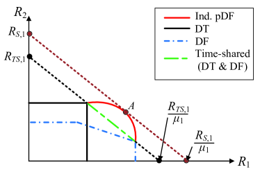
Figure 3: Illustration for comparison between independent pDF relaying and DF-DT time sharing for Regime A in Thm. 2.

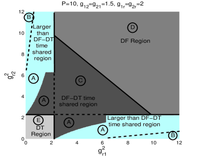
Figure 4: Link-state regions for the independent pDF scheme as specified in Theorem 2.

For the cases where the corner points of the pDF region coincides with the corner points of the DF-DT time-shared region, we examine the maximum weighted sum rate curve of the pDF scheme to see if there is a point outside the DF-DT time-shared region as illustrated in Figure 3. Specifically, we consider an optimization problem of the weighted sum-rate point (point A), where the weights are the same as the coefficients of the slope of the outermost time-sharing line between DF and DT (the dashed green line). The slope coefficient $\mu_{1}$ is obtained based on the easily computed corner points of the DF and DT schemes as shown in (17). We then maximize the weighted sum rate $(R_{2}+\mu_{1}R_{1})$ subject to rate constraints of the pDF scheme. If the maximum weighted sum rate point is outside the DF-DT time-sharing line $(R_{S,1}>R_{TS,1})$, then the pDF scheme strictly outperforms time sharing between DF and DT.

The optimization of the weighted sum rate also reveals the structure of the optimal input signals of the two users. For case A under conditions (11a), this optimization for every given power allocation of user 2’s private message results in the optimal power allocation of user 1’s private message as either $0$ or $P$. Hence, the optimal signal structure for one user is pDF while for the other user is either full DF or DT. The opposite structure holds for conditions (11b).

For case C, we show that full DF scheme maximizes the individual rates of pDF scheme while DT maximizes the sum rate. The rest of the region is obtained by time sharing of DF-DT schemes. For cases D and E, it is easy to show that the optimal power allocations for both private messages are either $0$ or $P$ which reduces the scheme to full DF (case D) or DT (case E).

IV-C Discussion of link regimes

The link regimes of Theorem 2 are graphically illustrated in Figure 4. Denote SNR${}_{ij}=g_{ij}P_{j}$ as the received SNR at use $i$ for signals from node $j$, ignoring any interference or signals from other nodes. The link-state regimes in Theorem 2 can then be expressed in terms of these received SNRs. First, consider regime A under condition (11a) (condition (11b) is similar with the user indices swapped). This condition corresponds to user 1’s relay link slightly stronger than its direct link, SNR${}_{r1}>$SNR₂₁. However, when considering the interference at the relay from user $2$, the received SNR at the relay is less than the received SNR at user $2$ from both user $1$ and the relay, i.e., $\frac{\text{SNR}_{r1}}{1+\text{SNR}_{r2}}<$ $\text{SNR}_{21}+\text{SNR}_{2r}$. Then, the optimal transmission scheme is for user $2$ to perform pDF relaying while user $1$ switches between direct transmission and full DF relaying. The switching transmission from user $1$ depends on the power allocated to the private part of user $2$ as it determines the amount of interference at the relay and hence whether direct transmission or full DF relaying is preferred at user $1$. Performing pDF relaying for user 2 provides two benefits. It allows user 2 the option of achieving its highest individual rate obtained in this case from direct transmission which is a special case of the pDF relaying. But it also allows user $2$ the option of reducing the interference to user 1’s information at the relay since it allows the relay to decode part of user 2’s information, which effectively removes this portion of user 2’s signal from the interference, in order to decode user 1’s information.

In regime B (conditions (13a)), user 1’s relay link is significantly stronger than its direct link such that even when considering the interference at the relay from user $2$, the received SNR at the relay from user $1$ is greater than the received SNR at user $2$ from both user $1$ and the relay, i.e., $\frac{\text{SNR}_{r1}}{1+\text{SNR}_{r2}}>$ $\text{SNR}_{21}+\text{SNR}_{2r}$. Therefore, the hybrid scheme is optimal in this case where user $1$ always performs full DF relaying while user $2$ performs DT. This hybrid scheme gives user 2 its maximum rate in this region while presents no harm to user 1’s rate even under the maximum interference from user $2$ at the relay because of the strong link from user $1$ to relay.

Regime C indicates that when the received SNR at the relay from each user is greater than the received SNR at the other user while the total sum rate at the relay from both users is less than the sum of both DT rates, then the DF-DT time-shared scheme can achieve the same rate region as the pDF scheme. However, in regime D, when the total sum rate at the relay from both users is greater than the sum of both DT rates, then full DF relaying becomes the optimal scheme since both user-to-relay links are strong enough to support full DF relaying. Regime E indicates that when the received SNR at the relay from each user is less than the corresponding direct SNR, the relay should not be used at all, similar to the one-way relay channel.

Independent pDF relaying is rate-optimal in Regimes A, B and C. Under conditions (12) and (14), pDF achieves the same rate region as DF-DT time-sharing; that is, it effectively implements time-sharing in these cases. Under conditions (11) and (13), however, pDF strictly outperforms DF-DT time-sharing.

V A half-duplex decode-forward scheme

In this section, we propose a DF scheme that utilizes coherent relaying, independent relaying and partial relaying for the half-duplex mode. Different from the full-duplex scheme, in the half-duplex mode, each node can only either transmit or receive at each time in the same frequency band. We consider a time-division implementation for the half-duplex mode and propose a $6$-phase scheme as depicted in Figure 1(b).

V-A Transmission scheme

There are several important differences between the half-duplex and full-duplex schemes. First, because of half-duplex transmission, block Markov superposition coding changes to phase superposition coding. In each block, each user transmits only new information and does not repeat old information of the previous block. Each user divides its message into two parts: a private part and a common part, and superposes the private message on the common one. But not all messages are transmitted in each phase. During a specific phase, if only the relay is receiving, then each user transmits only its common message; otherwise, each user transmits both common and private messages. The superposition coding between phases creates a coherent beamforming in certain phases (when a user and the relay both transmit) in a way similar to the full-duplex beamforming created by block Markovity. Second, in each phase, the relay performs only independent coding or coherent coding, but not both. When forwarding both common messages, the relay uses independent coding to send the bin index of this message pair. When forwarding only one common message, the relay uses coherent coding. Third, decoding at each node is performed simultaneuosly across several phases. The relay decodes the common messages at the end of phase $3$, by simultaneously using signals received in all first three phases. Each user decodes the other user’s messages at the end of phase $6$ using all its received signals in its receiving phases. Since user decoding occurs at the end of the same block that information is transmitted, the decoding delay is shorter than in the full-duplex scheme by one block.

Next we describe the signal construction in each phase and decoding rule at each node.

V-A1 Transmit signal construction

Since block index is unnecessary in the half-duplex scheme, we will drop it from the notation. Again let the message of user $i$ be $m_{i}$ for $i\in\{1,2\}$. Each user splits its message as $m_{i}=(m_{i0},m_{ii})$, where $m_{i0}$ is the common message and $m_{ii}$ is the private message. The transmit signals during each phase are as follows:

$$\text{Phase 1:}\quad X_{11} =\sqrt{\alpha_{11}}U_{1}^{(1)}(m_{10})+\sqrt{\beta_{11}}V_{1}^{(1)}(m_{11})$$

$$\text{Phase 2:}\quad X_{22} =\sqrt{\alpha_{22}}U_{2}^{(2)}(m_{20})+\sqrt{\beta_{22}}V_{2}^{(2)}(m_{22})$$

$$\text{Phase 3:}\quad X_{13} =\sqrt{\alpha_{13}}U_{1}^{(3)}(m_{10}),\quad X_{23}=\sqrt{\alpha_{23}}U_{2}^{(3)}(m_{20})$$

$$\text{Phase 4:}\quad X_{14} =\sqrt{\alpha_{14}}U_{1}^{(4)}(m_{10})+\sqrt{\beta_{14}}V_{1}^{(4)}(m_{11}),$$

$$X_{r4} =\sqrt{\gamma_{34}}U_{1}^{(4)}(m_{10})$$

$$\text{Phase 5:}\quad X_{25} =\sqrt{\alpha_{25}}U_{2}^{(5)}(m_{20})+\sqrt{\beta_{25}}V_{2}^{(5)}(m_{22}),$$

$$X_{r5} =\sqrt{\gamma_{35}}U_{2}^{(5)}(m_{20})$$

$$\text{Phase 6:}\quad X_{r6} =\sqrt{{\gamma}_{36}}W(m_{10},m_{20}),$$ (18)

where $U_{i}^{(k)}$ and $V_{i}^{(k)}$ ($i=1,2,k=1\ldots 6$) respectively represent the signal for the common message and the private message of user $i$ in phase $k$, and $W$ represents the signal for the bin index of the common message pair decoded at the relay. All signals $U_{i}^{(k)},V_{i}^{(k)},W$ are independent ${\cal CN}(0,1)$. Note that the signals encode the same information but in different phases are independent of each other (for example, $U_{i}^{(k)}$ all encodes $m_{i0}$ but are independent of each other for different values of $k$); however, the signals encoding the same information in the same phase are fully correlated (for example, in phase 4, user 1 and the relay both send the same signal $U_{1}^{(4)}$ that encodes $m_{10}$, just with different power allocation). Since there is no risk of ambiguity, we will drop phase superscripts in the subsequent discussion.

The power allocation factors $\alpha_{*},\beta_{*},\gamma_{*}$ satisfy the following power constraints:

$$\tau_{1}(\alpha_{11}+\beta_{11})+\tau_{3}\alpha_{13}+\tau_{4}(\alpha_{14}+\beta_{14}) \leq P_{1}$$

$$\tau_{2}(\alpha_{22}+\beta_{22})+\tau_{3}\alpha_{23}+\tau_{5}(\alpha_{25}+\beta_{25}) \leq P_{2},$$

$$\tau_{4}\gamma_{34}+\tau_{5}\gamma_{35}+\tau_{6}{\gamma}_{36} \leq P_{r}.$$ (19)

Note that the above constraints include power control with regards to the phase durations $\tau_{*}$ to ensure that each block has a constant average power.

V-A2 Decoding rules

Again we use ML decoding at each node. The important feature here is that each node uses the received signals in several phases simultaneously. Specifically, the relay is receiving in phases 1, 2 and 3; thus it decodes at the end of phase 3 by using the received signals in all first three phases. Similarly, user 1 decodes at the end of phase 6 by using its received signals in phases $(2,5,6)$; as so does user 2 using received signals in phases $(1,4,6)$.

At the relay, the received signals in the first three phases are

$$Y_{r1} =h_{r1}\sqrt{\alpha_{11}}U_{1}+h_{r1}\sqrt{\beta_{11}}V_{1}+Z_{r1},$$

$$Y_{r2} =h_{r2}\sqrt{\alpha_{22}}U_{2}+h_{r2}\sqrt{\beta_{22}}V_{2}+Z_{r2}$$

$$Y_{r3} =h_{r1}\sqrt{\alpha_{13}}U_{1}+h_{r2}\sqrt{\alpha_{23}}U_{2}+Z_{r3}.$$ (20)

The relay is interested in decoding $(U_{1},U_{2})$ to obtain messages $(m_{10},m_{20})$ and treats $(V_{1},V_{2})$ as noise in this process. The optimal relay decoding rule can be written as follows:

$$\left(m_{10},m_{20}\right)=\arg\max P(U_{1}|Y_{r1})\cdot P(U_{2}|Y_{r2})\cdot P(U_{1},U_{2}|Y_{r3}).$$ (21)

Note here the decoding probability is joint (as a product) across three phases.

Decoding at the users is similar. Since operations at two users are alike, we will only describe the decoding rule for user 2. User 2 is in receiving mode in phases ($1,4,6$) with received signals:

$$Y_{21} =h_{21}\sqrt{\alpha_{11}}U_{1}+h_{21}\sqrt{\beta_{11}}V_{1}+Z_{21},$$

$$Y_{24} =h_{21}\sqrt{\alpha_{14}}U_{1}+h_{21}\sqrt{\beta_{14}}V_{1}+h_{2r}\sqrt{\gamma_{34}}U_{1}+Z_{24}.$$

$$Y_{26} =h_{2r}\sqrt{{\gamma}_{36}}W+Z_{26},$$ (22)

User 2 jointly decodes both messages $(m_{10},m_{11})$ at the end of phase $6$ by the following rule:

$$\left(m_{10},m_{11}\right)=\arg\max P(U_{1},V_{1}|Y_{21})\cdot P(U_{1},V_{1}|Y_{24})$$

$$\;\cdot P(W|Y_{26},m_{20}).$$ (23)

Again the decoding probability is a product across three phases, and in the last phase, the decoding rule utilizes side information of $m_{20}$ available at user 2.

V-B Achievable rate region

With the above transmit signals and decoding rules, we have the following result.

Theorem 3.

The following rate region is achievable for the half-duplex Gaussian two-way relay channel with the above 6-phase partial decode-forward transmission scheme:

$$R_{1} \leq\min\{J_{1}+J_{4},J_{5}\},$$

$$R_{2} \leq\min\{J_{2}+J_{6},J_{7}\},$$

$$R_{1}+R_{2} \leq J_{3}+J_{4}+J_{6},$$ (24)

where

$$J_{1} =\tau_{1}C\left(\frac{g_{r1}^{2}\alpha_{11}}{g_{r1}^{2}\beta_{11}+1}\right)+\tau_{3}C(g_{r1}^{2}\alpha_{13}),$$

$$J_{2} =\tau_{2}C\left(\frac{g_{r2}^{2}\alpha_{22}}{g_{r2}^{2}\beta_{22}+1}\right)+\tau_{3}C(g_{r2}^{2}\alpha_{23})$$

$$J_{3} =\tau_{1}C\left(\frac{g_{r1}^{2}\alpha_{11}}{g_{r1}^{2}\beta_{11}+1}\right)+\tau_{2}C\left(\frac{g_{r2}^{2}\alpha_{22}}{g_{r2}^{2}\beta_{22}+1}\right)$$

$$\;+\tau_{3}C(g_{r1}^{2}\alpha_{13}+g_{r2}^{2}\alpha_{23})$$

$$J_{4} =\tau_{1}C(g_{21}^{2}\beta_{11})+\tau_{4}C(g_{21}^{2}\beta_{14}),$$

$$J_{5} =\tau_{1}C\left(g_{21}^{2}(\alpha_{11}+\beta_{11})\right)+\tau_{6}C(g_{2r}^{2}\gamma_{36})$$

$$\;+\tau_{4}C\left((g_{21}\sqrt{\alpha_{14}}+g_{2r}\sqrt{\gamma_{34}})^{2}+g_{21}^{2}\beta_{14}\right)$$

$$J_{6} =\tau_{2}C(g_{12}^{2}\beta_{22})+\tau_{5}C(g_{12}^{2}\beta_{25})$$

$$J_{7} =\tau_{2}C\left(g_{12}^{2}(\alpha_{22}+\beta_{22})\right)+\tau_{6}C(g_{1r}^{2}\gamma_{36})$$

$$\;+\tau_{5}C\left((g_{12}\sqrt{\alpha_{25}}+g_{1r}\sqrt{\gamma_{35}})^{2}+g_{12}^{2}\beta_{25}\right)$$

and phase duration $\sum_{i}\tau_{i}=1$, power allocation parameters satisfy the constraints in (V-A1).

Proof:

The rate region follows directly from the signal construction and decoding rules in Section V-A. In particular, decoding of common messages at the relay produces rate terms $J_{1},J_{2},J_{3}$ as in a multiple access channel. Decoding of the common and private messages of user 1 at user 2 produces rate terms $J_{4}$ and $J_{5}$ as a direct result of the superposition coding structure. Similarly, $J_{6}$ and $J_{7}$ result from the decoding at user 1. Note that all these rate expressions contain multiple terms that account for the fact that a message is sent, received and decoded simultaneously over multiple phases. ∎

Remark 1.

Employing sequential decoding for the common and then private message parts instead of joint decoding of both message parts can lead to the same achievable rate region. However, simultaneous decoding among the phases must also be employed. Specifically, we can achieve the same rate region as in (3) if user $2$ sequentially decodes the common message part $(m_{10})$ and then the private message part $(m_{11})$ instead of jointly decoding them, provided that user $2$ decodes $m_{10}$ simultaneously from all received signals in phases $1,$ $4$ and $6$ and then decodes $m_{11}$ simultaneously from all received signals in phases $1$ and $4$.

V-C Comparison with existing schemes

In half-duplex rate region (3), by setting the appropriate phase durations to $0$, we can recover existing results. By setting $\tau_{4}=\tau_{5}=0$, the proposed $6$-phase scheme reduces to the 4-phase scheme in our previous work [6], which encompasses the 2, 3 and 4-phase DF schemes in [5].

The proposed scheme is simpler than the 6-phase scheme in [10] as each user splits its message into $2$ parts only instead of $6$ parts as in [10]. In practice, fewer split parts lead to fewer parameters to be optimized for performance. Although sequential decoding used in [10] is simpler than joint decoding, it leads to a smaller achievable rate region. We also show in Remark 1 that sequential decoding can be used to first decode the common and then the private message part provided that the decoding is performed simultaneously among the phases. The rate region of our scheme in Theorem 3 strictly encompasses the rate region of the scheme in [10] by setting $\beta_{11}=\beta_{22}=0$, as also shown in numerical examples in Figure 6.

Our scheme is also simpler in terms of the message splitting than the 6-phase scheme in [7, 8], in which each user splits its message into $3$ parts. However, there is no superposition coding or coherent transmission in this scheme which simplifies its signaling. Specifically, in phases $4$ and $5$, each user and the relay transmit independent signals non-coherently to the other user. The rate region of the scheme in [7, 8] can be obtained from Theorem 3 as a special case by setting $\beta_{11}=\beta_{22}=\alpha_{14}=\alpha_{25}=0$, and is smaller than our achievable rate region.

VI Numerical results

In this section, we provide numerical examples for the rate region achieved by the proposed full and half-duplex schemes and compare it with existing schemes. These regions are obtained by taking the convex closure of all rate regions obtained with all possible resource allocations, including powers and phases [19]. We also provide numerical illustration for the optimal link regimes as shown in Theorem 2. In all figures, we set $P_{1}=P_{2}=P_{r}=P$.

Figures 5 compares between the achievable rate regions in the full-duplex mode for proposed independent and coherent pDF scheme in Theorem 1, existing schemes and the cut-set outer bound under channel conditions specified in the figure. Results show that under such channel conditions, the proposed scheme outperforms all existing schemes and their time-sharing. For the independent pDF scheme, these results are in agreement with Theorem 2. The channel configurations in Figure 5 corresponds to Regime $B$ with condition (13a), under which the composite scheme outperforms time-sharing of existing schemes.

Similar results are obtained for the half-duplex schemes in Figure 6 with link qualities shown on top of the figure. The asymmetric links between the two users can appear in practice in FDD systems. The proposed pDF scheme includes as special cases the $4$-phase schemes in [5][6]. Note that our previous $4$-phase scheme in [6] achieves a rate region very close to that of the $6$-phase composite scheme for the chosen channel configuration. The composite $6$-phase scheme also outperforms the existing $6$-phase schemes [10, 7, 8]. The performance improvement in our scheme comes from the simultaneous decoding among all phases instead of separate decoding at each phase as in [10] or only among a few phases as in [7, 8]. Furthermore, the schemes in [7, 8] do not have coherent relaying.

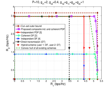
Figure 5: Full-duplex composite pDF scheme achieves rates outside the time-shared region of existing schemes.

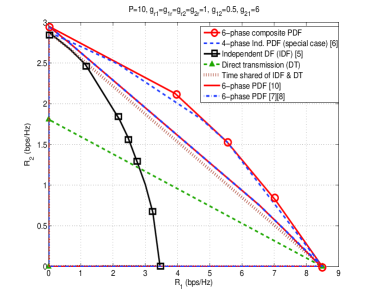
Figure 6: Rate region comparison between the proposed $6$-phase composite and existing schemes in the half-duplex mode.

Figure 7 illustrates the different geometric link regimes on a 2$D$ plane for the independent pDF scheme as described in Theorem 2. The locations of user 1 and user $2$ are fixed at $(-1,0)$ and $(1,0)$, respectively, while the relay can be anywhere on the plane. The path-loss model determines the channel gain between any two nodes based on their relative distance as $g_{ij}=d_{ij}^{-\gamma/2}$ with $\gamma=2.4,$ which is an example for indoor propagation at $900$MHz [21].

The results of Figure 7 match the results and implications of Theorem 2. Figure 7 shows that full DF relaying is optimal when the relay is close to both users and has strong links to them such that it can fully decode their information (case $D$ in Theorem 2). The hybrid scheme with full DF relaying from one user and DT from the other user is optimal when the relay is very close to one user and far from the other (case $B$ in Theorem 2). Switching between full DF relaying and DT from one user and performing pDF from the other user is optimal when the relay is slightly close to one user and far from the other (case $A$ in Theorem 2). Partial DF relaying from both users is optimal when the relay is slightly far from both users, where pDF relaying obtains the same performance as DF-DT time sharing (case $C$ in Theorem 2). DT from both users is optimal when the relay is too far from both users such that decode-and-forward degrades performance (case $E$ in Theorem 2). As the relay moves from afar towards a user, the transmission strategy for that user changes from DT to switching between DF and DT, then to full DF when the relay is very close to that user, and to pDF when the relay is moving further away again. Figure 7 shows that in the regions where the use of relay is viable, independent pDF relaying can improve performance upon existing schemes for a large portion of these regions.

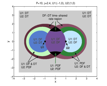
Figure 7: Geometric regions of relay location for the optimal use of different sub-schemes. Some regions overlap when the rate performance is the same.

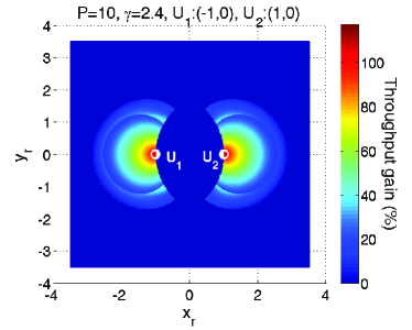
Figure 8: Throughput gain obtained by independent pDF compared with DF-DT time sharing for the same spatial regions in Figure 7.

Figure 8 shows the throughput gain obtained by using the independent pDF scheme compared with the DF-DT time-shared scheme for the same spatial regions as in Figure 7. Specifically, the throughput gain $(\Gamma)$ is obtained as $\Gamma=\frac{R_{S,1}-R_{TS,1}}{R_{TS,1}}100\%$. Results show that in the pDF region in Figure 7 (the black and green regions), independent pDF relaying can improve the throughput by up to $40\%$. Moreover, in the hybrid DF-DT region in Figure 7 (the two blue regions), the hybrid scheme can improve the throughput by more than $100\%$. These gains are significant, especially considering that in the hybrid regions, the optimal strategy is quite simple as having only one user use the relay in the full DF mode while the other performs DT. Even though there is no pDF relaying in the hybrid regions, the knowledge that this hybrid scheme is optimal comes as a direct result of link-regime analysis of pDF relaying. These results emphasize the importance of adapting the transmission schemes according to the link regimes.

VII Conclusion

We have proposed DF-based schemes for the full and half-duplex TWRC that utilize coherent relaying, independent relaying, and partial relaying techniques. The proposed schemes outperforms all existing schemes by achieving a larger rate region. We further analyze independent and partial relaying in detail and analytically derive the link regimes for the optimal use of these techniques. These regimes show when it is necessary to use independent partial DF relaying, and when it is sufficient to use simpler schemes such as full DF relaying or just direct transmission, in order to get the largest possible rate region. Contrast to established results for the one-way relay channel, we show that partial DF relaying can outperform full DF relaying in the TWRC. Independent and partial DF relaying achieves a strictly larger rate region than the DF-DT time-shared region when the relay has strong link with one user and weak link with the other user, or when it has links to both users that are just marginally stronger than their direct links. These link regimes are useful for adapting the proposed schemes to practical link configurations.

Appendix A: Proof of Theorem 1

In this appendix, we provide the proof of Theorem 1 through information theoretic analysis of a discrete memoryless channel specified by a collection of pmf $p(y_{1},y_{2},y_{r}|x_{1},x_{2},x_{r})$, where $x_{k},y_{k}$ ($k=1,2,r$, $r$ stands for the relay) are the input and output signals of node $k$. We define a $(2^{nR_{1}},2^{nR_{2}},n,P_{e})$ code based on standard definitions as in [19].

-1 Codebook generation

The codebook is generated according to the joint distribution

$$P =p(w_{1})p(u_{1}|w_{1})p(x_{1}|u_{1},w_{1})p(w_{2})p(u_{2}|w_{2})$$

$$\;\;\times p(x_{2}|u_{2},w_{2})p(x_{r}|w_{1},w_{2})$$ (25)

The messages of each user are encoded independently by superposition coding. For each block $j\in[1:b]$, according to $p(w_{1})p(u_{1}|w_{1})p(x_{1}|u_{1},w_{1})$, independently generate $2^{nR_{10}}$ codewords $w_{1}^{n}(m_{10,j-1})$, $2^{nR_{10}}$ codewords $(u_{1}^{n}(m_{10,j}|m_{10,j-1}))$ and $2^{nR_{11}}$ codewords $(x_{1}^{n}(m_{11,j}|m_{10,j},m_{10,j-1}))$ that encode $m_{10,j-1},$ $m_{10,j}$ and $m_{11,j}$, respectively. Similarly for user 2’s messages.

The relay only encodes the common messages of both users in the previous block by using both superposition coding and random binning. First, equally and uniformly divide common message pairs $(m_{10},m_{20})$ into $2^{nR_{r}}$ bins and let $K(m_{10},m_{20})$ denote the bin index. Then superpose codewords for bin indices on the codeword generated at each user for each common message. Specifically, for each pair of previous common messages $(m_{10,j-1},m_{20,j-1})$, generate $2^{nR_{r}}$ sequences $x_{r}^{n}(K(m_{10,j-1},m_{20,j-1})|m_{10,j-1},m_{20,j-1})\sim\prod^{n}_{i=1}p(x_{ri}|w_{1i},w_{2i})$.

Decoding at the relay

At the end of block $j$, given $(m_{10,j-1},m_{20,j-1})$ is known, the relay uses joint decoding to find the unique $(\tilde{m}_{10,j},\tilde{m}_{20,j})$ such that

$$(w_{1}^{n},w_{2}^{n},x_{r}^{n},u_{1}^{n}(\tilde{m}_{10,j}|\cdot),u_{2}^{n}(\tilde{m}_{20,j}|\cdot),y^{n}_{r,j})\in T^{(n)}_{\epsilon},$$ (26)

where $\cdot$ denotes known messages and $T^{(n)}_{\epsilon}$ denotes the typical set. As in a multiple access channel, the relay can success with vanishing error as $n\to\infty$ if

$$R_{10} \leq I(U_{1};Y_{r}|W_{1},W_{2},U_{2},U_{r},X_{r})\triangleq I_{1};$$

$$R_{20} \leq I(U_{2};Y_{r}|W_{1},W_{2},U_{1},U_{r},X_{r})\triangleq I_{2};$$

$$R_{10}+R_{20} \leq I(U_{1},U_{2};Y_{r}|W_{1},W_{2},U_{r},X_{r})\triangleq I_{3}.$$ (27)

Decoding at the user

Each user uses forward sliding window decoding over 2 consecutive blocks. Take user 2 for example. Given that it has correctly decoded messages in all blocks up to $j-2$, at the end of block $j$, user 2 finds the unique $(\hat{m}_{10,j-1},\hat{m}_{11,j-1})$ such that

$$\big{(}u_{1}^{n}(\hat{m}_{10,j-1}|\cdot),x_{1}^{n}(\hat{m}_{11,j-1}|\hat{m}_{10,j-1},\cdot),w_{1}^{n},w_{2}^{n},$$

$$x_{r}^{n},u_{2}^{n},x_{2}^{n},y^{n}_{2,j-1}\big{)} \in T^{(n)}_{\epsilon}$$

$$\text{and}\;\;(w_{1}^{n}(\hat{m}_{10,j-1}),x_{r}^{n}(\hat{m}_{10,j-1},\cdot),w_{2}^{n},u_{2}^{n},x_{2}^{n},y^{n}_{2,b}) \in T^{(n)}_{\epsilon}.$$

Following the standard error analysis in [22], we obtain the following rate constraints:

$$R_{11} \leq I(X_{1};Y_{2}|W_{1},U_{1},W_{2},U_{2},X_{2},X_{r})\triangleq I_{4},$$

$$R_{10}+R_{11} \leq I(U_{1},X_{1};Y_{2}|W_{1},W_{2},U_{2},X_{2},X_{r})$$

$$\;\;+I(W_{1},X_{r};Y_{2}|W_{2},U_{2},X_{2})\triangleq I_{5}.$$ (28)

Similarly, for the decoding at user 1 to success with vanishing error,

$$R_{22} \leq I(X_{2};Y_{1}|W_{1},U_{1},W_{2},U_{2},X_{1},X_{r},U_{r})\triangleq I_{6}$$

$$R_{20}+R_{22} \leq I(U_{2},X_{2},W_{2},X_{r},U_{r};Y_{1}|W_{1},U_{1},X_{1})\triangleq I_{7}.$$ (29)

By performing Fourier-Mozkin elimination, we obtain the following achievable rate region:

$$R_{1} \leq\min\{I_{1}+I_{4},I_{5}\},$$

$$R_{2} \leq\min\{I_{2}+I_{6},I_{7}\},$$

$$R_{1}+R_{2} \leq I_{3}+I_{4}+I_{6},$$ (30)

for some joint distribution $P$ as in (25) where $I_{1}$—$I_{7}$ are given in (Decoding at the relay)—(Decoding at the user). Apply the signaling in (3) to Gaussian channel (1), we obtain the rate region in Theorem 1.

Appendix B: Proof of Theorem 2

For the independent pDF scheme, the achievable rate region as in Theorem 1 reduces to that in (Appendix B: Proof of Theorem 2). We will analyze the region in (Appendix B: Proof of Theorem 2) here.

$$R_{1}\leq\min\left\{J_{1},J_{4}\right\},\;\;R_{2}\leq\min\left\{J_{2},J_{5}\right\},$$

$$R_{1}+R_{2}\leq J_{3},\;\;\text{where}$$ (31)

$$J_{1}=C\left(\frac{g_{r1}^{2}{\beta_{1}}}{g_{r1}^{2}\gamma_{1}+g_{r2}^{2}\gamma_{2}+1}\right)+C(g_{21}^{2}\gamma_{1}),$$

$$J_{2}=C\left(\frac{g_{r2}^{2}{\beta_{2}}}{g_{r1}^{2}\gamma_{1}+g_{r2}^{2}\gamma_{2}+1}\right)+C(g_{12}^{2}\gamma_{2}),$$

$$J_{3}=C\left(\frac{g_{r1}^{2}{\beta_{1}}+g_{r2}^{2}{\beta_{2}}}{g_{r1}^{2}\gamma_{1}+g_{r2}^{2}\gamma_{2}+1}\right)+C(g_{21}^{2}\gamma_{1})+C(g_{12}^{2}\gamma_{2}),$$

$$J_{4}=C\left((g_{21}^{2}+g_{2r}^{2})P\right),\;\;J_{5}=C\left((g_{12}^{2}+g_{1r}^{2})P\right),$$

$$0\leq{\beta_{1}},{\beta_{2}}\leq 1,\;\;\beta_{1}+\gamma_{1}=P,\;\;\beta_{2}+\gamma_{2}=P,$$

$$\text{ and }\;\;C(x)=\log(1+x).$$

-A Case $1$: Equations (11) and (12)

We only prove here the conditions in (11a) as those in (11b) can be shown similarly. This case can be divided into the following $4$ subcases:

-A1 Subcase $1.1$: $g_{21}^{2}<g_{r1}^{2}<\min\left\{g_{21}^{2}+g_{2r}^{2}\frac{P_{r}}{P_{1}},\;g_{21}^{2}(1+g_{r2}^{2}P_{2})\right\}$

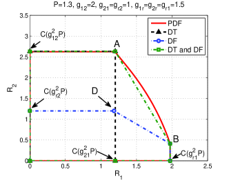
Figure 9: Subcase $1.1$.

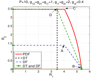
Figure 10: Subcase $1.2$.

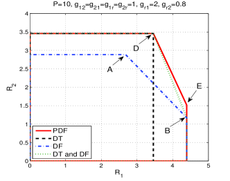
Figure 11: Subcase $1.3$.

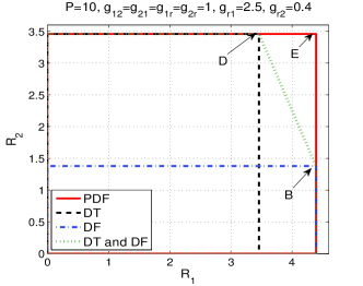
Figure 12: Case $2$.

We only prove here the conditions in (12a) as (12b) can be shown similarly. Figure 9 shows a typical achievable rate regions of the independent pDF, DF and DT schemes for channel parameters that satisfy the conditions in (12a) but with $R_{S1}>R_{TS,1}$.

First, from the conditions $g_{12}^{2}>g_{r2}^{2},$ $g_{r1}^{2}>g_{21}^{2}$ and rate constraints of the DT and DF schemes, we can obtain the coordinates for points $A$ and in $B$ in Figure 9. Then we consider the convex hull of the DF and DT schemes, which is obtained by connecting points $A$ and $B$ with a line that can be formulated as

$$R_{2}+\mu_{1}R_{1} =R_{TS,1},$$

$$\;\;\text{where}\;\mu_{1} \;\text{and}\;R_{TS,1}\;\text{are given in (\ref{ffft})}.$$ (32)

Next, we consider the pDF scheme. It is easy to show that $J_{1}<J_{4}$ since $g_{r1}^{2}>g_{21}^{2}$ and $g_{r1}^{2}<g_{21}^{2}+g_{2r}^{2}\frac{P_{r}}{P_{1}}$ while $J_{2}<J_{5}$ since $g_{12}^{2}>g_{r2}^{2}$. Therefore, the rate region in (Appendix B: Proof of Theorem 2) reduces to

$$R_{1} \leq J_{1},\;\;R_{2}\leq J_{2},\;\;R_{1}+R_{2}\leq J_{3}.$$ (33)

We then maximize $R_{2}+\mu_{1}R_{1}$ in (-A1) for the pDF scheme, subject to rate constraints in (33), and compare the results with $R_{TS,1}$.

Based the channel conditions for this subcase and by considering points $A$ and $D$ in Figure 9, we have $R_{1}(A)>R_{1}(D)$ and $R_{2}(A)>R_{2}(D)$. Hence, the slope of the time sharing line (between $A$ and $B$) is greater than the slope of the full DF scheme (between $D$ and $B$), leading to $\mu>1$. Furthermore, the achievable rate for the pDF scheme in (33) is a pentagon for any fixed power allocation where the line connecting the upper and lower corner points has a slope of $1$. Therefore, we only need to maximize the lower corner point (point $C$) of this pentagon, i.e. $(R_{1}(C),R_{2}(C))=(J_{1},J_{3}-J_{1})$. If this point is inside the time shared region, the upper corner point will also be inside the time shared region.

By substituting $\beta_{1}=P_{1}-\gamma_{1}$ and $\beta_{2}=P_{2}-\gamma_{2}$ into the lower corner point $(R_{1}(C),R_{2}(C))=(J_{1},J_{3}-J_{1})$, we obtain the following problem to maximize $R_{2}+\mu_{1}R_{1}$:

$$\max_{\begin{subarray}{c}\gamma_{1},\gamma_{2}\end{subarray}}f(\gamma_{1},\gamma_{2}) ,\quad\text{where}$$ (34)

$$f(\gamma_{1},\gamma_{2}) =J_{3}-J_{1}+\mu_{1}J_{1},$$

$$\Rightarrow f(\gamma_{1},\gamma_{2}) =C\left(g_{r1}^{2}P_{1}+g_{r2}^{2}P_{2}\right)-C\left(\frac{g_{r1}^{2}P_{1}}{1+g_{12}^{2}\gamma_{2}}\right)$$

$$\;-\mu_{1}\left(C\left(\frac{g_{r1}^{2}{\beta_{1}}}{g_{r1}^{2}\gamma_{1}+g_{r2}^{2}\gamma_{2}+1}\right)+C(g_{21}^{2}\gamma_{1})\right),$$

and $J_{1}$ and $J_{3}$ are as given in (Appendix B: Proof of Theorem 2). We decompose this problem into $2$ steps where we find the optimal $\gamma_{1}^{\ast}$ for a fixed $\gamma_{2}$ and then find the optimal $\gamma_{2}^{\ast}$. We find that $f(\gamma_{1},\gamma_{2})$ is either monotonically increasing or decreasing in $\gamma_{1}$ depending on the value of $\gamma_{2}$ since $\frac{\partial f(\gamma_{1},\gamma_{2})}{\partial\gamma_{1}}\gtrless 0\;\Leftrightarrow\;\gamma_{2}\gtrless\frac{g_{r1}^{2}-g_{21}^{2}}{g_{21}^{2}g_{r2}^{2}}.$ Hence, for any value of $\gamma_{2},$ the optimal $\gamma_{1}^{\ast}$ is either $0$ or $P$. By setting $\gamma_{1}^{\ast}=P$, we find that $\gamma_{2}^{\ast}=P$ since $\frac{\partial f(\gamma_{1},\gamma_{2})}{\partial\gamma_{2}}>0$ under condition $g_{12}^{2}>g_{r2}^{2}$. At $\gamma_{1}^{\ast}=\gamma_{2}^{\ast}=P$, we obtain the point $A$ in Figure (9) which is the same for both the pDF scheme and the DF-DT time shared scheme. Hence, at this point, $R_{2}+\mu_{1}R_{1}=R_{TS,1}$. On the other hand, when $\gamma_{1}^{\ast}=0$, we obtain $\gamma_{2}^{\ast}$ in (17) by setting $\frac{\partial f(\gamma_{1},\gamma_{2})}{\partial\gamma_{2}}=0$. If $\gamma_{2}^{\ast}$ in (17) is negative, then $\frac{\partial f(\gamma_{1},\gamma_{2})}{\partial\gamma_{2}}<0$ for $\gamma_{2}\in[0,P]$ and $f(0,\gamma_{2})$ is a decreasing function of $\gamma_{2}$ which makes $\gamma_{2}^{\ast}=0$. Therefore, $\gamma_{2}^{\ast}$ is given as in (17). After that, we have $R_{2}+\mu_{1}R_{1}=f(0,\gamma_{2}^{\ast})$. Hence, to compare with the time-shared scheme, we only need to compare the point at $(\gamma_{1},\gamma_{2})=(0,\gamma_{2}^{\ast})$.

Specifically, we compare $f(0,\gamma_{2}^{\ast})$ with $R_{TS,1}$. If $f(0,\gamma_{2}^{\ast})>R_{TS,1}$, then pDF achieves a larger rate region than the DF-DT time shared region, which corresponds to (13a) where $f(0,\gamma_{2}^{\ast})=R_{S,1}$ in (17). If $f(0,\gamma_{2}^{\ast})<R_{TS,1}$, then pDF achieves the same region as the DF-DT time shared region (condition (12a)). Last, the curve connecting the points $A$ and $B$ is obtained by varying $\gamma_{2}\in[0,P]$ while keeping $\gamma_{1}^{\star}=0$. Hence the optimal scheme always have user 1 performing full DF, while user 2 performing partial DF.

-A2 Subcase $1.2$: $g_{21}^{2}(1+g_{r2}^{2}P_{2})<g_{r1}^{2}<g_{21}^{2}+g_{2r}^{2}\frac{P_{2}}{P_{1}}$

Figure 10 illustrates a typical example for this subcase. It can be proved by following a similar procedure to case $1.1$ except that we need to consider the time shared region of the DF scheme and the hybrid scheme (user 1: DF, user $2$: DT). The convex hull of this time shared region is obtained by connecting points C and B with a line as in case $1.1,$ where the coordinates of point B is $(R_{1}(B),R_{2}(B))=(C(g_{r1}^{2}P_{1}),C(\frac{g_{r2}^{2}P_{2}}{1+g_{r1}^{2}P_{1}}))$ and for point C is $(R_{1}(C),R_{2}(C))=(C(\frac{g_{r1}^{2}P_{1}}{1+g_{r2}^{2}P_{2}}),C(g_{12}^{2}P_{2}))$.

-A3 Subcase $1.3$: $g_{21}^{2}+g_{2r}^{2}\frac{P_{r}}{P_{1}}<g_{r1}^{2}<g_{21}^{2}(1+g_{r2}^{2}P_{2})$

Figure 11 illustrates a typical example for this case. We show here that pDF can achieve point $E$ which is outside the DF-DT time-shared region. Staring with the full DF scheme $(\gamma_{1}=\gamma_{2}=0)$, the rate region in (Appendix B: Proof of Theorem 2) becomes

$$R_{1} \overset{(a)}{\leq}C(g_{21}^{2}P_{1}+g_{2r}^{2}P_{r}),\;\;R_{2}\overset{(b)}{\leq}C(g_{r2}^{2}P_{2}),$$

$$R_{1}+R_{2} \leq C(g_{r1}^{2}P_{1}+g_{r2}^{2}P_{2}),$$ (35)

where $(a)$ follows since $g_{r1}^{2}>g_{21}^{2}+g_{2r}^{2}\frac{P_{r}}{P_{1}}$ while $(b)$ follows since $g_{12}^{2}>g_{r2}^{2}$. Then, the coordinates of point $B$ in Figure 11 are $R_{1}(B)=C(g_{21}^{2}P_{1}+g_{2r}^{2}P_{r})$ and $R_{2}(B)=C(g_{r1}^{2}P_{1}+g_{r2}^{2}P_{2})-C(g_{21}^{2}P_{1}+g_{2r}^{2}P_{r})$.

Now consider the pDF scheme and its achievable region in (Appendix B: Proof of Theorem 2). At $R_{2}=0$ $(\gamma_{2}=\beta_{2}=0)$, $R_{1}^{\max}=C(g_{21}^{2}P_{1}+g_{2r}^{2}P_{r})$ since $J_{1}(\gamma_{1})$ in (Appendix B: Proof of Theorem 2) is a decreasing function of $\gamma_{1}$ and $J_{1}(0)=C(g_{r1}^{2}P_{1})>C(g_{21}^{2}P_{1}+g_{2r}^{2}P_{r})$. Therefore, $R_{1}$ is the same for points $B$ and $E$ $(R_{1}(E)=R_{1}(B))$.

Next, we need to find $R_{2}^{\max}$ such that $R_{1}=C(g_{21}^{2}P_{1}+g_{2r}^{2}P_{r})$. More specifically, we need to find $\gamma_{2}^{\max}$ such that $J_{1}\geq J_{4}$. Consider $\gamma_{1}=0$, we have

$$J_{1}\geq J_{4}\Leftrightarrow\log\left(1+\frac{g_{r1}^{2}P_{1}}{1+g_{r2}^{2}\gamma_{2}}\right)\geq\log(1+g_{21}^{2}P_{1}+g_{2r}^{2}P_{r})$$

$$\Leftrightarrow\gamma_{2}\leq\frac{1}{g_{r2}^{2}}\left(\frac{g_{r1}^{2}}{g_{21}^{2}+g_{2r}^{2}\frac{P_{r}}{P_{1}}}-1\right)=\gamma_{2}^{\max}.$$

With this value of $\gamma_{2}$, $J_{1}(\gamma_{1})$ is a decreasing function of $\gamma_{1}$ since $\frac{\partial J_{1}}{\partial\gamma_{1}}<0$. Hence, setting $\gamma_{1}=0$ is in fact optimal. Note that since $\gamma_{2}\leq P_{2}$, $\gamma_{2}^{\max}$ is given as follows:

$$\gamma_{2}^{\max}=$$ (36)

$$\left\{\begin{array}[]{cl}\frac{1}{g_{r2}^{2}}\left(\frac{g_{r1}^{2}}{g_{21}^{2}+g_{2r}^{2}\frac{P_{r}}{P_{1}}}-1\right)&\text{if}\;\;g_{r1}^{2}<\left(g_{21}^{2}+g_{2r}^{2}\frac{P_{r}}{P_{1}}\right)(1+g_{r2}^{2}P_{2})\\ P_{2},&\text{if}\;\;g_{r1}^{2}\geq\left(g_{21}^{2}+g_{2r}^{2}\frac{P_{r}}{P_{1}}\right)(1+g_{r2}^{2}P_{2})\end{array}\right.$$ (39)

However, since $g_{r1}^{2}<g_{21}^{2}(1+g_{r2}^{2}P_{2})$ for this case, we have $\gamma_{2}^{\max}=\frac{1}{g_{r2}^{2}}\left(\frac{g_{r1}^{2}}{g_{21}^{2}+g_{2r}^{2}\frac{P_{r}}{P_{1}}}-1\right)$. After that, define $J_{i}(\gamma_{1},\gamma_{2})$ for $i\in\{1:5\}$ as $J_{i}$ in (Appendix B: Proof of Theorem 2) obtained with $\gamma_{1}$ and $\gamma_{2}$. Then, with $\gamma_{1}=0$ and $\gamma_{2}=\gamma_{2}^{\max}$, the achievable rate region in (Appendix B: Proof of Theorem 2) is given as

$$R_{1} \leq C(g_{21}^{2}P_{1}+g_{2r}^{2}P_{r}),\;\;R_{2}\leq J_{2}(0,\gamma_{2}^{\max}),$$

$$R_{1}+R_{2} \leq J_{3}(0,\gamma_{2}^{\max}).$$ (40)

Then, $J_{3}(0,\gamma_{2}^{\max})<C(g_{21}^{2}P_{1}+g_{2r}^{2}P_{r})+J_{2}(0,\gamma_{2}^{\max})$ since

$$J_{3}(0,\gamma_{2}^{\max})-J_{2}(0,\gamma_{2}^{\max})$$

$$=C\left(\frac{g_{r1}^{2}P_{1}}{g_{r2}^{2}P_{2}+1}\right)\overset{(a)}{<}C(g_{21}^{2}P_{1}+g_{2r}^{2}P_{r}).$$

where $(a)$ follows from (36). Hence, in Figure 11, $R_{2}(E)=J_{3}(0,\gamma_{2}^{\max})-C(g_{21}^{2}P_{1}+g_{2r}^{2}P_{r})>R_{2}(B)$ since $R_{2}(E)-R_{2}(B)=C(g_{12}^{2}\gamma_{2}^{\max})-C(g_{r2}^{2}\gamma_{2}^{\max})>0.$ Then, point $E$ is outside the DF-DT time-shared region. To show switching between DF and DT is optimal for user $1$, follow the same proof in subcase $1.1$.

-A4 Subcase $1.4$: $\max\left\{g_{21}^{2}+g_{2r}^{2}\frac{P_{r}}{P_{1}},\;g_{21}^{2}(1+g_{r2}^{2}P_{2})\right\}<g_{r1}^{2}<\left(g_{21}^{2}+g_{2r}^{2}\frac{P_{r}}{P_{1}}\right)(1+g_{r2}^{2}P_{2})$

This case includes both subcases $1.2$ and $1.3$ and has a similar proof to these cases.

-B Case $2$: conditions (13)

This case can be simply proved by considering $\gamma_{2}^{\max}$ in (36) for subcase $1.3$. If $g_{r1}^{2}\geq\left(g_{21}^{2}+g_{2r}^{2}\frac{P_{r}}{P_{1}}\right)(1+g_{r2}^{2}P_{2})$, then $\gamma_{2}=P_{2}$ and $\gamma_{1}=0$ which locates point $E$ in the upper corner as shown in Figure 12. Then, point $E$ is also outside the DF-DT time-shared region. Point $E$ and $C$ collide and they are achieved by user $1$ doing full DF and user $2$ doing DT. Since the rate region for this case is a rectangle as shown in Figure 12, DF from user $1$ and DT from user $2$ are optimal to achieve the full rate region.

-C Case $3$: conditions (14)

The conditions for this case are given in (14). Note that the third condition is equivalent to $C(g_{r1}^{2}P_{1}+g_{r2}^{2}P_{2})<C(g_{21}^{2}P_{1})+C(g_{12}^{2}P_{2})$. Considering the rate region in (Appendix B: Proof of Theorem 2), it easy to show that setting $\gamma_{1}^{\ast}=\gamma_{2}^{\ast}=0$ maximizes the individual rates of this region while setting $\gamma_{1}^{\ast}=P_{1}$ and $\gamma_{2}^{\ast}=P_{2}$ maximizes the sum rate of this region. By taking the convex closure of the two regions resulting from these two settings, we obtain the time shared region of the DF and DT schemes.

-D Case 4 and 5: conditions (15) and (16)

Considering rate region (Appendix B: Proof of Theorem 2) with the conditions in (15) (reps. (16)), we maximize the rate region by setting $\gamma_{1}^{\ast}=\gamma_{2}^{\ast}=0$ (resp. $\gamma_{1}^{\ast}=P_{1},\;\gamma_{2}^{\ast}=P_{2}$). Hence, the pDF scheme reduces to DF (resp. DT) scheme.

References

- [1] L. Lei, Z. Zhnog, C. Lin, and X. Shen, “Operator controlled device-to-device communications in LTE-advanced networks,” IEEE Wireless Commun., vol. 19, no. 3, pp. 96–104, Jun. 2012.
- [2] B. Rankov and A. Wittneben, “Achievable rate regions for the two-way relay channel,” in IEEE Int’l Symp. on Info. Theory (ISIT), 2006, pp. 1668–1672.
- [3] L. Xie, “Network coding and random binning for multi-user channels,” in IEEE 10th Canadian Workshop on Info. Theory (CWIT), pp. 85–88.
- [4] P. Zhong and M. Vu, “Decode-forward and compute-forward coding schemes for the two-way relay channel,” in IEEE Information Theory Workshop (ITW), Oct. 2011, pp. 115–119.
- [5] S. Kim, P. Mitran, and V. Tarokh, “Performance bounds for bidirectional coded cooperation protocols,” IEEE Trans. on Info. Theory, vol. 54, no. 11, pp. 5235–5241, Nov. 2008.
- [6] P. Zhong and M. Vu, “Partial decode-forward coding schemes for the gaussian two-way relay channel,” in IEEE Int’l Conference on Commu. (ICC), June 2012, pp. 2451–2456.
- [7] K. Ishaque Ashar, V. Prathyusha, S. Bhashyam, and A. Thangaraj, “Outer bounds for the capacity region of a gaussian two-way relay channel,” in 50th Annual Allerton Conf. on Comm., Control, and Computing, Oct. 2012, pp. 1645–1652.
- [8] C. Gong, G. Yue, and X. Wang, “A transmission protocol for a cognitive bidirectional shared relay system,” IEEE J. Sel. Top. Sign. Proces., vol. 5, no. 1, pp. 160–170, Feb. 2011.
- [9] M. Khafagy, A. El-Keyi, M. Nafie, and T. ElBatt, “Degrees of freedom for separated and non-separated half-duplex cellular mimo two-way relay channels,” in IEEE Int’l Conference on Commu. (ICC), Jun. 2012, pp. 2445–2450.
- [10] L. Gerdes, M. Riemensberger, and W. Utschick, “Bounds on the capacity regions of half-duplex gaussian mimo relay channels,” EURASIP Journal on Advances in Signal Processing, Special Issue on Advanced Distributed Wireless Communication Techniques Theory and Practice, 2013.
- [11] T. Cover and A. El Gamal, “Capacity theorems for the relay channel,” IEEE Trans. on Info. Theory, vol. 25, no. 5, pp. 572–584, 1979.
- [12] C. Schnurr, S. Stanczak, and T. Oechtering, “Achievable rates for the restricted half-duplex two-way relay channel under a partial-decode-and-forward protocol,” in IEEE Information Theory Workshop (ITW), May 2008, pp. 134–138.
- [13] A. El Gamal, M. Mohseni, and S. Zahedi, “Bounds on capacity and minimum energy-per-bit for AWGN relay channels,” IEEE Trans. on Info. Theory, vol. 52, no. 4, pp. 1545–1561, Apr. 2006.
- [14] Z. Chen, H. Liu, and W. Wang, “On the optimization of decode-andforward schemes for two-way asymmetric relaying,” in IEEE Int’l Conference on Commu. (ICC), Jun. 2011, pp. 1–5.
- [15] Y. Shim and H. Park, “A closed-form expression of optimal time for two-way relay using DF MABC protocol,” IEEE Communications Letters, vol. PP, no. 99, pp. 1–4, 2014.
- [16] K. Jitvanichphaibool, R. Zhang, and Y.-C. Liang, “Optimal resource allocation for two-way relay-assisted OFDMA,” IEEE Trans. Veh. Technol., vol. 58, no. 7, pp. 3311–3321, Sept. 2009.
- [17] F. He, Y. Sun, L. Xiao, X. Chen, C.-Y. Chi, and S. Zhou, “Optimal resource allocation for two-way relay-assisted OFDMA,” IEEE Trans. Wireless Commun., vol. 12, no. 6, pp. 2904–2917, Jun. 2013.
- [18] L. Pinals and M. Vu, “Link-state optimized decode-forward transmission for two-way relaying,” submitted to IEEE Trans. on Commu., Jan. 2015.
- [19] A. El Gamal and Y.-H. Kim, Network Information Theory. Cambridge University Press, 2011.
- [20] L. Pinals and M. Vu, “Link state based decode-forward schemes for two-way relaying,” in International Workshop on Emerging Technologies for 5G Wireless Cellular Networks, IEEE Globecom, Dec. 2014.
- [21] T. S. Rappaport, Wireless Communications: Principles and Practice, 2nd ed. Prentice Hall, 2002.
- [22] R. El Gamal and Y.-H. Kim, Network Information Theory, 1st ed. Cambridge University Press, 2011.