LIMITS AND FITS FROM SIMPLIFIED MODELS 

Abstract

An important tool for interpreting LHC searches for new physics are simplified models. They are characterized by a small number of parameters and thus often rely on a simplified description of particle production and decay dynamics. We compare the interpretation of current LHC searches for hadronic jets plus missing energy signatures within simplified models with the interpretation within complete supersymmetric and same-spin models of quark partners. We found that the differences between the mass limits derived from a simplified model and from the complete models are moderate given the current LHC sensitivity. We conclude that simplified models provide a reliable tool to interpret the current hadronic jets plus missing energy searches at the LHC in a more model-independent way.

1 Introduction

In order to cover a broad part of BSM theories’ parameter space, current searches for new physics at the LHC use simplified models motivated by supersymmetry to quantify their results [1, 2, 3, 4, 5]. Several recently developed tools [6, 7, 8, 9] use simplified model results to enable one to test BSM theories against LHC results. It is thereby assumed that upper limits calculated from signal efficiencies for simplified models are mostly unchanged compared to more realistic, more complicated models that include more particles or even have particles with a different spin.

One simplified SUSY model for squarks called T2, shown in figure 2, includes light-flavor squarks, where squarks decay to a quark and a lightest supersymmetric stable particle (LSP). Gluinos (as all other supersymmetric particles except the LSP) are decoupled, and it is assumed that the quark partners produced in this simplified model are scalar particles.

We investigated the effects of adding a finite-mass gluino to the simplified model of squarks used by the experimental collaborations, as well as the influence on mass limits upon changing the spin assumption.

2 Production of squarks at the LHC

In the simplified model of squark production T2, since only light-flavor squarks are present, the blob in figure 2 is represented by the diagrams for squark-antisquark production shown in figure 3. Squark-antisquark production occurs also through the exchange of a gluino in the $t$-channel when a finite-mass gluino is present, as shown in figure 2. With the presence of this diagram, squark pair production and mixtures of left- and right-handed squark production occur as well. That is, instead of only ${\widetilde{q}}_{\mathrm{L}}{\widetilde{q}}_{\mathrm{L}}^{*}$ production, in the case of finite $m_{\widetilde{g}}$ we also have ${\widetilde{q}}_{\mathrm{L}}{\widetilde{q}}_{\mathrm{L}}$, ${\widetilde{q}}_{\mathrm{L}}{\widetilde{q}}_{\mathrm{R}}$ and ${\widetilde{q}}_{\mathrm{L}}{\widetilde{q}}_{\mathrm{R}}^{*}$ production (as well as ${\mathrm{R}}\leftrightarrow{\mathrm{L}}$, with equal cross sections for mass-degenerate squarks).

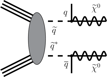
Figure 1: The simplified model T2 for squark production at the LHC as used by the experimental collaborations. The gluino is decoupled.

Figure 2: The $t$-channel gluino diagrams that contribute only when finite-mass gluinos are present.

=   $\Bigg{\{}$ $\Bigg{\}}$

Figure 3: The diagrams contributing to squark-antisquark production in the T2 supersymmetric simplified model.

3 Limits for MSSM-like squarks and LSPs

Adding a finite-mass gluino to the simplified model T2, we obtain what we named MSSM-like squark production. To investigate the differences in limits obtained from efficiencies of this model versus limits from efficiencies for the T2 model in the ${m_{\tilde{q}}}$-$m_{\tilde{\chi}^{0}_{1}}$ mass plane, we used two strongly excluding [6, 9, 10] SUSY analyses CMS-SUS-13-012 [11] and CMS-SUS-12-028 [12], which we named according to their main cut variables MHT and $\alpha_{T}$, respectively.

Using a simulation of the 8 TeV LHC with MadGraph 5 [13], Pythia 6 [14], and Delphes 3 [15, 16] and our own implementations of the MHT and $\alpha_{T}$ analyses, we obtained efficiencies from which we calculated upper limits with RooStatS [21]. Upon comparing these upper limits with the NLO prediction for the cross section of the MSSM-like squark production that was calculated with Prospino [17], we obtained the red solid lines in figure 4 [18].

Figure 4: 95% C.L. exclusion limits at the 8 TeV LHC derived from the full finite-mass gluino $\mathrm{T2}_{m_{\tilde{g}}}$ model (red solid curves) and from the efficiencies for the T2, or $\mathrm{T2}_{\infty}$ simplified model (blue dashed curves). The shaded regions around the curves denote the uncertainties due to scale variation ($\mu={m_{\tilde{q}}}/2,2{m_{\tilde{q}}}$).

Repeating the process for calculating limits from efficiencies for the T2 model, and again comparing with the NLO prediction for the cross section of the MSSM-like squark production, we obtained the blue dashed lines in figure figure 4. The blue and red exclusion lines are within the error for the theoretical prediction of the cross section of the full model exclusions.

Note that the limits shown are from our own simulations and for the most sensitive bin only that was calculated with a pure background hypothesis. CMS, on the contrary, combines bins; this procedure can be expected to yield stronger exclusion limits.

4 Production of same-spin quark partners at the LHC

When one assumes that in the T2 model same-spin instead of scalar quark partners are produced, the exclusion limits from the original scalar quark partner T2 model may change. In this case of same-spin KK quark production, the blob in figure 2 is for UED-like quark production represented by the three diagrams shown in figure 5.

=   $\Bigg{\{}$ $\Bigg{\}}$

Figure 5: The diagrams contributing to KK quark pair production for the UED equivalent of the T2 simplified model. D stands for doublet, as $q_{\mathrm{D}}$ is an SU(2) doublet quark.

As before for MSSM-like squark production, when the gluon partner mass is finite, an additional $t$-channel diagram appears, yielding not only KK quark-antiquark production $q_{\mathrm{D}}\bar{q}_{\mathrm{D}}$ (where D, S stand for SU(2) doublet and singlet, respectively), but also KK quark pair and mixed doublet and singlet production $q_{\mathrm{D}}q_{\mathrm{D}}$, $q_{\mathrm{D}}q_{\mathrm{S}}$ and $q_{\mathrm{D}}\bar{q}_{\mathrm{S}}$ (and $\mathrm{D}\leftrightarrow\mathrm{S}$ with equal cross sections).

5 Limits for UED-like quarks and LKPs

We investigated the difference in limits obtained for a model of UED-like quark production from the full model, containing spin-1/2 quark partners and a finite gluon partner mass, as opposed to limits for this model from the SUSY-T2 model containing scalar quark partners and no gluon partner. Following the same procedure as described in the previous section, with now MadGraph 5 LO cross section predictions of UED-like quark production, we again find that the limit curves in the quark partner and LKP mass plane are close [19], as shown in figure 6. The $\alpha_{T}$ analysis slightly underestimates, whereas the MHT analysis overestimates the limits.

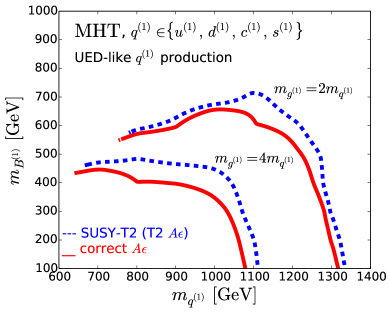
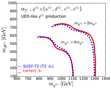
Figure 6: Limits for a model of UED-like quark production at the 8 TeV LHC from the simplified SUSY-T2 model (blue dashed line) and from a simulation of the full model (red solid line). Same-spin quark partners are denoted $q^{(1)}$; the lightest KK particle is denoted $B^{(1)}$.

Note that for this model, the limits are up to 1300 GeV quark partner masses. Most experimental results up to now, however, present limits up to 1 TeV squark masses. This means that when a BSM model with higher cross sections than a simplified SUSY model is tested against those results, a tool like SModelS would not contain and hence not yield any results in these higher mass regions.

6 Conclusion

We conclude that simplified models are a good approximation for (1) more general models of supersymmetry and (2) same-spin models that are not originally described by these models [18, 19].

Since recasting simplified model results is faster than a complete analysis of a specific model or calculating efficiencies for that model, they are ideal for performing global fits using e.g. a combination of SModelS [6, 9] and Fittino [20].

References

References

- [1] N. Arkani-Hamed et al., hep-ph/0703088 [HEP-PH].
- [2] J. Alwall, P. Schuster and N. Toro, Phys. Rev. D 79, 075020 (2009) [arXiv:0810.3921 [hep-ph]].
- [3] D. Alves et al. [LHC New Physics Working Group], J. Phys. G 39, 105005 (2012) [arXiv:1105.2838 [hep-ph]].
- [4] D. S. M. Alves, E. Izaguirre and J. G. Wacker, JHEP 1110, 012 (2011) [arXiv:1102.5338 [hep-ph]].
- [5] S. Chatrchyan et al. [CMS Collaboration], Phys. Rev. D 88, no. 5, 052017 (2013) [arXiv:1301.2175 [hep-ex]].
- [6] S. Kraml et al., Eur. Phys. J. C 74, 2868 (2014) [arXiv:1312.4175 [hep-ph]].
- [7] M. Drees et al., Comput. Phys. Commun. 187, 227 (2014) [arXiv:1312.2591 [hep-ph]].
- [8] M. Papucci, K. Sakurai, A. Weiler and L. Zeune, Eur. Phys. J. C 74, no. 11, 3163 (2014) [arXiv:1402.0492 [hep-ph]].
- [9] S. Kraml et al., arXiv:1412.1745 [hep-ph].
- [10] W. Beenakker, R. Hopker, M. Spira and P. M. Zerwas, Nucl. Phys. B 492, 51 (1997) [hep-ph/9610490].
- [11] S. Chatrchyan et al. [CMS Collaboration], JHEP 1406, 055 (2014) [arXiv:1402.4770 [hep-ex]].
- [12] S. Chatrchyan et al. [CMS Collaboration], Eur. Phys. J. C 73, no. 9, 2568 (2013) [arXiv:1303.2985 [hep-ex]].
- [13] J. Alwall et al., JHEP 1407, 079 (2014) [arXiv:1405.0301 [hep-ph]].
- [14] T. Sjostrand, S. Mrenna and P. Z. Skands, JHEP 0605, 026 (2006) [hep-ph/0603175].
- [15] J. de Favereau et al., JHEP 1402, 057 (2014) [arXiv:1307.6346 [hep-ex]].
- [16] M. Cacciari, G. P. Salam and G. Soyez, Eur. Phys. J. C 72, 1896 (2012) [arXiv:1111.6097 [hep-ph]].
- [17] W. Beenakker, R. Hopker and M. Spira, hep-ph/9611232.
- [18] L. Edelhäuser, J. Heisig, M. Krämer, L. Oymanns and J. Sonneveld, JHEP 1412, 022 (2014) [arXiv:1410.0965 [hep-ph]].
- [19] L. Edelhäuser, M. Krämer and J. Sonneveld, JHEP 1504 146 (2015) [arXiv:1501.03942 [hep-ph]].
- [20] P. Bechtle et al., PoS EPS -HEP2013, 313 (2013) [arXiv:1310.3045 [hep-ph]].
- [21] G. Schott for the RooStats Team, (2012) [arXiv:1203.1547 [physics.data-an]].