Warm intermediate inflation in the Randall-Sundrum II model in the light of Planck 2015 and BICEP2 results: A general dissipative coefficient

Abstract

A warm inflationary Universe in the Randall-Sundrum II model during intermediate inflation is studied. For this purpose, we consider a general form for the dissipative coefficient $\Gamma(T,\phi)=C_{\phi}\,\frac{T^{m}}{\phi^{m-1}}$, and also analyze this inflationary model in the weak and strong dissipative regimes. We study the evolution of the Universe under the slow-roll approximation and find solutions to the full effective Friedmann equation in the brane-world framework. In order to constrain the parameters in our model, we consider the recent data from the BICEP2-Planck 2015 data together with the necessary condition for warm inflation $T>H$, and also the condition from the weak (or strong) dissipative regime.

I Introduction

In modern cosmology, our notions concerning the physics of the very early Universe have introduced a new element, the inflationary period R1 ; R102 ; R103 ; R104 ; R105 ; R106 , which provides an attractive approach for solving some problems of the standard Big-Bang model, like the flatness, horizon, monopoles, among other. However, the essential feature of inflation is that can generate a novel mechanism to explain the Large-Scale Structure (LSS) of the Universe R2 ; R202 ; R203 ; R204 ; R205 and provide a causal interpretation of the origin of the anisotropies observed in the Cosmic Microwave Background (CMB) radiationastro ; astro2 ; astro202 ; Hinshaw:2012aka ; Ade:2013zuv ; Ade:2013uln ; Planck2015 .

By other hand, with respect to the dynamical mechanisms of inflation, the warm inflation scenario, as opposed to the standard cold inflation, has the attractive feature that it avoids the reheating period at the end of the accelerated expansion, because of the decay of the inflaton field into radiation and particles during the slow-roll phase warm . During the warm inflation scenario the dissipative effects are important, since radiation production occurs concurrently together with the inflationary expansion. The dissipating effects arise from a friction term which describes the process of the scalar field decaying into a thermal bath. Also, during the scenario of warm inflation the thermal fluctuations arises from the inflationary epoch may play a fundamental function in producing the initial fluctuations indispensable for the Large-Scale Structure (LSS) formation 62526 ; 1126 . An indispensable condition for warm inflation scenario to occur is the presence of a radiation field with temperature $T>H$ during the inflationary expansion of the Universe. Since the thermal and quantum fluctuations are proportional to $T$ and $H$, respectively warm ; 62526 ; 1126 , so when $T>H$, the thermal fluctuations of the inflaton field predominates over the quantum fluctuations. Also, inflation ends when the Universe heats up to become radiation dominated, and then the Universe smoothly enters to the radiation dominated era, without the need of a reheating scenario warm . For a review of warm inflation, see e.g. Ref. Berera:2008ar .

On the other hand, cosmological implications of string/M-theory have currently attracted a great deal of attention; specifically some were concerned with brane-antibrane configurations such as space-like branes sen1 . In this configuration, the standard model of particles is confined to the brane, while gravitation propagates into the bulk space-time. Here, the effect of extra dimensions induces extra terms in the Friedmann equation 1 ; 3 ; 8 . In particular, the cosmological Randall-Sundrum II model (RS II) has received great attention in the last yearsRS . Randall and Sundrum suggested two similar but phenomenologically different brane world scenarios. In this form, there are two versions of the Randall-Sundrum model, generally mentioned as Randall-Sundrum I (RS1)RS1 and Randall-Sundrum II (RS2)RS . Somewhat confusingly, the RS1 model includes two branes, while the RS2 model only contains a single brane.

In the RS1 model, we have two 3-branes separated by a region of five-dimensional anti-de Sitter spacetime. Here, the fifth coordinate is compactified on $S^{1}/Z_{2}$, and the branes have equal; positive and negative tension branes are on the two specified points. In this model of brane the matter fields are confined on the two brane and the gravity propagates in the 5-dimensional bulk. However, one important point of discussion in this brane model, is the mechanism that works to select the necessary separation distance between the two branes called radius stabilizationest (see also Ref.est2 ). Similarly, the stabilization mechanism plays a crucial role in the recuperation of 4-dimensional Einstein gravityrec .

In contrast, the RS2 modelRS contains a single, positive tension brane and a non-compact extra dimension is infinite in extent and the radius stabilization is not present in this brane model. By other hand, in the RS2 model, the observable universe is a four-dimensional time-like hypersurface. The five-dimensional energy-momentum tensor can be splited in a regular and a distributional part. The regular part describes the non-standard matter fields in five dimension and the distributional term containing the brane tension and the standard matter fields on the brane. Except gravitation, all standard model interactions and matter fields are confined to the brane.

These alternatives to Einstein’s General Relativity cosmology belongs to the so called brane-world cosmological models. For a comprehensible review of brane-world cosmology, see e.g. Refs.4 ; 5 ; M . In the observational aspect, nowadays there is strong evidence that the very early Universe could have experimented an inflationary expansion period, as was pointed out in the begging of the introduction. An important feature of the inflationary period, is that is located in a period of cosmological evolution where the effects predicted by string/M-theory are relevant. For this reason, over the last decade, there has been great interest in the construction of inflationary models inspired in these theories. In the following we will concentrate only in the RS2 model, which forms the basis for the rest of this work.

As regards exact solutions, one the most interesting in the inflationary Universe can be found by using an exponential potential, which is often called a power-law inflation, since the scale factor has a power-law-type evolution, here the scale factor is given by $a(t)\sim t^{p}$, in which $p>1$power . Also, an exact solution can be obtained in the de Sitter inflationary Universe, where a constant effective potential is considered; see Ref.R1 . Moreover, exact solutions can also be found for the scenario of intermediate inflation, for which the scale factor $a(t)$ evolves as

$$a(t)=\exp[\,A\,t^{f}],$$ (1)

where $A$ and $f$ are two constants; $A>0$ and $0<f<1$ Barrow1 . It is well know that the expansion rate in this model is slower than de Sitter inflation, but faster than power-law inflation; this is why it is known as ”intermediate”. This inflationary model was originally developed as an exact solution, however, intermediate inflation may be described from the slow-roll analysis. Under the slow-roll approximation the scalar spectral index $n_{s}\sim 1$, and for the specific value of $f$ given by $f=2/3$ the spectral index is $n_{s}=1$ (Harrizon-Zel’dovich spectrum) Barrow2 . Also, an important observational quantity in this model, is that the tensor-to-scalar ratio $r$, which is significantly $r\neq 0$ratior ; Barrow3 . Other motivation to consider this type of expansion for the scale factor comes from string/M-theory, which appears to be relevant in the low-energy string effective actionKM ; ART (see also, Refs.BD ; Varios1 ; Varios2 ; Sanyal ). These theories can be utilized to resolve the initial singularity and describe the present acceleration in the universe, among othersnew . Also, the approach of consider the warm intermediate inflation has already been studied in the literature,Herrera:2014nta in the context of other frameworks.

In this way, the goal of this paper is to analyze the possibility that a higher dimensional scenario, in particular the RS II brane-world model, can describe the dynamics of the Universe in its very early epochs. We propose this possibility in the context of warm inflation scenario for a Universe evolving according to the intermediate scale factor, and how a generalized form of dissipative coefficient $\Gamma(T,\phi)\propto T^{m}/\phi^{m-1}$ influences the dynamics of our model. In order to study our brane-warm intermediate model we will consider the full effective Friedmann equation, and not the lower energy limit or the high energy limit for the effective Friedmann equation. Also, we will study the cosmological perturbations, which are written in terms of several parameters. Here, the parameters are constrained from the BICEP2 dataBICEP together with the Planck satelliteAde:2013uln and Planck 2015Planck2015 . By other hand, it is well known that the BICEP2 experiment data has important theoretical significance on the amplitude of primordial gravitational waves produced during inflation. In this form, the tensor-to-scalar ratio $r$ from the BICEP2 data, has been found at more than 5$\sigma$ confidence level (C.L.) in which the ratio $r=0.2_{-0.05}^{+0.07}$ at 68$\%$ C.L., and with foreground subtracted $r=0.16_{-0.05}^{+0.06}$BICEP . Nevertheless, this value of the tensor-to-scalar ratio has become less transparent , see e.g. Ref.Prob1 . Of this way, a detailed analysis from Planck and BICEP2 data would be necessary for a definitive answer to the diffuse Galactic dust contamination. Recently, the Planck collaboration published new data of enhanced precision of the CMB anisotropiesPlanck2015 . Here, the Planck full mission data improved the upper bound on the tensor to scalar ratio $r_{0.002}<0.11(95\%C.L.)$, and this upper bound for the ratio $r$ is similar to obtained from Refs.BICEP ; Ade:2013uln , in which $r<0.12(95\%C.L.)$.

The outline of the paper is as follows: The next section presents a short review of the effective Friedmann equation for the Randall-Sundrum type II scenario. In the section III we study the dynamics of warm inflation in this brane-world model, in the weak and strong dissipative regimes; specifically, we obtain explicit expressions for the inflaton scalar field, dissipative coefficient, and effective scalar potential. Immediately, we compute the cosmological perturbations in both dissipative regimes, obtaining expressions for observational quantities such as the scalar power spectrum, scalar spectral index, and the tensor-to-scalar ratio. At the end, section IV summarizes our results and exhibits our conclusions. We chose units so that $c=\hbar=1$.

II The Brane-Intermediate warm inflation scenario

Followings, Refs.3 ; 8 we consider a five-dimensional scenario, for which the modified Friedmann equation for a spatially flat Friedmann-Robertson-Walker (FRW) metric, has the form

$$H^{2}=\kappa\,\rho\left[1+\frac{\rho}{2\tau}\right]+\frac{\Lambda_{4}}{3}+\frac{\xi}{a^{4}},$$ (2)

where $H=\dot{a}/a$ represents the Hubble parameter, $a$ denotes the scale factor, the constant $\kappa=8\pi G/3=8\pi/3m_{p}^{2}$, and the energy density $\rho$ corresponds to the energy density of the matter content confined to the brane, $\Lambda_{4}$ is the effective four-dimensional cosmological constant on the brane, and $\xi/a^{4}$ denotes the influence of the bulk gravitons on the brane, where $\xi$ is an integration constant. The term $\tau$ represents the brane tension and, considering the nucleosynthesis epoch, the value of the brane tension is constrained to be $\tau>$ (1MeV)⁴ Cline . However, a stronger limit for the value of the brane tension results from usual tests for deviation from Newton‘s law, for which $\tau\geq$(10 TeV)⁴, see Ref.Bla .

In the following, we will consider that the cosmological constant $\Lambda_{4}=0$, and once inflation begins, the term $\xi/a^{4}$ rapidly becomes unimportant. In this form, the effective Friedmann equation given by Eq.(2) becomes

$$H^{2}=\kappa\,\rho\,\left[1+{\rho\over 2\,\tau}\right].$$ (3)

On the other hand, during warm inflation the Universe is filled with a self-interacting scalar field with energy density $\rho_{\phi}$ together with a radiation field with energy density $\rho_{\gamma}$. In this form, the total energy density $\rho$ of the Universe can be written as $\rho=\rho_{\phi}+\rho_{\gamma}$. Here, the energy density $\rho_{\phi}$ and the pressure $P_{\phi}$ of the scalar field are given by $\rho_{\phi}=\dot{\phi}^{2}/2+V(\phi)$ and $P_{\phi}=\dot{\phi}^{2}/2-V(\phi)$, respectively. The term $V(\phi)$ represents the effective scalar potential. In the following, we will consider that the dots mean derivatives with respect to cosmic time.

We will assume that the total energy density $\rho$ is confined in the brane, and then the continuity equation for the total energy density becomes $\dot{\rho}+3\,H\,(\rho+P)=0$. In this way, following Ref.warm , the dynamical equations for $\rho_{\phi}$ and $\rho_{\gamma}$ during warm inflation can be written as

$$\dot{\rho_{\phi}}+3\,H\,(\rho_{\phi}+P_{\phi})=-\Gamma\;\;\dot{\phi}^{2},$$ (4)

and

$$\dot{\rho}_{\gamma}+4H\rho_{\gamma}=\Gamma\dot{\phi}^{2}.$$ (5)

Here, $\Gamma>0$ represents the dissipative coefficient and describes the process of scalar field decaying into radiation during the inflationary expansion warm . In the context of brane-warm inflationary model, in Ref.cid was studied a high energy scenario during the strong dissipative regime.

From quantum field theory, the dissipative coefficient $\Gamma$ was computed in a supersymmetric model for a low-temperature scenario 26 . In particular, for a scalar field with multiplets of heavy and light fields, it is possible to obtain several expressions for the dissipative coefficient $\Gamma$, see e.g., 26 ; 28 ; 2802 ; Zhang:2009ge ; BasteroGil:2011xd ; BasteroGil:2012cm .

Following Refs.Zhang:2009ge ; BasteroGil:2011xd , we consider a general form for the dissipative coefficient $\Gamma(T,\phi)$ given by

$$\Gamma(T,\phi)=C_{\phi}\,\frac{T^{m}}{\phi^{m-1}},$$ (6)

where the constant $C_{\phi}$ is related with the dissipative microscopic dynamics and the exponent $m$ is an integer. This expression for the dissipative coefficient includes different cases, depending of the values of $m$, see Refs. Zhang:2009ge ; BasteroGil:2011xd . Concretely , for the special value of $m=3$, for which $\Gamma=C_{\phi}T^{3}\phi^{-2}$, the parameter $C_{\phi}$ agrees with $C_{\phi}=0.02\,h^{2}\,\mathcal{N}_{Y}$, where a generic supersymmetric model with chirial superfields $\Phi$, $X$ and $Y_{i}$, $i=1,...\mathcal{N}_{Y}$ is studied BasteroGil:2012cm ; new2 . For the special case $m=1$, the dissipative coefficient is related with the high temperature supersymmetry (SUSY) case. Finally, for the cases $m=0$ and $m=-1$, the term $\Gamma(T,\phi)$ represents an exponentially decaying propagator in the high temperature SUSY model and the non-SUSY case, respectively28 ; PRD .

Considering that in the scenario of warm inflation the energy density $\rho_{\phi}$ predominates over the density $\rho_{\gamma}$ warm ; 62526 , then the Eq.(3) becomes

$$H^{2}\approx\kappa\,\rho_{\phi}\,\left(1+{\rho_{\phi}\over 2\,\tau}\right)=\kappa\,\left(\frac{\dot{\phi}^{2}}{2}+V(\phi)\right)\left[1+{\dot{\phi}^{2}+2V(\phi)\over 4\,\tau}\right].$$ (7)

In the following, we will not study the effective Friedmann equation, given by Eq.(7), in the lower energy limit i.e., $\rho_{\phi}\ll\tau$ or in the high energy limit i.e., $\rho_{\phi}\gg\tau$ as our starting point, instead we will consider the full effective Friedmann Eq.(7). Here, we note that there are two ways of deriving the Friedmann’s equation from five-dimensional Einstein’s equations. The first method is rather simple and considers only the bulk equations. The second approach utilizes the geometrical relationship between four-dimensional and five-dimensional quantities. However, the Einstein equations and in particular the Friedmann’s equation in the bulk include different functions (from FRW metric in 5-dimensional). In particular, these functions are subjects to conditions (junction conditions) on the brane localized at $y=0$ and symmetry ($Z_{2}$-symmetry) when integrate over $y$. In this form, we could not obtain analytical solutions considering the full 5-dimensional equations of motion from 4-dimensional analytical solutions. In the following, we will obtain analytical solutions in four-dimensional of the full effective Friedmann’s equation only.

In this form, solving the cuadratic equation (7) for $\rho_{\phi}$ (where we take the solution for which $\dot{\rho}_{\phi}<0$), and combining with Eqs. (4), results

$$\dot{\phi}^{2}={\frac{2}{3\kappa}}\frac{(-\dot{H})}{(1+R)}\,\left[1+{2\,H^{2}\over\kappa\,\tau}\right]^{-1/2},$$ (8)

where the quantity $R$ denotes the ratio between $\Gamma$ and the Hubble parameter, defined as

$$R=\frac{\Gamma}{3H}.$$ (9)

In the following, we will consider that for the case of the weak or strong dissipation regime, the ratio $R$ satisfies $R<1$ or $R>1$, respectively.

Also, following Refs.warm ; 62526 , we consider that during warm inflation the radiation production is quasi-stable, i.e., $\dot{\rho}_{\gamma}\ll 4H\rho_{\gamma}$ and $\dot{\rho}_{\gamma}\ll\Gamma\dot{\phi}^{2}$. In this form, combining Eqs.(5) and (8), the energy density of the radiation field results

$$\rho_{\gamma}=\frac{\Gamma\dot{\phi}^{2}}{4H}=\frac{\Gamma(-\dot{H})}{6\kappa H(1+R)}\,\left[1+{2\,H^{2}\over\kappa\,\tau}\right]^{-1/2}.$$ (10)

On the other hand, we assume that the energy density of the radiation field is given by $\rho_{\gamma}=C_{\gamma}\,T^{4}$, where the constant $C_{\gamma}=\pi^{2}\,g_{\ast}/30$ and the term $g_{\ast}$ represents the number of relativistic degrees of freedom. Combining the above expression for the energy density $\rho_{\gamma}$ and Eq.(10), we find that the temperature of the thermal bath $T$ yields

$$T=\left[\frac{\Gamma\,(-\dot{H})}{6\,\kappa\,\,C_{\gamma}H\,(1+R)}\right]^{1/4}\,\left[1+{2\,H^{2}\over\kappa\,\tau}\right]^{-1/8}.$$ (11)

From Eqs.(3) and (8), the effective scalar potential results

$$V=\tau\,\left(-1+\sqrt{1+{2\,H^{2}\over\kappa\,\tau}}\right)+\frac{\dot{H}}{3\kappa(1+R)}\,\left(1+{2\,H^{2}\over\kappa\,\tau}\right)^{-1/2}.$$ (12)

Here, we note that the effective potential could be determined explicitly in terms of the scalar field $\phi$, in the weak (or strong) dissipative regime.

Now, combining Eqs.(11) and (6) we get

$$\Gamma^{{\frac{4-m}{4}}}=\,C_{\phi}\phi^{1-m}\left[\frac{-\dot{H}}{6\kappa\,C_{\gamma}H(1+R)}\right]^{m/4}\,\left(1+{2\,H^{2}\over\kappa\,\tau}\right)^{-m/8}.$$ (13)

We note that the above expression determines the dissipation coefficient in the weak (or strong) dissipative regime in terms of the scalar field $\phi$.

In the following, we will study our brane-model for the general form of the dissipative coefficient, given by Eq.(6), during intermediate inflation, where the scale factor evolves according to Eq.(1). We will restrict ourselves to the cases $R<1$ (weak regime) and $R>1$ (strong regime). Also, in the following, we will study the cases $m=3$, $m=1$, $m=0$ and $m=-1$ corresponding to the dissipative coefficient $\Gamma=\Gamma(T,\phi)$.

II.1 The weak dissipative regime.

Firstly, we consider that our brane-model evolves agreeing to the weak dissipative regime, i.e., $R<1$ (or analogously $\Gamma<3H$). In this from, combining Eqs.(1) and (8), the solution for the standard scalar field $\phi$ results

$$\phi(t)-\phi_{0}=\frac{B[t]}{K},$$ (14)

here the quantity $\phi(t=0)=\phi_{0}$ is an integration constant, than can be assumed as $\phi(t=0)=\phi_{0}=0$ (without loss of generality), and the constant $K$ is specified by $K=\sqrt{\frac{6\,\kappa\,(1-f)}{A\,f}}\left({\kappa\,\tau\over 2A^{2}f^{2}}\right)^{\frac{1}{2(1-f)}}.$ The function $\mathcal{B}[t]$, represents the incomplete Beta function Libro , given by

$$B[t]=B\left[-\frac{\kappa\tau\,t^{2(1-f)}}{2(Af)^{2}};\frac{1}{4(1-f)},\frac{3}{4}\right].$$

From Eqs.(1) and (14), we find that the Hubble parameter $H$ as function of the scalar field, results $H(\phi)=A\,f\,\left(B^{-1}[K\,\phi]\right)^{-(1-f)}$. Here, the function $B^{-1}[K\,\phi]$ corresponds to the inverse of the incomplete Beta function $B[t]$Libro .

The effective potential as function of the scalar field $\phi$, from Eq.(12) and considering that $V>\dot{\phi}^{2}/2$, results

$$V(\phi)\simeq\tau\,\left(-1+\sqrt{1+{2\,A^{2}f^{2}\left(B^{-1}[K\,\phi]\right)^{-2(1-f)}\over\kappa\,\tau}}\right).$$ (15)

Considering that $R<1$, from Eq.(13), the dissipative coefficient $\Gamma$ in terms of the scalar field becomes

$$\Gamma(\phi)=\,C_{\phi}^{{\frac{4}{4-m}}}\left[\frac{1-f}{6\kappa\,C_{\gamma}\,B^{-1}[K\,\phi]}\right]^{\frac{m}{4-m}}\phi^{{\frac{4(1-m)}{4-m}}}\,\left(1+{2\,A^{2}f^{2}\left(B^{-1}[K\,\phi]\right)^{-2(1-f)}\over\kappa\,\tau}\right)^{-\frac{m}{2(4-m)}},$$ (16)

for the case $m\neq 4$.

From the definition of the dimensionless slow-roll parameter $\varepsilon=-\frac{\dot{H}}{H^{2}}$, then we find that $\varepsilon=\left({\frac{1-f}{Af}}\right){1\over(B^{-1}[K\,\phi])^{f}}.$ In this form, and considering that the condition for inflation to occur is determined by $\varepsilon<$1 (or equivalently $\ddot{a}>0$ ), then the scalar field during warm inflation satisfies the condition $\phi>{1\over K}B\left[\left({\frac{1-f}{Af}}\right)^{1/f}\right]$.

On the other hand, from Eqs.(1) and (14), the number of e-folds $N$ between two different values of the scalar field, denoted $\phi_{1}$ and $\phi_{2}$, is

$$N=\int_{t_{1}}^{t_{2}}\,H\,dt=A\,\left(t_{2}^{f}-t_{1}^{f}\right)=A\,\left[(B^{-1}[K\,\phi_{2}])^{f}-(B^{-1}[K\,\phi_{1}])^{f}\right].$$ (17)

Following Ref.Barrow3 , the inflationary phase begins at the earliest possible scenario. In this way, the scalar field $\phi_{1}$ takes the value

$$\phi_{1}={1\over K}B\left[\left({\frac{1-f}{Af}}\right)^{1/f}\right]\;.$$ (18)

In the following, we will study the scalar and tensor perturbations for our brane-warm model during the weak dissipative regime. For the case of the scalar perturbation, it could be stated as ${\mathcal{P}_{\mathcal{R}}}^{1/2}=\frac{H}{\dot{\phi}}\,\delta\phi$warm . It is well know that in the warm inflation scenario, the scalar field fluctuations are predominantly thermal rather than quantum warm ; 62526 . In particular, for the weak dissipation regime, the amplitude of the scalar field fluctuation $\delta\phi^{2}$ is given by $\delta\phi^{2}\simeq H\,T$ 62526 . In this way, from Eqs.(8), (11) and (13), the power spectrum ${\mathcal{P}_{\mathcal{R}}}$, results

$${\mathcal{P}_{\mathcal{R}}}={3\sqrt{3\pi}\,\kappa\over 4}\,\left(\frac{C_{\phi}}{6\kappa C_{\gamma}}\right)^{{\frac{1}{4-m}}}\phi^{{\frac{1-m}{4-m}}}H^{{\frac{11-3m}{4-m}}}(-\dot{H})^{-{\frac{(3-m)}{4-m}}}\left(1+{2H^{2}\over\kappa\tau}\right)^{{\frac{3-m}{2(4-m)}}}.$$ (19)

Now, combining Eqs.(1) and (14), we find that the power spectrum as function of the field $\phi$ can be written as

$${\mathcal{P}_{\mathcal{R}}}(\phi)=k_{1}\,\,\phi^{\,\frac{1-m}{4-m}}\left(B^{-1}[K\,\phi]\right)^{\frac{2f(4-m)+m-5}{4-m}}\left[1+\frac{2A^{2}f^{2}}{\kappa\tau(B^{-1}[K\,\phi])^{2(1-f)}}\right]^{\frac{3-m}{2(4-m)}},$$ (20)

where the constant $k_{1}$ is defined as $k_{1}={3\sqrt{3\pi}\,\kappa\over 4}\left(\frac{C_{\phi}}{6\kappa C_{\gamma}}\right)^{{\frac{1}{4-m}}}(A\,f)^{{8-2m\over 4-m}}\,(1-f)^{{\frac{m-3}{4-m}}}.$

By other hand, the scalar power spectrum can be expressed in terms of the number of $e$-folds $N$ as

$${\mathcal{P}_{\mathcal{R}}}(N)=k_{2}\,\,(B[J(N)])^{\,\frac{1-m}{4-m}}\left(J[N]\right)^{\frac{2f(4-m)+m-5}{4-m}}\left[1+\frac{12A^{2}f^{2}}{\kappa\tau(J[N])^{2(1-f)}}\right]^{\frac{3-m}{2(4-m)}},$$ (21)

where the quantities $J(N)$ and $k_{2}$ are given by $J(N)=\left[{1+f(N-1)\over Af}\right]^{\frac{1}{f}},$ and $k_{2}=k_{1}K^{-\frac{1-m}{4-m}}$, respectively.

From the definition of the scalar spectral index $n_{s}$, given by the relation $n_{s}-1=\frac{d\ln\,{\mathcal{P}_{R}}}{d\ln k}$, and combining Eqs. (14), and (20), the scalar spectral index can be written as

$$n_{s}=1-{5-m-2f(4-m)\over Af(4-m)(B^{-1}[K\,\phi])^{f}}+n_{2}+n_{3},$$ (22)

where $n_{2}$ and $n_{3}$ are defined as

$$n_{2}={1-m\over 4-m}\sqrt{{2(1-f)\over 3\kappa Af}}{(B^{-1}[K\,\phi])^{-f/2}\over\phi}\left[1+\frac{2A^{2}f^{2}}{\kappa\tau(B^{-1}[K\,\phi])^{2(1-f)}}\right]^{-1/4},$$

and

$$n_{3}=-{2Af(1-f)(3-m)\over\kappa\tau(4-m)}(B^{-1}[K\,\phi])^{-(2-f)}\left[1+\frac{2A^{2}f^{2}}{\kappa\tau(B^{-1}[K\,\phi])^{2(1-f)}}\right]^{-1}.$$

Analogously as the scalar power spectrum, the scalar spectral index can be expressed in terms of the number of $e$-folds. Considering Eqs.(17) and (18), yields

$$n_{s}=1-\frac{5-m-2f(4-m)}{(4-m)[1+f(N-1)]}+n_{2}+n_{3},$$ (23)

where now

$$n_{2}=K{1-m\over 4-m}\sqrt{{2(1-f)\over\kappa Af}}{(J[N])^{-f/2}\over B[J(N)]}\left[1+\frac{12A^{2}f^{2}}{\kappa\tau(J[N])^{2(1-f)}}\right]^{-1/4},$$

and

$$n_{3}=-{2Af(1-f)(3-m)\over\kappa\tau(4-m)}(J[N])^{-(2-f)}\left[1+\frac{12A^{2}f^{2}}{\kappa\tau(J[N])^{2(1-f)}}\right]^{-1}.$$

It is well know that the generation of tensor perturbations during the inflationary scenario would produce gravitational waves. The power spectrum of the tensor perturbations is more complicated in our model because in brane-world gravitons propagate into the bulk. In this form, following Ref.pt , the power spectrum of the tensor perturbations ${\mathcal{P}}_{g}$ is given by ${\mathcal{P}}_{g}=24\kappa(H/2\pi)^{2}F^{2}(x)$. Here, $x$ is defined as $x=Hm_{p}\,\sqrt{3/(4\pi\tau)},$ and the function $F(x)$ is given by

$$F(x)=[\sqrt{1+x^{2}}-x^{2}\,\sinh^{-1}(1/x)]^{-1/2}.$$

The function $F(x)$ is the correction to the standard General Relativity and arises from the normalization of a graviton zero-mode pt .

In this way, we may compute an important observational quantity, the tensor-to-scalar ratio $r$, defined as $r={\mathcal{P}}_{g}/{\mathcal{P}_{\mathcal{R}}}$. Then considering Eq.(20) and ${\mathcal{P}}_{g}$ in terms of the scalar field, the tensor-to-scalar ratio can be written as

$$r(\phi)={6\,\kappa\,A^{2}f^{2}\over\pi^{2}\,k_{1}}\,\phi^{\,-\frac{1-m}{4-m}}\left(B^{-1}[K\,\phi]\right)^{-\frac{3-m}{4-m}}\left[1+\frac{2A^{2}f^{2}}{\kappa\tau(B^{-1}[K\,\phi])^{2(1-f)}}\right]^{-\frac{3-m}{2(4-m)}}F^{2}(\phi).$$ (24)

Similarly, as before, the tensor-to-scalar ratio can be expressed in terms of the number of $e$-folds, yielding

$$r(N)={6\,\kappa\,A^{2}f^{2}\over\pi^{2}\,k_{2}}(B[J(N)])^{-\frac{1-m}{4-m}}\left(J[N]\right)^{-\frac{3-m}{4-m}}\left[1+\frac{12A^{2}f^{2}}{\kappa\tau(J[N])^{2(1-f)}}\right]^{-\frac{3-m}{2(4-m)}}F^{2}(N).$$ (25)

Figure 1: The evolution of the ratio $\Gamma/3H$ versus the scalar spectrum index $n_{s}$ (upper panel) and the evolution of the ratio $T/H$ versus the scalar spectral index $n_{s}$ (lower panel) in the weak dissipative regime for the special case $m=1$ ($\Gamma\propto T$), for different values of the parameter $C_{\phi}$. In both panels, the solid, dotted, and dashed lines correspond to the pairs ($A=0.19$, $f=0.31$), ($A=0.28$, $f=0.32$) and($A=0.32$, $f=0.30$), respectively. Also, in these plots we have used the values $C_{\gamma}=70$, $m_{p}=1$ and $\tau=10^{-14}$.

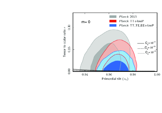
Figure 2: The upper and lower panels show the evolution of the tensor-to-scalar ratio $r$ versus the scalar spectral index $n_{s}$ in the weak dissipative regime for the special case $m=0$ ($\Gamma\propto\phi$), for different values of the parameter $C_{\phi}$. In both panels, the solid, dotted, and dashed lines correspond to the pairs ($A=0.47$, $f=0.29$), ($A=0.43$, $f=0.28$) and($A=0.39$, $f=0.29$), respectively. Also, in both panels we have used the values $C_{\gamma}=70$, $m_{p}=1$, $\tau=10^{-14}$, and the two-dimensional marginalized constraints from Ref.BICEP (upper panel) and the new data from Planck 2015 Planck2015 (lower panel).

In Fig.(1) we show the evolution of the ratio $\Gamma/3H$ versus the scalar spectral index (upper panel) and the evolution of the ratio $T/H$ versus the the scalar spectral index (lower panel), in the weak dissipative regime for the specific case in which the dissipative coefficient is given by $\Gamma(\phi,T)=C_{\phi}\,T$, i.e., $m=1$. In both panels, we have used three different values of the parameter $C_{\phi}$. The upper panel shows the condition for the weak dissipative regime in which $\Gamma<3H$. In the lower panel we show the necessary condition for warm inflation scenario, in which the temperature $T>H$. Combining Eqs.(1), (13) and (14), we numerically find the ratio $\Gamma/3H$ as a function of the scalar spectral index $n_{s}$. Analogously, from Eqs.(1) and (11), we numerically obtain the ratio between the temperature of the thermal bath $T$ and the Hubble parameter $H$, i.e., $T/H$ in terms of the spectral index $n_{s}$. In both plots, we consider the values $C_{\gamma}=70$, $m_{p}=1$ and $\tau=10^{-7}$. Also, numerically from Eqs.(21) and (23), we obtain the values $A=0.19$ and $f=0.31$ corresponding to the value of the parameter $C_{\phi}=10^{-2}$, for the values ${\mathcal{P}_{\mathcal{R}}}=2.43\times 10^{-9}$, $n_{s}=0.96$, and the number of $e$-folds $N=60$. Analogously, for the value $C_{\phi}=10^{-4}$, the values obtained for the parameters $A$ and $f$ are given by $A=0.28$ and $f=0.32$, respectively. Finally,for the value $C_{\phi}=10^{-6}$, we obtain the values $A=0.32$ and $f=0.30$. From the upper plot, we find an upper bound for the parameter $C_{\phi}$, from the condition of the weak dissipative regime, i.e., $\Gamma<3H$, for which $C_{\phi}\leq 10^{-2}$. From the lower panel we obtain a lower bound for $C_{\phi}$, considering the essential condition for warm inflation $T>H$, where $C_{\phi}\geq 10^{-6}$. In relation to the consistency relation $r=r(n_{s})$, we find that the ratio $r\sim 0$ for this range of $C_{\phi}$, then the case $m=1$ (or equivalently $\Gamma\propto T$) during the weak dissipative regime is disproved from BICEP2 experiment, because $r=0.2_{-0.05}^{+0.07}$ and further the ratio $r=0$ is discarded at 7.0$\sigma$. However, the Planck data analysis obtained only an upper limit for the tensor-to-scalar ratio $r$, given by $r<0.11$, and then the range of $C_{\phi}$ is well corroborated from Planck satellite. In this form, for the specific case of $m=1$, the range of the parameter $C_{\phi}$ is given by $10^{-6}\leq C_{\phi}\leq 10^{-2}$. Also, we note that when we decrease the value of the parameter $C_{\phi}<10^{-6}$, the value of the tensor to scalar ratio $r\simeq 0$. In particular, for the value $C_{\phi}=10^{-6}$, we get $r\mid_{n_{s}=0.96}\simeq 7\times 10^{-4}$. It is interesting to note that the range for the parameter $C_{\phi}$ for the case $\Gamma\propto T$ results from the conditions $\Gamma<3H$ and $T>H$.

In Fig.(2) we show the tensor-to-scalar ratio $r$ versus the scalar spectral index $n_{s}$, for the special case of $m=0$, i.e., $\Gamma\propto\phi$ in the weak dissipative regime ($\Gamma<3H$). In the upper panel we show the two-dimensional marginalized constraints for the tensor-to-scalar ratio $r=r(n_{s})$ (at 68$\%$ and 95$\%$ levels of confidence), from the BICEP2 experiment data in connection with Planck satellite+ WP+ highLBICEP . In the lower panel the new results from Planck 2015Planck2015 . Here, the marginalized joint 68$\%$ and 95$\%$ CL regions for the spectral index $n_{s}$ and $r_{0.002}$. From Eqs.(23) and (25), we numerically obtain the consistency relation $r=r(n_{s})$ and, as before, we consider three values of the parameter $C_{\phi}$. Again, we take the values $C_{\gamma}=70$, $m_{p}=1$ and $\tau=10^{-14}$. From these plots we observe that the tensor-to -scalar ratio $r\sim 0$ for the specific case of $m=0$, and then this case is disproved from BICEP2 experiment (upper panel), however is well corroborated from Planck data and in special with the new data (lower panel). We observe that the new results from Planck 2015 place more substantial limits on the consistency relation $r=r(n_{s})$ compared with the BICEP2 experiment.

In particular for the value of $C_{\phi}=10^{-21}$ (solid line in the figure), we get that $r\mid_{n_{s}=0.96}\simeq 2\times 10^{-3}$. From the essential condition for warm inflation $T>H$, we find a lower limit for the parameter $C_{\phi}$ given by $C_{\phi}\geq 10^{-21}$ and, considering the condition of weak dissipative regime, where $\Gamma<3H$, we obtain un upper bound for $C_{\phi}$, and it corresponds to $C_{\phi}\leq 10^{-15}$ (figure not shown). In this form, for the special case of $m=0$ (or equivalently $\Gamma\propto\phi$), the range for the parameter $C_{\phi}$ is given by $10^{-21}\leq C_{\phi}\leq 10^{-15}$.

For the cases $m=3$ and $m=-1$, we find that the tensor-to-scalar ratio $r\sim 0$, then these cases are disproved from BICEP2 data, nevertheless are well corroborated from Planck satellite and Planck 2015 data. Considering the essential condition for warm inflation $T>H$, we obtain a lower bound for the parameter $C_{\phi}$; for the case $m=3$ the bound is $10^{22}\leq C_{\phi}$ and for the case $m=-1$ it corresponds to $10^{-34}\leq C_{\phi}$. In particular, for the value $C_{\phi}=10^{22}$ corresponds to $\left(\frac{T}{H}\right)\mid_{n_{s}=0.96}\simeq 1.86$ when $m=3$, and for $C_{\phi}=10^{-34}$ corresponds to $\left(\frac{T}{H}\right)\mid_{n_{s}=0.96}\simeq 1.57$ for the case $m=-1$. From the condition of weak dissipative regime $\Gamma<3H$, we find an upper bound for $C_{\phi}$; for the case $m=3$ the upper bound is $C_{\phi}\leq 10^{23}$, and for the specific case $m=-1$, results $C_{\phi}\leq 10^{-28}$. In particular, for the value $C_{\phi}=10^{23}$ corresponds to $\left(\frac{\Gamma}{3H}\right)\mid_{n_{s}=0.96}\simeq 0.44$ when $m=3$, and for $C_{\phi}=10^{-28}$ corresponds to $\left(\frac{\Gamma}{3H}\right)\mid_{n_{s}=0.96}\simeq 0.18$ for the case $m=-1$. In this form, from the conditions $T>H$ and $\Gamma<3H$, the ranges for the parameter $C_{\phi}$, are given by: $10^{22}\leq C_{\phi}\leq 10^{23}$ for the case $m=3$, and $10^{-34}\leq C_{\phi}\leq 10^{-28}$ for the case $m=-1$.

II.2 The strong dissipative regime.

Now we consider the case of strong dissipative regime $R>1$ (or equivalently $\Gamma>3H$), together with the scalar factor $a(t)$ of intermediate inflation, see Eq.(1). Considering Eqs. (8) and (13), we find the solution for the scalar field $\phi(t)$. In particular, we must to analyze our solution for two separate cases, namely $m=3$ and $m\neq 3$. For the special case of $m=3$, the solution for the scalar field results

$$\phi(t)-\phi_{0}=\frac{\tilde{B}[t]}{\tilde{K}},$$ (26)

as before, the value of $\phi(t=0)=\phi_{0}$ is an integration constant and $\tilde{K}$ is a constant given by

$$\tilde{K}\equiv\left(\frac{4C_{\phi}}{\tau}\right)^{1/2}\left(\frac{1}{2\kappa C_{\gamma}}\right)^{3/8}\left[\left(\frac{\kappa\tau}{2}\right)^{\frac{4-3(f-2)}{2(1-f)}}\left(\frac{(1-f)^{1-f}}{Af}\right)^{7}\right]^{1/8(1-f)},$$

and $\tilde{B}[t]$ is a new function that is defined as

$$\tilde{B}[t]\equiv B\left[-\frac{\kappa\tau}{2(Af)^{2}}t^{2(1-f)};\,\frac{4f+3}{16(1-f)},\,\frac{15}{16}\right],$$ (27)

and corresponds to the incomplete beta functionLibro .

On the other hand, the solution of the scalar field for the special case $m\neq 3$ yields

$$\varphi(t)-\varphi_{0}=\frac{\tilde{B}_{m}[t]}{\tilde{K}_{m}},$$ (28)

here the scalar field $\phi(t)$ is redefined as $\varphi(t)=\frac{2}{3-m}\phi(t)^{\frac{2}{3-m}}$ and as before $\varphi_{0}$ is an integration constant, that can be assumed $\varphi_{0}=0$. The quantity $\tilde{K}_{m}$ is a new constant given by $\tilde{K}_{m}\equiv\left(\frac{4C_{\phi}}{\tau}\right)^{1/2}\left(\frac{1}{2\kappa C_{\gamma}}\right)^{m/8}\left[\left(\frac{\kappa\tau}{2}\right)^{\frac{4-m(f-2)}{2(1-f)}}\left(\frac{(1-f)^{1-f}}{Af}\right)^{4+m}\right]^{1/8(1-f)}$, and the new function $\tilde{B}_{m}[t]$ for the special case in which $m\neq 3$ is defined as

$$\tilde{B}_{m}[t]\equiv B\left[-\frac{\kappa\tau}{2(Af)^{2}}t^{2(1-f)};\,\frac{4f+m}{16(1-f)},\,\frac{12+m}{16}\right].$$ (29)

From Eqs.(1), (26) and (28), we find that the Hubble parameter $H=H(\phi)$ yields

$$H(\phi)=\frac{Af}{(\tilde{B}^{-1}[\tilde{K}\ln\phi])^{1-f}},\,\,\;\text{for}\,m=3,$$ (30)

and for the special case of $m\neq 3$ we have

$$H(\phi)=\frac{Af}{(\tilde{B}_{m}^{-1}[\tilde{K}_{m}\varphi])^{1-f}}.$$ (31)

By considering Eq.(12) , the scalar potential under the slow-roll approximation for both values of $m$ is given by

$$V(\phi)=\tau\left(-1+\left[1+\frac{2A^{2}f^{2}}{\kappa\tau(\tilde{B}^{-1}[\tilde{K}\ln\phi])^{2(1-f)}}\right]^{1/2}\right),$$ (32)

for the special case $m=3$, and

$$V(\phi)=\tau\left(-1+\left[1+\frac{2A^{2}f^{2}}{\kappa\tau(\tilde{B}_{m}^{-1}[\tilde{K}_{m}\varphi])^{2(1-f)}}\right]^{1/2}\right),$$ (33)

for the value of $m\neq 3$.

The dissipative coefficient $\Gamma$ in terms of the scalar field, can be obtained combining Eqs. (13), (26), and (28) to give

$$\Gamma(\phi)=\delta\phi^{-2}(\tilde{B}^{-1}[\tilde{K}\ln\phi])^{-\frac{3(2-f)}{4}}\left[1+\frac{2H^{2}}{\kappa\tau}\right]^{-3/8},$$ (34)

for the case $m=3$, in which the constant $\delta$ is defined as $\delta=C_{\phi}\left[\frac{Af(1-f)}{2\kappa C_{\gamma}}\right]^{3/4}$. For the value of $m\neq 3$ we find

$$\Gamma(\phi)=\delta_{m}\phi^{1-m}(\tilde{B}_{m}^{-1}[\tilde{K}_{m}\varphi])^{-\frac{m(2-f)}{4}}\left[1+\frac{2H^{2}}{\kappa\tau}\right]^{-m/8},$$ (35)

where $\delta_{m}$ is a constant and is given by $\delta_{m}=C_{\phi}\left[\frac{Af(1-f)}{2\kappa C_{\gamma}}\right]^{m/4}$.

Analogous to the case of the weak dissipative regime, the dimensionless slow-roll parameter $\varepsilon$ is given by $\varepsilon=-\frac{\dot{H}}{H^{2}}=\frac{1-f}{Af(\tilde{B}^{-1}[\tilde{K}\ln\phi])^{f}}$, for $m=3$ and for the value of $m\neq 3$ we find $\varepsilon=\frac{1-f}{Af(\tilde{B}_{m}^{-1}[\tilde{K}_{m}\varphi])^{f}}$. Again, if $\ddot{a}>0$, then the scalar field $\phi>\exp[\frac{1}{\tilde{K}}\tilde{B}[(\frac{1-f}{Af})^{1/f}]]$, for the special case $m=3$, and for the case $m\neq 3$ the new scalar field satisfied $\varphi>\frac{1}{\tilde{K}_{m}}\tilde{B}_{m}[(\frac{1-f}{Af})^{1/f}]$. Analogously as before, the inflationary scenario begins ($\varepsilon=1$) when the scalar field takes the value $\phi_{1}=\exp[\frac{1}{\tilde{K}}\tilde{B}[(\frac{1-f}{Af})^{1/f}]]$, for $m=3$, and $\varphi_{1}=\frac{1}{\tilde{K}_{m}}\tilde{B}_{m}[(\frac{1-f}{Af})^{1/f}]$ for the special case of $m\neq 3$.

The number of e-folds $N$ in this regime can be write using Eqs.(1), (26), and (28), to give

$$N=\int_{t_{1}}^{t_{2}}\,H\,dt=A[(\tilde{B}^{-1}[\tilde{K}\ln\phi_{2}])^{f}-(\tilde{B}^{-1}[\tilde{K}\ln\phi_{1}])^{f}],$$ (36)

for the case of $m=3$, and for the special case of $m\neq 3$ we have

$$N=A[(\tilde{B}_{m}^{-1}[\tilde{K}_{m}\varphi_{2}])^{f}-(\tilde{B}_{m}^{-1}[\tilde{K}_{m}\varphi_{1}])^{f}].$$ (37)

Analogous to the case of the weak dissipative regime, now we will analyze the cosmological perturbations in which $R=\Gamma/3H>1$ (strong dissipative regime). For the strong dissipative regime, the fluctuations $\delta\phi^{2}$ is given by $\delta\phi^{2}\simeq\frac{k_{F}T}{2\pi^{2}}$, see Ref.warm , where $k_{F}$ corresponds to the wave-number and it is determined as $k_{F}=\sqrt{\Gamma H}=H\sqrt{3R}>H$. In this way, the power spectrum of the scalar perturbation in this regime from Eqs.(1), (11) and (13), can be written as

$$P_{\mathcal{R}}\simeq\frac{H^{\frac{5}{2}}\Gamma^{\frac{1}{2}}T}{2\pi^{2}\dot{\phi}^{2}}=\frac{\kappa}{4\pi^{2}}C_{\phi}^{3/2}\phi^{\frac{3(1-m)}{2})}H^{3/2}(-\dot{H})^{\frac{3m-6}{8}}\left[1+\frac{2H^{2}}{\kappa\tau}\right]^{-\frac{(3m-6)}{16}}.$$ (38)

Analogously as before, we can find the power spectrum $\mathcal{P}_{\mathcal{R}}$ in terms of the scalar field $\phi$ for both values of the parameter $m$. In this form, considering Eqs. (1), (26), (28) and Eq. (38) yields

$$\mathcal{P}_{\mathcal{R}}=k(\tilde{B}^{-1}[\tilde{K}\ln\phi])^{\frac{3(5f-6)}{8}}\phi^{-3}\left[1+\frac{2(Af)^{2}(\tilde{B}^{-1}[\tilde{K}\ln\phi])^{-2(1-f)}}{\kappa\tau}\right]^{-3/16},$$ (39)

for the case of $m=3$. Here the constant $k$ is given by $k=\frac{k}{4\pi^{2}}C_{\phi}^{3/2}\left(\frac{1}{2\kappa C_{\gamma}}\right)^{11/8}(Af)^{15/8}(1-f)^{3/8}$.

Now, the spectrum of the scalar perturbation for the special case of $m\neq 3$, results

$$\mathcal{P}_{\mathcal{R}}=k_{m}(\tilde{B}_{m}^{-1}[\tilde{K}_{\varphi}])^{\frac{3[f(2+m)-2m]}{8}}\phi^{\frac{3(1-m)}{2}}\left[1+\frac{2(Af)^{2}(\tilde{B}_{m}^{-1}[\tilde{K}_{m}\varphi])^{-2(1-f)}}{\kappa\tau}\right]^{-\frac{(3m-6)}{16}},$$ (40)

where $k_{m}$ is a constant given by $k_{m}=\frac{k}{4\pi^{2}}C_{\phi}^{3/2}\left(\frac{1}{2\kappa C_{\gamma}}\right)^{\frac{3m+2}{8}}(Af)^{\frac{3m+6}{8}}(1-f)^{\frac{3m-6}{8}}$.

Also, the scalar power spectrum can be rewritten in terms of the number of $e$-folds $N$. From Eqs.(36) and (37), the power spectrum $\mathcal{P}_{\mathcal{R}}$ becomes

$$\mathcal{P}_{\mathcal{R}}=k(J[N])^{\frac{3(5f-6)}{8}}\exp\left(-\frac{\tilde{B}[J[N]]}{\tilde{K}}\right)\left[1+\frac{2(Af)^{2}(J[N])^{-2(1-f)}}{\kappa\tau}\right]^{-3/16},$$ (41)

for the specific case of $m=3$, and for the case $m\neq 3$ we have

$$\mathcal{P}_{\mathcal{R}}=\tilde{\gamma}_{m}(J[N])^{\frac{3[f(2+m)-2m]}{8}}(\tilde{B}_{m}[J[N]])^{\frac{3(1-m)}{3-m}}\left[1+\frac{2(Af)^{2}(J[N)^{-2(1-f)}}{\kappa\tau}\right]^{-\frac{(3m-6)}{16}},$$ (42)

where the constant $\tilde{\gamma}_{m}$ in the above equation is given by $\tilde{\gamma}_{m}=k_{m}\left(\frac{2\tilde{K}_{m}}{3-m}\right)^{-\frac{3(1-m)}{3-m}}$.

For this regime the scalar spectral index $n_{s}$ for the specific case of $m=3$ from Eqs. (39) and (40) results

$$n_{s}=1+\frac{3(5f-6)}{8Af}(\tilde{B}^{-1}[\tilde{K}\ln\phi])^{-f}+n_{1}+n_{2}.$$ (43)

Here the new functions $n_{1}$ and $n_{2}$ are given by $n_{1}=-3\left(\frac{2}{\kappa}\right)^{1/2}\frac{1}{C_{\phi}^{1/2}}\left(\frac{1}{2\kappa C_{\gamma}}\right)^{-3/8}(Af)^{-3/8}\\ \times(1-f)^{1/8}\left[1+\frac{2(Af)^{2}(\tilde{B}^{-1}[\tilde{K}\ln\phi])^{-2(1-f)}}{\kappa\tau}\right]^{-1/16}$ and $n_{2}=\frac{3Af(1-f)}{4\kappa\tau}(\tilde{B}^{-1}[\tilde{K}\ln\phi])^{f-2}\\ \times\left[1+\frac{2(Af)^{2}(\tilde{B}^{-1}[\tilde{K}\ln\phi])^{-2(1-f)}}{\kappa\tau}\right]^{-1}$, respectively. By other hand, the scalar spectral index for the case $m\neq 3$ becomes

$$n_{s}=1+\frac{3[f(m+2)-2m]}{8Af}(\tilde{B}_{m}^{-1}[\tilde{K}_{m}\varphi])^{-f}+n_{1_{m}}+n_{2_{m}},$$ (44)

where now the new functions $n_{1_{m}}$ and $n_{2_{m}}$ are defined by $n_{1_{m}}=\frac{3(1-m)}{2Af}\left(\frac{2}{\kappa}\right)^{1/2}\left(\frac{1}{2\kappa C_{\gamma}}\right)^{-m/8}\\ \times\frac{1}{C_{\phi}^{1/2}}(Af)^{\frac{8-m}{8}}(1-f)^{\frac{4-m}{8}}(\tilde{B}_{m}^{-1}[\tilde{K}_{m}\varphi])^{-\frac{[4+m(f-2)]}{8}}\phi^{\frac{m-3}{2}}\left[1+\frac{2(Af)^{2}(\tilde{B}_{m}^{-1}[\tilde{K}_{m}\varphi])^{-2(1-f)}}{\kappa\tau}\right]^{\frac{m-4}{16}}$ and $n_{2_{m}}=\frac{(3m-6)}{4\kappa\tau}(Af)(1-f)(\tilde{B}_{m}^{-1}[\tilde{K}_{m}\varphi])^{f-2}\left[1+\frac{2(Af)^{2}(\tilde{B}_{m}^{-1}[\tilde{K}_{m}\varphi])^{-2(1-f)}}{\kappa\tau}\right]^{-1}$.

Analogously as before, from Eqs.(36) and (37), the scalar spectral index $n_{s}$ can be rewritten in terms of the number of $e$-folds as

$$n_{s}=1+\frac{3(5f-6)}{8Af}(J[N])^{-f}+n_{1}+n_{2},$$ (45)

for the specific case of $m=3$. Here the quantities $n_{1}(J[N])$ and $n_{2}(J[N])$ are defined as $n_{1}(J[N])=-3\left(\frac{2}{\kappa}\right)^{1/2}\frac{1}{C_{\phi}^{1/2}}\left(\frac{1}{2\kappa C_{\gamma}}\right)^{-3/8}(Af)^{-3/8}(1-f)^{1/8}\left[1+\frac{2(Af)^{2}(J[N])^{-2(1-f)}}{\kappa\tau}\right]^{-1/16}$ and $n_{2}(J[N])=\frac{3Af(1-f)}{4\kappa\tau}(J[N])^{f-2}\left[1+\frac{2(Af)^{2}(J[N])^{-2(1-f)}}{\kappa\tau}\right]^{-1}$, respectively. Analogously, the scalar spectral index for the value of $m\neq 3$ yields

$$n_{s}=1+\frac{3[f(m+2)-2m]}{8Af}(J[N])^{-f}+n_{1_{m}}+n_{2_{m}},$$ (46)

where $n_{1_{m}}(J[N])=\frac{6(1-m)}{3-m}\left(\frac{\kappa}{2}\right)^{\frac{[f(16-m)+2(m-6)]}{16(1-f)}}(Af)^{-\frac{[4+m(2-f)]}{8(1-f)}}\left[1+\frac{2(Af)^{2}(J[N])^{-2(1-f)}}{\kappa\tau}\right]^{\frac{m-4}{16}}\\ \times(J[N])^{-\frac{[4+m(f-2)]}{8(1-f)}}(\tilde{B}_{m}[J[N]])^{-1}$ and $n_{2_{m}}(J[N])=\frac{(3m-6)}{4\kappa\tau}(Af)(1-f)(J[N])^{f-2}\\ \times\left[1+\frac{2(Af)^{2}(J[N])^{-2(1-f)}}{\kappa\tau}\right]^{-1}$.

Analogous to the case of the weak dissipative regime, the tensor-to-scalar-ratio $r$ for the specific case $m=3$ can be expressed in terms of the scalar field to give

$$r=\frac{6\kappa}{\pi^{2}k}(Af)^{2}(\tilde{B}^{-1}[\tilde{K}\ln\phi])^{\frac{(f+2)}{8}}\phi^{3}\left[1+\frac{2(Af)^{2}(\tilde{B}^{-1}[\tilde{K}\ln\phi])^{-2(1-f)}}{\kappa\tau}\right]^{\frac{3}{16}}F^{2}(\phi),$$ (47)

and the tensor-to-scalar-ratio for the case $m\neq 3$ yields

$$r=\frac{6\kappa}{\pi^{2}k_{m}}(Af)^{2}(\tilde{B}_{m}^{-1}[\tilde{K}_{m}\varphi])^{\frac{1}{8}[6m+f(10-3m)-16]}\phi^{\frac{3}{2}(m-1)}\,\,\;\times$$

$$\left[1+\frac{2(Af)^{2}(\tilde{B}_{m}^{-1}[\tilde{K}_{m}\varphi])^{-2(1-f)}}{\kappa\tau}\right]^{\frac{(3m-6)}{16}}F^{2}(\phi).$$ (48)

Also, we obtain the tensor-to-scalar ratio in terms of the number of $e$-folds. In this form, combining Eqs.(36) and (47) we get

$$r=\frac{6\kappa}{\pi^{2}k}(Af)^{2}(J[N])^{\frac{(f+2)}{8}}\exp\left[3\frac{\tilde{B}[J[N]]}{\tilde{K}}\right]\left[1+\frac{2(Af)^{2}(J[N])^{-2(1-f)}}{\kappa\tau}\right]^{\frac{3}{16}}F^{2}(N),$$ (49)

for the specific case of $m=3$. From Eqs.(37) and (48), the tensor to scalar ratio becomes

$$r=\frac{6\kappa}{\pi^{2}k_{m}}(Af)^{2}(J[N])^{\frac{1}{8}[6m+f(10-3m)-16]}\left(\frac{3-m}{2}\frac{\tilde{B}_{m}[J[N]]}{\tilde{K}_{m}}\right)^{\frac{3(m-1)}{3-m}}\,\,\times$$

$$\left[1+\frac{2(Af)^{2}(J[N])^{-2(1-f)}}{\kappa\tau}\right]^{\frac{(3m-6)}{16}}F^{2}(N),$$ (50)

for the case of $m\neq 3$.

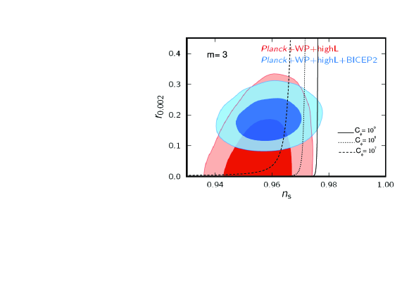
Figure 3: The evolution of the tensor-to-scalar ratio $r$ (upper panel) and the evolution of the ratio $\Gamma/3H$ versus the scalar spectral index $n_{s}$ (lower panel) in the strong dissipative regime, for the special case $m=3$ ($\Gamma\propto T^{3}/\phi^{2}$) for three different values of the parameter $C_{\phi}$. In both panels, the solid, dotted, and dashed lines correspond to the pairs ($A=1.32\times 10^{-5}$, $f=0.75$), ($A=7.68\times 10^{-6}$, $f=0.87$) and ($A=5.40\times 10^{-6}$, $f=0.97$). In both panels we have used the values $C_{\gamma}=70$, $m_{p}=1$, $\tau=10^{-14}$, and the two-dimensional marginalized constraints from Ref.BICEP .

In Fig.(3) we show the evolution of the tensor-to-scalar ratio $r$ and the ratio $\Gamma/3H$ on the spectral index $n_{s}$ in the strong dissipative regime, for the special case in which $\Gamma=C_{\phi}\,T^{3}/\phi^{2}$, i.e., $m=3$. In both panels we have used three different values of the parameter $C_{\phi}$. In the upper panel, as before, we show the two-dimensional constraints in the $n_{s}$-$r$ plane from BICEP2 and Planck data ($68\%$ and $95\%$ levels of confidence)BICEP . In the lower panel we show the evolution of the ratio $\Gamma/3H$ during the warm inflation scenario, and we corroborate that our model satisfies the strong dissipative regime, i.e., $\Gamma>3H$. In order to write down the consistency relation $r=r(n_{s})$, we numerically find from Eqs.(45) and (49), the relation $r=r(n_{s})$ (upper panel). Similarly, from Eqs.(34), (37) and (45) we obtain the ratio $\Gamma/3H$ as a function of the spectral index $n_{s}$ (lower panel). In these plots we consider the values of $C_{\gamma}=70$, $m_{p}=1$ and $\tau=10^{-14}$. Also, numerically from Eqs.(41) and (45) for the special case of $m=3$, we obtain the values $A=1.32\times 10^{-5}$ and $f=0.75$ corresponding to the value $C_{\phi}=10^{9}$, for $P_{\mathcal{R}}=2.43\times 10^{-9}$, $n_{s}=0.96$ and $N=60$. Analogously, for the parameter $C_{\phi}=10^{8}$, we numerically find the the values $A=7.68\times 10^{-6}$ and $f=0.87$. Finally, for the value $C_{\phi}=10^{7}$ we obtain $A=5.40\times 10^{-6}$ and $f=0.97$. From the upper panel we obtain that the range for the parameter $C_{\phi}$ is $10^{7}\leq C_{\phi}\leq 10^{9}$, which is well supported from observational data. However, from the lower panel we observe that for values of $C_{\phi}\leq 10^{8}$ the model is disapproved from the condition the strong dissipative regime, since the ratio $\Gamma/3H<1$. Here, we note that from the condition of the strong dissipative regime, i.e., $\Gamma>3H$, we have obtained a lower bound for the parameter $C_{\phi}$. In this form, for the value $m=3$ ( in which $\Gamma\propto T^{3}/\phi^{2}$) the range for the parameter $C_{\phi}$ is given by $10^{8}\leq C_{\phi}\leq 10^{9}$, which is well supported from observational data together with the conditions of the strong dissipative regime $\Gamma>3H$ and $T>H$.

During the strong dissipative regime for the specific case of $m=1$ ($\Gamma\propto T$) , we obtain that for the value of the parameter $C_{\phi}\geq 10^{-1}$ the model is well corroborated from the condition $\Gamma>3H$ and the necessary condition for warm inflation $T>H$ (figure not shown). For the tensor-to-scalar ratio, we find that the ratio $r\sim 0$ for this lower bound, then the case $m=1$ is disproved from BICEP2 experiment, since the ratio $r=0$ is discarded at 7.0$\sigma$. However, from the Planck data, the value $C_{\phi}\geq 10^{-1}$ is well supported. Also, we note that when we increase the value of the parameter $C_{\phi}>10^{-1}$, the value of the tenso-to-scalar ratio $r\simeq 0$.

For the cases $m=0$ ($\Gamma\propto\phi$) and $m=-1$ ($\Gamma\propto\phi^{2}/T$), we find that these models in the strong dissipative models are disproved from BICEP2 and Planck data, because the scalar spectral index $n_{s}>1$, and then these models do not work.

III Conclusions

In this paper we have studied warm-intermediate inflation in the context of Randall-Sundrum II brane-world cosmological model. Considering the slow-roll approximation during the weak and strong regime, we have obtained analytical solutions of the full effective Friedmann equation for a flat Universe in this brane-world model. Here we have considered a standard scalar field $\phi$ together with a general form of the dissipative coefficient $\Gamma\propto\,T^{m}/\phi^{m-1}$. In special, we analyzed the values $m=3$, $m=1$, $m=0$ and $m=-1$, that can be have found in the literature for this dissipation coefficient. Studying the weak and strong dissipative regimes, we have obtained analytical expressions for the appropriate Hubble parameter, effective potential, scalar power spectrum, scalar spectral index and the tensor-to-scalar ratio. During both regimes we have studied the slow roll analysis and we compared with the two-dimensional marginalized constraints (68$\%$ and 95$\%$ C.L.) $r=r(n_{s})$ plane from observational data. Also, we have obtained a constraint for the parameter $C_{\phi}$ (see Eq.6) from BICEP2 and Planck 2015 data together with the essential condition for warm inflation $T>H$ and the condition from the weak $\Gamma<3H$ (or strong $\Gamma>3H$) regime.

For all the models (different values of the parameter $m$) in the weak dissipative regime, we have found a lower bound for the parameter $C_{\phi}$, from the essential condition for warm inflation, in which the temperature of the thermal bath $T>H$. Also, we have obtained an upper bound for $C_{\phi}$, from the condition $\Gamma<3H$, i.e., the weak dissipative regime. Additionally, we have observed that the consistency relation $r=r(n_{s})\sim 0$, in the weak dissipative scenario, and the models are disproved from BICEP2, but are well corroborated from Planck satellite, since $r<0.11$.

For the strong dissipative scenario, we have found that the range for the parameter $C_{\phi}$ is given by $10^{8}\leq C_{\phi}\leq 10^{9}$ in the specific case of $m=3$ i.e., $\Gamma\propto T^{3}/\phi^{2}$. Here, we have found an upper bound from BICEP2-Planck $r-n_{s}$ plane and a lower bound from the condition of the dissipative regime in which $\Gamma>3H$, also in this range of $C_{\phi}$ the necessary condition for warm inflation $T>H$ is satisfied. For the case $m=1$ ($\Gamma\propto T$), we have obtained that the tensor-to-scalar ratio $r\sim 0$, and also we have found a lower limit for the parameter $C_{\phi}$ from the condition $\Gamma>3H$. Finally, we have found that for the cases $m=0$ and $m=-1$, these warm-intermediate inflationary models are disproved from observational data, since the scalar spectral index $n_{s}>1$, then the models $\Gamma\propto\phi$ and $\Gamma\propto\phi^{2}/T$ do not work.

- (1) A. Guth , Phys. Rev. D 23, 347 (1981)
- (2) A.A. Starobinsky, Phys. Lett. B 91, 99 (1980)
- (3) A.D. Linde, Phys. Lett. B 108, 389 (1982)
- (4) A.D. Linde, Phys. Lett. B 129, 177 (1983)
- (5) A. Albrecht and P. J. Steinhardt, Phys. Rev. Lett. 48,1220 (1982)
- (6) K. Sato, Mon. Not. Roy. Astron. Soc. 195, 467 (1981).
- (7) V.F. Mukhanov and G.V. Chibisov , JETP Letters 33, 532(1981)
- (8) S. W. Hawking,Phys. Lett. B 115, 295 (1982)
- (9) A. Guth and S.-Y. Pi, Phys. Rev. Lett. 49, 1110 (1982)
- (10) A. A. Starobinsky, Phys. Lett. B 117, 175 (1982)
- (11) J.M. Bardeen, P.J. Steinhardt and M.S. Turner, Phys. Rev.D 28, 679 (1983).
- (12) D. Larson et al., Astrophys. J. Suppl. 192, 16 (2011).
- (13) C. L. Bennett et al., Astrophys. J. Suppl. 192, 17 (2011)
- (14) N. Jarosik et al., Astrophys. J. Suppl. 192, 14 (2011)
- (15) G. Hinshaw et al. [WMAP Collaboration], Astrophys. J. Suppl. 208, 19 (2013)
- (16) P. A. R. Ade et al. [Planck Collaboration], Astron. Astrophys. 571, A16 (2014)
- (17) P. A. R. Ade et al. [Planck Collaboration], Astron. Astrophys. 571, A22 (2014)
- (18) P. A. R. Ade et al. [Planck Collaboration], arXiv:1502.02114 [astro-ph.CO].
- (19) A. Berera, Phys. Rev. Lett. 75, 3218 (1995); A. Berera, Phys. Rev. D 55, 3346 (1997).
- (20) L.M.H. Hall, I.G. Moss and A. Berera, Phys.Rev.D 69, 083525 (2004).
- (21) A. Berera, Phys. Rev.D 54, 2519 (1996).
- (22) A. Berera, I. G. Moss and R. O. Ramos, Rept. Prog. Phys. 72, 026901 (2009); M. Bastero-Gil and A. Berera, Int. J. Mod. Phys. A 24, 2207 (2009).
- (23) A. Sen, JHEP 0204, 048 (2002).
- (24) K. Akama, Lect. Notes Phys. 176, 267 (1982); V. A. Rubakov and M. E. Shaposhnikov, Phys. Lett. B 159, 22 (1985); N. Arkani Hamed, S. Dimopoulos, and G. Dvali, Phys. Lett. B 429, 263 (1998); M. Gogberashvili, Europhys. Lett. 49, 396 (2000); L. Randall and R. Sundrum, Phys. Rev. Lett. 83, 3370 (1999); 83, 4690 (1999).
- (25) T. Shiromizu, K. Maeda, and M. Sasaki, Phys. Rev. D 62, 024012 (2000).
- (26) P. Binetruy, C. Deffayet, and D. Langlois, Nucl. Phys. B565, 269 (2000); P. Binetruy, C. Deffayet, U. Ellwanger, and D. Langlois, Phys. Lett. B 477, 285 (2000).
- (27) L. Randall and R. Sundrum, Phys.Rev.Lett.83, 4690 (1999).
- (28) L. Randall and R. Sundrum. Phys. Rev. Lett., 83, 3370, (1999).
- (29) W. D. Goldberger and M. B. Wise, Phys. Rev. Lett. 83, 4922 (1999); W. D. Goldberger and M. B. Wise, Phys. Lett. B 475, 275 (2000.
- (30) O. DeWolfe, D. Z. Freedman, S. S. Gubser and A. Karch, Phys. Rev. D 62, 046008 (2000); W. D. Goldberger and I. Z. Rothstein, Phys. Lett. B 491, 339 (2000); N. Arkani-Hamed, S. Dimopoulos and J. March-Russell, Phys. Rev. D 63, 064020 (2001). M. A. Luty and R. Sundrum, Phys. Rev. D 64, 065012 (2001); R. Hofmann, P. Kanti and M. Pospelov, Phys. Rev. D 63, 124020 (2001); J. Garriga, O. Pujolas and T. Tanaka, Nucl. Phys. B 605, 192 (2001); A. Flachi, I. G. Moss and D. J. Toms, Phys. Rev. D 64, 105029 (2001); S. Nojiri, S. D. Odintsov and S. Zerbini, Class. Quant. Grav. 17, 4855 (2000); I. Brevik, K. A. Milton, S. Nojiri and S. D. Odintsov, Nucl. Phys. B 599, 305 (2001).
- (31) T. Tanaka and X. Montes, Nucl. Phys. B 582, 259 (2000); S. Mukohyama and L. Kofman, Phys. Rev. D 65, 124025 (2002).
- (32) R. Maartens, D. Wands, B. A. Bassett, and I. P. C. Heard, Phys. Rev. D 62, 041301 (2000).
- (33) J. M. Cline, C. Grojean, and G. Servant, Phys. Rev. Lett.83, 4245 (1999).
- (34) P. Brax and C. van de Bruck, Class. Quant. Grav. 20, R201 (2003); ⁃ T. Clifton, P. G. Ferreira, A. Padilla and C. Skordis, Phys. Rept. 513, 1 (2012).
- (35) C. Csaki, M. Graesser, C. F. Kolda and J. Terning, Phys. Lett. B 462 34 (1999); D. Ida, JHEP 0009, 014 (2000); R. N. Mohapatra, A. Perez-Lorenzana, and C. A. de S. Pires, Phys. Rev. D 62, 105030 (2000); R. N. Mohapatra, A. Perez-Lorenzana, and C. A. de S. Pires, Int. J. Mod. Phys. A 16, 1431 (2001); Y. Gong, arXiv:gr-qc/0005075; R. Herrera, Phys. Lett. B 664, 149 (2008); Y. Ling and J. P. Wu, JCAP 1008, 017 (2010).
- (36) R. Maartens, arXiv:gr-qc/0101059.
- (37) F. Lucchin and S. Matarrese, Phys. Rev. D32, 1316 (1985).
- (38) J. D Barrow, Phys. Lett. B 235, 40 (1990); J. D Barrow and P. Saich, Phys. Lett. B 249, 406 (1990);A. Muslimov, Class. Quantum Grav. 7, 231 (1990); A. D. Rendall, Class. Quantum Grav. 22, 1655 (2005).
- (39) J. D Barrow and A. R. Liddle, Phys. Rev. D 47, R5219 (1993); A. A. Starobinsky JETP Lett. 82, 169 (2005); S. del Campo, R. Herrera, J. Saavedra, C. Campuzano and E. Rojas, Phys. Rev. D 80, 123531 (2009); R. Herrera and E. San Martin, Eur. Phys. J. C 71, 1701 (2011); R. Herrera and M. Olivares, Mod. Phys. Lett. A 27, 1250101 (2012); R. Herrera and M. Olivares, Int. J. Mod. Phys. D 21, 1250047 (2012).
- (40) W. H. Kinney, E. W. Kolb, A. Melchiorri and A. Riotto, Phys. Rev. D 74, 023502 (2006); R. Herrera and E. San Martin, Int. J. Mod. Phys. D 22, 1350008 (2013).
- (41) J. D. Barrow, A. R. Liddle and C. Pahud, Phys. Rev. D, 74, 127305 (2006); R. Herrera, M. Olivares and N. Videla, Eur. Phys. J. C 73, 2295 (2013).
- (42) T. Kolvisto and D. Mota, Phys. Lett. B 644, 104 (2007); Phys. Rev. D. 75, 023518 (2007).
- (43) I. Antoniadis, J. Rizos and K. Tamvakis, Nucl.Phys. B 415, 497 (1994).
- (44) D. G. Boulware and S. Deser, Phys.Rev. Lett. 55, 2656 (1985); Phys. Lett. B 175, 409 (1986).
- (45) S. Mignemi and N. R. Steward, Phys. Rev. D 47, 5259 (1993); P. Kanti, N. E. Mavromatos, J. Rizos, K. Tamvakis and E. Winstanley, Phys. Rev. D 54, 5049 (1996); Ch.M Chen, D. V. Gal’tsov and D. G. Orlov, Phys. Rev. D 75, 084030 (2007).
- (46) S. Nojiri, S. D. Odintsov and M. Sasaki, Phys. Rev. D 71, 123509 (2004); G. Gognola, E. Eizalde, S. Nojiri, S. D. Odintsov and E. Winstanley, Phys. Rev. D 73, 084007 (2006).
- (47) A. K. Sanyal, Phys. Lett. B, 645,1 (2007).
- (48) I. Antoniadis, J. Rizos and K. Tamvakis, Nucl. Phys. B. 415, 497 (1994); S. Nojiri, S. D. Odintsov and M. Sasaki, Phys. Rev. D. 71, 123509 (2004); G. Gognola, E. Eizalde, S. Nojiri, S. D. Odintsov and E. Winstanley, Phys. Rev. D. 73, 084007 (2006).
- (49) R. Herrera, N. Videla and M. Olivares, Phys. Rev. D 90, no. 10, 103502 (2014); R. Herrera, M. Olivares and N. Videla, Int. J. Mod. Phys. D 23, no. 10, 1450080 (2014); R. Herrera, M. Olivares and N. Videla, Phys. Rev. D 88, 063535 (2013); R. Herrera and E. San Martin, Int. J. Mod. Phys. D 22, 1350008 (2013). R. Herrera and E. San Martin, Eur. Phys. J. C 71, 1701 (2011).
- (50) P. A. R. Ade et al. (BICEP2 Collaboration), Phys. Rev. Lett. 112, 241101 (2014); Astrophys. J. 792, 62 (2014).
- (51) R. Adam et al. [Planck Collaboration], arXiv:1409.5738 [astro-ph.CO].
- (52) M. A. Cid, S. del Campo and R. Herrera, JCAP 0710, 005 (2007).
- (53) I. G. Moss and C. Xiong, arXiv:hep-ph/0603266.
- (54) A. Berera, M. Gleiser and R. O. Ramos, Phys. Rev. D 58 123508 (1998).
- (55) A. Berera and R. O. Ramos, Phys. Rev. D 63, 103509 (2001).
- (56) Y. Zhang, JCAP 0903, 023 (2009).
- (57) M. Bastero-Gil, A. Berera and R. O. Ramos, JCAP 1107, 030 (2011).
- (58) M. Bastero-Gil, A. Berera, R. O. Ramos and J. G. Rosa, JCAP 1301, 016 (2013); M. Bastero-Gil, A. Berera, R. O. Ramos and J. G. Rosa, arXiv:1404.4976 [astro-ph.CO].
- (59) S. Bartrum, M. Bastero-Gil, A. Berera, R. Cerezo, R. O. Ramos and J. G. Rosa, Phys. Lett. B 732, 116 (2014).
- (60) J. Yokoyama and A. Linde, Phys. Rev D 60, 083509, (1999); R. Herrera, M. Olivares and N. Videla, Phys. Rev. D 88, 063535 (2013).
- (61) M. Abramowitz and I. A. Stegun, Handbook of Mathemati- 733 cal Functions with Formulas, Graphs, and Mathematical 734 Tables, 9th ed. (Dover, New York, 1972); P. Appell and 735 J. Kampe de Feriet, Fonctions Hypergeeomeetriques et 736 Hyperspheeriques: Polynomes DHermite (Gauthier-Villars, 737 Paris, 1926); A. Erdelyi, Acta Math. 83, 131 (1964); H. 738 Exton, in Multiple Hypergeometric Functions and Appli- 739 cations (Wiley, New York, 1976).
- (62) D. Langlois, R. Maartens and D. Wands, Phys. Lett. B 489, 259 (2000).