Roton minimum as fingerprint of magnon-Higgs scattering in ordered quantum antiferromagnets

Abstract

A quantitative description of magnons in long-range ordered quantum antiferromagnets is presented which is consistent from low to high energies. It is illustrated for the generic $S=1/2$ Heisenberg model on the square lattice. The approach is based on a continuous similarity transformation in momentum space using the scaling dimension as truncation criterion. Evidence is found for significant magnon-magnon attraction inducing a Higgs resonance. The high-energy roton minimum in the magnon dispersion appears to be induced by strong magnon-Higgs scattering.

Introduction — The characterization of elementary excitations is of fundamental importance in condensed matter physics. Especially strongly correlated systems are known to host a large range of fascinating collective behavior leading to a zoo of exotic elementary quasi-particles with integer or non-integer, i.e, fractional, quantum numbers. The decay of integer excitations into fractional ones is called fractionalization. Prominent examples are the fractional quantum Hall effect with fractional charge excitations Laughlin (1983) or the physics of magnetic monopoles in spin ice where spin north and south poles move independently Castelnovo et al. (2008). Another arena of major importance is high-temperature superconductivity, where the nature of magnetic excitations has been intensively debated. The key point is whether fractional spin excitations, spinons with $S=1/2$, are present and essential Anderson (1987), or whether a description in terms of magnons or triplons with integer spin $S=1$ is appropriate Knetter et al. (2001).

Theoretically, the physics of undoped cuprates is closely related to the antiferromagnetic $S=1/2$ Heisenberg model on the two-dimensional (2D) square lattice Manousakis (1991). This paradigmatic unfrustrated model is known to display long-range Néel order with finite sublattice magnetization at zero temperature Reger and Young (1988); Chakravarty et al. (1989). The well-understood low-energy excitations are gapless magnons as enforced by Goldstone’s theorem Auerbach (1994).

Remarkably, the magnetic excitations at high energies are understood less well. But they have come into focus recently due to remarkable experimental progress in resolution Christensen et al. (2007); Dalla Piazza et al. (2015) and in the direct excitation at high energies Le Tacon et al. (2011). Conventional spin-wave (magnon) theory in powers of $1/S$ Hamer et al. (1992); Weihong and Hamer (1993); Igarashi and Nagao (2005); Syromyatnikov (2010); Uhrig and Majumdar (2013) fails to agree quantitatively with unbiased quantum Monte Carlo (QMC) simulations Sandvik and Singh (2001) and high-order series expansions about the Ising limit Sandvik and Singh (2001); Zheng et al. (2005). Even in third order in $1/S$, the approach based on magnons yields only a weak dip of the dispersion of about $3\%$ at $(\pi,0)$ compared to its value $(\pi/2,\pi/2)$ while series expansion and QMC yield about $10\%$. Inelastic neutron scattering (INS) finds $7(1)\%$ in deuterated copper formate Christensen et al. (2007); Dalla Piazza et al. (2015). In analogy to the similar feature in the dispersion of excitations in ⁴He Vollhardt and Wölfle (1990) we call this dip ‘roton minimum’.

The agreement of the INS data with the QMC and series results for the roton minimum on the one hand and the strong deviation of spin wave theory on the other hand have revived the idea, see, e.g., Ref. Ch.-M.Ho et al., 2001, that at high energies magnons are not the appropriate elementary excitations and that spinons provide a better description Dalla Piazza et al. (2015). The magnons at lower energies would result as confined states of spinon pairs Tang and Sandvik (2013) while the spinons are deconfined at least at certain points in the Brillouin zone (BZ) at higher energies.

The ambiguity between excitations having fractional or integer spin arises in gapless systems because without gap it is an ill-posed problem to determine the content of quasi-particles. This was for instance seen in one-dimensional (1D) spin chains Schmidt and Uhrig (2003). But in contrast to the 2D case, where magnons are the established Goldstone modes above the long-range ordered ground state, the 1D Heisenberg chain is known to display fractional massless spinons Faddeev and Takhtajan (1981). Consequently, a consistent determination of the full magnetic excitation spectrum for the 2D Heisenberg model from low to high energies is still missing, but highly desirable.

This is the central goal of the present Letter. We provide a quantitative description of the low- and the high-energy part of the dispersion in terms of magnons. Technically, this is achieved by extending continuous unitary transformations to continuous similarity transformations (CST) which are carried out in momentum space using the scaling dimensions of operators as appropriate truncation criterion.

Our results indicate a strong attractive magnon-magnon interaction. This interaction induces a Higgs resonance built from two-magnon states, also addressed as longitudinal magnon Lake et al. (2000); Rüegg et al. (2008); Pekker and Varma (2015). Thereby, significant weight in the three-magnon continuum is shifted towards lower energies and it can also be seen as magnon-Higgs continuum. These scattering states depress the single magnon states and reduce their energy yielding the roton minimum. In this way, this dip in the dispersion is a fingerprint of strong scattering between magnons and the damped Higgs mode.

2D Heisenberg model — We consider the Heisenberg quantum antiferromagnet on the square lattice

$$\mathcal{H}=J\sum_{\langle i,j\rangle}\vec{S}_{i}\cdot\vec{S}_{j}\quad,$$ (1)

where $\vec{S}_{i}$ denotes the vector operator of a spin $S=1/2$ at site $i$ and the sum runs over pairs of nearest neighbors. The ground state displays long-range Néel order. Consequently, the classical Néel state with spin up (spin down) on sublattice $A$ ($B$) serves as the appropriate reference state with respect to which bosonic operators create deviations. We use the non-hermitian Dyson-Maleev representation Dyson (1956); Maleev (1957) as is standard in analytic higher order calculations Hamer et al. (1992); Weihong and Hamer (1993); Igarashi and Nagao (2005); Syromyatnikov (2010); Uhrig and Majumdar (2013). Its asset is that the Hamiltonian only comprises terms that are at most quartic in the bosonic operators.

In this way, we obtain an initial Hamiltonian first in real space and by Fourier transformation in momentum space. A Bogoliubov transformation introducing $\alpha_{\bf k}^{(\dagger)}$ and $\beta_{\bf k}^{(\dagger)}$ as new bosonic operators yields Uhrig and Majumdar (2013); sup

$$\mathcal{H}=E_{0}+\sum_{{\bf k}}\omega_{{\bf k}}(\alpha^{\dagger}_{{\bf k}}\alpha^{\phantom{\dagger}}_{{\bf k}}+\beta^{\dagger}_{{\bf k}}\beta^{\phantom{\dagger}}_{{\bf k}})+\Gamma+\mathcal{V}.$$ (2)

The momenta ${\bf k}$ are taken from the magnetic BZ containing $N$ points given by the diamond with the four edges $(\pm\pi,0)$ and $(0,\pm\pi)$. The coefficients $E_{0}/N=-2J(S^{2}+AS+A^{2}/4)$ and $\omega_{{\bf k}}=2J(2S+A)\sqrt{1-\gamma_{{\bf k}}^{2}}$ with $\gamma_{{\bf k}}=(\cos k_{x}+\cos k_{y})/2$ and $A:=\frac{2}{N}\sum_{\bf k}(1-\sqrt{1-\gamma_{{\bf k}}^{2}})\approx 0.158$ correspond to the ground-state energy per site and the one-magnon dispersion in next-to-leading order spin-wave theory Hamer et al. (1992); Uhrig and Majumdar (2013). The Bogoliuov part $\Gamma:=\Gamma_{0}^{2}+\Gamma_{2}^{0}$ is bilinear; $\Gamma_{n}^{m}$ consists of $m$ creation and $n$ annihilation operators. The quartic terms are split according to $\mathcal{V}:=\mathcal{V}_{2}^{2}+\mathcal{V}_{1}^{3}+\mathcal{V}_{3}^{1}+\mathcal{V}_{0}^{4}+\mathcal{V}_{4}^{0}$ with the same pattern of bosonic operators. By construction, $\Gamma=0$ in (2) once the Bogoliubov transformation is carried out self-consistently. We define the part with more (less) creation than annihilation operators by $\mathcal{H}^{+}:=\Gamma_{0}^{2}+\mathcal{V}_{1}^{3}+\mathcal{V}_{0}^{4}$ ($\mathcal{H}^{-}:=\Gamma_{2}^{0}+\mathcal{V}_{3}^{1}+\mathcal{V}_{4}^{0}$).

Our goal is to derive an effective Hamiltonian $\mathcal{H}_{\rm eff}$ which conserves the number of magnons in order to simplify the subsequent analysis. We achieve this by extending the approach of CUTs Wegner (1994) to similarity transformations using the flow equation $\partial_{\ell}\mathcal{H}(\ell)=\left[\eta(\ell),\mathcal{H}(\ell)\right]$, where $\ell$ is a continuous auxiliary variable which labels the stage of the CUT: $\mathcal{H}(\ell)$ has the same structure as in (2), but all coefficients acquire a dependence on $\ell$. Initially, one has $\mathcal{H}(\ell=0)\ :=\mathcal{H}$ and finally $\mathcal{H}_{\rm eff}:=\mathcal{H}(\ell=\infty)$.

We use the generator $\eta(\ell):=\mathcal{H}^{+}(\ell)-\mathcal{H}^{-}(\ell)$ Knetter and Uhrig (2000); Fischer et al. (2010) leading to an effective Hamiltonian $\mathcal{H}_{\rm eff}$ that conserves the number of magnons. This is well-established for the converging flow of hermitian Hamiltonians and carries over to $\mathcal{H}$ in (2) because the Dyson-Maleev transformation does not mix states with different magnon number, but only attributes prefactors to them which spoil its unitarity. Summarizing, one maps the complicated many-body problem to an effective few-body Hamiltonian being block-diagonal in the number of magnons. The one-magnon block in particular is diagonal in momentum space after the CST so that the dispersion $\tilde{\omega}_{{\bf k}}$ can be read off.

Computing $\left[\eta(\ell),\mathcal{H}(\ell)\right]$ on the right hand side of the flow equation leads to a proliferating number of terms. One needs a systematically controlled truncation scheme to close the flow equation. So far, perturbative truncations have been used mostly Knetter and Uhrig (2000); Knetter et al. (2003); Kehrein (2006); Krull et al. (2012). In real space approaches the spatial range of processes is a related truncation criterion appropriate for gapped systems with finite correlation length Fischer et al. (2010); Yang and Schmidt (2011); Krull et al. (2012). In 1D, the scaling dimension was used in the operator product expansion of vertex operators Kehrein (1999, 2001). The criterion of the scaling dimension is particularly suitable for gapless systems with infinite correlation length. Hence, we apply this criterion for the 2D massless magnons.

We consider a generic term $\mathcal{T}$

$$\mathcal{T}\!\!=\!\!\int C_{{\bf k}_{1}\ldots{\bf k}_{n}}\mathcal{O}^{n}_{{\bf k}_{1}\ldots{\bf k}_{n}}\delta({\bf k}_{1}+\ldots+{\bf k}_{n})d^{2}{\bf k}_{1}\ldots d^{2}{\bf k}_{n},$$ (3)

where $\mathcal{O}^{n}_{{\bf k}_{1},\ldots{\bf k}_{n}}$ is a monomial of $n$ bosonic operators of creation or annihilation type . If we rescale all momenta ${\bf k}_{i}\rightarrow\lambda{\bf k}_{i}$ with $\lambda<1$ and assume that the coefficient is a homogeneous function $C_{\lambda{\bf k}_{1}\ldots\lambda{\bf k}_{n}}=\lambda^{c}C_{{\bf k}_{1}\ldots{\bf k}_{n}}$ the term $\mathcal{T}$ acquires a prefactor $\lambda^{n-2+c}$. The scaling dimension is the exponent $d:=n-2+c$. It quantifies the relevance of the term if we zoom to small energies in the sense of renormalization. Smaller scaling dimensions stand for more important terms. If the coefficient $C$ is not a homogeneous function we determine its dimensional contribution $c$ from the leading term in a series expansion in $\lambda$.

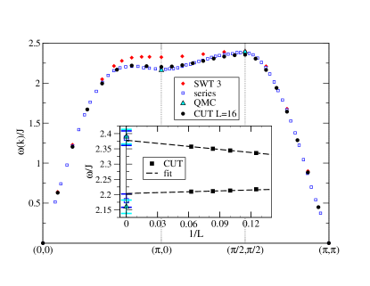
Figure 1: One-magnon dispersion $\omega({\bf k})$ in the magnetic BZ. Circles depict CST data for $L=16$; diamonds, squares, and triangles show data from spin-wave theory Syromyatnikov (2010), series expansion and QMC extrapolated to the thermodynamic limit Sandvik and Singh (2001). Inset: Extrapolation of the dispersion at momenta $(\pi,0)$ and $(\pi/2,\pi/2)$ (circles). The squares depict the series expansion and the triangles up the QMC data Sandvik and Singh (2001).

The bilinear kinetic energy $\omega_{\bf k}(\alpha^{\dagger}_{{\bf k}}\alpha^{\phantom{\dagger}}_{{\bf k}}+\beta^{\dagger}_{{\bf k}}\beta^{\phantom{\dagger}}_{{\bf k}})$ has scaling dimension $d=2-2+1=1$ because the dispersion is linear for small momenta. Thus, this scaling dimension is the one to compare to; conventionally it is called marginal. Terms with smaller dimension would be relevant, terms with larger dimension irrelevant. The Bogoliubov terms $\Gamma=\sum_{{\bf k}}\Gamma_{{\bf k}}(\ell)(\alpha^{\dagger}_{{\bf k}}\beta^{\dagger}_{-{\bf k}}+{\rm h.c.})$ are marginal because we find $\Gamma_{{\bf k}}(\ell)\propto|{\bf k}|$ as for the dispersion. The quartic terms in $\mathcal{V}$, however, have scaling dimension $2$ because their prefactor is bounded for small momenta, i.e., $c=0$. Most importantly, the hexatic three-particle terms with $n=6$ have scaling dimension $4$.

Thus, the dispersion computed in scaling dimension $1$ is the self-consistent mean-field result given below Eq. (2). Here we improve this result by performing a fully self-similar CST for scaling dimension $2$. We make all coefficients of the Hamiltonian (2) $\ell$-dependent, compute the commutators, normal-order the result, and discard the higher hexatic terms to deduce the differential flow equations for the coefficients. The flowing Hamiltonian, the generator and the differential equations are given in the Supplement sup . The differential equations are solved numerically by an adaptive Runge-Kutta algorithm on finite systems with $N=L^{2}$ points in the magnetic BZ up to $L=16$. We stop the flow at values of $\ell$ where the residual off-diagnality, i.e., a measure of the norm of the generator $\eta$ Fischer et al. (2010), has dropped below $10^{-6}J$. The error due to the finite Runge-Kutta step size is approximately also $10^{-6}J$. Furthermore, we checked that beyond this $\ell$ the ground-state energy and the dispersion do not change more than $10^{-9}J$ so that we consider them to be converged within good accuracy.

Low-energy properties — At low energies, the magnons are the natural excitations so that we expect that our calculation agrees quantitatively with other results, e.g., QMC and series expansion Sandvik and Singh (2001), which is indeed confirmed. We find a ground-state energy per site $\epsilon_{0}\equiv\tilde{E}_{0}/(2N)=-0.66939(3)$ agreeing within $5\cdot 10^{-5}$ with $\epsilon_{0}^{\rm QMC}=-0.669437(5)$ from QMC Sandvik (1997). Recall that the variational Gutzwiller approach yields $\epsilon_{0}^{\rm Gutz}=-0.664$ corresponding to a gapped state with finite correlation length Dalla Piazza et al. (2015).

The data for the spin-wave velocity $v$ agrees as well sup . It has been determined along two different directions in the BZ yielding $v_{1}$ (along $(k,k)$) and $v_{2}$ (along $(k,0)$). Their linearly extrapolated thermodynamic values coincide within the error bar yielding $v/J=1.675\pm 0.025$. This value is in accord with $v^{\rm QMC}/J=1.673\pm 0.007$ from QMC Sandvik (1997). Summarizing, the low-energy properties from the CST is quantitatively consistent with the known properties of the Heisenberg model on a square lattice.

High-energy properties — The complete one-magnon dispersion for $L=16$ is shown in Fig. 1 and compared to results from spin-wave theory in order $1/S^{3}$ Syromyatnikov (2010), high-order series expansion, and QMC Sandvik and Singh (2001). As discussed above, all approaches agree at low energies.

For the roton minimum at higher energies, this does not hold, see Fig. 1. This is seen best in the dispersion difference between momenta $(\pi,0)$ and $(\pi/2,\pi/2)$. The corresponding energies are extrapolated in $1/L$ in the inset of Fig. 1. The roton minimum represents a relative dip of (10.5$\pm$2.5)% in QMC Sandvik and Singh (2001) and (9.5$\pm$2)% for series expansions Sandvik and Singh (2001); Zheng et al. (2005) while spin-wave theory even in order $1/S^{3}$ Syromyatnikov (2010) only yields 3.2%. Remarkably, the CST data at $L=16$ yields a sizable roton minimum of 7%, and the extrapolation to $L=\infty$ yields 8%. In view of the uncertainties of all approaches, also the high-energy part of the dispersion including the roton minimum is quantitatively reproduced by the CST in terms of magnons.

Discussion — As long as there are processes linking states with a single elementary excitation, i.e., a quasi-particle, to states with two or three quasi-particles, the quasi-particles decay into continua of two or three quasi-particles Zhitomirsky and Chernyshev (2013). For collinear Néel order, the Hamiltonian allows only for decay into three quasi-particles. Generally, this hybridization lowers the energy of single quasi-particle states. A well-studied example is the spin ladder with reflection symmetry where the number of triplons (the elementary excitations) can only change by an even number Schmidt and Uhrig (2005). The triplon dispersion is pressed down by the three-triplon continuum. In asymmetric spin ladders without reflection symmetry the single triplon states hybridize already with two-triplon continua. Due to the larger phase space of two-triplon states this decay channel has a larger impact Fischer et al. (2010, 2011); Fischer (2011) which is a general feature Zhitomirsky and Chernyshev (2013). We conclude that one must understand the multi-magnon continuum above the single magnon state in order to quantitatively assess the magnon dispersion in general and the roton minimum in particular.

In gapless systems such as the 2D Heisenberg model (1) the continua start just above the single-magnon energies because multi-magnon scattering states can be built from the single magnon and one or two magnons arbitrarily close to $\omega_{\bf 0}=0$. Thus, the crucial impact of the continua nearby in energy is mainly driven by the low energy physics defined by terms of low scaling dimension. Therefore, the scaling dimension is an appropriate criterion even for a calculation concerned with the high-energy roton minimum.

The energy lowering due to the hybridization with three-magnon states is less effective as argued in the analogous system of spin ladders. But an attractive interaction among the magnons shifts spectral weight to lower energies and enhances the impact of the magnon decay. The marked roton minimum indicates that this is a very important aspect. Indeed, the term $\mathcal{V}_{2}^{2}$ contains the attractive interaction $V^{(4)}$ between the $\alpha$ and $\beta$ magnons living on the $A$ ($S^{z}_{\text{tot}}=-1$) and the $B$ sublattice ($S^{z}_{\text{tot}}=+1$), respectively sup .

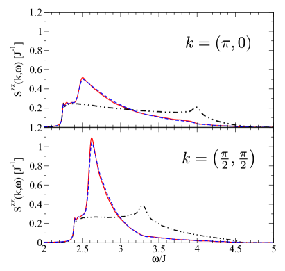
Figure 2: Two-magnon part of the longitudinal dynamic structure factor $S^{zz}({\bf k},\omega)$. Dotted black line: without interaction, dashed blue line: bare interaction, solid red line: renormalized interaction. The curves are computed for $L=192$ using the matrix elements of the $L=16$ system and broadened by $0.013J$. The dispersion is interpolated smoothly, the interaction in a piecewise constant way.

The crucial effects of the magnon-magnon attraction are depicted in Fig. 2 where we computed the longitudinal dynamic structure factor $S^{zz}({\bf k},\omega)$ in the two-magnon $S^{z}_{\text{tot}}=0$ channel without and with (renormalized) interaction. The CST-renormalization of the observable is not included to focus on the pronounced interaction effects. The attraction leads to a shift of spectral weight to lower energies and, strikingly, to the formation of a resonance which we identify as the Higgs resonance. The position of the resonance at $(\pi,0)$ is found to be lower than the one at $(\pi/2,\pi/2)$. This is in line with the argument that the single-magnon dispersion is pushed to lower energies more strongly at $(\pi,0)$ than at $(\pi/2,\pi/2)$ leading to the roton minimum because due to the Higgs resonance the decay of a single magnon not only comprises the decay into three rather independent magnons, but also the decay into two constituents: magnon plus Higgs resonance. In accord with previous studies Schmidt and Uhrig (2005); Fischer et al. (2010, 2011); Fischer (2011); Zhitomirsky and Chernyshev (2013) this is an efficient mechanism to lower the magnon dispersion and to induce the roton minimum.

The renormalization of the interaction in the CST flow enhances the effect of the attraction further. Though this effect is small in absolute terms it makes itself felt in the size of the roton dip. If we switch off the flow of the particle conserving interactions, i.e., without renormalization of the magnon-magnon interaction, the dip of the roton minimum is reduced to $5\%$. This also explains why the third order calculation in $1/S$ yielded only a small dip although some interaction effect was included (diagram (k) in Ref. Syromyatnikov (2010)). Still, the roton minimum is insufficiently captured. Note that the renormalization of the interaction can be as large as $50\%$ for certain momenta sup .

We emphasize that our line shapes in the longitudinal channel agree remarkably well with the experimental data, see Figs. 2c and 2g in Ref. Dalla Piazza et al. (2015). This holds for the position of the Higgs resonances and for the relative heights. Investigating the experimental transverse dynamic structure factor (Figs. 2b and 2f in Ref. Dalla Piazza et al. (2015)) one finds pronounced peaks at $(\pi,0)$ and at $(\pi/2,\pi/2)$. We attribute both of them to magnons and the smaller weight at $(\pi,0)$, combined with a continuum tail, to strong magnon-Higgs scattering. This also shifts the dispersion to lower energies at $(\pi,0)$. Hence, the roton minimum in the magnon dispersion is a fingerprint of the Higgs mode and of strong magnon-Higgs scattering.

Summary — For the $S=1/2$ Heisenberg antiferromagnet on the square lattice, this letter provides a fully consistent and quantitative picture in terms of magnons which describes the low- and the high-energy physics on equal footing. It is achieved by extending the approach of continous unitary transformations to continuous similarity transformations. In momentum space, the flow of the renormalized couplings is closed by the truncation at the level of terms with scaling dimension 2.

The striking agreement of our findings with the experimental results Dalla Piazza et al. (2015) underlines the validity of the magnon quasiparticle picture for long-range ordered quantum magnets at all energies. In this way, the importance of a significant attractive interaction between magnons of different $S^{z}_{\text{tot}}$ is established. This interaction induces a resonance corresponding to the longitudinal magnon or Higgs resonance of the symmetry broken phase. The decay of a magnon into three magnons is strongly enhanced because it is effectively a decay into a magnon and a Higgs resonance. The roton minimum is the fingerprint of this mechanism.

Further studies should address other response functions providing predictions to spectroscopic experiments. We highlight that the developed approach is applicable to a humongous variety of long-range ordered phases. It will help to identify their dynamical properties and eventually their instabilities and ensuing transitions towards other exotic quantum phases.

Supplementary material

This supplementary materials gives all specific informations concerning the extrapolation of the spin wave velocity and the renormalization of the interaction. In addition, details of the CST performed in the main body of the manuscript are given.

.1 Spin wave velocity and magnon-magnon interaction

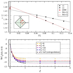
Figure 3: Extrapolation of the results in $1/L$ and comparison to other findings. All lines are linear fits. Upper panel: Spin-wave velocity $v$ deduced from two different directions $v_{1}$ (triangles left) and $v_{2}$ (triangles right) shown in the magnetic Brillioun zone (inset). Lower panel: Renormalization of the attractive interaction of two magnons for smallest, non-zero ${\bf k}$ values along direction $v_{1}$ (see inset upper panel) vs. the flow parameter $\ell$; results for direction $v_{2}$ are almost the same.

Our data for the spin-wave velocity $v$ agrees well with previous results as shown in the upper panel of Fig. 3. It has been determined along two different directions in the BZ yielding $v_{1}$ and $v_{2}$, see upper panel of Fig. 3. Their linearly extrapolated thermodynamic values coincide within the error bar yielding $v/J=1.675\pm 0.025$. This value is in accord with $v^{\rm QMC}/J=1.673\pm 0.007$ from QMC Sandvik (1997).

In the lower panel, we illustrate that the CST procedure renormalizes the interaction sizably. For the smallest non-vanishing momenta the interaction is attractive and renormalized by up to $50\%$. Averaged over all interaction coefficients the renormalization is of the order of $10\%$. Note in addition that not all terms of the interaction act attractively.

.2 Flow equation of the continuous similarity transformation

Below, we give all specific informations concerning the CST performed in the main body of the manuscript: the initial Hamiltonian $\mathcal{H}$ and the initial generator $\eta$, the flowing Hamiltonian $\mathcal{H}(\ell)$ and the flowing generator $\eta(\ell)$ as well as the corresponding flow equations.

.3 Initial Hamiltonian and initial generator

The initial Hamiltonian before the CST is given by

$$\mathcal{H}=E_{0}+\sum_{{\bf k}}\omega_{{\bf k}}(\alpha^{\dagger}_{{\bf k}}\alpha^{\phantom{\dagger}}_{{\bf k}}+\beta^{\dagger}_{{\bf k}}\beta^{\phantom{\dagger}}_{{\bf k}})+\mathcal{V}\,.$$ (4)

The coefficients of the quadratic part are $E_{0}/N=-2J(S^{2}+AS+A^{2}/4)$, $\omega_{{\bf k}}=2J(2S+A)\sqrt{1-\gamma_{{\bf k}}^{2}}$ with $\gamma_{{\bf k}}=(\cos k_{x}+\cos k_{y})/2$, $A:=\frac{2}{N}\sum_{\bf k}(1-\sqrt{1-\gamma_{{\bf k}}^{2}})$. The two-magnon interaction $\mathcal{V}$ is given explicitly by

$$\mathcal{V} = -\frac{J}{N}\sum_{1234}\delta_{G}\left({\bf{1+2-3-4}}\right)\;l_{1}l_{2}l_{3}l_{4}$$ (5)

$$\Big{[}V_{1234}^{(1)}\alpha_{1}^{\dagger}\alpha_{2}^{\dagger}\alpha_{3}^{\phantom{\dagger}}\alpha_{4}^{\phantom{\dagger}}+2V_{1234}^{(2)}\alpha_{1}^{\dagger}\beta_{-2}^{\phantom{\dagger}}\alpha_{3}^{\phantom{\dagger}}\alpha_{4}^{\phantom{\dagger}}+2V_{1234}^{(3)}\alpha_{1}^{\dagger}\alpha_{2}^{\dagger}\beta_{-3}^{\dagger}\alpha_{4}+4V_{1234}^{(4)}\alpha_{1}^{\dagger}\alpha_{3}^{\phantom{\dagger}}\beta_{-4}^{\dagger}\beta_{-2}^{\phantom{\dagger}}$$

$$+ 2V_{1234}^{(5)}\beta_{-4}^{\dagger}\alpha_{3}\beta_{-2}\beta_{-1}^{\phantom{\dagger}}+2V_{1234}^{(6)}\beta_{-4}^{\dagger}\beta_{-3}^{\dagger}\alpha_{2}^{\dagger}\beta_{-1}^{\phantom{\dagger}}+V_{1234}^{(7)}\alpha_{1}^{\dagger}\alpha_{2}^{\dagger}\beta_{-3}^{\dagger}\beta_{-4}^{\dagger}+V_{1234}^{(8)}\beta_{-1}^{\phantom{\dagger}}\beta_{-2}^{\phantom{\dagger}}\alpha_{3}^{\phantom{\dagger}}\alpha_{4}^{\phantom{\dagger}}+V_{1234}^{(9)}\beta_{-4}^{\dagger}\beta_{-3}^{\dagger}\beta_{-2}^{\phantom{\dagger}}\beta_{-1}^{\phantom{\dagger}}\Big{]}\,.\quad$$

The subscripts $i=1,2,3,4$ stand for the momenta ${\bf k}_{i}$ and $-i$ stands for $-{\bf k}_{i}$. The conservation of momentum in the lattice is ensured by the Kronecker symbol $\delta_{G}\left({\bf{k}}\right)$ which implies ${\bf k}=0$ modulo reciprocal lattice vectors from the reciprocal lattice $\Gamma_{A}^{*}$ of the $A$-sites, i.e., ${\bf g}\in\Gamma_{A}^{*}$ means ${\bf g}=(n\pi,m\pi)$ with the integers $n,m$ if the lattice constant of the original square lattice is set to unity. The vertex functions $V_{1234}^{(i)}$ are given explicitly in Ref. Uhrig and Majumdar, 2013.

.4 Flowing Hamiltonian and flowing generator

We include all terms in the flowing Hamiltonian $\mathcal{H}(\ell)$ with a scaling dimension $d\leq 2$. Explicitly, one finds

$$\mathcal{H}(\ell)=E_{0}\ + \sum_{\bf 1} \omega\left({\bf 1}\right)\left(\alpha_{\bf{1}}^{\dagger}\alpha_{\bf{1}}^{\phantom{\dagger}}+\beta_{\bf{1}}^{\dagger}\beta_{\bf{1}}^{\phantom{\dagger}}\right)+\Gamma\left(\bf{1}\right)\left(\alpha_{\bf{1}}^{\dagger}\beta_{\bf{\scalebox{0.5}[1.0]{$-$}1}}^{\dagger}+\alpha_{\bf{1}}^{\phantom{\dagger}}\beta_{\bf{\scalebox{0.5}[1.0]{$-$}1}}^{\phantom{\dagger}}\right)$$

$$+ \sum_{\bf 1,2,3,4} \Bigl{\{}C_{1}\left(\bf{1234}\right)\alpha_{\bf{1}}^{\dagger}\alpha_{\bf{2}}^{\dagger}\alpha_{\bf{3}}^{\phantom{\dagger}}\alpha_{\bf{4}}^{\phantom{\dagger}}+C_{2}\left(\bf{1234}\right)\alpha_{\bf{1}}^{\dagger}\alpha_{\bf{2}}^{\phantom{\dagger}}\beta_{\bf{3}}^{\dagger}\beta_{\bf{4}}^{\phantom{\dagger}}+C_{3}\left(\bf{1234}\right)\beta_{\bf{1}}^{\dagger}\beta_{\bf{2}}^{\dagger}\beta_{\bf{3}}^{\phantom{\dagger}}\beta_{\bf{4}}^{\phantom{\dagger}}\Bigr{.}$$

$$+ C_{4}\left(\bf{1234}\right)\alpha_{\bf{1}}^{\dagger}\alpha_{\bf{2}}^{\dagger}\alpha_{\bf{3}}^{\phantom{\dagger}}\beta_{\bf{4}}^{\dagger}+C_{5}\left(\bf{1234}\right)\alpha_{\bf{1}}^{\dagger}\beta_{\bf{2}}^{\dagger}\beta_{\bf{3}}^{\dagger}\beta_{\bf{4}}^{\phantom{\dagger}}+C_{6}\left(\bf{1234}\right)\alpha_{\bf{1}}^{\dagger}\alpha_{\bf{2}}^{\phantom{\dagger}}\alpha_{\bf{3}}^{\phantom{\dagger}}\beta_{\bf{4}}^{\phantom{\dagger}}$$

. $$+ C_{7}\left(\bf{1234}\right)\alpha_{\bf{1}}^{\phantom{\dagger}}\beta_{\bf{2}}^{\dagger}\beta_{\bf{3}}^{\phantom{\dagger}}\beta_{\bf{4}}^{\phantom{\dagger}}+C_{8}\left(\bf{1234}\right)\alpha_{\bf{1}}^{\dagger}\alpha_{\bf{2}}^{\dagger}\beta_{\bf{3}}^{\dagger}\beta_{\bf{4}}^{\dagger}+C_{9}\left(\bf{1234}\right)\alpha_{\bf{1}}^{\phantom{\dagger}}\alpha_{\bf{2}}^{\phantom{\dagger}}\beta_{\bf{3}}^{\phantom{\dagger}}\beta_{\bf{4}}^{\phantom{\dagger}}\Bigr{\}}\quad.$$ (6)

The corresponding flowing generator is then given by

$$\eta(\ell)= \sum_{\bf 1} \Gamma\left(\bf{1}\right)\left(\alpha_{\bf{1}}^{\dagger}\beta_{\bf{\scalebox{0.5}[1.0]{$-$}1}}^{\dagger}-\alpha_{\bf{1}}^{\phantom{\dagger}}\beta_{\bf{\scalebox{0.5}[1.0]{$-$}1}}^{\phantom{\dagger}}\right)$$

$$+ \sum_{\bf 1,2,3,4} \Bigl{\{}C_{4}\left(\bf{1234}\right)\alpha_{\bf{1}}^{\dagger}\alpha_{\bf{2}}^{\dagger}\alpha_{\bf{3}}^{\phantom{\dagger}}\beta_{\bf{4}}^{\dagger}+C_{5}\left(\bf{1234}\right)\alpha_{\bf{1}}^{\dagger}\beta_{\bf{2}}^{\dagger}\beta_{\bf{3}}^{\dagger}\beta_{\bf{4}}^{\phantom{\dagger}}-C_{6}\left(\bf{1234}\right)\alpha_{\bf{1}}^{\dagger}\alpha_{\bf{2}}^{\phantom{\dagger}}\alpha_{\bf{3}}^{\phantom{\dagger}}\beta_{\bf{4}}^{\phantom{\dagger}}$$

. $$- C_{7}\left(\bf{1234}\right)\alpha_{\bf{1}}^{\phantom{\dagger}}\beta_{\bf{2}}^{\dagger}\beta_{\bf{3}}^{\phantom{\dagger}}\beta_{\bf{4}}^{\phantom{\dagger}}+C_{8}\left(\bf{1234}\right)\alpha_{\bf{1}}^{\dagger}\alpha_{\bf{2}}^{\dagger}\beta_{\bf{3}}^{\dagger}\beta_{\bf{4}}^{\dagger}-C_{9}\left(\bf{1234}\right)\alpha_{\bf{1}}^{\phantom{\dagger}}\alpha_{\bf{2}}^{\phantom{\dagger}}\beta_{\bf{3}}^{\phantom{\dagger}}\beta_{\bf{4}}^{\phantom{\dagger}}\Bigr{\}}\quad.$$ (7)

The coefficients $E_{0}$, $\omega\left({\bf 1}\right)$, $\Gamma\left(\bf{1}\right)$, and $C_{i}\left(\bf{1234}\right)$ depend on the flow parameter $\ell$ and satisfy the initial conditions

$$E_{0}\bigl{|}_{\ell=0} = -2J(S^{2}+AS+A^{2}/4)$$ (8a)

$$\omega\left({\bf 1}\right)\bigl{|}_{\ell=0} = 2J(2S+A)\sqrt{1-\gamma_{\bf 1}^{2}}$$ (8b)

$$\Gamma\left(\bf{1}\right)\bigl{|}_{\ell=0} = 0$$ (8c)

$$C_{1}\left(\bf{1234}\right)\bigl{|}_{\ell=0} = -{l_{1}l_{2}l_{3}l_{4}}\frac{J}{N}V_{1234}^{(1)}\delta_{G}\left({\bf{1+2-3-4}}\right)$$ (8d)

$$C_{2}\left(\bf{1234}\right)\bigl{|}_{\ell=0} = -4{l_{1}l_{2}l_{3}l_{4}}\frac{J}{N}V_{1\scalebox{0.5}[1.0]{$-$}42\scalebox{0.5}[1.0]{$-$}3}^{(4)}\delta_{G}\left({\bf{1-2+3-4}}\right)$$ (8e)

$$C_{3}\left(\bf{1234}\right)\bigl{|}_{\ell=0} = -{l_{1}l_{2}l_{3}l_{4}}\frac{J}{N}V_{\scalebox{0.5}[1.0]{$-$}4\scalebox{0.5}[1.0]{$-$}3\scalebox{0.5}[1.0]{$-$}2\scalebox{0.5}[1.0]{$-$}1}^{(9)}\delta_{G}\left({\bf{1+2-3-4}}\right)$$ (8f)

$$C_{4}\left(\bf{1234}\right)\bigl{|}_{\ell=0} = -2{l_{1}l_{2}l_{3}l_{4}}\frac{J}{N}V_{12\scalebox{0.5}[1.0]{$-$}43}^{(3)}\delta_{G}\left({\bf{1+2-3+4}}\right)$$ (8g)

$$C_{5}\left(\bf{1234}\right)\bigl{|}_{\ell=0} = -2{l_{1}l_{2}l_{3}l_{4}}\frac{J}{N}V_{\scalebox{0.5}[1.0]{$-$}4\scalebox{0.5}[1.0]{$-$}1\scalebox{0.5}[1.0]{$-$}2\scalebox{0.5}[1.0]{$-$}3}^{(6)}\delta_{G}\left({\bf{1+2+3-4}}\right)$$ (8h)

$$C_{6}\left(\bf{1234}\right)\bigl{|}_{\ell=0} = -2{l_{1}l_{2}l_{3}l_{4}}\frac{J}{N}V_{1\scalebox{0.5}[1.0]{$-$}423}^{(2)}\delta_{G}\left({\bf{1-2-3-4}}\right)$$ (8i)

$$C_{7}\left(\bf{1234}\right)\bigl{|}_{\ell=0} = -2{l_{1}l_{2}l_{3}l_{4}}\frac{J}{N}V_{\scalebox{0.5}[1.0]{$-$}4\scalebox{0.5}[1.0]{$-$}31\scalebox{0.5}[1.0]{$-$}2}^{(5)}\delta_{G}\left({\bf{-1+2-3-4}}\right)$$ (8j)

$$C_{8}\left(\bf{1234}\right)\bigl{|}_{\ell=0} = -{l_{1}l_{2}l_{3}l_{4}}\frac{J}{N}V_{12\scalebox{0.5}[1.0]{$-$}3\scalebox{0.5}[1.0]{$-$}4}^{(7)}\delta_{G}\left({\bf{1+2+3+4}}\right)$$ (8k)

$$C_{9}\left(\bf{1234}\right)\bigl{|}_{\ell=0} = -{l_{1}l_{2}l_{3}l_{4}}\frac{J}{N}V_{\scalebox{0.5}[1.0]{$-$}3\scalebox{0.5}[1.0]{$-$}412}^{(8)}\delta_{G}\left({\bf{-1-2-3-4}}\right)\quad.$$ (8l)

Note that the hexatic three-magnon part of the Hamiltonian consisting of six magnon annihilation or creation operators has a scaling dimension $d=4$ and are therefore not relevant at studied level of truncation $d=2$.

.5 Flow equations

Inserting $\mathcal{H}(\ell)$ and $\eta(\ell)$ into the flow equation $\partial_{\ell}\mathcal{H}(\ell)=\left[\eta(\ell),\mathcal{H}(\ell)\right]$ and keeping self-similarly all operators already present in $\mathcal{H}(\ell)$, one obtains the following flow equations

$$\partial_{l}E_{0}= \sum_{\bf 1,23,4} (-8)C_{8}\left(\bf{1234}\right)C_{9}\left(\bf{1234}\right)+\sum_{\bf 1}(-2)\Gamma\left(\bf{1}\right)\Gamma\left(\bf{1}\right)$$ (9a)

$$\partial_{l}\omega\left({\bf 1}\right)=(-2)\Gamma\left(\bf{1}\right)\Gamma\left(\bf{1}\right)+ \sum_{\bf 3,4} \Bigl{\{}-4C_{4}\left(\bf{3415}\right)C_{6}\left(\bf{1345}\right)\delta_{G}\left({\bf{3+4-1+5}}\right)\Bigr{.}$$

$$-16C_{8}\left(\bf{1345}\right)C_{9}\left(\bf{1345}\right)\delta_{G}\left({\bf{3+4+1+5}}\right)$$

. $$-4C_{8}\left(\bf{131{\scalebox{0.5}[1.0]{$-$}3}}\right)\Gamma\left(\bf{3}\right)-4C_{6}\left(\bf{113{\scalebox{0.5}[1.0]{$-$}3}}\right)\Gamma\left(\bf{3}\right)\Bigr{\}}$$ (9b)

$$\partial_{l}\Gamma\left(\bf{1}\right)=-2\Gamma\left(\bf{1}\right)\omega\left({\bf 1}\right)-8 \sum_{3,4,5} \Bigl{\{}C_{4}\left(\bf{3415}\right)C_{9}\left(\bf{34\scalebox{0.5}[1.0]{$-$}15}\right)\delta_{G}\left({\bf{-1+3+4+5}}\right)\Bigr{.}$$ (9c)

$$\Bigl{.}-8C_{5}\left(\bf{345\scalebox{0.5}[1.0]{$-$}1}\right)C_{9}\left(\bf{1345}\right)\delta_{G}\left({\bf{1+3+4+5}}\right)\Bigr{.}$$

$$\sum_{3} \Bigl{\{}C_{2}\left(\bf{13\scalebox{0.5}[1.0]{$-$}1\scalebox{0.5}[1.0]{$-$}3}\right)\Gamma\left(\bf{3}\right)\Bigr{.}$$

$$\Bigl{.}C_{8}\left(\bf{13\scalebox{0.5}[1.0]{$-$}1\scalebox{0.5}[1.0]{$-$}3}\right)\Gamma\left(\bf{3}\right)\Bigr{\}}$$

$$\partial_{l}C_{1}\left(\bf{1234}\right) = \delta_{G}\left({\bf{1+2-3-4}}\right)\Bigl{\{}(-1)C_{4}\left(\bf{1243}\right)\Gamma\left(\bf{3}\right)\Bigr{.}$$

$$(-1)C_{4}\left(\bf{1234}\right)\Gamma\left(\bf{4}\right)$$

$$(-1)C_{6}\left(\bf{2345}\right)\Gamma\left(\bf{1}\right)$$

$$(-1)C_{6}\left(\bf{1345}\right)\Gamma\left(\bf{2}\right)$$

$$\sum_{\bf 5,6} (-4)C_{4}\left(\bf{2546}\right)C_{6}\left(\bf{1356}\right)\delta_{G}\left({\bf{2+5-4+6}}\right)$$

$$(-4)C_{4}\left(\bf{1536}\right)C_{6}\left(\bf{2456}\right)\delta_{G}\left({\bf{1+5-3+6}}\right)$$

$$\Bigl{.}(-4)C_{8}\left(\bf{1256}\right)C_{9}\left(\bf{3456}\right)\delta_{G}\left({\bf{1+2+5+6}}\right)\Bigr{\}}$$

$$\partial_{l}C_{2}\left(\bf{1234}\right) = \delta_{G}\left({\bf{1-2+3-4}}\right)\Bigl{\{}(-1)C_{4}\left(\bf{1\scalebox{0.5}[1.0]{$-$}423}\right)\Gamma\left(\bf{\scalebox{0.5}[1.0]{$-$}4}\right)\Bigr{.}$$ (10b)

$$(-1)C_{5}\left(\bf{13\scalebox{0.5}[1.0]{$-$}24}\right)\Gamma\left(\bf{\scalebox{0.5}[1.0]{$-$}2}\right)$$

$$(-1)C_{6}\left(\bf{12\scalebox{0.5}[1.0]{$-$}34}\right)\Gamma\left(\bf{\scalebox{0.5}[1.0]{$-$}3}\right)$$

$$(-1)C_{7}\left(\bf{234\scalebox{0.5}[1.0]{$-$}1}\right)\Gamma\left(\bf{\scalebox{0.5}[1.0]{$-$}1}\right)$$

$$\sum_{\bf 5,6} (-4)C_{4}\left(\bf{5623}\right)C_{6}\left(\bf{1564}\right)\delta_{G}\left({\bf{5+6-2+3}}\right)$$

$$(-4)C_{5}\left(\bf{1564}\right)C_{7}\left(\bf{2356}\right)\delta_{G}\left({\bf{1+5+6-4}}\right)$$

$$(-8)C_{4}\left(\bf{1526}\right)C_{6}\left(\bf{5346}\right)\delta_{G}\left({\bf{1+5-2+6}}\right)$$

$$(-8)C_{5}\left(\bf{5364}\right)C_{7}\left(\bf{1256}\right)\delta_{G}\left({\bf{5+3+6-4}}\right)$$

$$\Bigl{.}(-32)C_{8}\left(\bf{1536}\right)C_{9}\left(\bf{2546}\right)\delta_{G}\left({\bf{1+5+3+6}}\right)\Bigr{\}}$$

$$\partial_{l}C_{3}\left(\bf{1234}\right) = \delta_{G}\left({\bf{1+2-3-4}}\right)\Bigl{\{}(-1)C_{5}\left(\bf{{\scalebox{0.5}[1.0]{$-$}3}124}\right)\Gamma\left(\bf{\scalebox{0.5}[1.0]{$-$}3}\right)\Bigr{.}$$ (10c)

$$(-1)C_{5}\left(\bf{\scalebox{0.5}[1.0]{$-$}4123}\right)\Gamma\left(\bf{\scalebox{0.5}[1.0]{$-$}4}\right)$$

$$(-1)C_{7}\left(\bf{\scalebox{0.5}[1.0]{$-$}2134}\right)\Gamma\left(\bf{\scalebox{0.5}[1.0]{$-$}2}\right)$$

$$(-1)C_{7}\left(\bf{{\scalebox{0.5}[1.0]{$-$}1}234}\right)\Gamma\left(\bf{\scalebox{0.5}[1.0]{$-$}1}\right)$$

$$\sum_{\bf 5} (-4)C_{5}\left(\bf{5264}\right)C_{7}\left(\bf{5136}\right)\delta_{G}\left({\bf{5+1+6-4}}\right)$$

$$(-4)C_{5}\left(\bf{5163}\right)C_{7}\left(\bf{5246}\right)\delta_{G}\left({\bf{5+1+6-3}}\right)$$

$$\Bigl{.}(-4)C_{8}\left(\bf{5612}\right)C_{9}\left(\bf{5634}\right)\delta_{G}\left({\bf{5+6+1+2}}\right)\Bigr{\}}$$

$$\partial_{l}C_{4}\left(\bf{1234}\right) = \delta_{G}\left({\bf{1+2-3+4}}\right)\Bigl{\{}\left(\omega\left({\bf 3}\right)-\omega\left({\bf 1}\right)-\omega\left({\bf 2}\right)-\omega\left({\bf 4}\right)\right)C_{4}\left(\bf{1234}\right)\Bigr{.}$$ (10d)

$$(-2)C_{1}\left(\bf{123\scalebox{0.5}[1.0]{$-$}4}\right)\Gamma\left(\bf{\scalebox{0.5}[1.0]{$-$}4}\right)$$

$$\left(-\frac{1}{2}\right)\left(C_{2}\left(\bf{234\scalebox{0.5}[1.0]{$-$}1}\right)\Gamma\left(\bf{1}\right)+C_{2}\left(\bf{134\scalebox{0.5}[1.0]{$-$}2}\right)\Gamma\left(\bf{2}\right)\right)$$

$$(-4)C_{8}\left(\bf{124\scalebox{0.5}[1.0]{$-$}3}\right)\Gamma\left(\bf{3}\right)$$

$$\sum_{\bf 5,6} (-2)C_{1}\left(\bf{1256}\right)C_{4}\left(\bf{5634}\right)\delta_{G}\left({\bf{1+2-5-6}}\right)$$

$$(-1)C_{2}\left(\bf{2546}\right)C_{4}\left(\bf{1536}\right)\delta_{G}\left({\bf{2-5+4-6}}\right)$$

$$(-1)C_{2}\left(\bf{1546}\right)C_{4}\left(\bf{2536}\right)\delta_{G}\left({\bf{1-5+4-6}}\right)$$

$$(-8)C_{6}\left(\bf{2356}\right)C_{8}\left(\bf{1546}\right)\delta_{G}\left({\bf{2-3-5-6}}\right)$$

$$(-8)C_{6}\left(\bf{1356}\right)C_{8}\left(\bf{2546}\right)\delta_{G}\left({\bf{1-3-5-6}}\right)$$

$$\Bigl{.}(-4)C_{7}\left(\bf{3456}\right)C_{8}\left(\bf{1256}\right)\delta_{G}\left({\bf{3-4+5+6}}\right)\Bigr{\}}$$

$$\partial_{l}C_{5}\left(\bf{1234}\right) = \delta_{G}\left({\bf{1+2+3-4}}\right)\Bigl{\{}\left(-\omega\left({\bf 1}\right)-\omega\left({\bf 2}\right)-\omega\left({\bf 3}\right)+\omega\left({\bf 4}\right)\right)C_{5}\left(\bf{1234}\right)\Bigr{.}$$ (10e)

$$(-2)C_{3}\left(\bf{234\scalebox{0.5}[1.0]{$-$}1}\right)\Gamma\left(\bf{1}\right)$$

$$\left(-\frac{1}{2}\right)\left(C_{2}\left(\bf{1\scalebox{0.5}[1.0]{$-$}234}\right)\Gamma\left(\bf{\scalebox{0.5}[1.0]{$-$}2}\right)+C_{2}\left(\bf{1\scalebox{0.5}[1.0]{$-$}324}\right)\Gamma\left(\bf{\scalebox{0.5}[1.0]{$-$}3}\right)\right)$$

$$(-4)C_{8}\left(\bf{1\scalebox{0.5}[1.0]{$-$}423}\right)\Gamma\left(\bf{\scalebox{0.5}[1.0]{$-$}4}\right)$$

$$\sum_{\bf 5,6} (-2)C_{1}\left(\bf{5623}\right)C_{6}\left(\bf{1564}\right)\delta_{G}\left({\bf{5+6-2-3}}\right)$$

$$(-1)C_{2}\left(\bf{1536}\right)C_{5}\left(\bf{5264}\right)\delta_{G}\left({\bf{1-5+3-6}}\right)$$

$$(-1)C_{2}\left(\bf{1526}\right)C_{5}\left(\bf{5364}\right)\delta_{G}\left({\bf{1-5+2-6}}\right)$$

$$(-8)C_{7}\left(\bf{5346}\right)C_{8}\left(\bf{1526}\right)\delta_{G}\left({\bf{5-3+4+6}}\right)$$

$$(-8)C_{7}\left(\bf{5246}\right)C_{8}\left(\bf{1536}\right)\delta_{G}\left({\bf{5-2+4+6}}\right)$$

$$\Bigl{.}(-4)C_{6}\left(\bf{1564}\right)C_{8}\left(\bf{5623}\right)\delta_{G}\left({\bf{1-5-6-4}}\right)\Bigr{\}}$$

$$\partial_{l}C_{6}\left(\bf{1234}\right) = \delta_{G}\left({\bf{1-2-3-4}}\right)\Bigl{\{}\left(\omega\left({\bf 1}\right)-\omega\left({\bf 2}\right)-\omega\left({\bf 3}\right)-\omega\left({\bf 4}\right)\right)C_{6}\left(\bf{1234}\right)\Bigr{.}$$ (10f)

$$(-2)C_{1}\left(\bf{1\scalebox{0.5}[1.0]{$-$}423}\right)\Gamma\left(\bf{\scalebox{0.5}[1.0]{$-$}4}\right)$$

$$\left(-\frac{1}{2}\right)\left(C_{2}\left(\bf{13\scalebox{0.5}[1.0]{$-$}24}\right)\Gamma\left(\bf{2}\right)+C_{2}\left(\bf{12\scalebox{0.5}[1.0]{$-$}24}\right)\Gamma\left(\bf{3}\right)\right)$$

$$(-4)C_{9}\left(\bf{234\scalebox{0.5}[1.0]{$-$}1}\right)\Gamma\left(\bf{1}\right)$$

$$\sum_{\bf 5,6} (-2)C_{1}\left(\bf{5623}\right)C_{6}\left(\bf{1564}\right)\delta_{G}\left({\bf{5+6-2-3}}\right)$$

$$(-1)C_{2}\left(\bf{5364}\right)C_{6}\left(\bf{1256}\right)\delta_{G}\left({\bf{5-3+6-4}}\right)$$

$$(-1)C_{2}\left(\bf{5264}\right)C_{6}\left(\bf{1356}\right)\delta_{G}\left({\bf{5-2+6-4}}\right)$$

$$(-8)C_{4}\left(\bf{1536}\right)C_{9}\left(\bf{2546}\right)\delta_{G}\left({\bf{1+5-3+6}}\right)$$

$$(-8)C_{4}\left(\bf{1526}\right)C_{9}\left(\bf{3546}\right)\delta_{G}\left({\bf{1+5-2+6}}\right)$$

$$\Bigl{.}(-4)C_{5}\left(\bf{1564}\right)C_{9}\left(\bf{2356}\right)\delta_{G}\left({\bf{1+5+6-4}}\right)\Bigr{\}}$$

$$\partial_{l}C_{7}\left(\bf{1234}\right) = \delta_{G}\left({\bf{1-2+3+4}}\right)\Bigl{\{}\left(-\omega\left({\bf 1}\right)+\omega\left({\bf 2}\right)-\omega\left({\bf 3}\right)-\omega\left({\bf 4}\right)\right)C_{7}\left(\bf{1234}\right)\Bigr{.}$$ (10g)

$$(-2)C_{3}\left(\bf{2\scalebox{0.5}[1.0]{$-$}134}\right)\Gamma\left(\bf{1}\right)$$

$$\left(-\frac{1}{2}\right)\left(C_{2}\left(\bf{\scalebox{0.5}[1.0]{$-$}3124}\right)\Gamma\left(\bf{\scalebox{0.5}[1.0]{$-$}3}\right)+C_{2}\left(\bf{\scalebox{0.5}[1.0]{$-$}4123}\right)\Gamma\left(\bf{\scalebox{0.5}[1.0]{$-$}4}\right)\right)$$

$$(-4)C_{9}\left(\bf{1\scalebox{0.5}[1.0]{$-$}234}\right)\Gamma\left(\bf{\scalebox{0.5}[1.0]{$-$}2}\right)$$

$$\sum_{\bf 5,6} (-2)C_{3}\left(\bf{5634}\right)C_{7}\left(\bf{1256}\right)\delta_{G}\left({\bf{5+6-3-4}}\right)+$$

$$(-1)C_{2}\left(\bf{5164}\right)C_{7}\left(\bf{5236}\right)\delta_{G}\left({\bf{5-1+6-4}}\right)$$

$$(-1)C_{2}\left(\bf{5163}\right)C_{7}\left(\bf{5246}\right)\delta_{G}\left({\bf{5-1+6-3}}\right)$$

$$(-8)C_{5}\left(\bf{5264}\right)C_{9}\left(\bf{1536}\right)\delta_{G}\left({\bf{5+2+6-4}}\right)$$

$$(-8)C_{5}\left(\bf{5263}\right)C_{9}\left(\bf{1546}\right)\delta_{G}\left({\bf{5+2+6-3}}\right)$$

$$\Bigl{.}(-4)C_{4}\left(\bf{5612}\right)C_{9}\left(\bf{5634}\right)\delta_{G}\left({\bf{5+6-1+2}}\right)\Bigr{\}}$$

$$\partial_{l}C_{8}\left(\bf{1234}\right) = \delta_{G}\left({\bf{1+2+3+4}}\right)\Bigl{\{}\left(-\omega\left({\bf 1}\right)-\omega\left({\bf 2}\right)-\omega\left({\bf 3}\right)-\omega\left({\bf 4}\right)\right)C_{8}\left(\bf{1234}\right)\Bigr{.}$$ (10h)

$$\sum_{\bf 5,6} (-2)C_{1}\left(\bf{1256}\right)C_{8}\left(\bf{5634}\right)\delta_{G}\left({\bf{1+2-5-6}}\right)$$

$$(-1)C_{2}\left(\bf{2546}\right)C_{8}\left(\bf{1536}\right)\delta_{G}\left({\bf{2-5+4-6}}\right)$$

$$(-1)C_{2}\left(\bf{1546}\right)C_{8}\left(\bf{2536}\right)\delta_{G}\left({\bf{1-5+4-6}}\right)$$

$$(-1)C_{2}\left(\bf{2536}\right)C_{8}\left(\bf{1546}\right)\delta_{G}\left({\bf{2-5+3-6}}\right)$$

$$(-1)C_{2}\left(\bf{1536}\right)C_{8}\left(\bf{2546}\right)\delta_{G}\left({\bf{1-5+3-6}}\right)$$

$$\Bigl{.}(-2)C_{3}\left(\bf{3456}\right)C_{8}\left(\bf{1256}\right)\delta_{G}\left({\bf{3+4-5-6}}\right)\Bigr{\}}$$

$$\partial_{l}C_{9}\left(\bf{1234}\right) = \delta_{G}\left({\bf{1+2+3+4}}\right)\Bigl{\{}\left(-\omega\left({\bf 1}\right)-\omega\left({\bf 2}\right)-\omega\left({\bf 3}\right)-\omega\left({\bf 4}\right)\right)C_{9}\left(\bf{1234}\right)\Bigr{.}$$ (10i)

$$\sum_{\bf 5,6} (-2)(-2)C_{1}\left(\bf{5612}\right)C_{9}\left(\bf{5634}\right)\delta_{G}\left({\bf{5+6-1-2}}\right)$$

$$(-1)C_{2}\left(\bf{5264}\right)C_{9}\left(\bf{1536}\right)\delta_{G}\left({\bf{5-2+6-4}}\right)$$

$$(-1)C_{2}\left(\bf{5164}\right)C_{9}\left(\bf{2536}\right)\delta_{G}\left({\bf{5-1+6-4}}\right)$$

$$(-1)C_{2}\left(\bf{5263}\right)C_{9}\left(\bf{1546}\right)\delta_{G}\left({\bf{5-2+6-3}}\right)$$

$$(-1)C_{2}\left(\bf{5163}\right)C_{9}\left(\bf{2546}\right)\delta_{G}\left({\bf{5-1+6-3}}\right)$$

$$\Bigl{.}(-2)C_{3}\left(\bf{5634}\right)C_{9}\left(\bf{1256}\right)\delta_{G}\left({\bf{3+4-5-6}}\right)\Bigr{\}}$$

Note that the Kronecker symbols $\delta_{G}\left({\bf{k}}\right)$ in the sums are redundant since the coefficients intrinsically conserve the total momentum by definition (see Eq. (8)). They are included to underline momentum conservation.

References

Laughlin (1983)R. B. Laughlin, Phys. Rev. Lett. 50, 1395 (1983).
Castelnovo et al. (2008)C. Castelnovo, R. Moessner, and S. L. Sondhi, Nature 451, 42
(2008).
Anderson (1987)P. W. Anderson, Science 235, 1196
(1987).
Knetter et al. (2001)C. Knetter, K. P. Schmidt, M. Grüninger, and G. S. Uhrig, Phys.
Rev. Lett. 87, 167204
(2001).
Reger and Young (1988)J. D. Reger and A. P. Young, Phys.
Rev. B 37, 5978
(1988).
Chakravarty et al. (1989)S. Chakravarty, B. I. Halperin, and D. R. Nelson, Phys.
Rev. B 39, 2344
(1989).
Auerbach (1994)A. Auerbach, Interacting Electrons
and Quantum Magnetism, Graduate Texts in Contemporary Physics (Springer, New York, 1994).
Christensen et al. (2007)N. B. Christensen, H. M. Rønnow, D. F. McMorrow, A. Harrison,
T. G. Perring, M. Enderle, R. Coldea, L. P. Regnault, and G. Aeppli, Proc. Nat. Acad. Sciences 104, 15264 (2007).
Dalla Piazzaet al. (2015)B. Dalla Piazza, M. Mourigal, N. B. Christensen, G. J. Nilsen, P. Tregenna-Piggott, T. G. Perring, M. Enderle,
D. F. McMorrow, D. A. Ivanov, and H. M. Rønnow, Nature Phys. 11, 62 (2015).
Le Tacon et al. (2011)M. Le Tacon, G. Ghiringhelli, J. Chaloupka, M. M. Sala,
V. Hinkov, M. Haverkort, M. Minola, M. Bakr, K. J. Zhou, S. Blanco-Canosa, C. Monney, Y. T. Song,
G. L. Sun, C. T. Lin, G. M. D. Luca, M. Salluzzo, G. Khaliullin, T. Schmitt, L. Braicovic, and B. Keimer, Nature Phys. 7, 725 (2011).
Hamer et al. (1992)C. J. Hamer, W. Zheng, and P. Arndt, Phys. Rev. B 46, 6276 (1992).
Weihong and Hamer (1993)Z. Weihong and C. J. Hamer, Phys.
Rev. B 47, 7961
(1993).
Igarashi and Nagao (2005)J. Igarashi and T. Nagao, Phys.
Rev. B 72, 014403
(2005).
Syromyatnikov (2010)A. V. Syromyatnikov, J. Phys. C 22, 216003
(2010).
Uhrig and Majumdar (2013)G. S. Uhrig and K. Majumdar, Eur.
Phys. J. B 86, 282
(2013).
Sandvik and Singh (2001)A. W. Sandvik and R. R. P. Singh, Phys.
Rev. Lett. 86, 528
(2001).
Zheng et al. (2005)W. Zheng, J. Oitmaa, and C. J. Hamer, Phys. Rev. B 71, 184440 (2005).
Vollhardt and Wölfle (1990)D. Vollhardt and P. Wölfle, The Superfluid Phases
of Helium 3 (Taylor and Francis, London, 1990).
Ch.-M.Ho et al. (2001)Ch.-M.Ho, V. N. Muthukumar, M. Ogata, and P. W. Anderson, Phys. Rev. Lett. 86, 1626 (2001).
Tang and Sandvik (2013)Y. Tang and A. W. Sandvik, Phys.
Rev. Lett. 110, 217213
(2013).
Schmidt and Uhrig (2003)K. P. Schmidt and G. S. Uhrig, Phys.
Rev. Lett. 90, 227204
(2003).
Faddeev and Takhtajan (1981)L. D. Faddeev and L. A. Takhtajan, Phys. Lett. 85A, 375
(1981).
Lake et al. (2000)B. Lake, D. A. Tennant, and S. E. Nagler, Phys. Rev. Lett. 85, 832 (2000).
Rüegg et al. (2008)C. Rüegg, B. Normand,
M. Matsumoto, A. Furrer, D. F. McMorrow, K. W. Krämer, H. U. Güdel, S. N. Gvasaliya, H. Mutka, and M. Boehm, Phys. Rev. Lett. 100, 205701 (2008).
Pekker and Varma (2015)D. Pekker and C. M. Varma, Annual
Review of Condensed Matter Physics 6, 269 (2015).
Dyson (1956)F. J. Dyson, Phys.
Rev. 102, 1217 (1956).
Wegner (1994) F. Wegner, Ann. Physik 3, 77 (1994).
Knetter and Uhrig (2000)C. Knetter and G. S. Uhrig, Eur.
Phys. J. B 13, 209
(2000).
Fischer et al. (2010)T. Fischer, S. Duffe, and G. S. Uhrig, New J. Phys. 10, 033048 (2010).
Knetter et al. (2003)C. Knetter, K. P. Schmidt, and G. S. Uhrig, J.
Phys. A: Math. Gen. 36, 7889 (2003).
Kehrein (2006)S. Kehrein, The Flow Equation
Approach to Many-Particle Systems, Springer Tracts in
Modern Physics, Vol. 217 (Springer, Berlin, 2006).
Krull et al. (2012)H. Krull, N. A. Drescher,
and G. S. Uhrig, Phys. Rev. B 86, 125113 (2012).
Yang and Schmidt (2011)H.-Y. Yang and K. P. Schmidt, Europhys. Lett. 94, 17004 (2011).
Kehrein (1999)S. Kehrein, Phys.
Rev. Lett. 83, 4914
(1999).
Kehrein (2001)S. Kehrein, Nucl.
Phys. B 592, 512
(2001).
Note (1)For the scaling one must consider the thermodynamic limit
with continuous momenta as in (3\@@italiccorr). The actual calculations are done with discrete momenta.
Sandvik (1997)A. W. Sandvik, Phys.
Rev. B 56, 11678
(1997).
Zhitomirsky and Chernyshev (2013)M. E. Zhitomirsky and A. L. Chernyshev, Rev. Mod. Phys. 85, 219
(2013).
Schmidt and Uhrig (2005)K. P. Schmidt and G. S. Uhrig, Mod.
Phys. Lett. B 19, 1179
(2005).
Fischer et al. (2011)T. Fischer, S. Duffe, and G. S. Uhrig, Europhys. Lett. 96, 47001 (2011).
Fischer (2011)T. Fischer, Description of
quasiparticle decay by continuous unitary transformations (PhD Thesis, available at
t1.physik.uni-dortmund.de/uhrig/phd.html, TU
Dortmund, 2011).