Compressive Rate Estimation with Applications to Device-to-Device Communications

Abstract

We develop a framework that we call compressive rate estimation. We assume that the composite channel gain matrix (i.e. the matrix of all channel gains between all network nodes) is compressible which means it can be approximated by a sparse or low rank representation. We develop and study a novel sensing and reconstruction protocol for the estimation of achievable rates. We develop a sensing protocol that exploits the superposition principle of the wireless channel and enables the receiving nodes to obtain non-adaptive random measurements of columns of the composite channel matrix. The random measurements are fed back to a central controller that decodes the composite channel gain matrix (or parts of it) and estimates individual user rates. We analyze the rate loss for a linear and a non-linear decoder and find the scaling laws according to the number of non-adaptive measurements. In particular, if we consider a system with $N$ nodes and assume that each column of the composite channel matrix is $k$ sparse, our findings can be summarized as follows. For a certain class of non-linear decoders we show that if the number of pilot signals $M$ scales like $M\sim k\log(N/k)$, then the rate loss compared to perfect channel state information remains bounded. For a certain class of linear decoders we show that the rate loss compared to perfect channel state information scales like $1/\sqrt{M}$.

I Introduction

Device-to-device (D2D) communication has evolved as one of the key technology enablers for 5G wireless systems (“Beyond 2020 Networks”) [1]. The basic idea of D2D communication is to establish direct short-distance communication links between pairs of suitably selected wireless devices so that there is no need for long-distance transmissions to and from base stations (BS). Exploiting direct communication between nearby devices has a huge potential for boosting the performance of cellular networks [2] and improving the service quality of proximity based applications [3]. In addition, D2D communication makes some new exciting location-based services and applications possible.

The main potential advantages of D2D communications stem from the proximity-, reuse-, and hop gains that can be summarized as follows [4]:

• Coverage improves since direct D2D links can be used to fill coverage holes;

• Capacity enhances due to the reuse of radio resources of the supporting cellular layer by multiple D2D links [5];

• Energy efficiency increases since transmit powers can be reduced without deteriorating the capacity [6];

• Achievable peak rates increase and end-to-end latencies decrease due to proximity and hop gains.

D2D communication has been extensively studied in the context of ad-hoc networks, in which wireless devices utilize unlicensed spectrum resources with no or strictly limited assistance from a fixed network infrastructure. Such solutions are not suitable for general purpose wireless applications due to the lack of quality-of-service (QoS) guarantees to D2D links [7]. This is also true in the case of other approaches to D2D communication that are based on the concept of cognitive radio and dynamic/opportunistic spectrum access [8]. Therefore, these approaches have found limited acceptance in the standardization bodies.

In order to overcome the limits of unassisted ad-hoc networking technologies and opportunistic spectrum access technologies based on spectrum sensing, researchers have recently turned their attention towards network-assisted D2D communication, which promises more efficient spectrum utilization, QoS support and higher reliability, while providing D2D discovery support, synchronization and security [2, 4, 5]. In particular, the design aspects of D2D communication are currently discussed in 3GPP, where the feasibility and the architecture enhancements of so called proximity services (ProSe) are under discussion [9], [10]. Thereby, D2D links can operate in in-band mode and out-band mode. While the in-band D2D mode utilizes the same spectral resources as cellular users that transmit their data via base stations in the traditional cellular mode, the out-band D2D mode allocates cellular users and D2D links to different frequency bands. We focus on in-band D2D communication and assume that all users are in-coverage, which means that each user is connected to some base station. As an underlay to cellular networks, in-band D2D communication can be seen as a network-assisted interference channel, in which D2D transmissions reuse cellular resources while being assisted by base stations.

Despite key advantages, network-assisted D2D communication also poses some fundamental challenges including transmission mode selection, robust interference management and feedback design. The underlying problems are aggravated by the lack of channel state information (CSI) at different locations in a network. There is in particular a vital need for timely and accurate CSI that can be used by the network controller to facilitate reliable D2D discovery and QoS-aware scheduling. In other words, when establishing D2D links and allocating cellular resources to them, the network controller should have enough CSI to ensure that the QoS demands of all cellular and D2D users (e.g. expressed in terms of some minimum data rate requirements) are guaranteed once in-band D2D links are established. While being highly valuable, CSI is not for free and must be obtained as efficient as possible without consuming to much scarce radio resources. In [11] the authors used methods from compressed sensing to acquire channel state information at the central controller of two-hop network.

I-A Our Contribution

This paper contributes towards the development of measurement-based feedback protocols, with the goal of enabling a network controller to acquire the required CSI in a highly efficient way. Such protocols need to perform the following steps [12]:

• Spectral resource management: The BS assigns cellular users to the available spectral resources. This step is performed in any cellular network with centralized resource management, e.g., 3GPP LTE.

• D2D discovery and mode selection: The BS detects wireless devices that are in proximity to each other (D2D discovery) and decides if a device should operate in cellular mode or D2D mode (mode selection).

• Pairing: The network controller decides if one or more D2D links share a spectral resource with some cellular user.

The focus of this paper is on D2D discovery – also called proximity discovery – and on pairing, which is a part of scheduling decisions that assign resources to cellular users and D2D links. Both tasks – D2D discovery and pairing – are entirely carried out by a network controller where enough CSI is needed for robust decisions. Assuming D2D communication as an underlay to a cellular network, we address the problem of reliable D2D discovery and pairing based on compressed and quantized channel measurements. We develop and study a novel sensing and reconstruction strategy (protocol) for the estimation of achievable rates, which we call compressive rate estimation. The proposed protocol combines the estimation from compressed measurements with coded access to reduce the number of pilot-based measurements that need to be fed back to estimate the achievable rates and to make timely and robust QoS-aware decisions. By using the concept of coded access we are able to exploit collisions in an interference channel to obtain compressed non-adaptive measurements from linear random projections (e.g. analog coding of [13] can be used for this purpose). To estimate the rates, we apply methods from compressed sensing and sparse approximation [14]. Since a major drawback of compressed sensing based techniques is that they require highly complex decoders, we also consider linear estimation methods which require significantly less complexity [15]. As we will see, the advantages of the proposed protocol are three-fold. First, by applying the concept of coded access, we are able to significantly reduce the pilot contamination in the network. Second, the feedback overhead is reduced since significantly fewer measurements need to be quantized and fed back. Third, most of the complexity required to estimate the achievable rates is imposed on the network controller.

I-B Notation

The element in the $i$-th row and $j$-th column of a matrix $\boldsymbol{X}$ is given by $[\boldsymbol{X}]_{i,j}=x_{i,j}$, similarly, the $i$-th element of a vector $\boldsymbol{x}$ is given by $x_{i}$. The conjugate transpose of a matrix $\boldsymbol{X}$ is $\boldsymbol{X}^{H}$. For vectors the $\ell_{p}$–norm is given by $\|\boldsymbol{x}\|_{\ell_{p}}=\left(\sum_{i}\boldsymbol{x}_{i}^{p}\right)^{1/p},p\geq 1$. For matrices the Schatten-$p$ norm is given by $\|\boldsymbol{X}\|_{s_{p}}=\left(\sum_{i}\sigma_{i}^{p}(\boldsymbol{X})\right)^{1/p}$ where $\{\sigma_{i}(\boldsymbol{X})\}_{i}$ are the singular values of the matrix $\boldsymbol{X}$ in decreasing order. The operator $\boldsymbol{x}=\text{vec}(\boldsymbol{X})$ stacks the columns of the matrix $\boldsymbol{X}$ in a large column vector $\boldsymbol{x}$. The support $\text{supp}(\boldsymbol{x})$ of a vector $\boldsymbol{x}$ is the index set of its non-zero elements. The $N\times N$ identity matrix is denoted as $\boldsymbol{I}_{N}$ and its $i$-th column is defined as $\boldsymbol{e}_{i}$. Tuples are denoted by calligraphic letters and the $i$-th element of tuple $\mathcal{X}$ is given by $\mathcal{X}_{i}$. The real numbers are defined as $\mathbb{R}$ and the complex number are $\mathbb{C}$.

II System Model

We consider a cellular network with a large number of wireless devices and multiple base stations that are controlled by a (central) network controller. We assume there are $N>1$ transmitters that wish to establish communication links over the (wireless) channel to transfer independent data to $N$ receivers. Communication links between the wireless devices and the base stations are referred to as cellular users, while the term D2D user or, equivalently, D2D link is used to refer to a communication link between two wireless devices. The users as well as the corresponding transmitters and receivers are indexed in an arbitrary but fixed order with indices taken from the set $\mathcal{N}=\{1,2,\ldots N\}$. A subset $\mathcal{N}_{1}\subseteq\mathcal{N}$ is used to denote cellular users so that the remaining users with indices in $\mathcal{N}\setminus\mathcal{N}_{1}$ are potential D2D users. The cellular users are assumed to have been scheduled for (cellular) transmissions in the downlink channel.

A frequency-division multiple access (FDMA) technique such as OFDMA (OFDMA: orthogonal frequency-division multiple access) together with a time-division multiple access (TDMA) technique is used to divide the available bandwidth and time in a number of mutually orthogonal time-frequency resource units referred to as resource blocks. We assume that the bandwidth and the duration of each resource block are smaller than the coherence bandwidth and the coherence time of the channel, respectively. This implies that the channel for each resource block and each user can be considered to be frequency flat and constant. More precisely, the channel from the transmitter of user $j$ (referred to as transmitter $j$) to the receiver of user $i$ (called receiver $i$) on resource block $(t,f)$ is described by the channel coefficient $h_{i,j}(t,f)\in\mathbb{C}$, which is a realization of some stochastic process. We assume that all resource blocks are statistically equivalent and independent. Therefore, we can consider an arbitrary but fixed resource block and drop the time and frequency index for simplicity.

Given a resource block, user $i\in\mathcal{N}$ may experience interference from other users $j\in\mathcal{N},j\neq i$. As a result, the performance of user $i\in\mathcal{N}$ depends in general on the vector $\boldsymbol{h}_{i}:=\left(h_{i,1},\ldots,h_{i,N}\right)^{T}\in\mathbb{C}^{N}$ of channel coefficients $h_{i,j}\in\mathbb{C}$ from all transmitters $j\in\mathcal{N}$ to receiver $i\in\mathcal{N}$. These channel vectors are grouped in the channel matrix $\boldsymbol{H}:=\left(\boldsymbol{h}_{1},\ldots,\boldsymbol{h}_{N}\right)$ which contains all channel coefficients.

As discussed before, not all potential D2D users in $\mathcal{N}\setminus\mathcal{N}_{1}$ need to be scheduled for transmissions. Therefore, we define $\mathcal{S}\subseteq\mathcal{N}$ to be the index set of users (cellular and D2D) scheduled for transmissions. The signal observed by receiver $i\in\mathcal{S}$ is then

$$y_{i}=h_{i,i}s_{i}+\sum_{j\in\mathcal{S}\setminus\{i\}}h_{i,j}s_{j}+n_{i},$$ (1)

where $s_{j}\in\mathbb{C}$ is the complex data symbol transmitted by node $j$ and $n_{i}\sim\mathcal{C}\mathcal{N}(0,\sigma^{2}_{i})$ is additive noise at receiver $i$. The transmitted data symbols are assumed to be i.i.d. random variables with $\mathbb{E}\left[{s_{j}}\right]=0$ and $\mathbb{E}\left[{|s_{j}|^{2}}\right]=p_{j}$, where the transmit power $p_{j}$ of user $j$ is assumed to be fixed (i.e. we consider no power control). If user $i$ is scheduled for transmission, then its achievable rate is assumed to be

$$r(\boldsymbol{h}_{i},\mathcal{S})=\log\bigl{(}1+\text{SINR}(\boldsymbol{h}_{i},\mathcal{S})\bigr{)}$$ (2)

where the SINR of receiver $i\in\mathcal{S}$ is defined as the ratio of the desired signal power to the sum of the interference and noise power:

$$\text{SINR}(\boldsymbol{h}_{i},\mathcal{S}):=\frac{p_{i}|h_{i,i}|^{2}}{\sigma^{2}_{i}+\sum_{j\in\mathcal{S}\setminus\{i\}}p_{j}|h_{i,j}|^{2}}.$$ (3)

In what follows, we assume that each receiver $i$ has a rate (or quality-of-service) requirement $\bar{r}_{i}$ and we define a feasible scheduling decision as follows.

Definition 1 (Feasible scheduling decision).

Given a channel matrix $\boldsymbol{H}$, we say that a scheduling decision $\mathcal{S}$ is feasible if $\mathcal{N}_{1}\subseteq\mathcal{S}$ and $r(\boldsymbol{h}_{i},\mathcal{S})\geq\bar{r}_{i}$ holds for each $i\in\mathcal{S}\subseteq\mathcal{N}.$

We emphasize that by the definition, $r(\boldsymbol{h}_{i},\mathcal{S})\geq\bar{r}_{i}$ for each $i\in\mathcal{N}_{1}\subseteq\mathcal{S}$ whenever $\mathcal{S}$ is feasible. In other words, the requirements of cellular users are satisfied per definition and $\mathcal{N}_{1}$ is a feasible scheduling decision. As far as the potential D2D users in $\mathcal{N}\setminus\mathcal{N}_{1}$ are concerned, the network controller may schedule them to be paired with the transmissions in $\mathcal{N}_{1}$, provided that (i) D2D devices are in proximity to each other (see below) and (ii) the resulting scheduling decision is feasible in the sense of Def. 1.

II-A D2D discovery and pairing with perfect CSI

As mentioned in the introduction, two main steps towards establishing a D2D communication are D2D discovery - also called proximity discovery - and pairing. First we need to define the notion of proximity.

Definition 2 (Proximity).

Given a channel realization, we say that two wireless devices are in proximity to each other if the interference-free channel between them is good enough to fulfill a given rate requirement.

In other words, proximity is necessary (but not sufficient) for establishing a D2D link between two devices and D2D discovery is a process of identifying D2D candidates out of all potential D2D users. Ideally, D2D discovery (and also pairing) should be based on the achievable rates. If the network controller had namely perfect knowledge of the channel matrix $\boldsymbol{H}$, it could compute the achievable rates $r(\boldsymbol{h}_{i},\mathcal{S}),i\in\mathcal{S}$, for all feasible scheduling decision $\mathcal{S}\subseteq\mathcal{N}$. Thus, D2D discovery can be performed as follows.

Definition 3 (D2D discovery with perfect CSI).

Assuming that the network controller has perfect knowledge of $\boldsymbol{h}_{i}$ for some $i\in\mathcal{N}\setminus\mathcal{N}_{1}$, transmitter $i$ and receiver $i$ are said to be in proximity (to each other) if $i\in\mathcal{N}_{2}$ where

$$\mathcal{N}_{2}=\{i\in\mathcal{N}\setminus\mathcal{N}_{1}:r(\boldsymbol{h}_{i},\{i\})\geq\bar{r}_{i}\}\subset\mathcal{N}\,.$$ (4)

Therefore, $\mathcal{N}_{2}$ is the set of all D2D candidates.

After performing D2D discovery, the network controller decides if D2D candidates in $\mathcal{N}_{2}$ are paired for transmissions with the cellular users specified by $\mathcal{N}_{1}$ to establish D2D links. The optimal scheduling decision is found as follows.

Definition 4 (Optimal pairing decision with perfect CSI).

Under the assumption of perfect CSI at the network controller, an optimal scheduling decision $\mathcal{S}\subseteq\mathcal{N}_{1}\cup\mathcal{N}_{2}$ (that involves pairing decision) is a solution to

$$\begin{split}&\max_{\mathcal{X}\subseteq\mathcal{N}_{2}}\sum_{i\in\mathcal{X}\cup\mathcal{N}_{1}}r(\boldsymbol{h}_{i},\mathcal{X}\cup\mathcal{N}_{1})\\ &\text{subject to }r(\boldsymbol{h}_{i},\mathcal{X}\cup\mathcal{N}_{1})\geq\bar{r}_{i}\text{ for all }i\in\mathcal{X}\cup\mathcal{N}_{1}\,.\end{split}$$ (5)

Since $\mathcal{N}_{1}$ is assumed to be feasible decision scheduling, the problem in (5) has always a solution in the sense that if no D2D candidate can be paired with the cellular users, then $\mathcal{S}=\mathcal{N}_{1}$ is the feasible scheduling decision. Note that since $\mathcal{N}_{1}$ is given, solving the pairing decision problem provides a feasible scheduling decision $\mathcal{S}$.

III Rate Estimation Based on Compressed Measurements

One of the central tasks of the network controller is to perform reliable D2D discovery and pairing decisions. Here reliability is to be understood in terms of the rate requirements of all users which need to be satisfied permanently. In other words, the resulting scheduling decisions $\mathcal{S}$ must be feasible in accordance with Def. 1 in spite of the lack of perfect CSI. By Def. 3 and Def. 4, it is clear that reliable D2D discovery and reliable pairing decisions require accurate estimates of the achievable rates $r(\boldsymbol{h}_{i},\mathcal{S})$ for any feasible scheduling decision $\mathcal{S}$. Therefore, accurate CSI is a crucial ingredient in the design of reliable communication systems.

In this section, we introduce a channel measurement and feedback protocol together with different decoders that enables the central controller to reliably estimate the achievable rates at relatively low overhead costs. The measurement and rate estimation protocol is summarized in Table I.

TABLE I: Measurement and rate estimation protocol.

Network controller	Transmit synchronization signal.
Transmitters	Transmit sequences of $M$ pilot signals.
Receivers	Measure superpositions of pilot signals.
	Quantize measurements and feed them back to the network controller.
Network controller	Estimate rates based on quantized compressed linear measurements.
	Perform D2D discovery and make pairing/scheduling decision

III-A Random Channel Measurement

To reduce the signaling and coordination overhead for channel measurements, all transmitters simultaneously transmit $M\geq 1$ pilot signals. In what follows, we use $\boldsymbol{\phi}_{i}\in\mathbb{C}^{M}$ to denote the pilot signals sent by transmitter $i$, which is the $i$th column of the so-called measurement matrix denoted by $\boldsymbol{\Phi}=\left(\boldsymbol{\phi}_{1},\ldots,\boldsymbol{\phi}_{N}\right)\in\mathbb{C}^{M\times N}$. Then, according to (1), the vector of all $M$ signals observed by receiver $i$ can be written as

$$\boldsymbol{y}_{i}=\boldsymbol{\Phi}\boldsymbol{h}_{i}+\boldsymbol{n}_{i}\in\mathbb{C}^{M}\;i\in\mathcal{N}\,.$$ (6)

Each receiver, say receiver $i\in\mathcal{N}$, quantizes the vector of channel measurements $\boldsymbol{y}_{i}$ using a quantization operator $\mathcal{Q}:\mathbb{C}^{M}\rightarrow\mathbb{C}^{M}$ and feed back the quantized values to the network controller. For simplicity, we make the following assumption

Assumption 1.

We assume that $\mathcal{Q}(\boldsymbol{y}_{i})=\boldsymbol{y}_{i}+\boldsymbol{\bar{n}}_{i}$, where $\boldsymbol{\bar{n}}_{i}$ is additive noise independent of $\boldsymbol{y}_{i}$. Furthermore, we assume an error and delay free feedback channel from all nodes to the network controller.

By the assumption, the CSI at the network controller is

$$\boldsymbol{z}_{i} =f(\boldsymbol{y}_{i})+\boldsymbol{\mu}_{i}=\boldsymbol{\Phi}\boldsymbol{h}_{i}+\boldsymbol{\mu}_{i},$$ (7)

where $\boldsymbol{\mu}_{i}:=\boldsymbol{\bar{n}}_{i}+\boldsymbol{n}_{i}$ is an additive noise term that contains the measurement and quantization noise. Further we denote the matrix of all quantized channel measurements, which is known to the network controller, by $\boldsymbol{Z}:=\left(\boldsymbol{z}_{1},\ldots,\boldsymbol{z}_{N}\right)\in\mathbb{C}^{M\times N}$.

III-B Channel gain estimators

Given random channel measurements as described in the previous subsection, the goal is to estimate CSI in the sense of minimizing the gap between the achievable rates based on perfect CSI and their estimates. To be precise, let $\boldsymbol{z}_{i}$ be compressed and quantized CSI from receiver $i$ given by (7), and let $\beta(\boldsymbol{z}_{i},j)$ be a deterministic function that estimates the channel gain $|h_{i,j}|^{2}$. Hence,

$$|\hat{h}_{i,j}|^{2}:=\beta(\boldsymbol{z}_{i},j)\,,\quad i,j\in\mathcal{N}\,,$$ (8)

where $\boldsymbol{\hat{h}_{i}}:=(\hat{h}_{i,1},\dotsc,\hat{h}_{i,N})\in\mathbb{C}^{N}$ is an estimate of $\boldsymbol{h}_{i}$ in the sense of (8). By (2), the achievable rates are proportional to the SINR, which in turn is a function of the channel gains $|\boldsymbol{h}_{i,j}|^{2}$. As a result, it is sufficient to estimate the channel gains instead of the complex channel coefficients.

In this paper, we consider different channel gain estimators specified by the functions $\beta(\boldsymbol{z}_{i},j)$. One class of function is given by channel gain estimation functions which are linear in the complex coefficients:

Definition 5 (Linear channel gain estimator).

Given the CSI $\boldsymbol{z}_{i}$ defined by (7), a linear channel gain estimation function (for the channel coefficient $h_{i,j}$) is given by

$$\beta_{l}(\boldsymbol{z}_{i},j)=|\langle\boldsymbol{\Psi}\boldsymbol{z}_{i},\boldsymbol{e}_{j}\rangle|^{2},$$ (9)

where the matrix $\boldsymbol{\Psi}\in\mathbb{C}^{N\times M}$ depends on the measurement matrix $\boldsymbol{\Phi}$ and $\boldsymbol{e}_{j}$ is the $j$th column of the identity matrix $\boldsymbol{I}_{N}$.

Another class of estimation functions is referred to as non-linear channel gain estimation functions:

Definition 6 (Non-linear channel gain estimator).

Given the CSI $\boldsymbol{z}_{i}$ defined by (7), a non-linear channel gain estimation function is given by

$$\beta_{nl}(\boldsymbol{z}_{i},j)=|\langle\alpha(\boldsymbol{z}_{i}),\boldsymbol{e}_{j}\rangle|^{2}$$

where $\alpha:\mathbb{C}^{M}\rightarrow\mathbb{C}^{N}$ is some predefined non-linear function.

III-C Problem Statement: D2D discovery and pairing with imperfect CSI

The estimated achievable rate $\hat{r}$ of user $i\in\mathcal{N}$ can be seen as a function of $\boldsymbol{z}_{i}$. Therefore, given $\boldsymbol{h}_{i}$ and $\boldsymbol{z}_{i}$, the rate gap of user $i$ depends on a scheduling decision $\mathcal{S}$, and is defined to be

$$\Delta_{i}(\mathcal{S}):=|\hat{r}(\boldsymbol{z}_{i},\mathcal{S})-r(\boldsymbol{h}_{i},\mathcal{S})|\,,\;i\in\mathcal{S}$$ (10)

where the achievable rate $r$ is given by (2) and

$$\hat{r}(\boldsymbol{z}_{i},\mathcal{S})=\log\left(1+\frac{\beta(\boldsymbol{z}_{i},i)p_{i}}{1+\sum_{j\in\mathcal{S}\setminus\{i\}}\beta(\boldsymbol{z}_{i},j)p_{j}}\right).$$ (11)

Here and hereafter $\beta(\boldsymbol{z}_{i},i)$ is defined by (8) and is the estimated rate for given $\boldsymbol{z}_{i}$ and a scheduling decision $\mathcal{S}$. For the ease of notation, in what follows, we write $\Delta_{i}:=\Delta_{i}(\mathcal{S})$ if $\mathcal{S}$ is clear from the context. We use $\Delta_{i}(\{i\})$ as a basis for D2D discovery because it is the rate gap of user $i\in\mathcal{N}\setminus\mathcal{N}_{1}$ in an interference-free scenario. The rationale behind the definition of rate gap in (10) comes from the rate requirements. In particular, if we have $\Delta_{i}(\mathcal{S})\leq\varepsilon$ for some known $\varepsilon\geq 0$ and an arbitrary feasible $\mathcal{S}$, then the network controller is able to reliably perform D2D discovery and pairing.

To see this, let us first consider the problem of D2D discovery based on compressed and quantized CSI $\boldsymbol{z}_{i}\in\mathbb{C}^{M}$. We assume that the network controller can upper bound the rate gap such that $\Delta_{i}(\{i\})\leq\varepsilon,i\in\mathcal{N}\setminus\mathcal{N}_{1}$ for some $\varepsilon\geq 0$. It may be easily verified that, under this assumption, the condition $\hat{r}(\boldsymbol{z}_{i},\{i\})\geq\bar{r}_{i}+\varepsilon$ implies proximity so that $r(\boldsymbol{h}_{i},\{i\})\geq\bar{r}_{i}$. As a result,

$$\hat{\mathcal{N}}_{2}=\{i\in\mathcal{N}\setminus\mathcal{N}_{1}:\hat{r}(\boldsymbol{z}_{i},\{i\})\geq\bar{r}_{i}+\varepsilon\}\subseteq\mathcal{N}_{2}$$ (12)

is a set of device pairs that are in proximity to each other (see Def. 2), and therefore are D2D candidates. So the network controller is able to reliably identify a subset of D2D candidates, provided that it can upper bound the rate gap $\Delta_{i}(\{i\})$. Notice that the cardinality $|\hat{\mathcal{N}}_{2}|$ of $\hat{\mathcal{N}}_{2}$ is non-increasing in $\varepsilon$ and $|\hat{\mathcal{N}}_{2}|\to 0$ as $\epsilon\to\infty$. This means that $\epsilon$ should be as small as possible to discover and identify as many potential D2D users defined by (4) as D2D candidates. In other words, we need a tight bound on each rate gap $\Delta_{i}(\{i\}),i\in\mathcal{N}$. Clearly, if $\varepsilon=0$, we have $\hat{\mathcal{N}}_{2}=\mathcal{N}_{2}$, meaning that all potential D2D users have been discovered as D2D candidates.

Having introduced the set $\hat{\mathcal{N}}_{2}$, we are now in a position to define optimal pairing decisions with imperfect CSI.

Definition 7 (Optimal pairing decisions with imperfect CSI).

For given $\hat{\mathcal{N}}_{2}$ (with some $\varepsilon\geq 0$) and $\boldsymbol{Z}=(\boldsymbol{z}_{1},\ldots,\boldsymbol{z}_{N})$ (compressed and quantized CSI), we define an optimal scheduling decision $\mathcal{\hat{S}}=\mathcal{N}_{1}\cup\mathcal{X}\subseteq\mathcal{N}_{1}\cup\hat{\mathcal{N}}_{2}$ where $\mathcal{X}\subseteq\mathcal{N}_{2}$ is a solution to the following problem:

$$\mathcal{X}:=\arg\max_{\mathcal{A}\subseteq\mathcal{N}_{2}}\sum_{i\in\mathcal{X}\cup\mathcal{N}_{1}}\hat{r}(\boldsymbol{z}_{i},\mathcal{A}\cup\mathcal{N}_{1})$$ (13)

$$\text{subject to }\hat{r}(\boldsymbol{z}_{i},\mathcal{A}\cup\mathcal{N}_{1})\geq\bar{r}_{i}+\varepsilon\text{ for all }i\in\mathcal{A}\cup\mathcal{N}_{1}$$ (14)

where $\hat{r}(\boldsymbol{z}_{i},\mathcal{S})$ is the estimated achievable rate given by (11).

IV Rate gap analysis

For different linear and non-linear channel gain estimators we seek probabilistic bounds on the rate gap $\Delta_{i}(\mathcal{S})$ of the form

$$\textnormal{Pr}\left\{\Delta_{i}(\mathcal{S})>d_{i}\,g(\xi,\varepsilon)\right\}\leq\varepsilon,$$ (15)

where $d_{i}>0$ is a constant that depends on system parameters (e.g. transmit powers, maximum number of scheduled users $|\mathcal{S}|\leq n$) and $g(\xi,\varepsilon)$ is a function of the measurement and quantization noise. For simplicity we assume that the quantization noise is bounded $\|\boldsymbol{\mu}_{i}\|_{2}\leq\xi$.

IV-A Tail–Estimates for Subgaussian Random Matrices

The idea behind random pilots in channel probing is that if the amount of (sufficiently) random signaling is above a certain threshold, the response of channel is with high probability uniformly close to its expectation. This principle is used in various field of high–dimensional geometry, such as random matrix theory and compressed sensing. In fact, we proceed here along similar lines as in [16] to prove RIP-properties based on concentration inequalities (see here also [17] for more details).

For an in-depth treatment of this phenomenon, we refer the reader to [18]. A concise introduction can be found in [19]. Throughout this section, we assume that the elements of the measurement matrix $\boldsymbol{\Phi}$ are chosen at random and we impose the following two conditions.

Assumption 2.

The matrix is normalized such that for all $\boldsymbol{a}\in\mathbb{C}^{N}$

$$\mathbb{E}\left[{\|\boldsymbol{\Phi}\boldsymbol{a}\|_{2}^{2}}\right]=\|\boldsymbol{a}\|_{2}^{2}.$$

Assumption 3.

For every $\boldsymbol{a}\in\mathbb{C}^{N}$, the random variable $\|\boldsymbol{\Phi}\boldsymbol{a}\|_{2}^{2}$ is strongly concentrated around its expected value,

$$\textnormal{Pr}\left\{\bigl{|}\|\boldsymbol{\Phi}\boldsymbol{a}\|_{2}^{2}-\|\boldsymbol{a}\|_{2}^{2}\bigr{|}>\varepsilon\|\boldsymbol{a}\|_{2}^{2}\right\}\leq c_{0}e^{-\gamma(\varepsilon)}$$ (16)

where $c_{0}>0$ is a constant, and $\gamma(\varepsilon)$ is a function that depends on the distribution of $\boldsymbol{\Phi}$.

Examples of measurement matrices that satisfy the concentration inequality (16) are matrices with rows that are sub-Gaussian distributed isotropic vectors (see e.g. [20]). A real–valued random variable $X$ is called sub-Gaussian if there exists a constant $c>0$ such that the moment generating function is bounded from above by

$$\mathbb{E}\left[{\exp(Xt)}\right]\leq\exp(c^{2}t^{2}/2).$$ (17)

Examples of sub-Gaussian random variables are normally distributed random variables and bounded random variables. In particular, if the elements of $\boldsymbol{\Phi}\in\mathbb{C}^{M\times N}$ are i.i.d. distributed according to $\phi_{i,j}\sim\mathcal{C}\mathcal{N}(0,1/M)$, then $\mathbb{E}\left[{\boldsymbol{\Phi}^{H}\boldsymbol{\Phi}}\right]=\boldsymbol{I}_{N}$, and $\mathbb{E}\left[{\|\boldsymbol{\Phi}\boldsymbol{a}\|_{2}^{2}}\right]=\boldsymbol{a}^{H}\mathbb{E}\left[{\boldsymbol{\Phi}^{H}\boldsymbol{\Phi}}\right]\boldsymbol{a}=\|\boldsymbol{a}\|^{2}$. Moreover, it can be shown (see e.g. [21]) that

$$\textnormal{Pr}\left\{\bigl{|}\|\boldsymbol{\Phi}\boldsymbol{a}\|_{2}^{2}-\|\boldsymbol{a}\|_{2}^{2}\bigr{|}>\varepsilon\|\boldsymbol{a}\|_{2}^{2}\right\}\leq 2\exp\left(\varepsilon^{2}M\frac{\ln(2)-1}{2}\right).$$ (18)

The sub-Gaussian assumption does not permit sufficiently structured matrices $\boldsymbol{\Phi}$ but the result in [22] shows that RIP matrices with additional column randomization provide Johnson–Lindenstrauss embeddings and this in turn implies a certain concentration inequality of type (16). We do not further elaborate on this here, but refer the reader to [17] for more details.

IV-B Preliminary Result

First, we introduce a general result that enables us to bound $\Delta_{i}$ given by (10) independent of the estimation function. To simplify the notation we define the channel gain $x_{i,j}:=|h_{i,j}|^{2}$, the vector of channel gains $\boldsymbol{x}_{i}:=(x_{i,1},\ldots,x_{i,N})^{T}$ and the matrix of channel gains $\boldsymbol{X}:=(\boldsymbol{x}_{1},\ldots,\boldsymbol{x}_{N})$. In a similar manner we define the estimated channel gains as $\hat{x}_{i,j}:=\beta(\boldsymbol{z}_{i},j)$, the vector of estimated channel gains $\boldsymbol{\hat{x}}_{i}:=(\hat{x}_{i,1},\ldots,\hat{x}_{i,N})^{T}$ and the matrix of estimated channel gains $\boldsymbol{\hat{X}}:=(\boldsymbol{\hat{x}}_{1},\ldots,\boldsymbol{\hat{x}}_{N})$.

Lemma 1.

Let the achievable rates $r(P,\mathcal{S},\boldsymbol{h}_{i})$ be estimated by $\hat{r}_{i}(P,\mathcal{S},\boldsymbol{z}_{i})$ defined in (11). For any scheduling decision $\mathcal{S}$, with $|\mathcal{S}|\leq n$, and any channel gain estimation $\hat{x}_{i,j}=\beta(\boldsymbol{z}_{i},j)$,

$$\Delta_{i}(\mathcal{S})=|r_{i}(P,\mathcal{S},\boldsymbol{h}_{i})-\hat{r}_{i}(P,\mathcal{S},\boldsymbol{z}_{i})|\leq 2P\sum_{j\in\mathcal{S}}|x_{i,j}-\hat{x}_{i,j}|,$$

holds simultaneously for all $i\in\mathcal{S}$.

The proof is given in Section VII-A. To control $\Delta_{i}$ it is sufficient to control $\sum_{l\in\mathcal{N}}\left||h_{i,l}|^{2}-|\hat{h}_{i,l}|^{2}\right|$ based on the measurements $\boldsymbol{z}_{i}=\boldsymbol{\Phi}\boldsymbol{h}_{i}+\boldsymbol{\mu}_{i}$, defined in (7). Hence, it is not necessary that we recover the vectors $\boldsymbol{h}_{i}$, for all $i$. Instead, recovery of the vectors $\boldsymbol{x}_{i}$ is sufficient. We stress that this is different from classical estimation theory (see e.g. [23]) where based on the measurements $\boldsymbol{z}_{i}$ minimization of the error $\|\boldsymbol{h}_{i}-\boldsymbol{\hat{h}_{i}}\|_{2}^{2}=\sum_{l\in\mathcal{N}}|h_{i,l}-\hat{h}_{i,l}|^{2}$ is considered.

IV-C Non-Linear Rate Estimation

In this subsection we study a non-linear channel gain estimation function that uses concepts from compressed sensing to exploit the structure of the channels. More precisely, we assume that the channel vectors are compressible, that is, for some $i\in\mathcal{N}$ the channel vector $\boldsymbol{h}_{i}$ is sparse or has at least fast decaying magnitudes (after ordering). Compressibility of a given vector can be quantified by decay order of

$$\sigma_{k}(\boldsymbol{x})_{p}:=\min_{\boldsymbol{\hat{x}}\in\Sigma_{k}}\|\boldsymbol{x}-\boldsymbol{\hat{x}}\|_{p},$$

where $\Sigma_{k}:=\{\boldsymbol{x}\in\mathbb{C}^{N}:|\text{supp}(\boldsymbol{x})|\leq k\}$ is the set of all $k$-sparse vectors. The function $\alpha$, defined in Definition 6, is given by the solution to the convex optimization problem

$$\alpha(\boldsymbol{z}_{i})=\underset{\boldsymbol{x}\in\mathbb{C}^{N}}{\arg\min}\|\boldsymbol{x}\|_{1}\quad\text{ subject to }\quad\|\boldsymbol{\Phi}\boldsymbol{x}-\boldsymbol{z}_{i}\|_{2}\leq\xi.$$ (19)

The parameter $\xi$ must be chosen such that $\|\boldsymbol{\mu}_{i}\|_{2}\leq\xi$. We will first review some basic results from compressed sensing and then show how these results can be applied to obtain bounds on $\Delta_{i}$. Compressed sensing recovering results can be divided in uniform and nonuniform recovery results. A uniform recovery result means that one can recover all $k$-sparse vectors – with high probability – from linear measurements with the same matrix. Nonuniform recovery means that a fixed $k$-sparse vector can be recovered with a randomly drawn measurement matrix, with high probability. Uniform recovery results are obviously stronger since they imply nonuniform recovery. To streamline the presentation we consider only uniform recovery.

One class of uniform recovery results are based on the restricted isometry property (RIP) (see e.g. [24]) of the measurement matrix $\boldsymbol{\Phi}$. The RIP is defined as follows.

Definition 8.

An $M\times N$ matrix $\boldsymbol{\Phi}$ satisfies the RIP of order $k\geq 1$, if there exists $0\leq\delta_{k}$ such that the inequality

$$(1-\delta_{k})\|\boldsymbol{x}\|_{2}^{2}\leq\|\boldsymbol{\Phi}\boldsymbol{x}\|_{2}^{2}\leq(1+\delta_{k})\|\boldsymbol{x}\|_{2}^{2},$$

holds for all $\boldsymbol{x}\in\Sigma_{k}$. The smallest number $\delta_{k}=\delta_{k}(\boldsymbol{\Phi})$ is called the restricted isometry constant of the matrix $\boldsymbol{\Phi}$.

Many ensembles of random matrices are known to satisfy the RIP with high probability. An important class of random matrices are matrices with elements that are i.i.d. sub-Gaussian distributed. In particular, if $X\sim\mathcal{C}\mathcal{N}(0,\sigma^{2})$, then $\mathbb{E}\left[{\exp(Xt)}\right]\leq\exp(\sigma^{2}t^{2}/2)$ and therefore, according to (17), $X$ is sub-Gaussian.

For concreteness we assume that the elements of $\boldsymbol{\Phi}$ are distributed complex Gaussian $\phi_{i,j}\sim\mathcal{C}\mathcal{N}(0,1/M)$. In fact, this assumption enables us to explicitly compute most of the constants that would otherwise depend on the distribution of $\boldsymbol{\Phi}$. We stress that more general results for sub-Gaussian measurement matrices can be found for example in [25, 24] and references therein. The following theorem which is proved in [24, Theorem 9.27] enables us to bound the RIP constant of $\boldsymbol{\Phi}$. To be self contained, we state the theorem in our notation.

Theorem 1 ([24, Theorem 9.27]).

Let $\boldsymbol{\Phi}$ be a random $M\times N$ matrix with i.i.d. elements distributed according to $\phi_{i,j}\sim\mathcal{C}\mathcal{N}(0,1/M)$. Assume that

$$M\geq 2\eta^{-2}\left(k\ln(eN/k)+\ln(2\varepsilon^{-1})\right),$$

with $\eta,\varepsilon\in(0,1)$. Then the RIP constant $\delta_{k}$ of $\boldsymbol{\Phi}$ satisfies

$$\delta_{k}\leq 2\left(1+\frac{1}{\sqrt{2\ln(eN/k)}}\right)\eta+\left(1+\frac{1}{\sqrt{2\ln(eN/k)}}\right)^{2}\eta^{2},$$

with probability $1-\varepsilon$.

As pointed out by [24, Remark 9.28] the statement of the last theorem can be simplified by using $\delta_{k}\leq\delta\leq C_{1}\eta$ with $C_{1}=2(1+\sqrt{1/2})+(1+\sqrt{1/2})^{2}$ such that $M\geq 2C_{1}^{2}\delta^{-2}\left(k\ln(eN/k)+\ln(2\varepsilon^{-1})\right)$ yields $\delta_{k}\leq\delta$. According to Lemma 1 we can control the rate gap $\Delta_{i}$ by controlling $\|\boldsymbol{x}_{i}-\boldsymbol{\hat{x}}_{i}\|_{2}$. If the measurement matrix satisfies the RIP of order $k$ with $\delta_{k}<1/3$, the following theorem provides an error estimate.

Theorem 2 ( [26, Theorem 3.3]).

Suppose $\boldsymbol{\Phi}$ satisfies the RIP of order $k$ with $\delta_{k}<1/3$. Let the measurements be given by $\boldsymbol{z}=\boldsymbol{\Phi}\boldsymbol{h}+\boldsymbol{\mu}$, according to (7), with $\|\boldsymbol{\mu}\|_{2}\leq\xi$. Then for any $\boldsymbol{h}\in\mathbb{C}^{N}$ the solution $\boldsymbol{\hat{h}}=\alpha(\boldsymbol{z})$ to (19) obeys

$$\|\boldsymbol{h}-\boldsymbol{\hat{h}}\|_{2}\leq C_{2}(\delta_{k})\frac{\sigma_{k}(\boldsymbol{h}_{i})_{1}}{\sqrt{k}}+2C_{3}(\delta_{k})\xi,$$ (20)

where $C_{2}(\delta)=\frac{2\sqrt{2}(2\delta+\sqrt{(1-3\delta)\delta})+2(1-3\delta)}{1-3\delta}$ and $C_{3}(\delta)=\frac{\sqrt{2(1+\delta)}}{1-3\delta}$ are constants.

The theorem is proved in [26, Theorem 3.3]. We stress that many similar error bounds for Problem 19 and related problems are known. The probably most popular error bound was provided in the seminal paper [14], which requires that the measurement matrix has a RIP constant $\delta_{2k}\leq\sqrt{2}-1$. A better error bound is given in [24, Theorem 6.12] where $\delta_{2k}\leq 4/\sqrt{41}$ is required. Recently [27] showed that $\delta_{2k}<1/\sqrt{2}$ is sufficient. Figure 1 depicts the system size $N$ over the compression ratio $M/N$ for different RIP constants. The number of measurements is evaluated according to Theorem 1. To obtain a significantly reduced number of measurements, the number of links $N$ must be large. Figure 1 includes also bounds on the number of measurements for non-uniform recovery. Non-uniform recovery results provide error bounds for much smaller system sizes $N$. However, we stress that the RIP is only a sufficient condition for recovery.

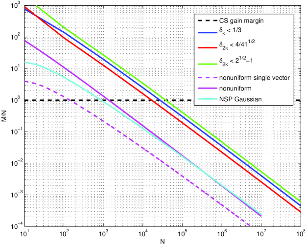
Figure 1: Bounds on compression ratio $M/N$ over system size $N$. Maximal compression to achieve perfect reconstruction with probability $\varepsilon=0.9$ fixed sparsity $k=10$.

From Theorem 1, Theorem 2 and Lemma 1 we devise the following corollary.

Corollary 1.

Let $\boldsymbol{\Phi}$ be a random $M\times N$ matrix with i.i.d. elements distributed according to $\phi_{i,j}\sim\mathcal{C}\mathcal{N}(0,1/M)$. Suppose the measurements are given by $\boldsymbol{z}_{i}=\boldsymbol{\Phi}\boldsymbol{h}_{i}+\boldsymbol{\mu}_{i}$, according to (7), with $\|\boldsymbol{\mu}\|_{2}\leq\xi$. If

$$M\geq 2C_{1}^{2}\delta^{-2}\left(k\ln(eN/k)+\ln(2\varepsilon^{-1})\right),$$

with $\delta\leq\delta_{2k}<1/3$ and $\|\boldsymbol{h}_{i}\|_{2}\leq a_{i}$, then for all $\{\boldsymbol{h}_{i}\}_{i\in\mathcal{N}}$ the solutions $\{\boldsymbol{\hat{h}}_{i}\}_{i\in\mathcal{N}}$ to (19) obey

$$\textnormal{Pr}\left\{\exists i\in\mathcal{N}:\Delta_{i}>2Pq(\boldsymbol{h}_{i},\xi)(2a_{i}+q(\boldsymbol{h}_{i},\xi))\right\}\leq\varepsilon,$$

with $q(\boldsymbol{h}_{i},\xi)=C_{2}(\delta_{k})\frac{\sigma_{k}(\boldsymbol{h}_{i})_{1}}{\sqrt{k}}+2C_{3}(\delta_{k})\xi$ and $C_{2}(\delta),C_{3}(\delta)>0$ as in Theorem 2.

The proof is given in Section VII-B. We point out that, if the number of measurements are in the order of $\mathcal{O}(k\ln(eN/k)$ and, for all $i\in\mathcal{N}$, the channels $\boldsymbol{h}_{i}$ are $k$-sparse (i.e. $\sigma_{k}(\boldsymbol{h}_{i})_{1}=0$), then the rate estimation error $\Delta_{i}$ remains bounded. Moreover, in the noiseless case ($\xi=0$) perfect recovery can be achieved. However, for both cases the system size $N$ must be sufficiently large as said before and illustrated in Figure 1.

IV-D Linear Rate Estimation

In this subsection we derive bounds on the rate gap $\Delta_{i}$ for linear channel gain estimation functions. First, we prove a general theorem that is valid for any linear estimation function defined in Definition 5 and any ensemble of measurement matrices that satisfies the concentration of measure inequality (16). We have the following general result, which is the main result in this chapter.

Theorem 3.

Let channel state information be given by any linear estimation function $\beta(\boldsymbol{z}_{i},j)=|\langle\boldsymbol{\Psi}\boldsymbol{z}_{i},\boldsymbol{e}_{j}\rangle|^{2}$, with $\boldsymbol{\Psi}=\boldsymbol{\Phi}^{H}\boldsymbol{A}$ where $\boldsymbol{A}$ is a positive semi-definite matrix. If $\boldsymbol{\Phi}$ fulfills the concentration inequality (16) and the number of active transmissions is bounded by $1\leq|\mathcal{S}|\leq n$, then for any fixed channels $\boldsymbol{H}=(\boldsymbol{h}_{1},\ldots,\boldsymbol{h}_{N})$ and any $u_{0}\geq 0$, $\rho_{0}\geq 0$ and $\varepsilon\geq 0$,

$$\textnormal{Pr}\left\{\exists\mathcal{S}\subset\mathcal{N},|\mathcal{S}|=n,\exists i\in\mathcal{S}:\Delta_{i}(\mathcal{S})>2P\|\boldsymbol{h}_{i}\|_{2}^{2}(4\sqrt{n}(1+u_{0})\varepsilon+\rho_{0})\right\}\\ \leq\exp(\log(4n^{2})+n\log(Ne/n)-\gamma(\varepsilon))+\exp(n\log(Ne/n))\textnormal{Pr}\left\{s_{\max}(\boldsymbol{\Psi}\boldsymbol{\Phi})>u_{0}\right\}\\ +\exp(n\log(Ne/n))\max_{i\in\mathcal{N}}\textnormal{Pr}\left\{\|\boldsymbol{\Psi}\boldsymbol{\bar{\mu}}_{i}\|_{2}(\|\boldsymbol{\Psi}\boldsymbol{\bar{\mu}}_{i}\|_{2}+2\|\boldsymbol{\Psi}\boldsymbol{\Phi}\boldsymbol{\bar{h}}_{i}\|_{2})>\rho_{0}\right\},$$ (21)

The proof is deferred to Section VII-C. Clearly the bound depends on the choice of $\boldsymbol{\Psi}$ and the distribution of $\boldsymbol{\Phi}$. The latter determines the function $\gamma(\varepsilon)$. However the theorem is rather general and enables the evaluation of different linear estimation functions under different assumptions on the channels and under different distributions of the measurement matrix $\boldsymbol{\Phi}$.

To illustrate the strength of Theorem 3 let us assume that the channel vectors are $k$-sparse, $\boldsymbol{h}_{i}\in\Sigma_{k}$ for all $i$, and consider the following estimation function and measurement matrix. Let the elements of $\boldsymbol{\Phi}$ be distributed complex Gaussian and define the linear estimation function as

$$\beta_{l}(\boldsymbol{z}_{i},j)=|\langle\boldsymbol{\Phi}^{+}\boldsymbol{z}_{i},\boldsymbol{e}_{j}\rangle|^{2},$$ (22)

where $\boldsymbol{\Phi}^{+}$ is defined as the pseudo inverse $\boldsymbol{\Phi}^{+}=\boldsymbol{\Phi}^{H}(\boldsymbol{\Phi}\boldsymbol{\Phi}^{H})^{-1},$ for $M<N$. We devise the following corollary.

Corollary 2.

Under the assumptions of Theorem 3. Let $M<N$. Suppose that the elements of $\boldsymbol{\Phi}$ are distributed $\phi_{i,j}\sim\mathcal{C}\mathcal{N}(0,1/M)$. Let $\beta_{l}(\boldsymbol{z}_{i},j)=|\langle\boldsymbol{\Phi}^{+}\boldsymbol{z}_{i},\boldsymbol{e}_{j}\rangle|^{2}$. Assume that $\|\boldsymbol{e}\|_{2}=0$ and for all $i\in\mathcal{N}$ we have $\boldsymbol{h}_{i}\in\Sigma_{k}$ and $\boldsymbol{h}_{i,j}\sim\mathcal{C}\mathcal{N}(0,1)$ for all $j\in\text{supp}(\boldsymbol{h}_{i})$. We have

$$\textnormal{Pr}\left\{\exists i\in\mathcal{N}:\Delta_{i}>16P\sqrt{\frac{\kappa n}{M}}\left(\sqrt{2}\ln\left(\frac{4nN\left(\genfrac{}{}{0.0pt}{}{N}{n}\right)+1}{\varepsilon}\right)+k\sqrt{\ln\left(\frac{4nN\left(\genfrac{}{}{0.0pt}{}{N}{n}\right)+1}{\varepsilon}\right)}\right)\right\}\leq\varepsilon,$$

with $\kappa=2/(1-\log(2))$.

The proof is given in Section VII-D. A few remarks are in place. For fixed transmit powers $P$, a fixed system size $N$, a given error probability $\varepsilon$ and a fixed number of active links $n$, the rate estimation error scales with $\sqrt{1/M}$, which is also in accordance with the estimation results in [15, Theorem 4.1], where essentially the same scaling is achieved. As was expected, the linear decoding function is not able to achieve perfect recovery (for $M<N$). Perfect recovery can only be achieved by the compressed sensing based decoder but comes at the cost of additional complexity. However, the simulations in the next section show that the linear decoder performs reasonably well when applied to a small systems. Moreover, a linear decoder can be used to perform a subset selection and to reduce the problem size for non-linear algorithms.

V Numerical Examples

We consider a cellular system with one base station and $25$ users. Every node has a single antenna. The users are grouped in $G$ user groups $\mathcal{G}_{g}$, $g=1,2,\ldots,G$. Users within the same user group experience the same path loss. The channels from users in $i\in\mathcal{G}_{f}$ to users $j\in\mathcal{G}_{g}$ are given by

$$h_{j,i}=a_{g,f}b_{j,i}\in\mathbb{C},$$ (23)

where $b_{j,i}\sim\mathcal{C}\mathcal{N}(0,1)$ denotes the small scale fading coefficient and $a_{g,f}$ denotes the distance dependent path loss coefficient, with $a_{g,g}=1$ for all $g$. A similar channel model was used in [28] to model large cellular networks with co-located users. Under certain assumptions the channel matrix $\boldsymbol{H}$ is compressible. More precisely, the matrix $\boldsymbol{H}$ can be approximated by a low rank and/or sparse matrix $\boldsymbol{\hat{H}}$, if the user groups $\mathcal{G}_{g}$ are of sufficient size and/or the path loss coefficients $a_{r,g}$ decay sufficiently fast.

We compare two setups: i) $5$ groups of $5$ users each, the path loss coefficients are chosen as $10^{z/10}$, with $z$ uniformly distributed in $[0,1]$. ii) $25$ users all in the same group and path loss coefficient is $a_{i,g}=1$ for all $i,g$, i.e., all channels are i.i.d. complex Gaussian distributed. The rate requirement is set to $\bar{r}=1/10\log(1+P)$. Problem 19 was solved using the Tfocs toolbox [29].

We compare the solution to problem (13) for the non-linear compressed sensing estimation function (19) and the linear estimation function (22). In the simulations $\varepsilon=0$, since the analytic results do not give tight bounds for systems with $N=25$. Nevertheless the results in Figure 2 show that linear estimation performs very close to the much more complex compressed sensing based estimation. Figure 3 shows that if the channel matrix is compressible the compressed sensing estimation function performs better than the linear estimation function. Since the considered systems are rather small it can be expected that the gain of compressed sensing increases for larger systems.

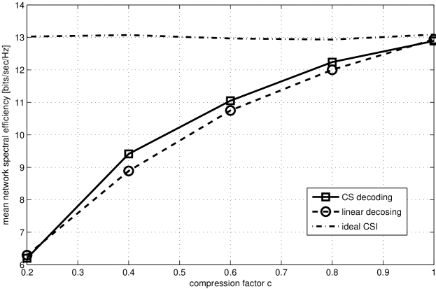
Figure 2: Average sum-rate over compression factor $M/N$; Setup: $25$ users, $1$ base station, perfect feedback channel (no feedback and quantization noise), single group; channel matrix i.i.d. Gauss and not compressible. Comparison of linear and non-linear rate estimation.

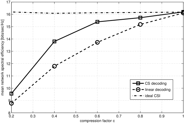
Figure 3: Average sum-rate over compression factor $M/N$; Setup: $25$ users, $1$ base station, perfect feedback channel (no feedback and quantization noise), 5 group of 5 users each; channel matrix compressible, single group; channel matrix i.i.d. Gauss and not compressible. Comparison of linear and non-linear rate estimation.

VI Conclusion

We developed a channel sensing and reconstruction protocol that enables the network controller to estimate the achievable rates based on compressed non-adaptive measurements. The scaling of the estimation error at the network controller has been analyzed for linear and non-linear decoding functions. Scaling results for the non-linear decoding function where shown to follow from well known compressed sensing results. However, for a small to moderate system size $N$ the compressed sensing results do not provide reasonable performance bounds. For linear decoding functions we derived a general result which can be used to analyze the performance of a variety of linear decoding functions and measurement matrices. For a linear decoding function based on the pseudo inverse and Gaussian measurement matrices we investigated the scaling of the rate estimation error with the number of measurements.

The measurement protocol is based on a few simplifications which render the direct application in practical systems rather difficult. For example, the assumption of perfect time and frequency synchronization is hard (if not impossible) to achieve in distributed networks with a huge number of devices. To this end, the analog coding developed in [13] can be used to relax the requirements on the synchronization.

Future work may also include the exploration of different linear and non-linear decoding functions. To this end, Theorem 3 provides a good basis to evaluate different linear decoding functions. For non-linear decoding functions applications of matrix recovery and other compressed sensing related approaches are a promising research direction. Extensions to other network architectures are another prospective direction. Coordinated transmission techniques where groups of devices (or antennas) are jointly transmitting with beamforming vectors $\boldsymbol{w}$ given by some finite codebook can be analyzed with the proposed framework by estimating $|\langle\boldsymbol{h}_{i},\boldsymbol{w}\rangle|$.

VII Proofs

VII-A Proof of Lemma 1

Proof:

For each $i$ the corresponding rate gap $\Delta_{i}$ can rewritten using the abbreviations $L(s):=\log(1+s)$, $q_{j}:=p_{j}|h_{i,j}|^{2}$ and $\hat{q}_{j}:=p_{j}|\hat{h}_{i,j}|^{2}$:

$$\begin{split}\Delta_{i}&=\left|L\left(\frac{q_{j}}{1+\sum_{l\in\mathcal{S}\setminus\{i\}}q_{l}}\right)-L\left(\frac{\hat{q}_{j}}{1+\sum_{l\in\mathcal{S}\setminus\{i\}}\hat{q}_{l}}\right)\right|\\ &=\left|\log\left(\frac{1+\sum_{l\in\mathcal{S}}q_{l}}{1+\sum_{l\in\mathcal{S}}\hat{q}_{l}}\right)+\log\left(\frac{1+\sum_{l\in\mathcal{S}\setminus\{i\}}\hat{q}_{l}}{1+\sum_{l\in\mathcal{S}\setminus\{i\}}q_{l}}\right)\right|\\ &=\left|L\left(\frac{\sum_{l\in\mathcal{S}}q_{l}-\hat{q}_{l}}{1+\sum_{l\in\mathcal{S}}\hat{q}_{l}}\right)+L\left(\frac{\sum_{l\in\mathcal{S}\setminus\{i\}}\hat{q}_{l}-q_{l}}{1+\sum_{l\in\mathcal{S}\setminus\{i\}}q_{l}}\right)\right|\\ &\leq\Biggl{|}L\left(\frac{\sum_{l\in\mathcal{S}}q_{l}-\hat{q}_{l}}{1+\sum_{l\in\mathcal{S}}\hat{q}_{l}}\right)\Biggr{|}+\Biggl{|}L\left(\frac{\sum_{l\in\mathcal{S}\setminus\{i\}}\hat{q}_{l}-q_{l}}{1+\sum_{l\in\mathcal{S}\setminus\{i\}}q_{l}}\right)\Biggr{|}\\ &\leq 2L\left(\sum_{l\in\mathcal{S}}|q_{l}-\hat{q}_{l}|\right),\end{split}$$ (24)

where the first inequality follows from the triangle inequality and the second inequality follows from Jensen’s inequality and the fact that the denominators are positive. Since, $L(x)\leq x$ for $x\geq 0$ and by assumption $p_{j}\leq P$, for all $j$, we obtain the first claim

$$\Delta_{i}\leq 2P\sum_{l\in\mathcal{S}}||h_{i,l}|^{2}-|\hat{h}_{i,l}|^{2}|.$$

∎

VII-B Proof of Corollary 1

Proof:

Using Lemma 1, the Cauchy-Schwarz inequality and the reverse triangle inequality we get

$$\Delta_{i} \leq 2P\sum_{j\in\mathcal{S}}|x_{i,j}-\hat{x}_{i,j}|$$ (25)

$$\leq 2P\sum_{j\in\mathcal{N}}|(|h_{i,j}|-|\hat{h}_{i,j}|)(|h_{i,j}|+|\hat{h}_{i,j}|)|$$ (26)

$$\leq 2P\left\|\boldsymbol{h}_{i}-\boldsymbol{\hat{h}}_{i}\right\|_{2}\left\||\boldsymbol{h}_{i}|+|\boldsymbol{\hat{h}}_{i}|\right\|_{2}$$ (27)

$$\leq 2P\left\|\boldsymbol{h}_{i}-\boldsymbol{\hat{h}}_{i}|\right\|_{2}\left(2\|\boldsymbol{h}_{i}\|_{2}+\left\|\boldsymbol{h}_{i}-\boldsymbol{\hat{h}_{i}}\right\|_{2}\right).$$ (28)

By assumption $M\geq 2C_{1}^{2}\delta^{-2}\left(k\ln(eN/k)+\ln(2\varepsilon^{-1})\right)$, with $\delta<1/3$, such that $\boldsymbol{\Phi}$ satisfies the RIP with probability at least $1-\varepsilon$. Hence, we can use Theorem 2 and plug (20) in (28). Finally, defining $q(\boldsymbol{h}_{i},\xi)=C_{2}(\delta_{k})\frac{\sigma_{k}(\boldsymbol{h}_{i})_{1}}{\sqrt{k}}+2C_{3}(\delta_{k})\xi$ the claim follows. ∎

VII-C Proof of Theorem 3

The prove of Theorem 3 is developed in several steps.

Lemma 2.

Let $X$ and $Y$ be two non-negative real random variables. If $f:\mathbb{R}\times\mathbb{R}\rightarrow\mathbb{R}$ is monotonically increasing in the second input and $y_{0}>0$ is a positive constant, then

$$\textnormal{Pr}\left\{f(X,Y)>\varepsilon\right\}\leq\min_{y_{0}\geq 0}\textnormal{Pr}\left\{f(X,y_{0})>\varepsilon\right\}+\textnormal{Pr}\left\{Y>y_{0}\right\}.$$

Proof:

First assume that the random variable $Y$ is bounded by $Y>y_{0}$. In this case the claim is trivially true, since $\textnormal{Pr}\left\{Y>y_{0}\right\}=1$. Therefore, assume that $\textnormal{Pr}\left\{Y\leq y_{0}\right\}>0$. We will abbreviate $Z=f(X,Y)$ and $Z_{0}=f(X,y_{0})$. For any arbitrary but fixed $y_{0}\geq 0$ we have,

$$\begin{split}&\textnormal{Pr}\left\{Z>\varepsilon\right\}=1-\textnormal{Pr}\left\{Z\leq\varepsilon|Y\leq y_{0}\right\}-\textnormal{Pr}\left\{Z\leq\varepsilon|Y>y_{0}\right\}\\ &\leq 1-\textnormal{Pr}\left\{Z\leq\varepsilon|Y\leq y_{0}\right\}\leq 1-\textnormal{Pr}\left\{Z_{0}\leq\varepsilon|Y\leq y_{0}\right\}\\ &=1-\frac{\textnormal{Pr}\left\{\{Z_{0}\leq\varepsilon\}\cap\{Y\leq y_{0}\}\right\}}{\textnormal{Pr}\left\{Y\leq y_{0}\right\}}\\ &=1-\frac{1-\textnormal{Pr}\left\{\{Z_{0}>\varepsilon\}\cup\{Y>y_{0}\}\right\}}{\textnormal{Pr}\left\{Y\leq y_{0}\right\}}\\ &\leq 1-\frac{1-\textnormal{Pr}\left\{Z_{9}>\varepsilon\right\}-\textnormal{Pr}\left\{Y>y_{0}\right\}}{\textnormal{Pr}\left\{Y\leq y_{0}\right\}}\\ &\leq\textnormal{Pr}\left\{Z_{0}>\varepsilon\right\}+\textnormal{Pr}\left\{Y>y_{0}\right\},\end{split}$$ (29)

where we first used De Morgan’s law and then the union bound. ∎

Lemma 3.

Let $\mathcal{V}=\{\boldsymbol{v}_{1},\ldots,\boldsymbol{v}_{n}\}\subset\mathbb{S}^{N-1}$ be an arbitrary but fixed set of mutually orthogonal vectors ($n\leq N$), $\boldsymbol{\Psi}=\boldsymbol{\Phi}^{H}\boldsymbol{A}\in\mathbb{C}^{N\times M}$ and $\boldsymbol{A}\in\mathbb{C}^{M\times M}$ be a positive semi-definite matrix. If $\boldsymbol{w}=\boldsymbol{\Phi}\boldsymbol{u}+\boldsymbol{e}$ and $\boldsymbol{\Phi}$ is a $M\times N$ random matrix that is isotropically distributed and satisfies the concentration inequality (16), then for any fixed $\boldsymbol{u}\in\mathbb{S}^{N-1}$ and any fixed $\boldsymbol{e}\in\mathbb{C}^{M}$

$$\begin{split}\@ADDCLASS{ltx_eqn_lefteqn}$\displaystyle\textnormal{Pr}\left\{\left|\sum_{i=1}^{n}|\langle\boldsymbol{u},\boldsymbol{v}_{i}\rangle|^{2}-|\langle\boldsymbol{\Psi}\boldsymbol{w},\boldsymbol{v}_{i}\rangle|^{2}\right|>4\sqrt{n}(1+u_{0})\varepsilon+\rho_{0}\right\}$\mbox{}\hfil\\ &\leq 4n\exp(-\gamma\left(\varepsilon\right))+\textnormal{Pr}\left\{s_{\max}(\boldsymbol{\Psi}\boldsymbol{\Phi})>u_{0}\right\}\\ &\quad+\textnormal{Pr}\left\{\|\boldsymbol{\Psi}\boldsymbol{e}\|_{2}(\|\boldsymbol{\Psi}\boldsymbol{e}\|_{2}+2\|\boldsymbol{\Psi}\boldsymbol{\Phi}\boldsymbol{u}\|_{2})>\rho_{0}\right\}\end{split}$$ (30)

holds, where $\gamma(\varepsilon)$ depends on the distribution of $\boldsymbol{\Phi}$ and $\rho_{0},u_{0}\geq 0$ are positive constants.

Proof:

Consider the vectors $\boldsymbol{a},\boldsymbol{b},\boldsymbol{c}\in\mathbb{C}^{n}$ with elements $a_{i}=\langle\boldsymbol{u},\boldsymbol{v}_{i}\rangle$, $b_{i}=\langle\boldsymbol{\Psi}\boldsymbol{\Phi}\boldsymbol{u},\boldsymbol{v}_{i}\rangle$ and $c_{i}=\langle\boldsymbol{\Psi}\boldsymbol{e},\boldsymbol{v}_{i}\rangle$. Obviously $\lVert\boldsymbol{a}\rVert_{2}\leq 1$, $\lVert\boldsymbol{b}\rVert_{2}\leq\lVert\boldsymbol{\Psi}\boldsymbol{\Phi}\boldsymbol{u}\rVert_{2}$ and $\lVert\boldsymbol{c}\rVert_{2}\leq\lVert\boldsymbol{\Psi}\boldsymbol{e}\rVert_{2}$.

$$\begin{split}D:=&\sum_{i=1}^{n}\left||a_{i}|^{2}-|b_{i}+c_{i}|^{2}\right|=\sum_{i=1}^{n}\left||a_{i}|^{2}-|b_{i}|^{2}-|c_{i}|^{2}-2\Re\left(b_{i}\bar{c}_{i}\right)\right|\\ &\leq\sum_{i=1}^{n}\left||a_{i}|^{2}-|b_{i}|^{2}\right|+|c_{i}|^{2}+2|b_{i}\bar{c}_{i}|\\ &\leq\sum_{i=1}^{n}\left||a_{i}|^{2}-|b_{i}|^{2}\right|+\lVert\boldsymbol{c}\rVert(1+2\lVert\boldsymbol{b}\rVert)\\ &=\sum_{i=1}^{n}\left|(|a_{i}|-|b_{i}|)(|a_{i}|+|b_{i}|)\right|+\lVert\boldsymbol{c}\rVert_{2}(1+2\lVert\boldsymbol{b}\rVert_{2})\\ &\leq\lVert|\boldsymbol{a}|-|\boldsymbol{b}|\rVert_{p}\cdot\lVert|\boldsymbol{a}|+|\boldsymbol{b}|\rVert_{q}+\lVert\boldsymbol{c}\rVert_{2}(1+2\lVert\boldsymbol{b}\rVert_{2})\\ &\leq\lVert\boldsymbol{a}-\boldsymbol{b}\rVert_{p}\cdot(\lVert\boldsymbol{a}\rVert_{q}+\lVert\boldsymbol{b}\rVert_{q})+\lVert\boldsymbol{c}\rVert_{2}(1+2\lVert\boldsymbol{b}\rVert_{2})\end{split}$$ (31)

Recall, that $\boldsymbol{b}$ and $\boldsymbol{c}$ are random vectors. We apply now Lemma 2 twice. First, for the non–negative random variables $X=\lVert\boldsymbol{a}-\boldsymbol{b}\rVert_{p}\cdot(\lVert\boldsymbol{a}\rVert_{q}+\lVert\boldsymbol{b}\rVert_{q})$ and $Y=\lVert\boldsymbol{c}\rVert_{2}(1+2\lVert\boldsymbol{b}\rVert_{2})$, for any $0\leq\rho_{0}$, we have,

$$\begin{split}\textnormal{Pr}\left\{D>\varepsilon^{\prime}\right\}\leq&\underbrace{\textnormal{Pr}\left\{\lVert\boldsymbol{a}-\boldsymbol{b}\rVert_{p}\cdot(\lVert\boldsymbol{a}\rVert_{q}+\lVert\boldsymbol{b}\rVert_{q})+\rho_{0}>\varepsilon^{\prime}\right\}}_{(i)}+\textnormal{Pr}\left\{\lVert\boldsymbol{c}\rVert(1+2\lVert\boldsymbol{b}\rVert)>\rho_{0}\right\}.\end{split}$$ (32)

Second, for $X=\lVert\boldsymbol{a}-\boldsymbol{b}\rVert_{p}$ and $Y=\lVert\boldsymbol{a}\rVert_{q}+\lVert\boldsymbol{b}\rVert_{q}$, for any $y_{0}>0$, we have,

$$\begin{split}\text{(i)}&=\textnormal{Pr}\left\{\lVert\boldsymbol{a}-\boldsymbol{b}\rVert_{p}\cdot(\lVert\boldsymbol{a}\rVert_{q}+\lVert\boldsymbol{b}\rVert_{q})>\varepsilon^{\prime}-\rho_{0}\right\}\\ &\leq\textnormal{Pr}\left\{\lVert\boldsymbol{a}-\boldsymbol{b}\rVert_{p}>\frac{\varepsilon^{\prime}-\rho_{0}}{y_{0}}\right\}+\textnormal{Pr}\left\{\lVert\boldsymbol{a}\rVert_{q}+\lVert\boldsymbol{b}\rVert_{q}\geq y_{0}\right\}\end{split}$$ (33)

By assumption $\boldsymbol{\Psi}=\boldsymbol{\Phi}^{H}\boldsymbol{A}=\boldsymbol{\Phi}^{H}\boldsymbol{A}^{1/2}\boldsymbol{A}^{1/2}$, where $\boldsymbol{A}^{1/2}$ is the principal square root of $\boldsymbol{A}$. From the definition of $\boldsymbol{a}$ and $\boldsymbol{b}$ it follows that

$$\lVert\boldsymbol{a}-\boldsymbol{b}\rVert_{p}=\lVert\{|\langle\boldsymbol{u},\boldsymbol{v}_{i}\rangle-\langle\boldsymbol{B}\boldsymbol{u},\boldsymbol{B}\boldsymbol{v}_{i}\rangle|\}_{i=1}^{n}\rVert_{p}\leq\lVert\boldsymbol{m}\rVert_{p},$$ (34)

where the $n$ components $m_{i}$ of the vector $\boldsymbol{m}$ follow from the polarization identity as,

$$\begin{split}|a_{i}-b_{i}|&=\frac{1}{4}\Bigl{|}\sum_{\xi\in\{\pm 1,\pm i\}}\xi(\|\boldsymbol{u}+\xi\boldsymbol{v}_{i}\|_{2}^{2}-\|\boldsymbol{B}(\boldsymbol{u}+\xi\boldsymbol{v}_{i})\|_{2}^{2})\Bigr{|}\\ &\leq\frac{1}{4}\sum_{\xi\in\{\pm 1,\pm i\}}\Bigl{|}\|\boldsymbol{u}+\xi\boldsymbol{v}_{i}\|_{2}^{2}-\|\boldsymbol{B}(\boldsymbol{u}+\xi\boldsymbol{v}_{i})\|_{2}^{2}\Bigr{|}\\ &\leq\max_{\xi\in\{\pm 1,\pm i\}}\Bigl{|}\|\boldsymbol{u}+\xi\boldsymbol{v}_{i}\|_{2}^{2}-\|\boldsymbol{B}(\boldsymbol{u}+\xi\boldsymbol{v}_{i})\|_{2}^{2}\Bigr{|}=:m_{i}.\end{split}$$ (35)

Thus, we have

$$\begin{split}\text{(i)}&\leq\textnormal{Pr}\left\{\lVert\boldsymbol{m}\rVert_{p}>\frac{\varepsilon^{\prime}-\rho_{0}}{y_{0}}\right\}+\textnormal{Pr}\left\{\lVert\boldsymbol{a}\rVert_{q}+\lVert\boldsymbol{b}\rVert_{q}\geq y_{0}\right\}.\end{split}$$ (36)

Next, we use $p=\infty$, $q=1$, $\lVert\boldsymbol{a}\rVert_{1}\leq\sqrt{n}$ and $\lVert\boldsymbol{b}\rVert_{1}\leq\sqrt{n}\lVert\boldsymbol{b}\rVert_{2}$. By assumption $\boldsymbol{\Phi}$ is isotropically distributed, i.e., each component of $\boldsymbol{m}$ has the same distribution. Thus, $\lVert\boldsymbol{m}\rVert_{\infty}$ is the maximum over $4n$ identically distributed random variables. Define $u_{0}=y_{0}/\sqrt{n}-1$. Using the union bound and the concentration inequality (16) we have,

$$\begin{split}\text{(i)}&\leq 4n\textnormal{Pr}\left\{|m_{1}|>\frac{\varepsilon^{\prime}-\rho_{0}}{y_{0}}\right\}+\textnormal{Pr}\left\{\lVert\boldsymbol{b}\rVert_{2}\geq\frac{y_{0}}{\sqrt{n}}-1\right\}\\ &=4n\textnormal{Pr}\left\{|m_{1}|>\frac{\varepsilon^{\prime}-\rho_{0}}{\sqrt{n}(u_{0}+1)}\right\}+\textnormal{Pr}\left\{\lVert\boldsymbol{b}\rVert_{2}\geq u_{0}\right\}\\ &\leq 4n\exp(-\gamma(\frac{\varepsilon^{\prime}-\rho_{0}}{\|\boldsymbol{u}+\boldsymbol{v}_{1}\|_{2}^{2}\sqrt{n}(1+u_{0})}))+\textnormal{Pr}\left\{\lVert\boldsymbol{b}\rVert_{2}\geq u_{0}\right\}\\ &\leq 4n\exp(-\gamma(\frac{\varepsilon^{\prime}-\rho_{0}}{4\sqrt{n}(1+u_{0})}))+\textnormal{Pr}\left\{\lVert\boldsymbol{b}\rVert_{2}\geq u_{0}\right\}\\ &\leq 4n\exp(-\gamma(\varepsilon))+\textnormal{Pr}\left\{\lVert\boldsymbol{b}\rVert_{2}\geq u_{0}\right\}\\ \end{split}$$ (37)

The last steps follow from $\|\boldsymbol{u}+\boldsymbol{v}_{1}\|_{2}^{2}\leq 4$ and with $\varepsilon^{\prime}=\varepsilon 4\sqrt{n}(1+u_{0})+\rho_{0}$. Since $\textnormal{Pr}\left\{\|\boldsymbol{\Psi}\boldsymbol{\Phi}\boldsymbol{u}\|_{2}>u_{0}\right\}\leq\textnormal{Pr}\left\{s_{\max}(\boldsymbol{\Psi}\boldsymbol{\Phi})>u_{0}\right\}$ the claim follows from the last equation and (32). ∎

Now we are ready to prove Theorem 3.

Proof:

Let $\mathcal{S}\subseteq\mathcal{N}$ be arbitrary but fixed. By the assumptions the rate gap bound in Lemma 1 can be rewritten as

$$\Delta_{i}(\mathcal{S})\leq 2P\|\boldsymbol{h}_{i}\|_{2}^{2}\sum_{l\in\mathcal{S}}\left||\langle\boldsymbol{\bar{h}}_{i},\boldsymbol{e}_{l}\rangle|^{2}-|\langle\boldsymbol{\Psi}(\boldsymbol{\Phi}\boldsymbol{\bar{h}}_{i}+\boldsymbol{\bar{\mu}}_{i}),\boldsymbol{e}_{l}\rangle|^{2}\right|,$$

where we defined $\boldsymbol{\bar{h}}_{i}=\boldsymbol{h}_{i}/\|\boldsymbol{h}_{i}\|_{2}$ and $\boldsymbol{\bar{\mu}}_{i}=\boldsymbol{\mu}_{i}/\|\boldsymbol{h}_{i}\|_{2}$. If we fix $|\mathcal{S}|=n$, Lemma 3 yields

$$\textnormal{Pr}\left\{\Delta_{i}(\mathcal{S})>2P\|\boldsymbol{h}_{i}\|_{2}^{2}(4\sqrt{n}(1+u_{0})\varepsilon+\rho_{0})\right\}\leq 4n\exp(-\gamma(\varepsilon))+\\ \textnormal{Pr}\left\{s_{\max}(\boldsymbol{\Psi}\boldsymbol{\Phi})>u_{0}\right\}+\textnormal{Pr}\left\{\|\boldsymbol{\Psi}\boldsymbol{\bar{\mu}}_{i}\|_{2}\left(\|\boldsymbol{\Psi}\boldsymbol{\bar{\mu}}_{i}\|_{2}+2\|\boldsymbol{\Psi}\boldsymbol{\Phi}\boldsymbol{\bar{h}}_{i}\|_{2}\right)>\rho_{0}\right\},$$ (38)

for an arbitrary $i\in\mathcal{S}$. Taking the union bound over all $i\in\mathcal{S}$ yields,

$$\textnormal{Pr}\left\{\exists i\in\mathcal{S}:\Delta_{i}(\mathcal{S})>2P\|\boldsymbol{h}_{i}\|_{2}^{2}(4\sqrt{n}(1+u_{0})\varepsilon+\rho_{0})\right\}\leq 4n^{2}\exp(-\gamma(\varepsilon))+\\ n\textnormal{Pr}\left\{s_{\max}(\boldsymbol{\Psi}\boldsymbol{\Phi})>u_{0}\right\}+\sum_{i\in\mathcal{S}}\textnormal{Pr}\left\{\|\boldsymbol{\Psi}\boldsymbol{\bar{\mu}}_{i}\|_{2}(\|\boldsymbol{\Psi}\boldsymbol{\bar{\mu}}_{i}\|_{2}+2\|\boldsymbol{\Psi}\boldsymbol{\Phi}\boldsymbol{\bar{h}}_{i}\|_{2})>\rho_{0}\right\},$$ (39)

Finally, applying the union bound over all $\binom{N}{n}$ scheduling decisions $\mathcal{S}\subseteq\mathcal{N}$, with $|\mathcal{S}|=n$,

$$\textnormal{Pr}\left\{\exists\mathcal{S}\subset\mathcal{N},|\mathcal{S}|=n,\exists i\in\mathcal{S}:\Delta_{i}(\mathcal{S})>2P\|\boldsymbol{h}_{i}\|_{2}^{2}(4\sqrt{n}(1+u_{0})\varepsilon+\rho_{0})\right\}\\ \leq\exp(\log(4n^{2})+n\log(Ne/n)-\gamma(\varepsilon))+\exp(n\log(Ne/n))\textnormal{Pr}\left\{s_{\max}(\boldsymbol{\Psi}\boldsymbol{\Phi})>u_{0}\right\}\\ +\exp(n\log(Ne/n))\max_{i\in\mathcal{N}}\textnormal{Pr}\left\{\|\boldsymbol{\Psi}\boldsymbol{\bar{\mu}}_{i}\|_{2}(\|\boldsymbol{\Psi}\boldsymbol{\bar{\mu}}_{i}\|_{2}+2\|\boldsymbol{\Psi}\boldsymbol{\Phi}\boldsymbol{\bar{h}}_{i}\|_{2})>\rho_{0}\right\},$$ (40)

where we used $\binom{N}{n}\leq(Ne/n)^{n}$.

∎

VII-D Proof of Corollary 2

The following result will be useful in the proof. Let $\boldsymbol{a}$ be a random vector with elements $a_{i}\sim\mathcal{C}\mathcal{N}(0,1)$. Then, for all $t>0$,

$$\textnormal{Pr}\left\{\|\boldsymbol{a}\|_{2}^{2}-\mathbb{E}\left[{\|\boldsymbol{a}\|_{2}^{2}}\right]>t\right\}\leq\exp(-t^{2}/2).$$ (41)

In fact, this is a special case of the concentration of measure theorem for Lipschitz functions, see [24, Theorem 8.40].

Proof:

For an arbitrary but fixed $\boldsymbol{h}_{i}$. Setting $e_{0}=0$, we have

$$\textnormal{Pr}\left\{\|\boldsymbol{\Psi}\boldsymbol{e}\|_{2}(\|\boldsymbol{\Psi}\boldsymbol{e}\|_{2}+2\|\boldsymbol{\Psi}\boldsymbol{\Phi}\boldsymbol{u}\|_{2})>e_{0}\right\}=0.$$

Since $\boldsymbol{\Phi}^{+}\boldsymbol{\Phi}$ is a projector (i.e. Hermitian and idempotent) $s_{\max}(\boldsymbol{\Phi}^{+}\boldsymbol{\Phi})=1$, and therefore we can set $u_{0}=1$ and obtain $\textnormal{Pr}\left\{s_{\max}(\boldsymbol{\Psi}\boldsymbol{\Phi})>1\right\}=0.$ Using (18) we get from Theorem 3

$$\textnormal{Pr}\left\{\exists\mathcal{S}\subset\mathcal{N},|\mathcal{S}|\leq n\leq N/2:\Delta_{i}>16P\|\boldsymbol{h}_{i}\|^{2}_{2}\sqrt{n}\varepsilon^{\prime})\right\}\leq 4nN\left(\genfrac{}{}{0.0pt}{}{N}{n}\right)\exp\left(-M\varepsilon^{\prime 2}/\kappa\right),$$

with $\kappa=\frac{2}{1-\ln(2)}$. Since $\boldsymbol{h}_{i}$ is also random we can use Lemma 2 and get

$$\textnormal{Pr}\left\{\exists i\in\mathcal{N}:\Delta_{i}>16Ph_{0}\sqrt{n}\varepsilon^{\prime})\right\}\leq 4nN\left(\genfrac{}{}{0.0pt}{}{N}{n}\right)\exp\left(-M\varepsilon^{\prime 2}/\kappa\right)+\textnormal{Pr}\left\{\|\boldsymbol{h}_{i}\|^{2}_{2}>h_{0}\right\}.$$

By assumption we have $\mathbb{E}\left[{\|\boldsymbol{h}_{i}\|^{2}_{2}}\right]=k$. Thus, (41) gives,

$$\textnormal{Pr}\left\{\|\boldsymbol{h}_{i}\|^{2}_{2}>h_{0}\right\}=\textnormal{Pr}\left\{\|\boldsymbol{h}_{i}\|^{2}_{2}>t+k\right\}\leq\exp(-t^{2}/2).$$

Hence, if we set $h_{0}=t+k$ and $t=\sqrt{2M\varepsilon^{\prime 2}/\kappa}$,

$$\textnormal{Pr}\left\{\exists i\in\mathcal{N}:\Delta_{i}>16P\sqrt{n}(\sqrt{2M\varepsilon^{\prime 2}/\kappa}+k)\varepsilon^{\prime})\right\}\leq\left(4nN\left(\genfrac{}{}{0.0pt}{}{N}{n}\right)+1\right)\exp\left(-M\varepsilon^{\prime 2}/\kappa\right).$$

Finally, setting $\varepsilon=(4nN+1)\exp\left(-M\varepsilon^{\prime 2}/\kappa\right)$ the claim follows. ∎

References

- [1] P. Popovski, V. Braun, H. P.Mayer, P. Fertl, and et al., “Scenarios, requirements and KPIs for 5G mobile and wireless systems.” The METIS project: Mobile and wireless communications Enablers for the Twenty-twenty Information Society, Tech. Rep. ICT-317669-METIS/D1.1, 2013, https://www.metis2020.com.
- [2] K. Doppler, M. Rinne, C. Wijting, C. B. Riberio, and K. Hugl, “D2D communications underlaying an LTE cellular network,” IEEE Communications Magazine, vol. 7, no. 12, pp. 42–49, December 2009.
- [3] M. S. Corson, “Towards proximity-aware internetworking,” IEEE Wireless Commun. Mag., vol. 17, no. 6, pp. 26–33, Dec. 2010.
- [4] G. Fodor, E. Dahlman, G. Mildh, S. Parkvall, N. Reider, G. Miklos, and Z. Turanyi, “Design aspects of network assisted device-to-device communications,” IEEE Communications Magazine, vol. 50, no. 3, pp. 170–177, 2012.
- [5] N. Lee, X. Lin, J. Andrews, and R. Heath, “Power control for D2D underlaid cellular networks: Modeling, algorithms and analysis,” http://arxiv.org/abs/1305.6161, 2013.
- [6] M. Belleschi, G. Fodor, and A. Abrardo, “Performance Analysis of a Distributed Resource Allocation Sceheme for D2D Communications,” in IEEE Workshop on Machine-to-Machine Communications. IEEE, 2011.
- [7] S. Shakkottai, T. S. Rappaport, and P. Karlson, “Cross-layer design for wireless networks,” IEEE Communications Magazine, 2003.
- [8] B. Kaufman, J. Lilleberg, and B. Aazhang, “Spectrum sharing scheme between cellular users and ad-hoc device-to-device users,” CoRR, vol. abs/1301.6980, 2013.
- [9] 3GPP, “3rd Generation Partnership Project; Technical Specification Group Services and System Aspects; Feasibility study for Proximity Services (ProSe) (Release 12),” 3GPP TR 22.803, Tech. Rep., 2013.
- [10] ——, “3rd Generation Partnership Project; Technical Specification Group Services and System Aspects; Study on architecture enhancements to support Proximity-based Services (ProSe),” 3GPP TR 23.703, Tech. Rep., 2014.
- [11] J. Schreck, P. Jung, and S. Stanczak, “On channel state feedback for two-hop networks based on low rank matrix recovery,” in IEEE International Conference on Communications (ICC), 2013, pp. 3024–3028.
- [12] M. Belleschi, G. Fodor, D. D. Penda, M. Johansson, A. Pradini, and A. Abrardo, “Benchmarking practical RRM algorithms for D2D communications in LTE advanced,” Arxiv preprint arxiv:1306.5305v1, 2013. [Online]. Available: http://arxiv.org/abs/1306.5305
- [13] M. Goldenbaum and S. Stanczak, “Robust analog function computation via wireless sensor multiple-access channels,” IEEE Trans. Commun., 2013, (to appear, preprint available at http://arxiv.org/abs/1210.2967).
- [14] E. J. Candes, J. K. Romberg, and T. Tao, “Stable signal recovery from incomplete and inaccurate measurements,” Communications on pure and applied mathematics, vol. 59, no. 8, pp. 1207–1223, 2006.
- [15] M. A. Davenport, M. B. Wakin, and R. G. Baraniuk, “Detection and estimation with compressive measurements,” Dept. of ECE, Rice University, Tech. Rep, 2006.
- [16] R. Baraniuk, M. Davenport, R. A. DeVore, and M. Wakin, “A Simple Proof of the Restricted Isometry Property for Random Matrices,” Constructive Approximation, vol. 28, no. 3, pp. 253–263, Jan. 2008.
- [17] P. Jung and P. Walk, “Sparse Model Uncertainties in Compressed Sensing with Application to Convolutions and Sporadic Communication,” in to appear in Compressed Sensing and its Applications, J. V. Holger Boche, Robert Calderbank, Gitta Kutyniok, Ed. Springer, 2015, pp. 1–29. [Online]. Available: http://arxiv.org/abs/1404.0218
- [18] M. Ledoux, The Concentration of Measure Phenomenon, ser. Mathematical Surveys and Monographs. Providence, Rhode Island: American Mathematical Society, Feb. 2005, vol. 89.
- [19] T. Tao, Topics in random matrix theory. American Mathematical Society, 2012.
- [20] R. Vershynin, “Introduction to the non-asymptotic analysis of random matrices,” arXiv preprint arXiv:1011.3027, pp. 210–268, 2010. [Online]. Available: http://arxiv.org/abs/1011.3027
- [21] M. Davenport, “Concentration of measure for sub-Gaussian random variables,” OpenStax CNX, pp. 1–5, 2011.
- [22] F. Krahmer and R. Ward, “New and improved Johnson-Lindenstrauss embeddings via the Restricted Isometry Property,” SIAM Journal on Mathematical Analysis, vol. 43, no. 3, pp. 1269–1281, 2011.
- [23] D. G. Luenberger, Optimization by vector space methods. New York, NY, USA: John Wiley & Sons, Inc., 1968.
- [24] S. Foucart and H. Rauhut, A Mathematical Introduction to Compressive Sensing, ser. Applied and Numerical Harmonic Analysis. New York, NY: Springer New York, 2013.
- [25] Y. Eldar and G. Kutyniok, Compressed sensing: theory and applications. Cambridge University Press, 2012.
- [26] T. T. Cai and A. Zhang, “Sharp RIP bound for sparse signal and low-rank matrix recovery,” Applied and Computational Harmonic Analysis, vol. 35, no. 1, pp. 74–93, Jul. 2013.
- [27] T. Cai and A. Zhang, “Sparse representation of a polytope and recovery of sparse signals and low-rank matrices,” Information Theory, IEEE Transactions on, vol. 60, no. 1, pp. 122–132, Jan 2014.
- [28] H. Huh, A. M. Tulino, and G. Caire, “Network MIMO with linear zero-forcing beamforming: large system analysis, impact of channel estimation and reduced-complexity scheduling,” IEEE Transactions on Information Theory, no. 5, pp. 2911–2934, 2010.
- [29] S. Becker, E. Candes, and M. Grant, “Tfocs: Flexible first-order methods for rank minimization,” in Low-rank Matrix Optimization Symposium, SIAM Conf. on Optimization, 2011.