Variable Viscosity and Density Biofilm Simulations using an Immersed Boundary Method, Part II: Experimental Validation and the Heterogeneous Rheology-IBM

Abstract

The goal of this work is to develop a numerical simulation that accurately captures the biomechanical response of bacterial biofilms and their associated extracellular matrix (ECM). In this, the second of a two-part effort, the primary focus is on formally presenting the heterogeneous rheology Immersed Boundary Method (hrIBM) and validating our model against experimental results. With this extension of the Immersed Bounadry Method (IBM), we use the techniques originally developed in Part I, (Hammond et al. [15]) to treat the biofilm as a viscoelastic fluid possessing variable rheological properties anchored to a set of moving locations (i.e., the bacteria locations). We validate our modeling approach from Part I by comparing dynamic moduli and compliance moduli computed from our model to data from mechanical characterization experiments on Staphylococcus epidermidis biofilms. The experimental setup is described in Pavlovsky et al. (2013) [22] in which biofilms are grown and tested in a parallel plate rheometer. Matlab code used to produce results in this paper will be available at https://github.com/MathBioCU/BiofilmSim.

1 Introduction

The goal of this work is to develop a numerical simulation method that accurately captures the biomechanical response of bacterial biofilms and their associated extracellular matrix (ECM). In this second paper, we show that the model and simulation method developed in part I [15], can be used to predict material properties of a biofilm and that the simulated results mimic experimentally measured results. The underlying mathematical technique is an adaptation of the Immersed Boundary Method (IBM) that takes into account the finite volume of bacteria, and variable material parameters found in biofilms whose variation is anchored to the positions of bacteria in a biofilm. We call this method the heterogeneous rheology Immersed Boundary Method (hrIBM). A key feature of our results is that the simulations are initialized with experimentally measured position data providing the locations of bacteria in live S. epidermidis biofilms. This removes ambiguity about how to represent the biofilm computationally. When using this data, the bulk physical properties estimated through simulation match experimental results. We also verify that when using different position data sets that possess similar spatial statistics, the physical properties of the biofilm do not change significantly. We also provide quantitative results on the periodic rotation of suspended aggregates of bacteria in shear flow.

In recent years, much work has been done to develop detailed mathematical models that capture the biomechanical response of bacterial biofilms to physical changes [1, 2, 9, 15, 16]. In general, the physical properties governing the growth, attachment, and detachment of a biofilm are dependent on the ECM, a viscous mixture of polysaccharides and other biological products excreted by bacteria in the biofilm. The focus of this work is on accurately simulating the biomechanical response of a biofilm and its associated ECM due to applied shear stress and shear strain.

In Section 2, we provide a brief review of the classical Immersed Boundary Method (IBM), a well known computational technique used for the simulation of coupled fluid-structure interactions. Additionally, we discuss some other IBM based biofilm models, and explain the adaptations of the IBM that lead to the hrIBM. In Section 3, a description of the numerical properties and, results from numerical tests showing that the model is convergent are provided. In Section 4, methodologies for computing relevant material properties from the model are discussed, and the dynamic moduli and compliance moduli estimated by the model are compared to experimental data from biofilms grown in a bioreactor. We observe that these properties do not significantly vary when several different experimental coordinate data sets with similar spatial statistics are used. We also compare results of tumbling of bacteria aggregates suspended in shear flow against theoretical results provided in Blaser et al. [3]. In Section (5), we discuss future research direction and limitations.

The ability to calculate bulk material properties of a biofilm while directly incorporating the microscale rheology and connectivity of the biofilm is the primary contribution of this article. This development shows that IBM-based models which connect fine scale features such as models that describe viscoelastic connections between bacteria, to fluid dynamical models can provide physically accurate results. From our results, we see that the hrIBM model accurately captures the elastic component of the biomechanical response of biofilms to applied stress and strain, and matches experimental trends observed in the viscous response.

To our knowledge, this work is the first to use a model that accounts for both the heterogeneous rheological properties and the inter-bacterial connectivity to compute material properties of a biofilm. Code used to produce the results obtained in this paper will be available at https://github.com/MathBioCU/BiofilmSim.

2 The Biofilm Model

In this section, we discuss some previous biofilm models and explain the alterations of the classical IBM that lead to the hrIBM. In Section 2.2, we introduce our biofilm model. In our model, we couple a spring model of the inter-bacteria links in the biofilm with fluid motion through the biofilm to treat the biofilm as a multicomponent viscoelastic material. On the level of our simulations, both the fluid-structure interactions of the bacteria and the surrounding fluid, and the interconnectedness of bacteria in the biofilm play a major role.

2.1 Previous IBM Based Biofilm Models

In recent years, a number of different approaches to IBM-based biological material models have been developed. One such biofilm model can be found in Luo et al. [19]. In their model, they couple an immersed viscoelastic structure to the fluid flow in an immersed boundary type formulation. However, the fluid equations are solved separately from the equations governing the motion of the immersed viscoelastic solid and then coupled together at a physical interface. Our model builds upon this work by eliminating the need for an explicit interface since biofilms frequently do not have well defined fluid-structure interfaces. Another approach to capturing the viscoelastic nature of biofilms with an the immersed boundary method is through the choice of viscoelastic model used for the links between bacteria. The choice of model can be used to affect the value of the external force density, $\mathbf{f}$, in the Navier-Stokes equations, (1). This type of strategy was used first by Bottino in [4] to model general viscoelastic connections in actin cytoskeleton of ameboid cells and also by Dillon and Zhuo in [28] to model sperm motility.

IBM-based models can be found in Alpkvist and Klapper, [2] and in Dan Vo et al. [9]. In these models, an IBM is used directly to couple the forces between connected bacteria with fluid motion. Additionally, some validation results are performed to show that properties such as the recovery and relaxation times of a biofilm can be modeled with such a method. Our model also builds on these by including spatially variable rheological properties which are an important structural feature of biofilms. Additionally, we note the recent work of Sundarson et al. [26] in which an IBM model is used to model detachment of biofilms.

We would also like to point out that detailed explanations of the IBM can be found in [23, 24, 27, 28], and additional IBM-based biofilm models can be found in [1, 9, 15].

2.2 The Biofilm Model

The model we use is comprised of two sets of equations; those that model fluid flow through the biofilm, and those that model motions and forces experienced by each bacteria cell in the biofilm. These equations are listed in (1)-(8).

$$\rho(\mathbf{x},\,t)\left(\mathbf{u}_{t}+\left(\mathbf{u}\cdot\nabla\right)\mathbf{u}\right)=-\nabla P+\nabla\cdot\mu(\mathbf{x},\,t)\left(\nabla\mathbf{u}+(\nabla\mathbf{u})^{T}\right)+\mathbf{f}(\mathbf{x},\,t)$$ (1)

$$\nabla\cdot\mathbf{u}=0$$ (2)

$$\mathbf{U}(\mathbf{X}(s,\,t),\,t)=\int_{\Omega}\mathbf{u}(\mathbf{x},\,t)\,\delta(\mathbf{X}(s,\,t)-\mathbf{x})\,d\mathbf{x\;}s=1,2,...N$$ (3)

$$\frac{\partial\mathbf{X}(s,\,t)}{\partial t}=\mathbf{U}(\mathbf{X}(s,\,t),\,t)$$ (4)

$$\mathbf{F}(\mathbf{X}(s,\,t),\,t)=\mathcal{F}(\mathbf{X}(s,\,t),\mathcal{\,P})$$ (5)

$$\mathbf{f}(\mathbf{x},\,t)=\frac{1}{d_{0}^{3}}\int_{\Omega}\mathbf{F}(\mathbf{X}(s,\,t),\,t)\,\hat{\delta}(\mathbf{X}(s,\,t)-\mathbf{x},\,\omega)\,d\mathbf{X}$$ (6)

$$\rho(\mathbf{x},\,t)=\rho_{0}+\min\left\{\int_{\Omega}\omega^{3}\rho_{b}\,\hat{\delta}(\mathbf{X}(s,\,t)-\mathbf{x},\,\omega)\,d\mathbf{X},\,\rho_{b}\right\}$$ (7)

$$\mu(\mathbf{x},\,t)=\mu_{0}+\min\left\{\int_{\Omega}\omega^{3}\mu_{b}\,\hat{\delta}(\mathbf{X}(s,\,t)-\mathbf{x},\,\omega)\,d\mathbf{X},\,\mu_{b}\right\}.$$ (8)

The same set of equations was also used in Part I, [15] and are reproduced here for the convenience of the reader. The quantities appearing in these equations are listed in Table 1.

Symbol	Definition
$\mathbf{u}$, $P$, $\mathbf{F}$	Eulerian velocity, pressure and force density
$\rho(\mathbf{x},\,t)$, $\mu(\mathbf{x},\,t)$	spatially (and temporally) varying density and viscosity
$d_{0}^{3}$, $N$	Average volume associated with a cell and its surroundings, number of bacteria in the domain
$\mathbf{X}(s,\,t)$, $\mathbf{U}(\cdot,\,t)$, $\mathbf{F}(\cdot,\,t)$	Bacteria position, velocity, and force density, labelled by Lagrangian coordinate, $s$
$\rho_{0}$, $\mu_{0}$	Density and viscosity of pure water
$\rho_{b}$, $\mu_{b}$	Density and viscosity of the biofilm at the center of mass of each bacteria
$\mathcal{F}(\cdot,\,\mathcal{P})$	Function that determines the force associated with each bacteria based on a constitutive viscoelastic model, $\mathcal{P}$
$\delta(\cdot)$	The Dirac delta function
$\hat{\delta}(\cdot,\,\omega)$	A smoothed approximation of the Dirac delta function. The 2nd argument, $\omega$ is a hydrodynamic parameter corresponding to the radius of a bacterium.

Table 1: List of terms in governing equations. We attempt to use standard notations when possible.

Since individual bacteria are not assumed to have infinitessimal volume at the scale of our simulations, the Lagrangian quantities; $\mathbf{X}$, $\mathbf{F}$, and $\mathbf{U}$ correspond to measurements taken at the center of mass of each bacterium. As described in Section 2.3, the second argument, $\omega$, of the smoothed Dirac $\delta$ function, $\hat{\delta}(\cdot,\,\omega)$ determines a region of support for the smoothed $\delta$ function . The choice of $\hat{\delta}(\cdot,\,\omega)$ govern how the mass density, viscosity, and force density vary around each bacterium.

Additionally, since in each simulation, there is a fixed number, $N$ of bacteria in the computational domain which is independent of the grid spacing, $h$, we can write the integrals in equations (6)-(8) as summations of the form

$$\mathbf{f}(\mathbf{x},\,t)=\frac{1}{d_{0}^{3}}\sum_{s=1}^{N}\mathbf{F}(\mathbf{X}(s,\,t),\,t)\,\hat{\delta}(\mathbf{X}(s,\,t)-\mathbf{x},\,\omega)$$

$$\rho(\mathbf{x},\,t)=\rho_{0}+\min\left\{\sum_{s=1}^{N}\omega^{3}\rho_{b}\,\hat{\delta}(\mathbf{X}(s,\,t)-\mathbf{x},\,\omega),\,\rho_{b}\right\}$$

$$\mu(\mathbf{x},\,t)=\mu_{0}+\min\left\{\sum_{s=1}^{N}\omega^{3}\mu_{b}\,\hat{\delta}(\mathbf{X}(s,\,t)-\mathbf{x},\,\omega),\,\mu_{b}\right\}.$$

These summations are slightly different than those used on part I.

By using the IBM as a basis for our biofilm model, we are able to avoid treating the biofilm as a two phase fluid with a distinct bulk fluid region and a distinct biofilm region. Instead, the use of variable rheological properties over the entire domain couples the biofilm and bulk fluid motions as a single viscoelastic material.

2.3 The Heterogeneous Rheology Immersed Boundary Method

We will now describe our reasoning behind equations (1)-(8). In our model, we extend the IBM to account for the fixed, finite size of bacteria and allow for variable physical properties that are anchored to a moving Lagrangian mesh (i.e. the bacteria positions). We denote this approach the heterogeneous rheology IBM (hrIBM).

The original IBM was first developed as a means of solving fluid-structure interaction problems in cardiology and is applicable to problems with moving, irregularly shaped boundaries [24, 23]. With the IBM, the fluid velocity fields and pressure are usually solved for on a fixed, Eulerian grid and the movement of the boundaries due to fluid motion is tracked by a moving Lagrangian mesh. As material boundaries are deformed, a constitutive model is used to determine the force density exerted by the boundary on the fluid around each Lagrangian point. The Lagrangian force density field is then transferred to an Eulerian force density field through the use of a discrete approximation of the following identity,

$$\mathbf{f}(\mathbf{x},\,t)=\int_{\Omega}\mathbf{F}(\mathbf{X}(\mathbf{q},\,t))\,\delta(\mathbf{X}(\mathbf{q},\,t)-\mathbf{x})\,d\mathbf{q}$$ (9)

where $\delta(\cdot)$ is the Dirac $\delta$ function. In our biofilm model, the transfer of quantities from the Lagrangian to the Eulerian grid is done with a smoothed $\delta$ function that differs from the standard choices used in most IBM literature (see (2.2)). The effect of the Eulerian force term on the velocity and pressure fields is then found by solving the Navier-Stokes equations, (1) with appropriate boundary conditions.

Figure 1: The coupling between the Eulerian and Lagrangian variables in the hrIBM is shown here. The Eulerian and Lagrangian variables are coupled by the computation of $\mathbf{U}$ from $\mathbf{u}$, and the computation of $\mathbf{f}$, $\mu,$ and $\rho$ from $\mathbf{F}$ and $\mathbf{X}$. The IBM is a widely applicable method in part because it allows for a great variety of fluid solvers and solid structural models to be coupled through $\delta$ function transfer identities.

In the original IBM, after discretizing, the integration in (9) is carried out by computing a sum of the form

$$\mathbf{f}(\mathbf{x}_{i},\,t_{j})=\sum_{k}^{N}\mathbf{F}(\mathbf{X}_{k},\,t_{j})\,\hat{\delta}(\mathbf{X}_{k}-\mathbf{x}_{i},\,h)\,h^{3},$$ (10)

where the Eulerian and Lagrangian forces are evaluated at the Eulerian and Lagrangian grid points respectively, and $\hat{\delta}(\cdot,\,h)$ is a discrete approximation of the Dirac delta function that has compact support related to the grid spacing parameter $h$. With the IBM, the discrete approximation is chosen such that as $h\rightarrow 0$, $\hat{\delta}(\mathbf{r},\,h)\rightarrow\delta(\mathbf{r})$. This makes sense for fluid structure interactions involving fluid-solid boundaries that have infinitessimal thickness, and thus zero volume. In biofilm modeling, each Lagrangian point corresponds to the center of mass of a bacterium which has finite dimensions. Therefore, we use a smoothed version of the standard discrete $\delta$ function that has a fixed region of support, independent of the grid spacing, which is governed by a radial parameter, $\omega$.

In our model, we use a smoothed discrete Dirac $\delta$ approximation of the form,

$$\hat{\delta}(\mathbf{x},\,\omega)=\frac{1}{\omega^{3}}\phi\left(\frac{x}{\omega}\right)\phi\left(\frac{y}{\omega}\right)\phi\left(\frac{z}{\omega}\right)$$ (11)

with $\phi(r)$ as defined in [24] by

$$\phi(r)=\left\{\begin{array}[]{cc}\frac{1}{8}\left(5-2|r|-\sqrt{-7+12|r|-4|r|^{2}}\right)&1\leq|r|\leq 2\\ \frac{1}{8}\left(3-2|r|+\sqrt{1+4|r|-4|r|^{2}}\right)&0\leq|r|\leq 1\\ 0&|r|>2\end{array}\right.$$

This is chosen because it most closely satisfies the unity and first-moment conditions described below for the values of $\omega$ we use. If $\omega=h$, the standard discrete $\delta$ functions seen in IBM literature is obtained. For this work, we assume that the bacteria are spherical and thus $\omega$ is understood as a hydrodynamic radius. We also note that extensions to this formalism will allow for the treatment of nonspherical bacteria. Thus, $\omega$ may be though of more generally as a shape parameter.

With $\hat{\delta}(\mathbf{x},\,h)$, the unity condition,

$$\sum_{\mathbf{x}\in\mathcal{G}_{h}}\hat{\delta}(\mathbf{x}-\mathbf{X},\,h)\thinspace h^{3}=1,\>\forall\mathbf{X},$$ (12)

and first-moment condition,

$$\sum_{\mathbf{x}\in\mathcal{G}_{h}}(\mathbf{x}-\mathbf{X})\,\hat{\delta}(\mathbf{x}-\mathbf{X},\,h)h^{3}=0,\>\forall\mathbf{X},$$ (13)

are both satisfied. With a grid-independent choice for $\omega,$ these properties are only satisfied approximately. However, we do see that in the limit as $h\rightarrow 0$, greater than $O(h^{2})$ convergence in $\hat{\delta}(\mathbf{r},\,\omega)$ to equations (12) and (13) is observed.

Highly heterogeneous viscosity and moderately heterogeneous density are common characteristics of biofilms. Although IB methods with variable density have existed for some time (see [27]), the incorporation of spatially variable viscosity in the IBM is an area that has yet to be well developed. We do, however note the recent publications by Fai et al. [11, 12] in which an IBM capable of solving problems with variable viscosity and density is used to model the motion of red blood cells flowing in capillaries. When modeling red blood cells, the viscosity exhibits a “jump” discontinuity between the blood plasma and the intracellular, hemoglobin-containing fluid of a red blood cell. Thus, their model is designed to capture the dynamics of two interacting fluids with different rheological properties separated by a deformable membrane. In our case, there do not exist well defined boundaries and thus, $\delta(\cdot,\,\omega)$ is adjusted to reflect this.

In biofilms, the spatial variance of material properties is localized around the position of each bacterium, while in fluid far away from any bacteria, the physical properties are those of the bulk fluid. This localization of the variation in material properties allows the spatial variation in density and viscosity to be found by using a smoothed $\delta$-function integration similar to that used to compute the Eulerian force field. We define an effective viscosity, $\mu_{b}$ and an effective density, $\rho_{b}$ and assume that at the center of mass of each bacteria, the viscosity and density are $\rho(\mathbf{X}_{i},\,t)=\rho_{b}$, and $\mu(\mathbf{X}_{i},\,t)=\mu_{b}$. Defining $\mu_{0}$ to be the viscosity of the bulk fluid, in this case water, the viscosity at any Eulerian grid point can be calculated as:

$$\mu(\mathbf{x})=\min\left\{\mu_{0}+\int_{\Omega}\omega^{3}(\mu_{b}-\mu_{0})\,\hat{\delta}(\mathbf{x}-\mathbf{X}(s),\,\omega)\,d\mathbf{X},\,\,\mu_{b}\right\}.$$ (14)

A similar formula exists for the spatial variation of density. A summation sign is used instead of an integral since the number of bacteria, $N$, is fixed and independent of the mean Lagrangian mesh spacing $d_{0}$.

In this model, we indirectly take into account the fluid volume displacement caused by the presence of the bacteria. We treat the localized high viscosity around each bacteria as an effective viscosity that accounts for both the displaced fluid volume and the increased viscosity near the bacteria surface [14]. Extensions based on changing our choice for $\hat{\delta}(\mathbf{x},\,\omega)$ could possibly allow for a more precise computation volume displacement into the model. The bacteria S. epidermidis is known to have a diameter of approximately $0.5-1.0\,\mu m$ [13] , thus we choose $\omega$ such that the viscosity halo around each bacterium is a little greater than $1\,\mu m$ in our simulations.

(a)

(b)

(c)

Figure 2: a) Shows the 3D locations of bacteria from experimental biofilm data. b) Each line represents a viscoelastic connection between two bacteria. Bacteria connected if they are within $1.62\mu m$ of each other. c) A viscosity isosurface of the same biofilm. The maximum viscosity is $250\mu_{0}$ where $\mu_{0}$ is the viscosity of water. The isosurface is the surface defined by $\mu(\mathbf{x})=125\mu_{0}.$

3 Numerical Methods

The numerical methods we use are based on those originally discussed in Hammond et al. [15]. We summarize them here for convenience and also provide convergence results. To approximate solutions to equations (1)-(8), we use a projection method similar to that used in Zhu et al.[27]. The solution scheme uses an implicit Euler solver to update an intermediate velocity profile at each time step and is expected to be $\mathcal{O}(\Delta t)$ convergent. To discretize the domain, we use a uniform finite difference discretization with equal spacings in the $x$, $y$, and $z$ directions. The spatial derivatives are approximated with 2nd order, centered finite differences.

3.1 Numerical Algorithm

At each time step, the following quantities must be updated: $\mathbf{u}$, $\mathbf{U}$, $P$, $\mathbf{F}$, $\mathbf{f}$, $\mathbf{X}$, $\mu$, and $\rho$. To improve numerical accuracy, we nondimensionalize the problem with the following choices:

$$\mathbf{\hat{\mathbf{u}}}=\frac{\mathbf{u}}{u_{0}}\,\,\,\,\hat{P}=\frac{P}{P_{0}}\,\,\,\,\mathbf{\hat{f}}=\frac{\mathbf{f}}{f_{0}}\,\,\,\,\hat{\mu}=\frac{\mu}{\mu_{0}}\,\,\,\,\hat{\rho}=\frac{\rho}{\rho_{0}}\,\,\,\,\mathbf{\hat{\mathbf{x}}}=\frac{\mathbf{x}}{L}\,\,\,\,\hat{t}=\frac{t}{t_{0}}$$

and also introduce the following nondimensional parameters:

$$Re=\frac{\rho_{0}Lu_{0}}{\mu_{0}}\,\,\,\,St=\frac{L}{t_{0}u_{0}}\,\,\,\,\,C_{1}=\frac{P_{0}}{\rho_{0}u_{0}^{2}}\,\,\,\,\,C_{2}=\frac{f_{0}L}{\rho_{0}u_{0}^{2}}.$$

As is standard terminology, $Re$ is the Reynold’s number, $St$ the Strouhal number, and $C_{1}$ and $C_{2}$ are additional constants. Additionally, we define $d_{0}^{3}$ to be the average Lagrangian volume element as described in Part I [15]. For convenience, we will now assume that all quantities are nondimensional unless otherwise stated. The values of the constants we use are listed in Table 2 and the motivation for these values is discussed in Part I.

Quantity	Value
$P_{0}$	$1\,Pa$
$\mu_{0}$	$1\cdot 10^{-3}\,Pa\cdot s$
$\rho_{0}$	$998\,kg/m^{3}$
$L$	$10^{-5}\,m$
$Re$	$\mathcal{O}(10^{-3})$
$St$	$\mathcal{O}(10^{-2})$
$C_{1}$	$\mathcal{O}(10^{4})$
$C_{2}$	$\mathcal{O}(1)$
$t_{0}$	$1\,s$
$f_{0}$	$1\,N/m^{3}$
$u_{0}$	$\mathcal{O}(10^{-4})$ (varies)
$d_{0}$	$0.159\,L$
$\rho_{b}$	$0.12\rho_{0}$
$\mu_{b}$	$250\mu_{0}$
$F_{max}$	$1.3223\cdot 10^{-9}$
Connection Distance	$0.162\,L$
Radial Parameter, $\omega$	$0.033\cdot L$

Table 2: Values of Physical Parameters and Nondimensional constants used in simulations

As is standard practice in IBM algorithms, we uncouple the Eulerian variable updates and Lagrangian variable updates for computational reasons. At each time step, we use a projection-based solver to solve the Navier-Stokes equation for $\mathbf{u}$ and $P$. We define $\mathbf{G}_{h}$ a discrete gradient operator, and $\mathbf{D}_{h}$ a discrete divergence operator, and use the following projection method to obtain $\mathbf{u}$ and $P$:

1. Solve for $\mathbf{u}^{\ast}$

   $$\rho^{(n-1)}\left(St\,\frac{\mathbf{u}^{\ast}-\mathbf{u}^{(n-1)}}{\Delta t}+\frac{1}{2}\left(\mathbf{u}^{(n-1)}\cdot\mathbf{D}_{h}(\mathbf{u}^{(n-1)})+\mathbf{D}_{h}\left(\mathbf{u}^{(n-1)}\mathbf{u}^{n-1)}\right)\right)\right)$$

   $$=\frac{1}{Re}\,\mathbf{D}_{h}\left[\mu^{(n-1)}\left(\mathbf{G}_{h}(\mathbf{u}^{\ast})+(\mathbf{G}_{h}(\mathbf{u}^{\ast}))^{T}\right)\right]+C_{2}\,\mathbf{f}^{(n-1)}$$

2. Solve for $P^{(n)}$

   $$\mathbf{D}_{h}\left(\frac{1}{\rho^{(n-1)}}\mathbf{G}_{h}P^{(n)}\right)=\left(\frac{St}{C_{1}}\right)\frac{\mathbf{D}_{h}(\mathbf{u}^{\ast})}{\Delta t}$$

3. Compute $\mathbf{u}^{(n)}$

   $$\mathbf{u}^{(n)}=\mathbf{u}^{\ast}-\left(\frac{C_{1}}{St}\right)\frac{\Delta t}{\rho^{(n-1)}}\mathbf{G}_{h}(P^{(n)})$$

In steps 1 and 2, full multigrid solvers and multigrid preconditioned conjugate gradient solvers are used to find $\mathbf{u}^{\ast}$ and $P^{(n)}$. After obtaining the updated velocity and pressure, the Lagrangian velocity and position updates follow,

$$\mathbf{U}^{(n)}=\sum_{h\in\mathcal{G}_{h}}\mathbf{u}^{(n)}\hat{\delta}(\mathbf{x}_{h}-\mathbf{X}^{(n-1)},\,h)\,h^{3}$$

$$\mathbf{X}^{(n)}=\mathbf{X}^{(n-1)}+\frac{\Delta t}{St}\mathbf{U}^{(n)}.$$

Next the Lagrangian force density is computed based on the new positions, $\mathbf{X}^{(n)}$ as $\mathbf{F}^{(n)}=\mathcal{F}(\mathbf{X}^{(n)})$. Finally, the Eulerian fields, $\mathbf{q}=\{\mathbf{f},\,\mu,\rho$} are computed using discrete$\delta$ function interpolation to the Eulerian grid through equations of the form,

$$\mathbf{q}^{(n)}=\sum_{\mathbf{X}^{(n)}\in\mathcal{L}}\mathbf{Q}^{(n)}(\mathbf{X}^{(n)})\,\hat{\delta}(\mathbf{x}_{h}-\mathbf{X}^{(n)},\,\omega).$$

In the simulations we conduct, the primary direction of fluid flow is in the $z$ direction. The height is governed by the $y$ coordinate and width by the $x$ coordinate.

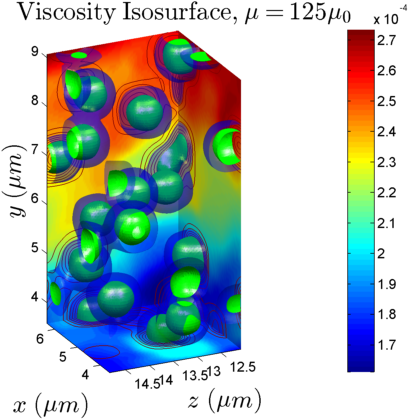
(a)

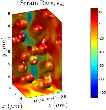
(b)

Figure 3: a) A viscosity isosurface is shown for a small section of a biofilm used in simulation. The inner isosurface is $\mu=125\mu_{0}$ and the outer transparent isosurface is at $\mu=50\mu_{0}$. Slices of the $||\mathbf{u}||$ velocity field are shown as well. b) The $\dot{\epsilon}_{yz}$ component of the strain rate is plotted on the $\mu=125\mu_{0}$ viscosity isosurface. Additionally, the strain rate and contours of viscosity are shown in slice planes. For a single phase fluid, Newton’s viscosity law is $\sigma=\mu\dot{\epsilon}$. Although biofilms are not Newtonian fluids, we still see that in areas of low viscosity, higher strain rates are found and in areas of higher viscosity lower strain rates occur.

3.2 Numerical Verification and Convergence Properties

In the first numerical verification result, we verify the accuracy of the numerical projection method solver with no biofilm present by comparing the numerical solution with an analytical solution. Since there is no immersed structure, this is a test of the fluid solver alone, and not the IBM method. For this test, the domain, $\Omega$ is chosen to be a rectangular solid that is periodic in the $x$ and $z$ directions. From [7], the following boundary conditions for $y=0$ and $y_{L}$,

$$\frac{\partial P}{\partial y}=0\quad \mathbf{u}|_{0}=\mathbf{0}\quad\mathbf{u}|_{y_{L}} =\langle 0,\,0,\,\sin\nu t\rangle$$ (15)

provide us with an analytic solution,

$$u_{z}(y,\,t)=\left|\frac{\sinh k\,y(1+i)}{\sinh k\,y_{L}(1+i)}\right|\sin\left(\nu\,t+\arg\left(\frac{\sinh k\,y(1+i)}{\sinh k\,y_{L}(1+i)}\right)\right)\,\,\,\,\,k=\left(\frac{\nu\rho}{2\mu}\right)^{1/2}.$$ (16)

The values of $P$, $u_{x}$ and $u_{y}$ are exactly zero in this case. The values of $\rho$ and $\mu$ are set to $998\,\mathrm{kg}/m^{3}$and $1\,\mathrm{Pa}\cdot s$ respectively and are homogenous across the domain since no analytic solutions with variable density and viscosity and the boundary conditions given above are known to the authors. Convergence tests were conducted with frequencies $\nu=1\,Hz$ and $\nu=100\,Hz$. In Table 3 the absolute error, temporal convergence factors, and spatial convergence factors are listed. These quantities are calculated as described in Part I [15].

Frequency	Time	Space	Error $||\mathbf{u}^{h}-\mathbf{u}||_{\infty}$
$1\,Hz$	1.006	1.801	$4.910\cdot 10^{-10}$
$100\,Hz$	1.221	2.002	$2.223\cdot 10^{-5}$

Table 3: Spatial convergence tests were carried out with grid spacings, $h$, set to 1/32, 1/64, and 1/128 and a time step of $\Delta t=1/500/\nu$. Temporal convergence tests were done with $\nu\Delta t$ set to 1/125, 1/250, and 1/500 and $\Delta x=1/64$. Error is computed at $t=(0.2/\nu)\,s$. Convergence factors are computed as $\rho(\Delta t)=\log\frac{||u(\Delta t/2)-u(\Delta t)||_{2}}{||u(\Delta t/4)-u(\Delta t/2)||_{2}}$ in time and by $\rho(h)=\log\frac{||u(h/2)-I_{h}^{h/2}u(h)||_{2}}{||u(h/4)-I_{h/2}^{h/4}u(h)/2||_{2}}$ where $I_{h}^{h/2}$ is an interpolation operator taking functions from a grid with spacing $h$ to a grid with spacing $h/2$.

Additionally, with the same boundary conditions as above, we tested the convergence rates for simulations with a biofilm that possesses variable density and viscosity. Temporal and spatial convergence factors are shown in Table 4. More detailed numerical convergence results for this model with different boundary conditions are shown in [15]. In Table 4, temporal convergence factors for the same fluid conditions and domain as the analytical solution are listed. The pressure convergence rate is not shown here since pressure variation only varies by about $\mathcal{O}(10^{-5})$ and thus is around the same order as the numerical errors observed in the finite difference approximations used.

Frequency	Velocity, $||\mathbf{u}||$		Position, $||\mathbf{X}||$
	Time	Space	Time	Space
$49.91\,Hz$	0.983	1.105	1.022	0.952
$4.991\,Hz$	0.991	0.910	1.007	1.054

Table 4: Convergence factors of hrIBM with biofilm. For spatial convergence, $h$ was set to 1/32, 1/64, and 1/128 with a time step of $\nu\Delta t=1/500$. To measure the temporal convergence factors, $\nu\Delta t$ was set to 1/250, 1/500, and 1/1000. In both cases, the boundary conditions described in Section 3 were used.

4 Experimental Validation Results

The material characterization of bacterial biofilms is a difficult experimental task. It is usually not possible to grow biofilms large enough for use in standard testing devices and, attempts to move a biofilm from the environment it was grown in to a testing apparatus may alter its structure [22]. In Pavlovsky et al. (2013) [22], a promising experimental method of testing material properties of biofilms was developed. In the experimental setup, a biofilm is grown in a parallel plate rheometer. As the biofilm grows, it adheres to both the top and bottom plate of the device. The top plate can then be rotated or repositioned vertically and the stress and strain induced in the biofilm can be monitered. These measurements can then be used to infer material properties of the biofilm. Using the hrIBM model, we set up a simulation to reproduce experiments described in Pavlovsky et al (2013).

In order to reproduce the biofilm in simulation, 3D position data sets obtained by high resolution microscopy of live biofilms are used to initialize the positions of bacteria in the computational domain. The experimental setup used to obtain these data sets are described in Pavlovsky et al. (2015) [21] and Stewart et al. [25]. Although the biofilm position data sets that we use, which were obtained from the experiments described in [21], are not the ones grown and tested in the bioreactor, they are from biofilms grown under similar physical and nutrient availability conditions. A key result seen from our simulations is that the material properties computed by our model of the different data sets are similar to each other. This indicates that the material properties obtained through simulation must depend on larger scale structural properties of the biofilm and may be treated as bulk properties of the biofilm. For validation we compared bulk properties measured by our model to experimental results. The methods used to compute these quantities are discussed in the next subsections.

In Pavlovsky et al. (2013) [22], small amplitude rheometry (SAR) is used to characterize the viscoelastic behavior of S. epidermidis biofilms. In SAR experiments, the upper plate of the rheometer is rotated to induce a sinusoidal shear deformation such that the average strain amplitude at the top of the biofilm is a fixed value and the corresponding stress is measured. The strain amplitude was set to $0.13$ at the outer radius of the rheometer since this strain amplitude is found to be in a regime of primarily linear and elastic mechanical behavior [22]. Using 23, the dynamic moduli are computed at a number of different frequencies of oscillation.

Creep compliance testing is another characterization technique used in Pavlovsky et al. (2013). In a creep compliance test, a constant shear stress is applied to the biofilm through the top plate of the rheometer. This induces a time dependent strain which can be measured.

With the hrIBM model, we assume that for a small rectangular sample of the biofilm that is not near the rotational center and, does not border the outer boundary of the disc, the effects of cylindrical geometry are negligible and the rotational motion can be approximated as linear shear. This assumption greatly reduces the computational expense of simulating the biofilm and simplifies the discretization of the computational domain. This approximation is valid since the stresses due to angular momentum are much less than those due to the shearing motion of the plates. The size of the bioreactor used experimentally is $40\,mm$ in diameter and approximately $250\,\mu m$ in height, whereas, the computational domain is only $9-18\,\mu m$ in width and length and $18-27\,\mu m$ in height.

From Christensen [8], the shear stress and strain, $\sigma_{\theta z}$ and $\epsilon_{\theta z}$, of an isotropic viscoelastic cylinder undergoing small angle torsion are proportional to $r$, the radial coordinate. Thus, if we choose to simulate some subset of the bioreactor that is $30\,\mu m$ in width (this is larger than in simulations we conduct) that is near, but not touching the outer edge of the cylinder, at a radius of $15\,mm$ from the center, the ratio of shear strain and shear stress exerted at the inner and outer boundaries is approximately $(15\,mm)/(15\,mm+30\,\mu m)=0.998$. Additionally, we see that in this case, the shear strain and shear stress are not functions of the angular coordinate, thus approximating the slightly curved domain as a rectangular solid should not alter the physics of the problem. Of course, biofilms have far more complicated material properties, however, at the scale of our simulations, this result indicates that rectangular geometry and linear shear produces an accurate approximation of the motion of the biofilm..

4.1 Computation of Rheological Properties

In order to compute the desired dynamic moduli, and compliance modulus results, the stress and strain experienced by the biofilm during simulation must be computed. The stress $\boldsymbol{\sigma}$, is decomposed into a sum of stress due to the fluid motion, $\boldsymbol{\sigma}^{f}$, and stress due to the straining of inter-bacteria connections within the biofilm $\boldsymbol{\sigma}^{b}$. The total stress can then be found as $\boldsymbol{\sigma}=\boldsymbol{\sigma}^{b}+\boldsymbol{\sigma}^{f}.$ Although each component of stress is computed separately during simulations, distinct simulations cannot be used to individually test $\boldsymbol{\sigma}^{b}$ and $\boldsymbol{\sigma}^{f}$ since they are coupled.

In order to calucate the strain $\boldsymbol{\epsilon},$ a set of tracer particles is tracked throughout the simulation. Spatial derivatives can then be calculated to obtain approximations of the strain. Additionally, since only small amplitude strains are observed, the linear relation, $\boldsymbol{\epsilon}=\frac{1}{2}(\nabla\mathbf{d}+\nabla^{T}\mathbf{d})$ is an accurate approximation of the strain for a displacement vector $\mathbf{d}$. The derivatives needed to compute the strain are taken with respect to the advected material coordinates.

Viscoelastic materials are often characterized through their time dependent stress response to strain or their time dependent strain response to stress. For a general viscoelastic material, given that the stress and strain are sufficiently smooth functions of time, constitutive relations between the stress and strain may be written in terms of a convolution with viscoelasticity tensors as:

$$\sigma_{ij}(\mathbf{x},\,t)=\int_{-\infty}^{t}G_{ijkl}(\mathbf{x},\thinspace t-\tau)\,\frac{d}{d\tau}\epsilon_{kl}(\mathbf{x},\,\tau)\thinspace d\tau$$ (17)

$$\epsilon_{ij}(\mathbf{x},\,t)=\int_{-\infty}^{t}J_{ijkl}(\mathbf{x},\,t-\tau)\,\frac{d}{d\tau}\sigma_{kl}(\mathbf{x},\,\tau)\,d\tau$$ (18)

where $\sigma_{ij}$ is the stress tensor, $\epsilon_{ij}$ is the strain tensor, and $G_{ijkl}$ and $J_{ijkl}$ are fourth order viscoelasticity tensors (see Christenson [8] , §1 for a derivation). In the literature, $\boldsymbol{G}$ is often called the relaxation modulus and $\boldsymbol{J}$ is called the compliance modulus. For linear, isotropic materials, the expression for $G{}_{ijkl}$ simplifies to $G_{ijkl}=\frac{1}{3}\left(G_{1}(t)-G_{2}(t)\right)\hat{\delta}_{ij}\hat{\delta}_{kl}+\frac{1}{2}G_{1}\left(\hat{\delta}_{ik}\hat{\delta}_{jl}+\hat{\delta}_{il}\hat{\delta}_{jk}\right)$, where $\hat{\delta}_{mn}$ is the Kronecker delta function and Einstein summation notation is used. The two functions, $G_{1}(t)$ and $G_{2}(t)$ correspond respectively to shear and dilatational stresses. Analogous expressions exist for the compliance tensor. Although the viscoelastic moduli are spatially heterogeneous, we believe that more meaningful results are obtained in the mean field, or spatially averaged, time dependent values for $\boldsymbol{\epsilon}$, $\boldsymbol{\sigma}$, $\boldsymbol{G}$, and $\boldsymbol{J}$. These quantities depend less on the exact configuration of bacteria in a biofilm and behave more like bulk material parameters that can be measured experimentally. Although the interconnected links used to model the connections between adjacent bacteria each individually introduce anistropy into the model, under the conditions of our simulations, the overall behavior of the biofilm is not highly anisotropic.

4.1.1 Computation of Strain

Although a single phase Newtonian fluid will behave viscously (i.e., the stress only depends on the strain rate, not strain itself), in a biofilm the fluid component is influenced by the elastic components of the biofilm and thus the stress state in a biofilm depends directly on the strain (along with the strain rate). In order to compute the strain, the displacement field must be computed. The displacement, $\mathbf{d}$ of a particle located at $\mathbf{x}_{0}$ at time, $t=0$ in a material undergoing deformation can be found by solving the following ODE:

$$\frac{\partial}{\partial t}\mathbf{d}(\mathbf{x}_{0},\,t)=\int_{\Omega}\mathbf{u}(\mathbf{x},\,t)\delta(\mathbf{x}-\mathbf{d}(\mathbf{x}_{0},\,t)-\mathbf{x}_{0})\,d\mathbf{x};\quad\mathbf{d}(\mathbf{x}_{0},\,0)=\mathbf{0}.$$ (19)

In the biofilm simulations, “tracer” particles with positions denoted by $\mathbf{S}(x,\,y,\,z)$, are initialized at heights $y_{L}-\gamma$, $y_{L}-\gamma-h$, and $y_{L}-\gamma-2h$, near the top of the biofilm at $t=0.$ At each time step, the positions of the tracers are updated using the same $\delta$ function interpolation used to update the bacteria positions. With these tracers, the deformation of the biofilm can be tracked throughout the simulation.

In the simulations, the $\epsilon_{yz}$ component of strain is needed at the upper boundary of the domain. Therefore, the tracers are initialized near the top of the domain in three vertically aligned layers. This is done to make the numerical approximation of derivatives of the form $\partial d_{z}/\partial y$ easier . With the initial arrangement of tracters in vertically aligned layers, the centered finite difference approximation

$$\epsilon_{yz}(\mathbf{S},\,t)\approx\frac{1}{2}\left(\frac{\partial d_{z}}{\partial y}+\frac{\partial d_{y}}{\partial z}\right)\approx\frac{1}{2}\left(\frac{\partial d_{z}}{\partial y}\right)\approx\frac{1}{2}\left(\frac{1}{2}\frac{d_{z}(\mathbf{S}(y)-d_{z}(\mathbf{S}(y-h))}{S_{y}(y)-S_{y}(y-h)}+\frac{1}{2}\frac{d_{z}(\mathbf{S}(y+h)-d_{z}(\mathbf{S}(y))}{S_{y}(y+h)-S_{y}(y)}\right)$$ (20)

can be used to approximate the strain. The reported value of $\epsilon_{yz}$ at each time step is then the average of the strains calculated over each tuple of tracers. Since the entire upper plate moves at a single velocity at any given time, $\partial d_{y}/\partial z$ is negligible in this case, whereas in general, this term is required to compute the shear strain.

4.1.2 Computation of Stress Induced by Fluid Motion

From Newton’s viscosity law the $\sigma_{yz}^{f}$ component of stress can be found as

$$\sigma_{yz}^{f}=\mu(\mathbf{x})\left(\frac{\partial u_{z}}{\partial y}+\frac{\partial u_{y}}{\partial z}\right).$$ (21)

Since the velocity field is already known from solving the Navier-Stokes equations at each time step, the relevant derivatives can be approximated by finite difference approximations. As with the strain calculation, the second term, $\partial u_{y}/\partial z$, is zero since the $y$ velocity on the entire top plate of the rheometer is zero. The reported value of $\sigma_{yz}^{f}$ at each time step is then found by spatially averaging over the top $2.5\,\mu m$ of the domain. This is done instead of just averaging over the very top of the domain in case there are numerical boundary layers in the fluid flow field near the boundary. Boundary layers of thickness $\mathcal{O}(\sqrt{\mu\Delta t/\rho})$ are known to sometimes arise in projection method based fluid solvers [5, 20].To mitigate this problem, we use boundary conditions that do not cause this issue in the constant density and viscosity case.

4.1.3 Computation of Stress Induced by the Biofilm Configuration

In order to compute the force exerted by the biofilm connections on the top plate, we integrate the Eulerian force field induced by bacteria adhered to the top plate. To determine if a bacteria is adhered, we choose a distance, $\gamma=0.4\,\mu m$ from the top plate, and assume that each bacteria with $y$ coordinate in the interval $[y_{L}-\gamma,\,y_{L}]$ is adhered to the top, and that its $z$-component of velocity is fixed to be that of the upper plate. For these bacteria, any force applied on them by spring-like connections to other bacteria behaves like a force exerted by the biofilm on the upper plate instead of on the bulk fluid. The sum of these forces is used to compute the stress induced by the spring-like connections by means of Cauchy’s traction law,

$$\boldsymbol{\sigma}^{b}\mathbf{n}=\frac{\mathbf{F}^{b}}{A}.$$ (22)

The outward unit normal, $\mathbf{n}$, is $(0,\,1,\,0)$ in this case since the top plate is parallel to the $xz$ plane. The force, $\mathbf{F}^{b}$ is found by integrating the Eulerian force density field that would be generated by the biofilm nodes adhered to the top plate. Additionally, since we are interested in the applied shear stress, $\sigma_{zy}^{b}$, this can be found as -$\frac{F_{z}^{b}}{A}$. Note that $\gamma$ was chosen arbitrarily, however we observed that with $\gamma=0.7\,\mu m$ the results were not significantly different.

4.2 Shear Moduli, $G^{\prime}$and $G^{\prime\prime}$

When a nearly isotropic material is subjected to an oscillatory displacement field with frequency $\nu$, we may write the strain as $\epsilon(t)=i\nu\thinspace\epsilon_{0}e^{i\nu t}$, where $i$ is the imaginary unit and $\epsilon_{0}$ is the strain amplitude. For cases where the strain is primarily only shear strain equation (17) gives, $\boldsymbol{\sigma}(\nu)\approx G_{1}^{\ast}(\nu)\boldsymbol{\epsilon}(\nu)$ where $G_{1}^{\ast}(\nu$) is related to the Fourier transform in time of $G_{1}(t)$. In general $G_{1}^{\ast}(\nu)$ is a complex valued function. Breaking the complex shear modulus into its real and imaginary components, $G_{1}^{\ast}(\nu)=G^{\prime}(\nu)+iG^{\prime\prime}(\nu)$; and given a strain amplitude $\epsilon_{0}(\nu)$ and stress amplitude $\sigma_{0}(\nu)$ (in Pascals),

$$G^{\prime}(\nu)=\frac{\sigma_{0}(\nu)}{\epsilon_{0}(\nu)}\cos\delta(\nu),\qquad G^{\prime\prime}(\nu)=\frac{\sigma_{0}(\nu)}{\epsilon_{0}(\nu)}\sin\delta(\nu).$$ (23)

Here, $\delta(\nu)$ is known as the loss angle, measured in radians at frequency $\nu$. In the literature, $G^{\prime}(\nu)$ and $G^{\prime\prime}(\nu)$ are often referred to as the storage and loss moduli. They correspond to the elastic and viscous components of a viscoelastic stress strain relationship.

Taking the domain to be a rectangular solid, oriented as shown in Figure 2, we assume that all fields are periodic in the $x$ and $z$ directions. We use the following boundary conditions:

$$\begin{array}[]{ccc}\left.\frac{\partial P}{\partial y}\right|_{y=0,y_{L}}=0&\mathbf{u}(x,0,z,t)=0&\mathbf{u}(x,y_{L},z,t)=(0\>,0\>,u_{b}(t)\,).\end{array}$$ (24)

Along the top boundary, we set the $z$ velocity to be

$$u_{b}(t)=\epsilon_{0}\frac{(e^{2\nu t}-1)((e^{4\nu t}-1)\cos\nu t+8e^{2\nu t}\sin\nu t)}{(1+e^{2\nu t})^{3}}.$$ (25)

This particular function is chosen since it is continuous, at $t=0$, $u_{z}=0$, and because it converges to within 0.001 of $\epsilon_{0}\cos\nu t$ within half an oscillation, reducing the amount of time needed to run simulations. To initialize the bacteria positions, we take a $9\,\mu m\times 27\,\mu m\times 9\,\mu m$ subset of a $30\,\mu m\times 30\,\mu m\times 10\,\mu m$ bacteria position data field obtained experimentally. This data is also used in the initialization of the viscosity and density fields present in the biofilm. We believe that setting the internal forces to zero at the start is reasonable since experimental results from SAR under both compression and tension yielded similar results. In Figure 4, the deformation induced by an oscillatory shearing motion is depicted.

Figure 4: Starting at $t=0$ on the left, the images show how the biofilm is moved as the top plate oscillates. Dots are bacteria locations and lines indicate viscoelastic connections. In the simulations the domain is periodic in the $x$ and $z$ directions. The periodicity is not shown here since it makes it more difficult to visualize the effect of deformation on the biofilm.

In order to tune our model to the experimental data, we adjusted the spring constant, $k_{ij}$ used in Hooke’s Law and the distance by which we allow any two biofilm nodes to be connected by at time $t=0$. For a spring connecting two points in space, Hooke’s Law can be written as

$$\mathbf{F}_{ij}=k_{ij}\,\Lambda_{ij}(\mathbf{X},\,\mathbf{X}_{0})\,(\mathbf{X}_{i}-\mathbf{X}_{j}),$$ (26)

with

$$\Lambda_{ij}(\mathbf{X},\,\mathbf{X}_{0})=\frac{||\mathbf{X}_{i}(t)-\mathbf{X}_{j}(t)||-||\mathbf{X}_{i}(0)-\mathbf{X}_{j}(0)||}{||\mathbf{X}_{i}(t)-\mathbf{X}_{j}(t)||}.$$ (27)

Following Hammond et al. [15], we choose each $k_{ij}$ to be a force constant, $F_{max}$ divided by the initial separation of bacteria $i$ and $j$. Since the immersed boundary method requires a Lagrangian force density, we then divide $\mathbf{F}_{ij}$ by the Lagrangian volume element, $d_{0}^{3}$. Additionally, we note that in Dan Vo et al. [9] and Peskin [24], an identical constitutive relation is derived from the starting point of energy functionals in which the force density is found by taking a Fréchet derivative of an energy functional.

In Figure 5 we depict the frequency dependence of $G^{\prime}$ and $G^{\prime\prime}$ . From these results, it is clear that our model fits experimental data on $G^{\prime}$ quite well. For $G^{\prime\prime}$ the fit is not as strong, although we still do see that many of the results from simulation are within the range of experimental error. We observe that in fact the slope of $G^{\prime\prime}$ is steeper than the experimental measurements. Although at this time, the cause of this difference is unknown, it is possible that extensions such as those discussed in Section 5 may correct this.

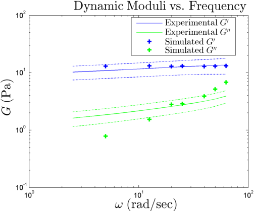
Figure 5: A comparison between experimentally measured results for $G^{\prime}$ and $G^{\prime\prime}$ is shown in comparison the simulation results. For these results, the force constant was $F_{max}=1.3223\cdot 10^{-9}$ , the connection distance between bacteria was $1.62\mu m$, no damping was used, $\mu_{b}=250\mu_{0}$, and $\rho_{b}=1.12\rho_{0}$. The dashed lines indicate the experimental error range.

4.3 Creep Compliance Measurements $J(t)$

Creep compliance is a measure of how a material deforms over time in response to an applied stress. Experimentally, the compliance is measured by using the rheometer to apply a step change to the shear stress on the upper plate and observing the resultant shear strain. A step change in stress can be written as, $\bar{\sigma}(t)=\sigma_{0}H(t)$ where $\sigma_{0}$ is the magnitude of the step change and, $H(t)$ is the Heaviside step function. For a linear isotropic material with $\sigma_{yz}(t)=\bar{\sigma}(t)$, the integral in Equation (18) simplifies to

$$\epsilon_{yz}(t)=\sigma_{0}J_{1}(t).$$ (28)

From a physical standpoint, most of the bacteria and the bulk of the fluid are only effected by the step change in stress after the stress propogates vertically through the biofilm. However, in the portion of the biofilm adjacent to the upper plate the effect of a change in stress is instantaneous. Thus, we can write a force balance between the forces in the biofilm, the acceleration of the top plate, and the applied force on the top plate. This leads to an impulse boundary condition which specifies the velocity at the top plate The boundary condition can be written as

$$\left.\frac{d}{dt}u_{z}\right|_{y=H}=(\rho V)^{-1}(\sigma_{0}-\sigma^{b}-\sigma^{f})A$$ (29)

where $\sigma^{b}$ and $\sigma^{f}$ are the stress exerted by the fluid and the springs in the biofilm at the top plate, $A$ is the area of the upper plate, and $(\rho V)$ is the mass associated with the top plate of the rheometer. We assume that this mass is equivalent to the mass of the top $2.4\,\mu m$ of the biofilm where bacteria are adhered to the top plate.

Numerically, this boundary condition can be written as

$$u_{z}^{(n+1)}|_{y=H}=u_{z}^{(n)}|_{y=H}+\left(\frac{\Delta t}{\rho_{0}u_{0}L\sum_{\mathcal{G}_{h}}\rho_{ijk}}\right)(\sigma_{0}-\sigma^{b}-\sigma^{f}).$$ (30)

In (30), $\rho_{0}$ and $\mu_{0}$ are the density and viscosity of water, and $L$ is the characteristic length (in this case $10\,\mu m$). In numerical experiments, rather than immediately impose a step in stress at time 0, we add a mollifier, $\left(\frac{2}{1-e^{-\alpha t}}-1\right)$ on the applied stress, $\sigma_{0}$ to mitigate any possible numerical instabilities associated with a discontinuous boundary condition. In this case, $\alpha=200$ is chosen to be large so that the applied stress approaches its equilibrium value within 0.1 seconds. This is reasonable because very short time compliance behavior is not generally experimentally measurable, and also a step in the stress may not actually occur instantaneously from the perspective of a very short time scale. Results from simulations using this boundary condition andtwo values of $\sigma_{0}$ are shown in Figure 6.

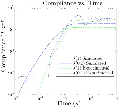
Figure 6: The time dependence of $J(t,\,\sigma_{0})$ is shown above for $\sigma_{0}=0.1\,Pa$ and $\sigma_{0}=1\,Pa$. It can be seen that the compliance levels out at a similar value as the experimental result, but levels out faster than in the experiments. For the compliance simulations, we used $F_{max}=2.9091\cdot 10^{-9}$ instead of $F_{max}=1.3223\cdot 10^{-9}$ due to some numerical stability issues.

Presently, we do not propose mechanisms by which the spring-like connections may break and reconnect, although it is possible to incorporate such a model into our current framework as discussed in [15]. Thus, the long term behavior of $J_{1}(t,\,\sigma_{0})$ which likely depends on the gradual redistribution of the connectivity of the biofilm is not expected to be captured. Therefore, we do not simulate beyond 0.1 seconds. In the experimental results, there are some damped oscillations present in the creep compliance experiments. In Pavlovsky et al. (2013), these oscillations are found to be related to intertial effects from the rheometer itself and thus are not expected or observed in our simulations.

4.4 Similarity of Material Properties Between Different Bacteria Position Data Sets

In Dzul et al. [10], the spatial statistics of bacteria in a biofilm are studied. We show here that from data sets that have similar spatial distributions of nearest neighbor connections between bacteria, similar bulk property measurements are obtained. In our simulations, we take blocks of experimental data that are $18\,\mu m$ wide, $9\,\mu m$ long, and $27\,\mu m$ high and compute the dynamic moduli of each block at a fixed frequency. . The graphs in Figure 7 show the stress and strain of four different biofilms over one period of oscillation.

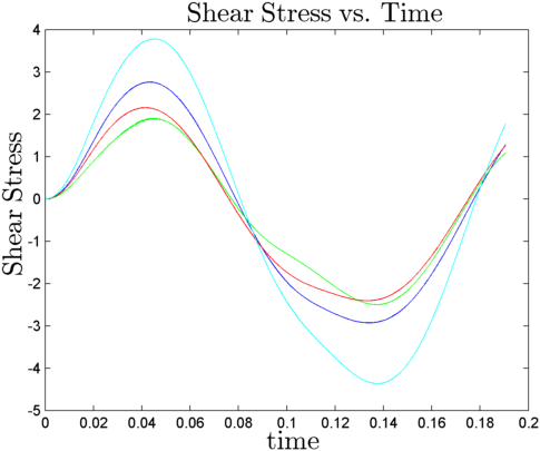
(a)

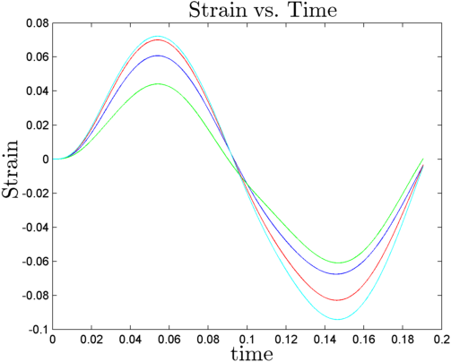
(b)

Figure 7: These graphs show the stress vs. time and strain vs. time for 4 different biofilm samples. The samples are all $18\mu m\times 27\mu m\times 9\mu m$ size and contain approximately 2000 bacteria positions.

From figure 7 and Table 5, we see that in three of the four biofilm data sets, similar results are obtained.. We also note that the mean standard error in the experimental results for this particular test was 3.9791 for $G^{\prime}$ and 0.8836 for $G^{\prime\prime}$. We also suspect that if larger data sets were used, even better agreement would be seen in the computed values of $G^{\prime}$ and $G^{\prime\prime}$.

The importance of this section is in verifying that the properties we are validating can be considered as bulk properties. Since three out of the four data sets provided results within the experimental error deviation, we believe this to be strong evidence the properties we measure are bulk properties.

Simulation	1	2	3
$G^{\prime}(\nu=49.91)$	13.06	9.18	10.03
$G^{\prime\prime}(\nu=49.91)$	-5.16	-4.44	-3.92
$\delta(\nu=49.91)$	0.376	0.451	0.373

Table 5: Results for $G^{\prime}(\nu)$, $G^{\prime\prime}(\nu)$ and $\delta(\nu)$ are shown at two frequencies for 3 different biofilm coordinate data sets with $\nu=49.91\,rad/s$. These results show that the physical properties measured here do not depend solely on the exact microstructure of the biofilm, but on sometype of more large scale organization of the bacteria positions in space.

4.5 In-Stream Tumbling of Biofilm Fragment

Bacterial structures exhibit a diverse range of interaction with fluid flow. One such interaction is the tumbling motion of aggregates in shear flow. To simulate this effect, we conduct simulations in which there are no bacteria anchored along the plates of the domain. Instead, an aggregate of bacteria is located near the middle of the computational domain and the upper and lower plates move in opposite directions as

$$u_{z}(x,\,y_{L},\,z)=10^{-3}\left(\frac{1}{1+e^{-t}}-\frac{1}{2}\right)=-u_{z}(x,\,0,\,z).$$ (31)

The boundary velocities are scaled by $10^{-3}$ so as to limit the shear stress so that the aggregate is not simply torn apart. To ensure that the biofilm is not attached to the plates and is sufficiently far from the plate to induce a rotating, or tumbling motion, these simulations only include bacteria that are greater than $8.8\,\mu m$ from either plate at the start. With the physical parameters we use, the bacteria aggregation rotates and is deformed by the fluid shear forces exerted by the fluid [6].

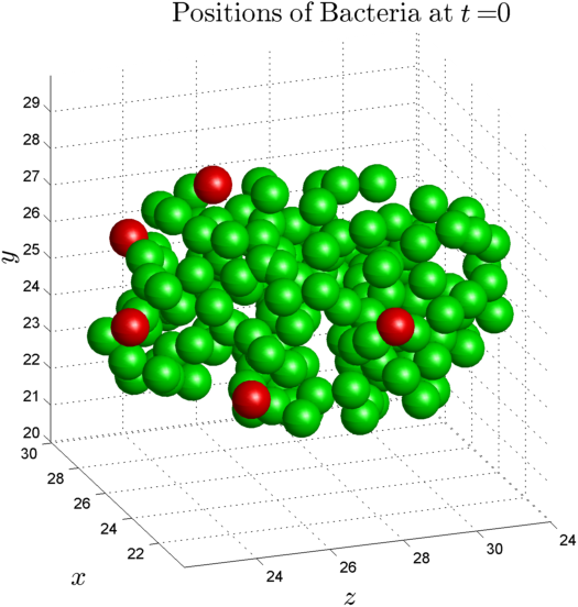
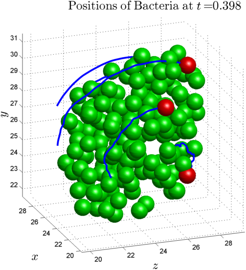
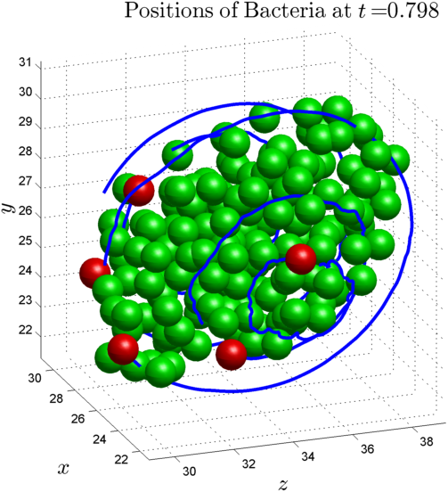
Figure 8: Biofilm aggregate suspended in shear flow rotate over time. Snap shots shown at 0, 0.4 and 0.8 seconds into the simulation. The flattening of the ellipse in response to the shear flow can be distinguished between the first and third figure. Several bacteria are marked red to help show the rotation of the aggregate. The blue lines indicates the trajectories of the marked cells relative to the center of mass of the aggregate. Distances are in 10s of micrometers.

In Blaser et al. [3], analytical results on the frequency at which a solid ellipsoid will rotate in shear flow are provided. For an ellipsoid with axis aligned with the direction of fluid motion, the rotational frequency is found as

$$T=\frac{2\pi(a_{1}^{2}+a_{2}^{2})}{a_{1}a_{2}\tau}$$

where $\tau$ is the shear rate and $a_{1}$and $a_{2}$ are the principle axes of the ellipse undergoing rotation. In our simulation (see Figure 8), we show that a bacterial aggregate approximated as a hydrodynamically equivalent ellipse will rotate at a frequency similar to the theoretically expected result. The rotational frequency of the aggregate is found by computing the average frequency of rotation of bacteria in the $yz$ plane about the center of mass of the aggregate. In the simulations, we observed a frequency of approximately 0.76 seconds for an aggregate approximated by an ellipse with major axis $a_{1}=0.167\,\mu m$ and first semimajor axis $a_{2}=0.136$, and with shear rate of $20\,s^{-1}$ containing 54 bacteria. The theoretical result in this case is 0.641 seconds. These results are shown in Table 6. Although in our case these results are not as concrete of a metric as the dynamic modulus and compliance results, rotational frequency has been used for model validation in fields such as red blood cell modeling (see [11]).

Major axis, $a_{1}$	First minor axis, $a_{2}$	Theoretical Period	Observed Period	Relative Error
$1.67\mu m$	$1.36\mu m$	$0.64s$	$0.76s$	$+18.8\%$
$4.94\mu m$	$2.74\mu m$	$0.59s$	$0.67s$	$+13.5\%$

Table 6: Comparison of theoretical and simulated rotational results

5 Discussion and Future Directions

Although we see that the hrIBM model provides a versatile means of simulating biofilms and can accurately capture some of the experimentally observed behavior of biofilms, there is still room to extend the model to allow for more general modeling of biofilms. An important area of research in biofilm studies is developing an understanding of the fracture mechanics and dynamics of biofilms. One way to model fracture dynamics in our biofilm model would be the inclusion of a stochastic model governing the connectivity of the viscoelastic links in the biofilm. Thus, we could define a probability based on the stress and strain in each link and the proximity of each pair of connected bacteria to allow for reconfiguration of the connectivity of the biofilm over time. It is also possible to model the viscoelastic properties of the biofilm by adjusting the constitutive model that is used to provide the Lagrangian force based on the nodal configuration of the bacteria. Modeling the changing connectivity of a biofilm was explored in [2, 4, 26].

Another area that could be explored is the shape of the discrete $\delta$ function used to approximate each bacteria and its associated viscosity halo. It is possible that adjusting this function may allow for more accurate modeling of the mass displacement induced by the bacteria bodies in the bulk fluid. Adjustments to the $\delta$ function may also allow for the inclusion of nonspherical bacteria into the model. It would be interesting to see if similar results are obtained for bacteria that are different shapes.

One possible difficulty in adjusting the discrete $\delta$ function is the preservation of mass in the model. In Equation (2), there is no density dependence as would normally be seen with the Navier-Stokes equations for a variable density system. For the original IBM, this is in fact exact as described in [24]. For the hrIBM, there is an error however, error term is expected to be small in our situation since $\rho(\mathbf{x},\,t$) only varies by $12\%$ over the domain (density of bacteria is not highly variable), all simulations are at low Reynold’s numbers, and the high viscosity gradients which overlap where density gradients occur make it difficult for fluid to rapidly travel down a density gradient. Although we believe that this approximation is accurate in the simulations we conduct, this error term may increase in situations with higher Reynold’s numbers. This is an area that may be further developed in future works.

Another area of potential improvement is the numerical methods. Currently the scheme is $\mathcal{O}(\Delta t$) and $\mathcal{O}(h$). In future work, the Crank-Nicholson time-stepping scheme may be used since, at least in the constant viscosity and density case, it could lead to $\mathcal{O}(\Delta t^{2})$ convergence as shown in Brown et al. [5]. Another approach is to use a predictor-corrector type of method such as those described in [11] and [24]. However, even without heterogeneous material properties, obtaining $\mathcal{O}(\Delta t^{2})$ convergence in the overall IBM is more complicated and also depends on properties of the discrete Dirac $\delta$ function. A detailed discussion can be found in Liu and Mori [17, 18]. The development of efficient $\mathcal{O}(\Delta t^{2})$ IBM schemes with heterogeneous material properties is still an area of active research.

6 Conclusions

Based on the experimental results shown above and in [15], we show that our biofilm model, Equations (1)-(8), can be used to determine bulk material properties of bacterial biofilms. In particular, we show that the model yields close agreement with experimental results from [22] in which the bacterium S. epidermidis was grown in a bioreactor and characterized using a parallel plate rheometer. We also show that suspended aggregates of bacteria in shear flow rotate with a similar period as a hydrodynamically equivalent ellipse. Another development is the uniformity of bulk material properties over different experimental data sets that possess similar spatial statistics. An important step in obtaining these results was the computation of bulk material properties from simulations. To our knowledge, our model is the first that can compute bulk material properties of biofilms based on direct simulation of both microscale connectivity of the biofilm and the heterogeneous rheology of the ECM.

We also acknowledge a number of new research directions and extensions that can be done to improve results and also to allow for more flexible modeling of biofilms in different scenarios than what we have considered here.

7 Acknowledgements

This work was supported by the National Science Foundation grants PHY-0940991 and DMS-1225878 to DMB, and PHY-0941227 to JGY and MJS, and by the Department of Energy through the Computational Science Graduate Fellowship program, DE-FG02-97ER25308, to JAS. This work utilized the Janus supercomputer, which is supported by the National Science Foundation (award number CNS-0821794), the University of Colorado Boulder, the University of Colorado Denver, and the National Center for Atmospheric Research. The Janus supercomputer is operated by the University of Colorado Boulder.

References

- [1] Erik Alpkvist and Isaac Klapper, A Multidimensional Multispecies Continuum Model for Heterogeneous Biofilm Development, Bulletin of Mathematical Biology, 69 (2007-02-22), pp. 765–789.
- [2] Erik Alpkvist, Cristian Picioreanu, Mark C.M. van Loosdrecht, and Anders Heyden, Three-dimensional biofilm model with individual cells and continuum EPS matrix, Biotechnology and Bioengineering, 94 (2006-08-05), pp. 961–979.
- [3] Stefan Blaser, Forces on the surface of small ellipsoidal particles immersed in a linear flow field, Chemical Engineering Science, 57 (2002-02), pp. 515–526.
- [4] Dean C. Bottino, Modeling Viscoelastic Networks and Cell Deformation in the Context of the Immersed Boundary Method, Journal of Computational Physics, 147 (1998-11), pp. 86–113.
- [5] David L. Brown, Ricardo Cortez, and Michael L. Minion, Accurate projection methods for the incompressible navier-stokes equations, Journal of Computational Physics, 168 (2001-04), pp. 464–499.
- [6] Erin Byrne, Steve Dzul, Michael Solomon, John Younger, and David M. Bortz, Postfragmentation density function for bacterial aggregates in laminar flow, Physical Review E, 83 (2011). bibtex: Byrne2011.
- [7] Horatio S. Carlslaw and John C. Jaegar, Conduction of Heat in Solids, Oxford University Press, 2nd Edition ed., 1959.
- [8] Richard M. Christensen, Theory of Viscoelasticity: An Introduction, Academic Press, 2nd Edition ed., 1982.
- [9] Garret Dan Vo, Eric Brindle, and Jeffrey Heys, An experimentally validated immersed boundary model of fluid-biofilm interaction, Water Science & Technology, 61 (2010-06), p. 3033.
- [10] Stephen P. Dzul, Margaret M. Thornton, Danial N. Hohne, Elizabeth J. Stewart, Aayush A. Shah, David M. Bortz, Michael J. Solomon, and John G. Younger, Contribution of the klebsiella pneumoniae capsule to bacterial aggregate and biofilm microstructures, Applied and Environmental Microbiology, 77 (2011-03-01), pp. 1777–1782.
- [11] Thomas G. Fai, Boyce E. Griffith, Yoichiro Mori, and Charles S. Peskin, Immersed Boundary Method for Variable Viscosity and Variable Density Problems Using Fast Constant-Coefficient Linear Solvers I: Numerical Method and Results, SIAM Journal on Scientific Computing, 35 (2013-01), pp. B1132–B1161.
- [12] , Immersed Boundary Method for Variable Viscosity and Variable Density Problems Using Fast Constant-Coefficient Linear Solvers II: Theory, SIAM Journal on Scientific Computing, 36 (2014-01), pp. B589–B621.
- [13] Timothy Foster, Staphylococcus, in Medical Microbiology, Samuel Baron, ed., University of Texas Medical Branch at Galveston, Galveston (TX), 4th ed., 1996.
- [14] Fabien Gaboriaud, Michelle L. Gee, Richard Strugnell, and Jerome F. L. Duval, Coupled Electrostatic, Hydrodynamic, and Mechanical Properties of Bacterial Interfaces in Aqueous Media, Langmuir, 24 (2008-10-07), pp. 10988–10995.
- [15] Jason F. Hammond, Elizabeth Stewart, John G. Younger, Michael J. Solomon, and David M. Bortz, Variable Viscosity and Density Biofilm Simulations using an Immersed Boundary Method, Part I: Numerical Scheme and Convergence Results, Computer Modeling in Engineering and Sciences, 98 (2014), pp. 295–340.
- [16] C.S. Laspidou, L.A. Spyrou, N. Aravas, and B.E. Rittmann, Material modeling of biofilm mechanical properties, Mathematical Biosciences, 251 (2014-05), pp. 11–15.
- [17] Yang Liu and Yoichiro Mori, Properties of Discrete Delta Functions and Local Convergence of the Immersed Boundary Method, SIAM Journal on Numerical Analysis, 50 (2012-01), pp. 2986–3015.
- [18] , $L^p$ Convergence of the Immersed Boundary Method for Stationary Stokes Problems, SIAM Journal on Numerical Analysis, 52 (2014-01), pp. 496–514.
- [19] Haoxiang Luo, Rajat Mittal, Xudong Zheng, Steven A. Bielamowicz, Raymond J. Walsh, and James K. Hahn, An immersed-boundary method for flow-structure interaction in biological systems with application to phonation, Journal of Computational Physics, 227 (2008-11), pp. 9303–9332.
- [20] Steven A. Orszag, Moshe Israeli, and Michel O. Deville, Boundary conditions for incompressible flows, Journal of Scientific Computing, 1 (1986-03-01), pp. 75–111.
- [21] Leonid Pavlovsky, Rachael A. Sturtevant, John G. Younger, and Michael J. Solomon, Effects of temperature on the morphological, polymeric, and mechanical properties of Staphylococcus epidermidis bacterial biofilms, Langmuir, 31 (2015), pp. 2036–2042.
- [22] Leonid Pavlovsky, John G. Younger, and Michael J. Solomon, In situ rheology of Staphylococcus epidermidis bacterial biofilms, Soft Matter, 9 (2013), p. 122.
- [23] Charles S Peskin, Numerical analysis of blood flow in the heart, Journal of Computational Physics, 25 (1977-11), pp. 220–252.
- [24] Charles S. Peskin, The immersed boundary method, Acta Numerica, 11 (2002-01).
- [25] Elizabeth J. Stewart, Ashley E. Satorius, John G. Younger, and Michael J. Solomon, Role of environmental and antibiotic stress on staphylococcus epidermidis biofilm microstructure, Langmuir, 29 (2013), pp. 7017–7024.
- [26] Rangarajan Sudarsan, Sudeshna Ghosh, John M. Stockie, and Hermann J. Eberl, Simulating biofilm deformation and detachment with the immersed boundary method, arXiv:1501.07221 [physics], (2015-01-28). arXiv: 1501.07221.
- [27] Luoding Zhu and Charles S. Peskin, Interaction of two flapping filaments in a flowing soap film, Physics of Fluids, 15 (2003), p. 1954.
- [28] Jingxuan Zhuo and Robert Dillon, Using the immersed boundary method to model complex fluids-structure interaction in sperm motility, Discrete and Continuous Dynamical Systems - Series B, 15 (2010-12), pp. 343–355.