Extremely Soft X-ray Flash as the indicator of off-axis orphan GRB afterglow

Abstract

We verified the off-axis jet model of X-ray flashes (XRFs) and examined a discovery of off-axis orphan gamma-ray burst (GRBs) afterglows. The XRF sample was selected on the basis of the following three factors: (1) a constraint on the lower peak energy of the prompt spectrum $E^{src}_{obs}$, (2) redshift measurements, and (3) multi-color observations of an earlier (or brightening) phase. XRF020903 was the only sample selected basis of these criteria. A complete optical multi-color afterglow light curve of XRF020903 obtained from archived data and photometric results in literature showed an achromatic brightening around 0.7 days. An off-axis jet model with a large observing angle (0.21 rad, which is twice the jet opening half-angle, $\theta_{jet}$) can naturally describe the achromatic brightening and the prompt X-ray spectral properties. This result indicates the existence of off-axis orphan GRB afterglow light curves. Events with a larger viewing angle ($>\sim 2\theta_{jet}$) could be discovered using an 8-m class telescope with wide field imagers such as Subaru Hyper-Suprime-Cam and the Large Synoptic Survey Telescope.

1. Introduction

Long gamma-ray bursts (GRBs) are believed to occur when a very massive star dies in a highly energetic supernova forming a black hole and producing a relativistic jet. Because of the release of a large amount of isotropic equivalent energy (${\it E}_{\rm iso}\sim 10^{52-55}$ erg) release in the short prompt gamma-ray phase (typically ranging from several seconds to several tens of seconds), the consideration of jet collimation of GRBs is necessary to explain the radiation mechanism from compact sources (e.g., massive stars and/or mergers). This necessity is supported by achromatic temporal breaks (also known as jet breaks) in the afterglow light curves of the GRBs. Ultra-relativistic collimation and a jet structure are required to explain the light curve temporal breaks (e.g., Sari et al., 1999). However, no direct observational evidence exists for this jet collimation.

Off-axis orphan GRB afterglows are produced as a natural consequence of GRB jet production (Rhoads, 1999). The production of these afterglows is as follows: GRBs are collimated with rather narrow opening angles, and the afterglow that follows can be observed over a wider angular range. While the GRB and the early afterglow are collimated to within the original jet opening angle, the afterglow in the late phase can still be observed by an off-axis observer after the jet break. The Lorentz factor, $\Gamma$, is a rapidly decreasing as function of time. This means that an observer at $\theta_{obs}$ cannot see the prompt gamma-ray emissions when $\theta_{obs}>\theta_{jet}$ but can detect an afterglow once $\Gamma^{-1}$ equals $\theta_{obs}$. Here, $\theta_{jet}$ is the jet opening half angle. As the typical emission frequency and flux decrease with time (while the jet opening half angle $\theta_{jet}$ increases with time), observers at larger viewing angles will detect fainter afterglows at longer wavelengths (e.g. optical and radio). Hence, the expected properties of GRB orphan afterglows are as follows: (1) prompt emissions in the high-energy band are absent, (2) their brightness is fainter than that of on-axis GRB optical afterglows, (3) they have the same optical color as on-axis afterglows, and (4) they show host galaxy properties similar to those of on-axis GRBs. The afterglows are characterized by three-component light curves with rising, peaking, and rapidly decaying phases. In this case, events intermediate between classical hard GRBs and off-axis orphan GRB afterglows should exist.

A candidate for the intermediate events is X-ray flashes (XRFs) as Yamazaki et al. (2002, 2003) described in their off-axis jet model for explaining their nature. XRFs were recognized by the Wide Field Cameras (WFC, 2-28 keV; Jager et al., 1997) onboard the BeppoSAX satellite (Heise et al., 2001). The observed X-ray temporal and spectral properties of XRFs in the prompt phase do not show any differences relative to those of GRBs, except for the considerably lower energy values of the peak of the $\nu F_{\nu}$ spectrum in the observer’s frame. A large number of XRF samples were provided by BeppoSAX and High Energy Transient Explorer 2 (HETE-2), both of which employed wide field X-ray cameras $--$ the WFC onboard BeppoSAX and the Wide-Field X-ray Monitor (WXM, 2-25 keV Shirasaki et al., 2003) onboard HETE-2. The majority of HETE-2 samples (nine out of 16 XRFs) show a low energy of spectral peak energy $E^{obs}_{peak}<20$ keV (Sakamoto et al., 2005). The number of XRFs detected by HETE-2 was comparable and relatively larger than that of GRBs indicating that XRFs represent a large portion of the entire GRB population (Sakamoto et al., 2005). The observational properties of XRFs can be interpreted as being associated with the same phenomenon as classical hard GRBs and as being representative of the extension of the GRB population to low peak-energy events (Kippen et al., 2001; Sakamoto et al., 2005). To explain the aforementioned prompt observational properties, three models have been proposed for XRFs: a high redshift origin (Heise, 2003); the off-axis jet model (Yamazaki et al., 2002, 2003; Zhang et al., 2004; Lamb et al., 2005), which is equivalent to the unification scenario of AGN galaxies; and intrinsic properties (e.g., a subenergetic or inefficient fireball), which may also produce on-axis orphan afterglows (Huang et al., 2002).

The Swift satellite has also been detecting many X-ray rich GRBs (XRRs) and XRF samples (Sakamoto et al., 2008). However, the XRF samples tend to be at the high-end of the $E^{obs}_{peak}$ distribution of BeppoSAX and HETE-2. This is because of the relatively higher energy coverage of the Burst Alert Telescope (BAT, 15-150 keV; Barthelmy et al., 2005) onboard Swift. Although the Monitoring of All-sky X-ray Image (MAXI; Matsuoka et al., 2009) attached to the International Space Station has been detecting XRFs (Serino et al., 2014), there has been no appropriate follow-ups because of poor position determination. Hence, XRF studies have stagnated because of the lack of soft-X-ray monitoring instruments and intensive multiwave length follow-up observations.

In this paper, we investigated the characteristics of XRFs on the basis of redshift measurements, multifrequency afterglow monitoring, and spectral peak measurements $E^{src}_{peak}$. The main objective was to verify the off-axis jet model and to provide feedback to ongoing and planned optical untargeted time-domain surveys by using Subaru Hyper-Suprime-Cam (Miyazaki et al., 2012) and the Large Synoptic Survey Telescope (LSST), which have considerable potential for detecting off-axis orphan GRB afterglows.

2. Samples of X-Ray Flash

We considered possible XRFs for our study and quickly realized XRF 020903 was the only event that has (1) either a measurement or an upper bound on the peak energy of the prompt spectrum $E^{src}_{peak}$, (2) a measured redshift, and (3) multicolor afterglow observations adequately cover the early afterglow phase when achromatic brightening of the afterglow might occur. This was one of the XRFs detected by HETE-2 and the first events for which an optical afterglow was detected and a spectroscopic redshift ($z=0.251$) was determined (Soderberg et al., 2004). The prompt emission had the lowest intrinsic spectral peak energy $E^{src}_{peak}$ of $3.3^{+1.8}_{-1.0}$ keV among all the XRF samples. Here, we employed the value estimated by the constrained Band function with the 90% confident level (Sakamoto et al., 2004). In accordance with the report of Sakamoto et al. (2004), the light curve in the prompt phase exhibited a double-peak structure and a lack of signals above 10 keV. Figure 1 shows histograms of the spectral peak energy in the observer frames $E^{obs}_{peak}$ detected by Swift/BAT (Lien et al., 2015), HETE-2 (Sakamoto et al., 2005), the Burst and Transient Source Experiment (BATSE; Kaneko et al., 2006), the Fermi Gamma-ray Burst Monitor (Fermi/GBM; von Kienlin et al., 2014), and Suzaku Wide-Band All-Sky Monitor (WAM). The WAM $E^{obs}_{peak}$ distribution is produced using values, which are available in GCN circulars up to December 2014. The standard analysis procedure of WAM data (Yamaoka et al., 2009) are described in literature (e.g., Ohno et al., 2008; Urata et al., 2012a). For comparison with a large volume of data, we used $E^{obs}_{peak}$ instead of intrinsic spectral peak energies. The lowest intrinsic spectral peak energy determined from the relation $E^{src}_{peak}$=(1+$z$)$E^{obs}_{peak}$ of XRF020903 stands out from all GRB populations. The X-ray to the $\gamma$-ray fluence ratio of 5.6 qualified this burst as an XRF. Here, we used the XRF definition by Sakamoto et al. (2005) for HETE-2 events.

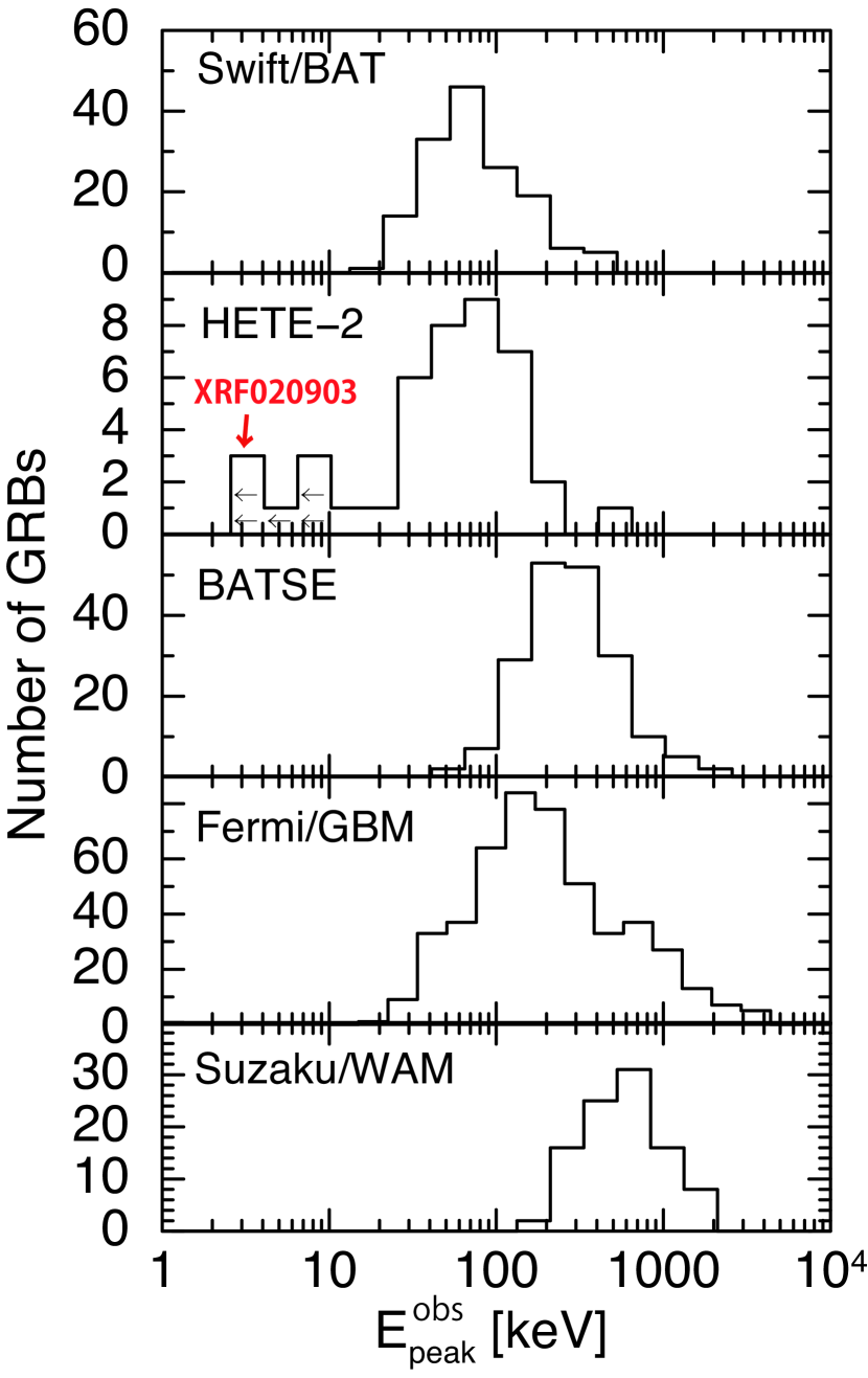
Figure 1.— Distribution of $E^{obs}_{peak}$ for the Swift/BAT, HETE-2, the BATSE, the Fermi/GBM, and the Suzaku/WAM samples. XRF020903 showed the lowest $E^{obs}_{peak}$ among all five samples.

Effective follow-up observations in the optical band were made using wider-field-of-view (FOV) instruments reported by Soderberg et al. (2004) and Bersier et al. (2006). Because of a delay in the position alert and a large position error, the light curve sampling was sparse around the possible rebrightening epoch reported by Bersier et al. (2006). To describe the rebrightening epoch by using multicolor data, we added Subaru archive data, as described in §3.

3. Observations and Data collection

We collected data for the XRF 020903 afterglow by using Subaru archive data and photometric results obtained from literature (Bersier et al., 2006; Soderberg et al., 2004). To perform accurate optical photometry by removing contamination from the host galaxy, we also employed Panoramic Survey Telescope and Rapid Response System 1 (Pan-STARRS1) data. The individual data collections are summarized in the following subsections.

Figure 2.— $Rc/R$, $Ic/I$, and $z$-band images of the XRF020903 field. The first column shows the Subaru images taken in the $Rc$ (top), $Ic$ (middle), and $z$-band (bottom). Reference images for removing the host galaxy component by using the algorithm of Alard & Lupton (1998) are shown in the second column. The top-center, middle-center, and bottom-center panels show the reference images taken with the CTIO $R$-band, CTIO $I$-band and PS1 $z$-band filters. The third column shows $Rc/R$, $Ic/I$, and $z$-band differential images, respectively.

3.1. Subaru Suprime-Cam

The entire HETE-2 position error region was imaged by Suprime-Cam attached to the 8.2-m Subaru telescope. The Suprime-Cam camera consists of ten high-sensitivity 2k$\times$4k CCDs and covers a field of view of $34^{\prime}\times 27^{\prime}$ (Miyazaki et al., 2002). The first epoch of observation on 2002 September 3 (0.16 day after the burst) involved an $Rc$-band filter. Although the observation was performed under marginal airmass conditions (from 2.55 to 2.75), the wide-field imager with the 8-m-class telescope provided the deep $Rc$-band images with three sets of 180 s exposure. Subsequently, three color observations were made on the night of 2002 September 4 by using $Rc-$, $Ic-$, and $z^{\prime}$-band filters. During the night observation, two epochs of $Ic-$ and $z^{\prime}-$ bands imaging and three epochs of $Rc$-band monitoring were also conducted to check the short-term variability of the afterglow. The $Ic-$ and $z^{\prime}-$ band observations were made under the reasonable observing condition (e.g., in the airmass range from 1.34 to 1.97). The second epoch of $Rc$-band imaging was also performed under the reasonable observing condition (e.g., for an airmass of 1.32). By contrast, the first and third epochs of $Rc$-band observations were made under the marginal airmass conditions ($2.65-2.22$ for the first epoch and $1.97-2.27$ for the third epoch). These observations were performed with using appropriate dithering techniques to fill up the chip gaps in the camera.

The Subaru-XMM Deep Survey (SXDS) team attempted to obtain deeper reference images with $Rc$-band filter on the night of October 9 and 10. However, the results were marginal because of poor weather conditions and only two set of images taken with 180 s exposure on 2002 October 9 were available for scientific analysis. Table 1 shows the log of observations for the available images. Because of the limited data set, searching for a counterpart by using only the Suprime-Cam data was difficult. All raw images and related calibration data are available on the SMOKA (Subaru Mitaka Okayama Kiso Archive system Baba, H et al., 2002).

3.2. CTIO

We obtained $R$ and $I$ images taken by the wide field MOSAIC II camera on the Cerro Tololo Inter-American Observatory (CTIO) Blanco 4-m telescope from the NOAO archive system. These data were taken on 2004 September 18 with 1800 s exposure (360s$\times$5) for the $R$-band, and on 2004 September 9 with 1800 s exposure (450s$\times$4) for the $I$-band, when was sufficiently late to estimate the host galaxy contribution on the Subaru images. The data were processed using the pipeline of the NOAO archive system (Pierfederici et al., 2004; Pierfederici, 2006). These two stacked images were also used to remove the host galaxy contamination for describing the late phase afterglow temporal evolution presented by Bersier et al. (2006). We also attempted to obtain $B$, $R$ and $I$ images taken by Bersier et al. (2006) on 2002 September 4 and 9 ($\sim$0.66 day and 5.7 day after the burst, respectively). However, these imaging data were unavailable because of a limitation of the tape reader device on the NOAO archive system.

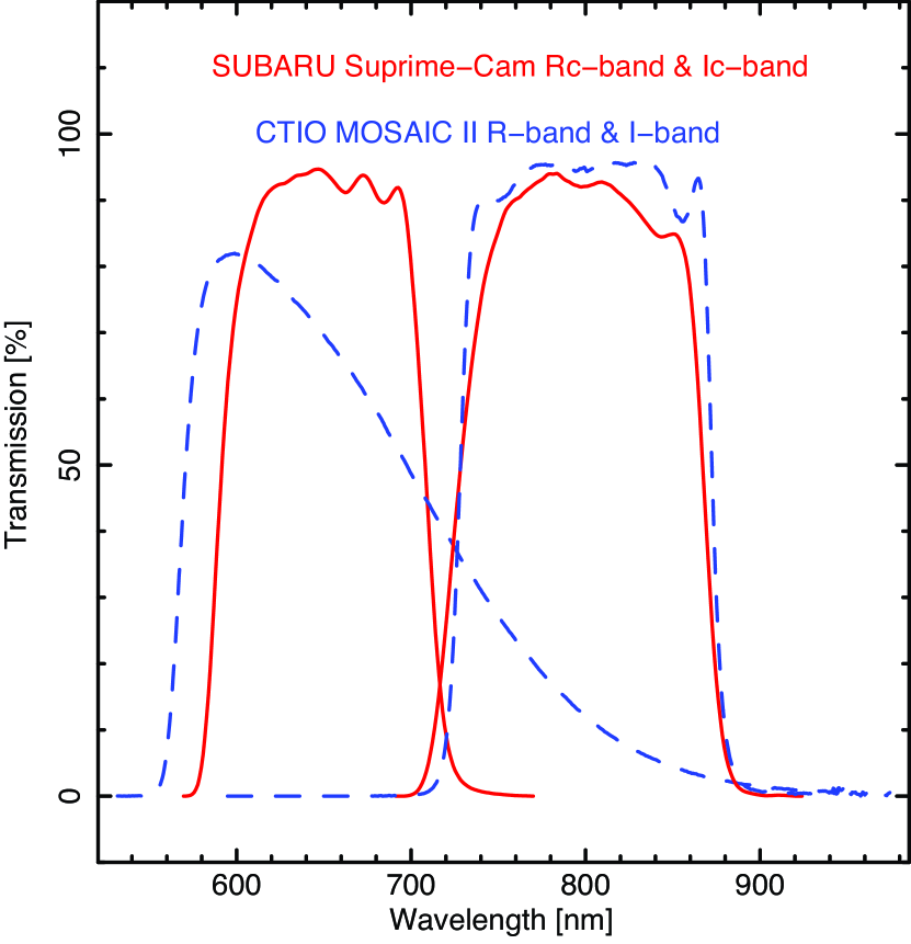
Figure 3.— $R$-band and $I$-band transmission curves for Subaru Suprime-Cam (red solid line) and CTIO MOSAIC II (blue dashed line). The data were obtained from their respective instrumental Web-pages.

3.3. Pan-STARRS1 $z$-band image

Pan-STARRS1 (PS1) $z^{\prime}$-band images were also obtained to determine the host galaxy contamination on the Subaru $z$-band images taken in 2002 September 4. The PS1 telescope has a 1.8-m diameter primary mirror, and it is located at the summit of Mt. Haleakala on Maui. The site and optics deliver a point-spread function (PSF) with a full-width at half-maximum of about 1 arcsec, over a seven square degree field of view. The PS1 was used to conduct a $3\pi$ survey of the entire sky north of $-30^{\circ}$ in $g^{\prime}$-, $r^{\prime}$-, $i^{\prime}$-, $z^{\prime}$- and $y$-band (Magnier et al., 2013; Schlafly et al., 2012; Tonry et al., 2012). Because of the PS1 3$\pi$ surveys strategy, the XRF020903 field was covered during the 3.5 years of survey starting from 2010. The images were processed by the Image Processing Pipeline (Magnier, 2006), and a deeper stacked $z$-band image was generated by the SWarp software (Bertin et al., 2002). The PS1 3$\pi$ catalogs were also used to perform photometric calibration for the $z$-band images taken by Subaru.

3.4. Late phase optical observations

Late optical afterglow in the $R$-band was also monitored by the 1.82 m Copernicus telescope at Mount Ekar (Asiago, Italy) on 2002 September 29 (26.5 days), and by the 3.5m Telescopio Nazionale Galileo (TNG) at La Palma with $V$-, $R$-, and $I$-band filters on 2002 October 2 (29.5 days). Additional $BVRI$ images were obtained with the Danish 1.5-m telescope at the La Silla Observatory between 2002 October 10 (36.8 days) and 14 (40.7 days) and then on October 26 (52.6 days). Differential images without host galaxy contamination were produced from late time images taken in 2004 through image convolution and by using subtraction methods of Alard & Lupton (1998). These photometric results for the optical afterglow against with the secondary standard stars from the list of Henden (2002) were reported by Bersier et al. (2006).

3.5. Radio observations

Very Large Array (VLA) observations were performed at 8.5 GHz on 2002 September 27.22 UT and radio afterglow was detected. Further monitoring observations were made with the VLA over 370 days at frequencies of 1.5, 4.9, 8.5, and 22.5 GHz (Soderberg et al., 2004). The Very Long Baseline Array also observed the radio afterglow and determined the position accurately, as $\alpha_{2000}=22^{\rm h}48^{\rm m}42^{\rm s}.33912\pm 0^{\rm s}.00003$, $\delta_{2000}=-20^{\circ}46^{\prime}08".945\pm 0".0005$ (Soderberg et al., 2004).

4. Data Analysis and Results

4.1. Reduction

The basic reduction of the Suprime-Cam data was performed using the SDFRED package (Ouchi et al., 2004). This entailed bias subtraction and flat-fielding in the $Rc$-, $Ic$- and $z^{\prime}$-band by using a sky flat constructed from the median of the dithered science frames. After performing distortion correction for each object frame, we stacked the frames for each epoch and for each band path filter by considering the median. We performed astrometric calibration for the stacked images against the 3$\pi$ catalog of PS1.

For other data, we used the reduced data as previously summarized, except photometric calibration. The absolute photometric calibration for $Rc$ and $Ic$ was performed using standard stars from the list of Henden (2002). For the photometric calibration of $z$-band images, we used the PS1 $3\pi$ catalog and selected unsaturated stars around the afterglow location.

Table 1Log of Subaru follow-up observations.

Delay (Days)	Filter	Flux density ($\mu$Jy)
0.1645	$Rc$	$21.22\pm 1.09$
0.8609	$Rc$	$34.87\pm 1.38$
1.0087	$Rc$	$35.00\pm 1.39$
1.1378	$Rc$	$29.57\pm 1.28$
35.78945	$Rc$	$3.96\pm 0.46$
0.8991	$Ic$	$49.21\pm 1.82$
1.0436	$Ic$	$41.08\pm 1.67$
0.9569	$z$	$55.67\pm 2.06$
1.0955	$z$	$54.10\pm 1.96$

4.2. Afterglow light curves

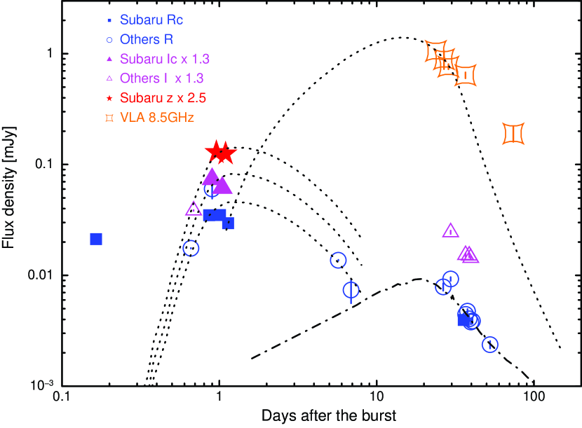
Figure 4.— $Rc/R$, $Ic/I$, $z^{\prime}$-band and VLA 8.5GHz light curves of XRF020903. The dotted lines show the off-axis jet model functions described in §5.1. The dash-dotted line indicates the SN component reported by Bersier et al. (2006).

As Bersier et al. (2006) reported, the host galaxy of XRF020903 is dominated and contaminated in afterglow measurements. Hence, to remove the galaxy contamination, we generated differential images using the HOTPANTS software, which employs an algorithm presented by in Alard & Lupton (1998). We also used special-purpose software based on the same algorithm and tuned to the Subaru/Suprime-Cam data (Urata et al., 2012b) to check the consistency. For $Rc$- and $Ic$-band data of Subaru/Suprime-Cam, we used the $R$- and $I$-band images taken by the CTIO in 2004. The depth of these images was comparable to that of Suprime-Cam images. For the $z$-band, the reference image generated using the PS1 3$\pi$ data was shallower than that of the Subaru image. However, there were the significant signals at the GRB afterglow position in the generated image (Figure 2). Hence, we also generated the differential images by using the same code. As shown in Figure 2, the quality of the differential images is appropriate for estimating the brightness of an afterglow component by the standard aperture photometry. There are appreciable differences between the transmission curves of the Suprime-Cam $Rc$ and CTIO $R$ bands. Figure 3 shows the transmission curves for the Suprime-Cam ($Rc$ and $Ic$) and CTIO ($R$ and $I$) filters. This transmission difference causes a systematic difference of 17% in the magnitudes for an object with a power-law spectrum of index $-1$.

Figure 4 shows the optical light curves for our Subaru data and photometric results reported by Bersier et al. (2006); the radio afterglow light curve at 8.5GHz Soderberg et al. (2004) is also shown. There is a significant signal at 0.165 days after the burst. The use of only one epoch and single-color observations make it difficult to describe the afterglow temporal evolution. When we consider a simple direct connection to the first epoch of $R$ band photometry (0.660 days) made by CTIO, the $Rc/R$ band light curve is flat. The $Rc/R$- and $Ic/I$- band light curves show a clear rapid rebrightening between 0.7 and 0.9 days. The equivalent rising power law index $\alpha$ ($F_{\nu}\propto t^{\alpha}$) are $\sim 2.6$ in the $Rc/R$ and $\sim 2.3$ in the $Ic/I$ band. The multiepochs observations of the Subaru on 2002 September 4 show a flatter and decaying light curve for all three bands. The $Rc/R$ band light curve shows continuous decay up to $\sim$7 days. This indicates that the rebrightening peak was around 0.8$\sim$0.9 days after the burst. As Bersier et al. (2006) demonstrated, there is another late-phase rebrightening peaking at $\sim 20$ days in the $R$ band light curve, which was interpreted as the associated supernova component. The late phase $Rc$-band image taken by Subaru on 2002 October 9 also detected this supernova component in the differential image, and this component is consistent with that observed in the $R$-band within the systematic error.

4.3. Spectral flux distributions

The multiband observations of XRF 020903 were used to determine the spectral flux distribution (SED) at 0.7 and 0.9 day after the burst. To remove the effects of the Galactic interstellar extinction, we used the reddening map of Schlafly & Finkbeiner (2011). Because not all multiband observations were performed exactly at the same epoch, their corresponding fluxes were rescaled to assume a power-law function ($F_{\nu}\propto t^{-\alpha}$). In particular, the brightening phase around 0.7 day was substantially affected. To determine the spectral energy distribution (SED) at 0.7 day, we fixed the time at the epoch of the $B$-band observation (0.695 days). Because the $Rc/R$- and $Ic/I$-band observations were made earlier than $B$ band observations, and the brightening index for $Rc/R$ and $Ic/I$ were estimated as previously described (§4.2). In figure 5, we plot the SED obtained on the basis of the photometric results for $BRI$ bands provided by the CTIO observations. The SED is well fitted by the power-law function as $f(\nu)\propto\nu^{-\beta}$, where $f(\nu)$ is the flux density at frequency $\nu$, and $\beta$ is the spectral index. We have obtained the $\beta$ at 0.695 day as $1.48\pm 0.06$. Similarly, we generated the SED at 0.899 day on basis of the on $Rc$-,$Ic$-, and $z^{\prime}$-band results and obtained a $\beta$ value of $1.43\pm 0.08$, which is consistent with the value for 0.695 day. These results imply that the rebrightening is achromatic.

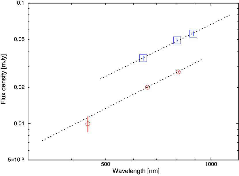
Figure 5.— Spectral flux distribution of the XRF020903 afterglow at 0.695 (red circle point) and 0.899 (blue square points) day. The dashed lines show the best-fit model functions.

5. Discussion

On the basis of the results for XRF020903 described in the preceding section, we discuss the off-axis jet model in the following sections because this model provides a reasonable explanation for this particularly soft XRF. Furthermore this model can explain both the extremely soft prompt emission features and achromatic light curve brightening altogether.

5.1. Off-axis modeling of afterglow light curves

To perform light curves and SEDs modeling for XRF020903, we employed the boxfit code (van Eerten et al., 2012) that involves two-dimensional relativistic hydrodynamical jet simulations for determining the burst explosion parameters, including the off-axis viewing angle and the synchrotron radiation parameters for a homogeneous circumburst medium.

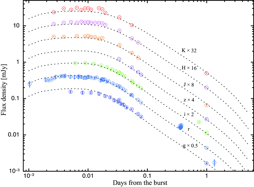
Figure 6.— XRF080330 multi-band light curves with the off-axis jet mode function (dotted lines). The optical and near-infrared data points reported by Guidorzi et al. (2009) were used for the light curve modeling.

In the modeling, we added 17% of the systematic errors to the $R$-band light curve because of the large transmission differences, as shown in Figure 3. To perform light curve modeling, we focused on the data between 0.6 and 8 day because the observed optical light curve showed achromatic brightening between 0.7 and 0.8 day after the burst, which is unusual among the well-observed afterglows. The later phase (from $\sim$20 days) was excluded in the modeling because it is likely to be the SN component Bersier et al. (2006). We also excluded the single data point at 0.16 day because the sparse monitoring and single detection at 0.16 day make it difficult to decode the light curve between 0.16 and 0.7 day. The consideration of different components (one component faded away before 0.6 day and the other was rebrightening) was reasonable because connecting the light curve between 0.16 and 0.7 day smoothly produced a flat evolution, indicating long lasting ($\sim$0.6 days) energy injection. Using multicolor optical data between 0.6 day and 8 days and the radio 8.5 GHz radio data, we performed light curve modeling. We examined the light curves for various values of $\theta_{jet}$ and $\theta_{obs}$. The range of $\theta_{jet}$ covered most of the estimated values for classical GRBs (from 0.04 rad to 0.5 rad), while $\theta_{obs}$ varied from 0.0 rad to 1.5 rad when an at least 3-fold enhancement of $\theta_{jet}$ was examined. Figure 4 shows the best-fit model functions that describe the achromatic rebrightening, $R/Rc$-band temporal evolution, and radio brightness. The derived burst parameters are also presented in Table 2. There are two notable features. The first is the jet opening half angle $\theta_{jet}$ of 0.1 rad, which is consistent with those of classical hard GRBs (see Figure 6 in Fong et al., 2012). The second is the large observing angle ($\theta_{obs}\sim 0.21$ rad), which corresponds to $\theta_{obs}\sim 2\theta_{jet}$.

To compare with other samples such as an off-axis origin XRF candidate, classical hard GRB, XRR, and the on-axis orphan GRB candidates, we considered 080330, 990510, 120326A, 131030A, and PTF11agg (Table 2). The burst parameters for these bursts, except 080330, were also determined by using the same box fit code on the basis of multifrequency afterglow observations (van Eerten et al., 2012; Urata et al., 2014, 2015; Cenko et al., 2013). To compare the burst parameters of XRF080330 with those of XRF020903 and others, we also performed the multiband light curve modeling with the same code by using available multiband photometric results Guidorzi et al. (2009). XRF080330 was detected by Swift and an afterglow in optical and IR bands showed the achromatic brightening phase that could be interpreted using the off-axis jet model (Guidorzi et al., 2009). However, $E^{src}_{peak}$ was not well characterized, as being less than 88 keV (Guidorzi et al., 2009), because of the relatively high and narrow energy band of Swift/BAT. In addition, the large uncertainties in the of fluence ratio of the prompt emission ($1.5^{+0.7}_{-0.3}$) were still compatible with an XRR category based on the modified XRF/XRR definition for Swift/BAT (Sakamoto et al., 2008). As shown in Figure 6, the achromatic brightening light curves were well modeled, and the derived burst parameters are presented in Table 2. One of the key features was $\theta_{obs}$(=0.12 rad), which was equal to $\theta_{jet}$(0.12 rad). Thus, the achromatic brightening is explained by the off-axis jet model. However, our viewing angle ($\theta_{obs}\sim\theta_{jet}$) was not larger as estimated by Guidorzi et al. (2009) ($\theta_{obs}\sim 1.5-2\times\theta_{jet}$).

This enables a comparison of the burst parameters, which are presented in Table 2. We also list the observed features of the prompt emission. The observed values are widely distributed to represent the variety of GRB classes. By contrast, the parameters obtained through the afterglow modeling are comparable to each other, except for $\theta_{obs}$. Thus, the off-axis jet model is suitable for explaining the diverse afterglow light curves and the GRB category.

Table 2Summary of burst parameters obtained by observations and numerical modeling

Parameters	020903	080330	990510	131030A	120326A	PTF11agg
Category	XRF	XRF(XRR?)	GRB	GRB	XRR	on-axis orphan(?)
$E^{src}_{peak}$ (keV)	3.3${}^{+1.8}_{-1.0}$	$<88$	423${}^{+42}_{-42}$	$406\pm 22$	107.8${}^{+15.3}_{-15.3}$	$-$
$E_{iso}$ (erg)	1.4${}^{+18.0}_{-0.7}\times 10^{49}$	$<2.2\times 10^{52}$	2.1${}^{+0.3}_{-0.3}\times 10^{53}$	$3.0^{+2.0}_{-0.2}\times 10^{53}$	3.2${}^{+0.4}_{-0.3}\times 10^{52}$	$-$
$z$	0.251	1.51	1.619	1.293	1.798	0.5$<z<$3.0
$\theta_{jet}$ (rad)	0.10	0.12	0.075	0.15	0.14	0.20
$E$ (erg)	$5.9\times 10^{52}$	$2.3\times 10^{52}$	$1.8\times 10^{53}$	$3.4\times 10^{52}$	$3.9\times 10^{52}$	$9\times 10^{52}$
$n$ (cm-3)	1.1	9.0	0.03	0.3	1.0	0.001
$\theta_{obs}$ (rad)	0.21	0.12	0 (fixed)	0 (fixed)	0 (fixed)	0.19
$p$	2.8	2.1	2.28	2.1	2.5 (fixed)	3.0
$\epsilon_{B}$	$1.4\times 10^{-3}$	$1.6\times 10^{-1}$	$4.6\times 10^{-3}$	$4.4\times 10^{-2}$	$1.0\times 10^{-3}$	$4\times 10^{-2}$
$\epsilon_{e}$	$2.9\times 10^{-1}$	$1.4\times 10^{-1}$	$3.7\times 10^{-1}$	$2.7\times 10^{-1}$	$6.9\times 10^{-1}$	$2\times 10^{-1}$
$\chi^{2}/dof$	90.9/9 (10.1)	512.5/125 (4.1)	1267.2/198 (6.4)	$-$	28.0/20 (1.4)	$-$
Data	Opt, Radio	Opt	X,Opt,Radio	Opt, ALMA	Opt	Opt, Radio
Ref.	This work	This work	van Eerten et al. (2012)	Urata et al. (2015)	Urata et al. (2014)	Cenko et al. (2013)

5.2. Small values of $E^{src}_{peak}$ and $E_{iso}$ with the Off-axis model

Using the values of $\theta_{jet}$ and $\theta_{obs}$ obtained by fitting afterglow light curves (Table 2), we discuss on observed small values of $E^{src}_{peak}$ and $E_{iso}$ to verify the off-axis jet model. We adopted a simple model with a top-hat profile of the prompt emission of relativistic jet (Granot et al., 1999; Woods & Loeb, 1999; Ioka & Nakamura, 2001; Yamazaki et al., 2002). Following the formalism derived by Graziani et al. (2006) and Donaghy (2006), the peak energy $E^{src}_{peak}(\theta_{obs})$ and the isotropic energy $E_{iso}(\theta_{obs})$ were analytically derived as functions of $\theta_{obs}$, $\theta_{jet}$, and the Lorentz factor of the jet $\gamma=(1-\beta^{2})^{-1/2}$. We defined the ratios $R_{1}$ and $R_{2}$ as

$$R_{1} = \frac{E^{src}_{peak}(\theta_{obs})}{E^{src}_{peak}(0)}$$ (1)

$$= \frac{2(1-\beta)(1-\beta\cos\theta_{jet})}{2-\beta(1+\cos\theta_{jet})}$$

$$\times\frac{f(\beta-\cos\theta_{obs})-f(\beta\cos\theta_{jet}-\cos\theta_{obs})}{g(\beta-\cos\theta_{obs})-g(\beta\cos\theta_{jet}-\cos\theta_{obs})}~{}~{},$$

$$R_{2} = \frac{E_{iso}(\theta_{obs})}{E_{iso}(0)}$$

$$= \frac{(1-\beta)^{2}(1-\beta\cos\theta_{jet})^{2}}{\beta(1-\cos\theta_{jet})[2-\beta(1+\cos\theta_{jet})]}$$

$$\times\left[f\left(\beta-\cos\theta_{obs}\right)-f\left(\beta\cos\theta_{jet}-\theta_{obs}\right)\right]~{}~{},$$

where

$$f(z)=$$

$$\frac{\gamma^{2}(2\gamma^{2}-1)z^{3}+(3\gamma^{2}\sin^{2}\theta_{obs}-1)z+2\cos\theta_{obs}\sin^{2}\theta_{obs}}{|z^{2}+\gamma^{-2}\sin^{2}\theta_{obs}|^{\frac{3}{2}}}~{}~{},$$ (3)

$$g(z)=\frac{2\gamma^{2}z+2\cos\theta_{obs}}{|z^{2}+\gamma^{-2}\sin^{2}\theta_{obs}|^{\frac{1}{2}}}~{}~{}.$$ (4)

For fixed $\theta_{jet}$ and $\gamma$, it can be seen that for $\theta_{obs}>\theta_{jet}$ (see Figure 2 of Donaghy, 2006), both $E^{src}_{peak}$ and $E_{iso}$ decreases with an increase in $\theta_{obs}$ because of the relativistic beaming effect.

We consider the case of XRF 020903. In the following, we fix $\theta_{obs}=0.21$ rad and $\theta_{jet}=0.1$ rad. Subsequently, ratios $R_{1}$ and $R_{2}$ are calculated for given $\gamma$. For example, we find $R_{1}=3.45\times 10^{-3}$ and $R_{2}=1.23\times 10^{-6}$ if $\gamma=100$. Classical hard GRBs typically have $E^{src}_{peak}=500$ keV (Nava et al., 2012), and therefore we first assume $E^{src}_{peak}(0)=500$ keV. We then find that $E^{src}_{peak}(\theta_{obs}=0.21)=4.2$ keV, which is close to the observed result for XRF 020903. Furthermore, for the observed value of $E_{iso}$, we consider $E_{iso}(\theta_{obs}=0.21)=1.4\times 10^{49}$erg, resulting in $E_{iso}(0)=1.9\times 10^{54}$erg. In summary, if a jet with $\theta_{jet}=0.1$ and $\gamma=100$ is seen on-axis ($\theta_{obs}=0$), we would have $E^{src}_{peak}=500$ keV and $E_{iso}=1.9\times 10^{54}$erg, which is almost consistent with the ${E^{\rm src}_{\rm peak}-E_{\rm iso}}$ relation (Amati et al., 2002; Nava et al., 2012). The empirical relation could be an indicator of GRB category although the background physics are not yet fully understood. In fact, classical hard GRBs show the relation, but short GRBs do not exhibit it. Hence, the observed small values of $E^{src}_{peak}$ and $E_{iso}$ for XRF 020903 are naturally explained by the off-axis jet model.

We also discuss parameter dependence. In the following, we fix $\theta_{obs}=0.21$ rad, $\theta_{jet}=0.1$ rad, and $E_{iso}(\theta_{obs})=1.4\times 10^{49}$erg. The observed best fit value $E^{src}_{peak}(\theta_{obs}=0.21)=3.3$ keV is reproduced for $\gamma=112$ and $E^{src}_{peak}(0)=500$ keV, and we obtain $E_{iso}(0)=3.0\times 10^{54}$erg. For $E^{src}_{peak}(0)=250$ keV, we need a smaller $\gamma$ value (79) is required to obtain $E^{src}_{peak}(\theta_{obs}=0.21)=3.3$ keV, and we find $E_{iso}(0)=7.6\times 10^{53}$erg. Similarly, when we consider $E^{src}_{peak}(0)=1$ MeV, we have $\gamma=160$ and $E_{iso}(0)=1.3\times 10^{55}$erg. For these cases, the on-axis values, $E^{src}_{peak}(0)$ and $E_{iso}(0)$ remain within the 3$\sigma$ scatter of the ${E^{\rm src}_{\rm peak}-E_{\rm iso}}$ relation. These values of $\gamma$ are consistent with those measured using the onset of optical afterglows. Liang et al. (2010) reported $\gamma$ measurements that were distributed from $\sim 90$ to $\sim 600$ as well as a significant proportion of events that exhibited values below 200. However, the values are lower than the prediction ($\gamma>300$ for all GRBs) made by Donaghy (2006) for reducing the number of unseen events away from the observed ${E^{\rm src}_{\rm peak}-E_{\rm iso}}$ and ${E^{src}_{peak}-E_{\gamma}}$ (Ghirlanda et al., 2004) relations. Here, $\rm E_{\gamma}$ is the jet collimation-corrected energy. The simplest off-axis jet models for XRFs (Yamazaki et al., 2002, 2003) adopt low values of $\gamma$ ($\sim 100$) and predict a large number of events away from these relations that are not observed (see Figures 4-9 in Donaghy (2006)). Therefore something more complicated procedures must be required. For one of examples, Donaghy (2006) described that a inverse correlation between $\gamma$ and the opening solid angle of the GRB jet has the effect of greatly reducing the visibility of off-axis events.Another possibility is to consider more complicated jet structure (e.g. Salafia et al., 2015).

The spectral peak energy of XRF020903 is conservatively determined only the upper limit, reported by Sakamoto et al. (2004). Although XRF020903 also followed the $E^{src}_{peak}-E_{iso}$ relation when we employed the value estimated by the constrained Band function with the 90% confident level, four of the five HETE-2 XRFs (including XRF 020903) with the lowest upper limits on $E^{obs}_{peak}$ were potential outlier events of the $E^{src}_{peak}-E_{iso}$ and the $L_{iso}-E^{src}_{peak}$ relations. Because these events are outliers in the $E^{obs}_{peak}-F^{p}_{N}$ (Figure 1 in Sakamoto et al. (2005) and Figure 9 in Lamb et al. (2005)) and the $E^{obs}_{peak}-S_{E}$ planes (Figure 2 in Donaghy, 2006). Here, $F^{p}_{N}$ and $S_{E}$ denote the peak photon number flux of the burst and the energy fluence, respectively. These results indicate that the nature of these four XRFs $-$ and therefore the nature of XRFs in general $-$ might differ considerably from those of the rest of the XRFs, XRRs, and GRBs. However, our result on one of the four outlier events contradicts this suggestion. Hence, we may be able to explain the remaining three lowest $E^{obs}_{peak}$ events in an identical manner, although additional adjustments on the jet geometry or the initial Lorentz factor could be required.

5.3. Prospect with optical surveys

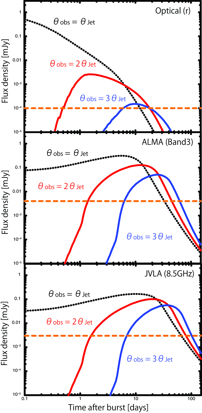
Figure 7.— Expected off-axis GRB afterglow light curves with observing angle of $2\theta_{jet}$ (red solid line) and $3\theta_{jet}$ (blue solid line) at $z=1$ in the $r^{\prime}$-band (top), ALMA Band3 (middle), and JVLA 8.5 GHz (bottom) obtained from the off-axis jet modeling of XRF020903. The dash orange lines indicate the sensitivity limit of Subaru ($r^{\prime}$-band), ALMA (Band3), or JVLA (8.5GHz) with 1 h exposure.

Finding off-axis orphan afterglows through untargeted optical surveys is also a crucial method for establishing a unified picture of GRBs. Several optical time-domain surveys performed using telescopes with diameters in the range of 1-2m (e.g. iPTF, Pan-STARRS1) have reported intriguing new discoveries related to stellar explosions. However, the sensitivities of these surveys were insufficient for detecting faint off-axis orphan afterglows. Hence, off-axis orphan GRB afterglows are yet to be observationally confirmed. However, a new wide-field-of-view camera $--$Hyper-Suprime-Cam (HSC)$--$ attached to the Subaru telescope and the planned LSST have considerable capabilities to detect the first off-axis orphan GRB afterglow in untargeted time-domain surveys.

One of the challenges in generic transient surveys is determining candidates from the various types of optical transients, because the occurrence of GRB orphan afterglows is rarer compared with that of known types of supernova. These candidate selection can be performed using optical photometric survey data and a proper photometric transient classification. The photometric classification involves seven steps: (1) finding transient candidates by generating differential images, (2) generating light curves for transient components, (3) identifying host galaxies, (4) determining a transient location in their hosts, (5) matching the candidates with known sources in various catalogs, (6) matching light curves and color evolution, and (7) estimating the photometric redshift of hosts. For Step (1) and (2), we can employ the algorithm (Alard & Lupton, 1998) as described in §4 and Urata et al. (2012b). For Step (3), (4), and (7), a considerable number of GRB host galaxy observations have been performed in the optical and near-infrared range. Systematic unbiased observations have also been performed using VLT (Hjorth et al., 2012). The brightness range of host galaxies for GRBs for $z<2$ is 23.0$--$26.5 mag (e.g., Berger, 2010). Since the redshift range of a considerable number of orphan GRB afterglows with HSC surveys extends up to $z\sim 2$, HSC images (e.g. reference images for PSF matched subtraction) are sufficiently deep to detect these host galaxies. Thus, we can also perform the photometric redshift for the host galaxies. Photometric redshift for GRB host galaxies is also effective (e.g., Christensen et al., 2004). Hence, the light curve expectations basis of off-axis jet origin of XRFs are crucial to establish a effective candidate searches.

Figure 7 shows the expected off-axis afterglow light curves at $z=1$ along with various observing angles ($\theta_{obs}=\theta_{jet}$, $2\theta_{jet}$, and $3\theta_{jet}$) in the optical $r$-band, ALMA Band3, and JVLA 8.5 GHz, obtained from the light curve modeling of XRF020903. The orange dashed lines in Figure 7 indicate the sensitivity limit for 1 h exposure for each instrument. Hence, off-axis orphan GRB afterglows (up to $\sim 3\theta_{jet}$) can be detected in optical time-domain surveys by using 8m class telescopes. Follow-up radio observations are also crucial for confirmation of orphan afterglows and identification of constraints on their physical parameters, as shown in Figure 7. Because radio temporal evolution is substantially slower than that of optical temporal evolution, long-term monitoring by using ALMA and/or JVLA with reasonable exposure ($\sim$1h) requires the confirmation of the optical candidates.

6. Conclusion

We studied XRFs on the basis of redshift measurements, multifrequency afterglow modeling, and spectral peak measurements ($E^{src}_{peak}$) to verify the off-axis jet model and to provide feedback to ongoing and planned optical time-domain surveys, which have considerable potential for detecting off-axis orphan GRB afterglows. Because off-axis orphan GRB afterglows are produced as a natural consequence of GRB jets production, the confirmation of the off-axis origin of XRFs is the necessary to conduct off-axis orphan GRB afterglow surveys.

To verify the off-axis jet model, we selected XRF020903 by considering the three aforementioned sample selection factors. For this event, we reduced the archived data of Subaru to describe the optical light curves, and found achromatic rebrightening at $\sim$0.7 days. Using these optical results and radio data obtained from literature, we performed afterglow light curve modeling with the boxfit code and found that the off-axis jet model ($\theta_{obs}\sim 2\theta_{jet}$) could explain the achromatic rebrightening, $R/Rc$-band temporal evolution, and radio brightness.

We also compared the burst parameters of XRF020903 with those of other categories of events, such as a classical hard GRB, an XRR, and an on-axis orphan GRB candidate. For XRF080330, we performed light curve modeling in a manner similar to that used for XRF020903 by using optical data from literature, and we confirmed that the off-axis jet model ($\theta_{obs}\sim\theta_{jet}$) could describe the optical afterglow light curves. We also listed the observed features of the prompt emission for each event. The observed values were too widely distributed to represent the classical hard GRB, XRR, and XRF. By contrast, the parameters obtained from the afterglow modeling were comparable to each other, except for $\theta_{obs}$. Thus, the off-axis jet model was found to be suitable for explaining the diverse afterglow light curves and the GRB category.

We also verified the observed small values of $E^{src}_{peak}$ and $E_{iso}$ by adopting a simple model with a top-hat profile of the prompt emission of a relativistic jet. The parameters $E^{src}_{peak}(\theta_{obs})$ and $E_{iso}(\theta_{obs})$ were analytically derived as functions of $\theta_{obs}$, $\theta_{jet}$, and $\gamma=(1-\beta^{2})^{-1/2}$. By fixing $\theta_{obs}$ and $\theta_{jet}$ as 0.21 and 0.1 rad, respectively, we evaluated $\gamma$, $E^{src}_{peak}$, and $E_{iso}$ observed from the on-axis of the jet ($E^{src}_{peak}(0)$ and $E_{iso}(0)$). These expected values were consistent with those of classical hard GRBs, and the observed small values of $E^{src}_{peak}$ and $E_{iso}$ of XRF 020903 could be naturally explained by the off-axis jet model.

Finally, we expected off-axis orphan GRB afterglow light curves at $z=1$ along with three viewing angles on the basis of the XRF afterglow light curve modeling. To detect these light curves, especially afterglows with a larger viewing angle ($\theta_{obs}>2\theta_{jet}$), an 8-m class telescope with wide-field imagers, such as the LSST and Subaru/HSC, is required. Off-axis orphan GRB afterglows up to $\sim 3\theta_{jet}$ can be discovered by performing time-domain surveys with an 8-m class telescope. Because such optical time-domain surveys also detect numerous other optical transients, we presented expected radio afterglow light curves for the confirmation and determination of burst parameters. Radio light curves can be monitored using ALMA and JVLA with reasonable exposure.

References

- Alard & Lupton (1998) Alard & Lupton 1998, ApJ, 503, 325
- Amati et al. (2002) Amati, L., 2002, A&A, 390, 81
- Baba, H et al. (2002) Baba, H., et al., 2002, ASP Conference Series, Vol. 281, 298
- Band et al. (1993) Band, D., 1993, ApJ, 413, 281
- Barthelmy et al. (2005) Barthelmy, S. D., Barbier, L. M., Cummings, J. R., et al. 2005, Space Sci. Rev., 120, 143
- Berger (2010) Berger, E. 2010, ApJ, 722, 1946
- Bersier et al. (2006) Bersier, D., Fruchter, A. S., Strolger, L.-G., et al. 2006, ApJ, 643, 284
- Bertin et al. (2002) Bertin, E., Mellier, Y., Radovich, M., et al. 2002, Astronomical Data Analysis Software and Systems XI, 281, 228
- Cenko et al. (2013) Cenko, S. B., Kulkarni, S. R., Horesh, A., et al. 2013, ApJ, 769, 130
- Christensen et al. (2004) Christensen, L., Hjorth, J., & Gorosabel, J. 2004, A&A, 425, 913
- Donaghy (2006) Donaghy, T. Q. 2006, ApJ, 645, 436
- Fong et al. (2012) Fong, W., Berger, E., Margutti, R., et al. 2012, ApJ, 756, 189
- Ghirlanda et al. (2004) Ghirlanda, G., Ghisellini, G., & Lazzati, D. 2004a, ApJ, 616, 331
- Granot et al. (1999) Granot, J., Piran, T., & Sari, R. 1999, ApJ, 513, 679
- Graziani et al. (2006) Graziani, C., Lamb, D. Q., & Donaghy, T. 2006, Gamma-Ray Bursts in the Swift Era, 836, 117 (astro-ph/0505623)
- Guidorzi et al. (2009) Guidorzi, C., Clemens, C., Kobayashi, S., et al. 2009, A&A, 499, 439
- Heise et al. (2001) Heise, J., Zand, J. I., Kippen, R. M., & Woods, P. M. 2001, Gamma-ray Bursts in the Afterglow Era, 16
- Heise (2003) Heise, J. 2003, Gamma-Ray Burst and Afterglow Astronomy 2001: A Workshop Celebrating the First Year of the HETE Mission, 662, 229
- Henden (2002) Henden, A. 2002, GRB Coordinates Network, 1571, 1
- Hjorth et al. (2012) Hjorth, J., Malesani, D., Jakobsson, P., et al. 2012, ApJ, 756, 187
- Huang et al. (2002) Huang, Y. F., Dai, Z. G., & Lu, T. 2002, MNRAS, 332, 735
- Ioka & Nakamura (2001) Ioka, K., & Nakamura, T. 2001, ApJ, 554, L163
- Jager et al. (1997) Jager, R., Mels, W. A., Brinkman, A. C., et al. 1997, A&AS, 125, 557
- Kaneko et al. (2006) Kaneko, Y., Preece, R. D., Briggs, M. S., et al. 2006, ApJS, 166, 298
- Kippen et al. (2001) Kippen, R. M., Woods, P. M., Heise, J., et al. 2001, Gamma-ray Bursts in the Afterglow Era, 22
- Lamb et al. (2005) Lamb, D. Q., Donaghy, T. Q., & Graziani, C. 2005, ApJ, 620, 355
- Liang et al. (2010) Liang, E.-W., Yi, S.-X., Zhang, J., et al. 2010, ApJ, 725, 2209
- Lien et al. (2015) Lien, A., et al. ApJS in prep.
- Magnier et al. (2013) Magnier, E. A., Schlafly, E., Finkbeiner, D., et al. 2013, ApJS, 205, 20
- Magnier (2006) Magnier, E. 2006, The Advanced Maui Optical and Space Surveillance Technologies Conference,
- Malesani et al. (2008) Malesani, D., Fynbo, J. P. U., Jakobsson, P., Vreeswijk, P. M., & Niemi, S.-M. 2008, GRB Coordinates Network, 7544, 1
- Matsuoka et al. (2009) Matsuoka, M., Kawasaki, K., Ueno, S., et al. 2009, PASJ, 61, 999
- Miyazaki et al. (2002) Miyazaki, S., et al. 2002, PASJ, 54, 833
- Miyazaki et al. (2012) Miyazaki, S., Komiyama, Y., Nakaya, H., et al. 2012, Proc. SPIE, 8446, 84460Z
- Nava et al. (2012) Nava, L. et al. 2012, MNRAS, 421, 1256
- Ohno et al. (2008) Ohno, M., Fukazawa, Y., Takahashi, T., et al. 2008, PASJ, 60, 361
- Ouchi et al. (2004) Ouchi, M., Shimasaku, K., Okamura, S., et al. 2004, ApJ, 611, 660
- Pierfederici et al. (2004) Pierfederici, F., Valdes, F., Smith, C., Hiriart, R., & Miller, M. 2004, Astronomical Data Analysis Software and Systems (ADASS) XIII, 314, 476
- Pierfederici (2006) Pierfederici, F. 2006, Astronomical Data Analysis Software and Systems XV, 351, 433
- Rhoads (1999) Rhoads, J. E., 1999, ApJ, 525, 737
- Sakamoto et al. (2004) Sakamoto, T., Lamb, D. Q., Graziani, C., et al. 2004, ApJ, 602, 875
- Sakamoto et al. (2005) Sakamoto, T., Lamb, D. Q., Kawai, N., et al. 2005, ApJ, 629, 311
- Sakamoto et al. (2008) Sakamoto, T., Hullinger, D., Sato, G., et al. 2008, ApJ, 679, 570
- Salafia et al. (2015) Salafia, O. S., Ghisellini, G., Pescalli, A., Ghirlanda, G., & Nappo, F. 2015, arXiv:1502.06608
- Sari et al. (1999) Sari, R., Piran, T., & Halpern, J. P. 1999, ApJ, 519, L17
- Schlafly et al. (2012) Schlafly, E. F., Finkbeiner, D. P., Jurić, M., et al. 2012, ApJ, 756, 158
- Schlafly & Finkbeiner (2011) Schlafly, E. F., & Finkbeiner, D. P. 2011, ApJ, 737, 103
- Serino et al. (2014) Serino, M., Sakamoto, T., Kawai, N., et al. 2014, PASJ, 66, 87
- Shirasaki et al. (2003) Shirasaki, Y., Kawai, N., Yoshida, A., et al. 2003, PASJ, 55, 1033
- Soderberg et al. (2004) Soderberg, A. M., Kulkarni, S. R., Berger, E., et al. 2004, ApJ, 606, 994
- Tonry et al. (2012) Tonry, J. L., Stubbs, C. W., Lykke, K. R., et al. 2012, ApJ, 750, 99
- Urata et al. (2012a) Urata, Y., Huang, K., Yamaoka, K., Tsai, P. P., & Tashiro, M. S. 2012, ApJ, 748, L4
- Urata et al. (2012b) Urata, Y., Tsai, P. P., Huang, K., et al. 2012, ApJ, 760, LL11
- Urata et al. (2014) Urata, Y., Huang, K., Takahashi, S., et al. 2014, ApJ, 789, 146
- Urata et al. (2015) Urata, Y., Huang, K, et al. 2015, ApJ, in prep.
- van Eerten et al. (2012) van Eerten, H., van der Horst, A., & MacFadyen, A. 2012, ApJ, 749, 44
- von Kienlin et al. (2014) von Kienlin, A., Meegan, C. A., Paciesas, W. S., et al. 2014, ApJS, 211, 13
- Woods & Loeb (1999) Woods, E., & Loeb, A. 1999, ApJ, 523, 187
- Yamaoka et al. (2009) Yamaoka, K.., et al. 2009, PASJ, 61, S35
- Yamazaki et al. (2002) Yamazaki, R., Ioka, K., & Nakamura, T. 2002, ApJ, 571, L31
- Yamazaki et al. (2003) Yamazaki, R., Ioka, K., and Nakamura, T., 2003, ApJ, 593, 941
- Zhang et al. (2004) Zhang, B., Dai, X., Lloyd-Ronning, N. M., & Mészáros, P. 2004, ApJ, 601, L119