Conductance and absolutely continuous spectrum of 1D samples

Abstract. We characterize the absolutely continuous spectrum of the one-dimensional Schrödinger operators $h=-\Delta+v$ acting on $\ell^{2}({\mathbb{Z}}_{+})$ in terms of the limiting behaviour of the Landauer-Büttiker and Thouless conductances of the associated finite samples. The finite sample is defined by restricting $h$ to a finite interval $[1,L]\cap{\mathbb{Z}}_{+}$ and the conductance refers to the charge current across the sample in the open quantum system obtained by attaching independent electronic reservoirs to the sample ends. Our main result is that the conductances associated to an energy interval $I$ are non-vanishing in the limit $L\to\infty$ iff ${\rm sp}_{\rm ac}(h)\cap I\neq\emptyset$. We also discuss the relationship between this result and the Schrödinger Conjecture [Av, BJP].

1 Introduction

This paper concerns a connection between two directions of research: transport theory of open quantum systems and spectral theory of discrete Schrödinger operators. The simplest open quantum system where this connection is exhibited, the so-called electronic black box model (EBBM), consists of a finite sample connecting two free electron reservoirs. The model is considered in the independent electron and tight binding approximations and the object of study is the charge current across the sample induced by the voltage differential between the reservoirs. The celebrated Landauer-Büttiker and Thouless current/conductance formulas of finite samples arose from such considerations.

In this work we shall restrict ourselves to 1D geometry. The one-particle configuration space of a sample of length $L$ is the finite set ${\mathbb{Z}}_{L}=\{1,2,\ldots,L\}$. Left and right electronic reservoirs are attached to the sample at site $1$ and $L$, respectively (see Figure 1). We denote by ${\mathbb{Z}}_{+}$ the positive integers. To a potential $v:{\mathbb{Z}}_{+}\rightarrow{\mathbb{R}}$ we associate the discrete Schrödinger operator

$$h=-\Delta+v,$$

acting on the Hilbert space $\ell^{2}({\mathbb{Z}}_{+})$. We shall view ${\mathbb{Z}}_{+}$ as the one-particle configuration space and $h$ as the Hamiltonian of the extended sample. The one-particle Hamiltonian of the sample of length $L$ is obtained by restricting $h$ to $\ell^{2}({\mathbb{Z}}_{L})$. We are interested in the relationship between the spectral properties of the extended Hamiltonian $h$ and the limiting values of the Landauer-Büttiker and Thouless current/conductance of the finite sample as $L\rightarrow\infty$. More specifically, we will focus on the relationship between:

1. The physical characterization of the conducting regime of the extended sample as the set of energies at which the current/conductance is non-vanishing in the limit $L\rightarrow\infty$.

2. The mathematical characterization of the conducting regime of the extended sample as the absolutely continuous spectrum of $h$, denoted ${\rm sp}_{\rm ac}(h)$.

The recent rigorous proofs of the Landauer-Büttiker and Thouless current/conductance formulas from the first principles of quantum statistical mechanics [AJPP, N, BJLP1, BSP] have opened the way to the study of the equivalence ${\rm(A)}\Leftrightarrow{\rm(B)}$. Some preliminaries are required to formulate this equivalence in mathematically precise terms.

Figure 1: A finite sample of length $L$ coupled to two electronic reservoirs

We shall assume that the left and right reservoirs are in thermal equilibrium at zero temperature and chemical potentials $\mu_{l}<\mu_{r}$. The role of the chemical potentials is to "probe" the sample in the energy interval $[\mu_{l},\mu_{r}]$. In the large time limit, the potential differential $\mu_{r}-\mu_{l}$ induces a steady charge current across the sample. The expectation value ${\cal J}_{\rm LB}(L,\mu_{l},\mu_{r})$ of this steady current is given by the Landauer-Büttiker formula (2.2)-(2.3). This formula depends intrinsically on the structure of the reservoirs and on the form of their coupling to the sample. One particular choice of the reservoirs/couplings leads to the Thouless current formula which we denote by ${\cal J}_{\rm Th}(L,\mu_{l},\mu_{r})$, see Section 2.2. The respective conductances are

$$G_{{\rm LB}}(L,\mu_{l},\mu_{r})=\frac{1}{\mu_{r}-\mu_{l}}{\cal J}_{{\rm LB}}(L,\mu_{l},\mu_{r})\quad{\rm and}\quad G_{{\rm Th}}(L,\mu_{l},\mu_{r})=\frac{1}{\mu_{r}-\mu_{l}}{\cal J}_{{\rm Th}}(L,\mu_{l},\mu_{r}).$$

In our analysis, current and conductance play similar roles, and in the sequel we will switch between these two notions depending on notational convenience. We shall review the Landauer-Büttiker and Thouless formulas in Section 2. To avoid trivialities when using the Landauer-Büttiker formula we shall assume that the reservoirs are transparent for the energies in the interval $(\mu_{l},\mu_{r})$ (see Definition 2.1 below).

A mathematically precise formulation of the equivalence ${\rm(A)}\Leftrightarrow{\rm(B)}$ is the object of the following two conjectures, which should hold for any potential $v$:

Conjecture I. If $(\mu_{l},\mu_{r})\cap{\rm sp}_{\rm ac}(h)=\emptyset$, then

$$\lim_{L\rightarrow\infty}G_{\#}(L,\mu_{l},\mu_{r})=0,$$

where $\#$ stands for LB or Th.

Conjecture II. If $(\mu_{l},\mu_{r})\cap{\rm sp}_{\rm ac}(h)\not=\emptyset$, then

$$\liminf_{L\rightarrow\infty}G_{\#}(L,\mu_{l},\mu_{r})>0,$$

where $\#$ stands for LB or Th.

Just like the celebrated Schrödinger Conjecture [MMG, Si2, Av], which we will discuss below, Conjectures I and II are rooted in the formal computations and implicit assumptions of the physicists working on the subject. To the best of our knowledge, they were first formulated in the above mathematical form in [Las1] which treats the case $\#={\rm Th}$ in the setting of ergodic Schrödinger operators. We refer the reader to [Las1] for references regarding early physicists’ work that motivated the conjectures and to [CGM] for supporting numerical results. Conjectures I and II are also of importance for the foundations of quantum mechanics since they would provide the first complete dynamical characterization of the absolutely continuous spectrum of Schrödinger operators.

A strong form of Conjectures I and II in the case $\#={\rm LB}$ was studied in the recent work [BJP]. There, the focus was on the Landauer-Büttiker spectral density defined by

$${\cal D}_{\rm LB}(L,E)=\lim_{\delta\downarrow 0}G_{\rm LB}(L,E-\delta,E+\delta).$$ (1.1)

The limit (1.1) exists for Lebesgue a.e. $E\in{\mathbb{R}}$, takes values in $[0,(2\pi)^{-1}]$, and is such that

$${\cal J}_{{\rm LB}}(L,\mu_{l},\mu_{r})=\int_{\mu_{l}}^{\mu_{r}}{\cal D}_{\rm LB}(L,E){\rm d}E.$$ (1.2)

Although the density ${\cal D}_{\rm LB}(L,E)$ depends intrinsically on the structure of the reservoirs and the choice of the coupling, it does not depend on the choice of the thermodynamical states of the reservoirs, and in particular it does not depend on the choice of $\mu_{l/r}$. For more information about ${\cal D}_{\rm LB}(L,E)$, we refer the reader to Section 2.1.

In our setting, the transfer matrices of $h$ provide the link between transport and spectrum. We denote by

$$T(L,E)=\left[\begin{matrix}v(L)-E&-1\\ 1&0\end{matrix}\right]\cdots\left[\begin{matrix}v(1)-E&-1\\ 1&0\end{matrix}\right]$$ (1.3)

the transfer matrix of $h$ between the sites $1$ and $L$ at energy $E$. It is easily shown that

$$T(L,E)=\left[\begin{matrix}u_{D}(L+1,E)&u_{N}(L+1,E)\\ u_{D}(L,E)&u_{N}(L,E)\end{matrix}\right],$$ (1.4)

where $u_{X}(L,E)$, $X\in\{D,N\}$, is the unique solution of the Schrödinger equation $hu=Eu$ with the boundary condition $u(1)=1$, $u(0)=0$ in the case $X=D$, and the boundary condition $u(1)=0$, $u(0)=1$ in the case $X=N$. In [LaS] it was proven that

$$\Sigma_{\rm ac}=\left\{E\,:\,\liminf_{L\rightarrow\infty}\frac{1}{L}\sum_{\ell=1}^{L}\|T(\ell,E)\|^{2}<\infty\right\},$$ (1.5)

where $\Sigma_{\rm ac}$ is the essential support of the absolutely continuous spectrum of $h$ and the equality is modulo a set of Lebesgue measure zero. Let

$${\mathfrak{S}}_{0}=\{E\,:\,\sup_{L}\|T(L,E)\|<\infty\},\qquad{\mathfrak{S}}_{1}=\{E\,:\,\liminf_{L\rightarrow\infty}\|T(L,E)\|<\infty\}.$$

It follows from (1.5) that

$${\mathfrak{S}}_{0}\subset\Sigma_{\rm ac}\subset{\mathfrak{S}}_{1}.$$ (1.6)

We remark that the first inclusion goes back to [GP] (see also [Si1]), while the second has a direct proof which we will sketch in Remark 6 after Theorem 1.1. If the equality

$${\mathfrak{S}}_{0}=\Sigma_{\rm ac}={\mathfrak{S}}_{1}$$ (1.7)

holds, one says that the operator $h$ has the Schrödinger Property.

The main result of [BJP] links the sets ${\mathfrak{S}}_{0}$ and ${\mathfrak{S}}_{1}$ to the LB conductance as follows:

$$\{E\,:\,\liminf_{L\rightarrow\infty}{\cal D}_{\rm LB}(L,E)>0\}={\mathfrak{S}}_{0},\qquad\{E\,:\,\limsup_{L\rightarrow\infty}{\cal D}_{\rm LB}(L,E)>0\}={\mathfrak{S}}_{1}.$$ (1.8)

An easy application of Fatou’s Lemma and Lebesgue’s dominated convergence theorem shows that these relations and the Schrödinger Property imply Conjectures I and II for the LB conductance. From the physical point of view, the Schrödinger Property is also a strengthening of the LB part of the Conjectures I and II due to the role the density ${\cal D}_{\rm LB}(L,E)$ plays in linear response theory and fluctuation-dissipation theorem (see [JOPP, BJLP2] for a pedagogical discussion of this topic).

At the time of the completion of the work [BJP], it was generally believed that any half-line discrete Schrödinger operator has the Schrödinger Property, a fact known as the Schrödinger Conjecture. From the mathematical point of view, for many years the Schrödinger Conjecture was arguably the single most important open problem in general spectral theory of Schrödinger operators. The main goal of the work [BJP] was to point out that the Schrödinger Conjecture is closely linked to the LB conductance and that it can be viewed as a strong version of the LB part of the Conjectures I and II.

Spectacularly, in the recent work [Av], Avila has constructed a counterexample to the Schrödinger Conjecture. Even more strikingly, this counterexample is in the context of ergodic Schrödinger operators for which $\Sigma_{\rm ac}$ has a very rigid structure dictated by the Kotani Theory. In the ergodic setting, $v_{\omega}(n)=V(S^{n}\omega)$ where $\Omega$ is a measure space, $V:\Omega\to{\mathbb{R}}$ is a bounded measurable map, and $S$ is an ergodic invertible transformation of $\Omega$. The Lyapunov exponent of the model is

$$\gamma(E)=\lim_{L\rightarrow\infty}\frac{1}{L}\log\|T_{\omega}(L,E)\|,$$ (1.9)

where, for given $E$, the limit exists for a.e. $\omega$ and does not depend on $\omega$. The Kotani Theory [Ko, Si4, DS] gives

$$\Sigma_{\rm ac}=\{E\,:\,\gamma(E)=0\}.$$ (1.10)

This characterization of $\Sigma_{\rm ac}$ and the second inclusion in (1.6) imply that in the ergodic setting one always has $\Sigma_{\rm ac}={\mathfrak{S}}_{1}$ with probability one. We also mention the result of Deift and Simon [DS], which gives that with probability one (compare with (1.5))

$$\Sigma_{\rm ac}=\left\{E\,:\,\limsup_{L\rightarrow\infty}\frac{1}{L}\sum_{\ell=1}^{L}\|T_{\omega}(\ell,E)\|^{2}<\infty\right\}.$$ (1.11)

Avila [Av] constructs $\Omega$, $V$, and an (uniquely) ergodic transformation $S$ such that there is a set $\Lambda\subset\Sigma_{\rm ac}$ of positive Lebesgue measure with the property that for any $E\in\Lambda$ and a.e. $\omega\in\Omega$ any non-trivial (generalized) eigenfunction of $h_{\omega}$ is unbounded and hence so is $\|T_{\omega}(L,E)\|$. In other words, for a set of $\omega$’s of probability one the Lebesgue measure of $\Sigma_{\rm ac}\setminus{\mathfrak{S}}_{0}$ is strictly positive.

The dramatic failure of the Schrödinger Conjecture, or, equivalently, of the strong version of the Conjectures I and II, does not exclude the possibility that these conjectures hold in their original form. The main goal of our work is to address this point. In view of Avila’s counterexample, it is important to distinguish between the ergodic and the deterministic case.

In the ergodic setting and the LB case, the validity of Conjectures I and II follows from (1.9) and the results of [BJP] ([BJ], see [BJLP2] for a pedagogical discussion). In the ergodic setting and the Th case, the conjectures were proven in the unpublished part of [Las1]. The special aspect of the ergodic setting is that the energy averaging leads to a priori estimates on the size of transfer matrices that can be effectively combined with Kotani Theory to prove Conjectures I and II. In turn, these results are one of the reasons why Avila’s counterexample is so surprising: in the ergodic setting the averaged forms of the Schrödinger Conjecture were known to hold in the mathematical sense (relation (1.11)) and the physical sense (Conjectures I and II). We refer the reader to the Introduction in [Av] for an additional discussion of this point.

This leaves us with the deterministic case where, unlike in the ergodic case, the validity of Conjectures I and II for all potentials $v$ was far from clear. Our main result settles this case.

Theorem 1.1

For any potential $v$ on ${\mathbb{Z}}_{+}$, any $\mu_{l}<\mu_{r}$, and any sequence $(L_{k})$ of positive integers satisfying $\lim L_{k}=\infty$, the following statements are equivalent:

1. $$(\mu_{l},\mu_{r})\cap{\rm sp}_{\rm ac}(h)=\emptyset.$$

2. $$\lim_{k\rightarrow\infty}\int_{\mu_{l}}^{\mu_{r}}\|T(L_{k},E)\|^{-2}{\rm d}E=0.$$

3. $$\lim_{k\rightarrow\infty}G_{\rm LB}(L_{k},\mu_{l},\mu_{r})=0.$$

4. $$\lim_{k\rightarrow\infty}G_{\rm Th}(L_{k},\mu_{l},\mu_{r})=0.$$

The equivalences between (1), (3) and (4) correspond exactly to the validity of Conjectures I and II, i.e. to the equivalence ${\rm(A)}\Leftrightarrow{\rm(B)}$.

Remark 1. The proof of the implication $(3)\Rightarrow(2)$ requires the non-triviality assumption that the reservoirs are transparent for the energies in the interval $(\mu_{l},\mu_{r})$. The precise formulation of this assumption is given in Definition 2.1.

Remark 2. The relevance of $(2)$ in our context stems from [BJP] and, more implicitly, from the early physicists’ works on the subject. Our proof of Theorem 1.1 proceeds by establishing the equivalences $(2)\Leftrightarrow(1)$, $(2)\Leftrightarrow(3)$, $(2)\Leftrightarrow(4)$.

Remark 3. Theorem 1.1 can be extended to the case where the sample Hamiltonian $h$ is a general half-line Jacobi matrix. In turn, this extension allows one to prove a suitable analog of Theorem 1.1 in the setting where the extended sample is described by an arbitrary Hilbert space and Hamiltonian. These extensions are discussed in the forthcoming review article [BJLP2].

Remark 4. A natural link between the Landauer-Büttiker and Thouless conductances is provided by the Crystaline Landauer-Büttiker conductance introduced in [BJLP1]. This conductance has an additional mathematical and physical structure that goes beyond Conjectures I and II and that may shed a light on the transport origin of the fundamental results of Kotani [Ko, Si4] and Remling [Re]. This topic remains to be studied in the future.

Remark 5. To the best of our knowledge, the first mathematical results regarding the relation between absolutely continuous spectrum and conductance go back to [Las1]. These results preceded the rigorous proofs of the conductance formulas and remained unpublished. The equivalence $(1)\Leftrightarrow(4)$ was proven in [Las1] in the ergodic setting. In Remark 7 we will comment more on the relation between our work and [Las1].

Remark 6. The proofs of the equivalences $(1)\Leftrightarrow(2)\Leftrightarrow(3)$ are based on three ingredients. The first ingredient is the second inclusion in (1.6), which is proven in [LaS]. We sketch the argument since it sheds some light on the mathematical structure behind the above equivalences. Let $\nu_{X}$ be the spectral measure for $h$ with Dirichlet $X=D$ or Neumann $X=N$ boundary condition. The spectral theorem gives that for all $L$,

$$\int_{\mathbb{R}}|u_{X}(L,E)|^{2}{\rm d}\nu_{X}(E)=1,$$ (1.12)

where $u_{X}$, $X\in\{D,N\}$, is defined in (1.4). Setting

$$\overline{\nu}(S)=\inf_{{A,B}\atop{S\subset A\cup B}}(\nu_{D}(A)+\nu_{N}(B)),$$

one easily shows that $\overline{\nu}$ is a Borel measure whose absolutely continuous part $\overline{\nu}_{\rm ac}$ is equivalent to $\nu_{X,{\rm ac}}$. In particular,

$$\Sigma_{\rm ac}=\left\{E\ :\ \frac{{\rm d}\overline{\nu}_{{\rm ac}}}{{\rm d}E}(E)>0\right\}=\left\{E\ :\ \frac{{\rm d}\nu_{X,{\rm ac}}}{{\rm d}E}(E)>0\right\}.$$

Relations (1.4) and (1.12) give

$$\int_{\mathbb{R}}\|T(L,E)\|^{2}{\rm d}\overline{\nu}_{{\rm ac}}(E)\leq 4,$$

and Fatou’s Lemma yields

$$\Sigma_{\rm ac}\subset\left\{E:\liminf_{k\rightarrow\infty}\|T(L_{k},E)\|<\infty\right\}.$$ (1.13)

For details of the arguments we refer the reader to [LaS]. The above sketch gives the direct proof of the second inclusion in (1.6). The relation (1.13) yields the implication $(2)\Rightarrow(1)$.

The second ingredient is the main technical result of [BJP] which gives

$$\left\{E\in\Sigma_{l}\cap\Sigma_{r}\,:\,\lim_{k\rightarrow\infty}{\cal D}_{\rm LB}(L_{k},E)=0\right\}=\left\{E\in\Sigma_{l}\cap\Sigma_{r}\,:\,\lim_{k\rightarrow\infty}\|T(L_{k},E)\|=\infty\right\},$$

where $\Sigma_{l/r}$ denotes the essential support of the absolutely continuous spectrum of the $l/r$ reservoir (see Eq. (2.5)). This relation yields the equivalence $(2)\Leftrightarrow(3)$.

In the ergodic setting the implication $(1)\Rightarrow(2)$ is an immediate consequence of the Kotani result (1.10). Its proof in the deterministic setting relies on a subtle and surprising result of [Ca, KR, Si5] which is the third ingredient. This result states that if $u=(1,0)^{T}$, then

$$\frac{1}{\pi}\|T(L,E)u\|^{-2}{\rm d}E\rightarrow{\rm d}\nu_{D}(E)$$

weakly as $L\rightarrow\infty$.

The details of the proofs are given in Sections 3 and 4. Given the above three ingredients, they are surprisingly simple.

Remark 7. Our proof of the equivalence $(2)\Leftrightarrow(4)$ is guided by the results of [Las1]. The arguments in [Las1] can be separated into two parts. The arguments in the first part are deterministic in nature and are presented in [Las1] in the ergodic setting only for notational convenience. The arguments in the second part rely essentially on Kotani Theory and are applicable only in the ergodic setting. In Section 5 we review the deterministic part and give novel arguments replacing the ergodic part to complete the proof of the equivalence $(2)\Leftrightarrow(4)$.

Perhaps the most interesting consequence of the new arguments concerns periodic approximations. The proof of the implication $(1)\Rightarrow(4)$ in [Las1] is based on the following result of [Las3]. Let $h_{\omega}=-\Delta+v_{\omega}(n)$, $v_{\omega}(n)=V(S^{n}\omega)$, be a full line ergodic Schrödinger operator acting on $\ell^{2}({\mathbb{Z}})$. Let $v_{\omega,L}$ be the periodic potential on ${\mathbb{Z}}$ obtained by repeating the restriction of $v_{\omega}$ to $[-L,L]$. In [Las3], it is proved that for any interval $I$,

$$\limsup_{L\rightarrow\infty}|{\rm sp}_{{\rm ac}}(h_{\omega,L})\cap I|\leq|{\rm sp}_{{\rm ac}}(h_{\omega})\cap I|$$ (1.14)

holds with probability one. Although motivated by the implication $(1)\Rightarrow(4)$ and the study of the Thouless conductance, this results is stronger than one needs for this purpose. Independent of its motivation, the relation (1.14) was shown to have important consequences for the spectral theory of quasi-periodic operators; see [Las3] for details.

In [GS], the relation (1.14) was extended to the deterministic setting and to higher dimensions. If this extension was applicable to half-line Schrödinger operators $h=-\Delta+v$ acting on $\ell^{2}({\mathbb{Z}}_{+})$ with periodic approximations $h_{{\rm per},L}=-\Delta+v_{{\rm per},L}$ acting on $\ell^{2}({\mathbb{Z}})$ and obtained by repeating the restriction of $v$ to $[1,L]$, then the implication $(1)\Rightarrow(4)$ in Theorem 1.1 would follow. Surprisingly, it is not known how to adapt the arguments of [GS] to the half-line case. Our proof of the implication $(2)\Rightarrow(4)$ proceeds by adopting the deterministic part of the argument in [Las1, Las3] (see Section 5.1) and by replacing the ergodic part with alternative arguments presented in Section 5.3. These arguments give

$$\limsup_{L\rightarrow\infty}|{\rm sp}_{{\rm ac}}(h_{{\rm per},L})\cap I|\leq C|{\rm sp}_{{\rm ac}}(h)\cap I|^{\frac{1}{5}},$$ (1.15)

where $C=5\left(\frac{\pi^{2}(1+\pi)^{4}}{4}\right)^{1/5}\simeq 18.7$; see Remark at the end of Section 5.3 and [BJLP2]. The validity of the relation $\limsup_{L\rightarrow\infty}|{\rm sp}_{{\rm ac}}(h_{{\rm per},L})\cap I|\leq|{\rm sp}_{{\rm ac}}(h)\cap I|$ in the setting of deterministic half-line Schrödinger operators remains an open problem.

The paper is organized as follows. In Section 2 we review the Landauer-Büttiker and Thouless conductance formulas. The proof of Theorem 1.1 is given in the remaining sections. We shall prove independently the equivalence between (2) and (1), (3), (4): the equivalence $(1)\Leftrightarrow(2)$ is proven in Section 3, $(2)\Leftrightarrow(3)$ in Section 4 and $(2)\Leftrightarrow(4)$ in Section 5.

Acknowledgment. The research of V.J. was partly supported by NSERC. The research of Y.L. was partly supported by The Israel Science Foundation (Grant No. 1105/10) and by Grant No. 2010348 from the United States-Israel Binational Science Foundation (BSF), Jerusalem, Israel. A part of this work has been done during a visit of L.B. to McGill University supported by NSERC. Another part was done during the visits of V.J. to The Hebrew University supported by NSERC and to Cergy-Pontoise University supported by the ERC grant DISPEQ. V.J. wishes to thank N. Tzvetkov for making this second visit possible. The work of C.-A.P. has been carried out in the framework of the Labex Archimède (ANR-11-LABX-0033) and of the A*MIDEX project (ANR-11-IDEX-0001-02), funded by the “Investissements d’Avenir” French Government programme managed by the French National Research Agency (ANR).

2 The Landauer-Büttiker and Thouless formulas

In this section we briefly describe the Landauer-Büttiker and Thouless conductance formulas of a finite sample, referring the reader to [BJP, BJLP1] for a more detailed exposition. The Hilbert space describing the sample is ${\cal H}_{L}=\ell^{2}({\mathbb{Z}}_{L})$, where ${\mathbb{Z}}_{L}=[1,L]\cap{\mathbb{Z}}_{+}$, and its Hamiltonian is the discrete Schrödinger operator $h_{L}=-\Delta+v$,

$$(h_{L}\psi)(n)=-\psi(n+1)-\psi(n-1)+v(n)\psi(n),\qquad n\in{\mathbb{Z}}_{L},$$ (2.1)

with Dirichlet boundary conditions $\psi(0)=\psi(L+1)=0$.

2.1 Landauer-Büttiker formula

To describe the Landauer-Büttiker formula, we couple the sample at its endpoints to two electronic reservoirs. The combined system is considered in the independent electron approximation. The left/right reservoir is described by the following “one electron data”: Hilbert space ${\cal H}_{l/r}$, Hamiltonian $h_{l/r}$, and unit vector $\psi_{l/r}$ that allows to couple the reservoir to the sample. The decoupled (one electron) Hamiltonian is

$$h_{0,L}=h_{l}+h_{L}+h_{r}$$

acting on ${\cal H}={\cal H}_{l}\oplus{\cal H}_{L}\oplus{\cal H}_{r}$. The junction between the sample and the left/right reservoir is described by the tunneling Hamiltonians

$$h_{T,l}=|\psi_{l}\rangle\langle\delta_{1}|+|\delta_{1}\rangle\langle\psi_{l}|\qquad{\rm and}\qquad h_{T,r}=|\psi_{r}\rangle\langle\delta_{L}|+|\delta_{L}\rangle\langle\psi_{r}|.$$

The coupled (one electron) Hamiltonian is

$$h_{\kappa,L}=h_{0,L}+\kappa(h_{T,l}+h_{T,r}),$$

where $\kappa\not=0$ is a coupling constant. The left/right reservoir is initially at equilibrium at zero temperature and chemical potential $\mu_{l/r}$. We shall assume that $\mu_{l}<\mu_{r}$. In the large time limit the coupled system approaches a steady state which carries a non-trivial charge current. As observed in [BJP], for the purpose of discussing transport properties of the coupled system one may assume, without loss of generality, that $\psi_{l/r}$ is a cyclic vector for $h_{l/r}$. Hence, passing to the spectral representation we may assume that $h_{l/r}$ acts as multiplication by $E$ on

$${\cal H}_{l/r}=L^{2}({\mathbb{R}},{\rm d}\nu_{l/r}(E)),$$

where $\nu_{l/r}$ is the spectral measure of $h_{l/r}$ associated to $\psi_{l/r}$.

The expectation value of the charge current, from the right to the left, in the steady state is given by the Landauer-Büttiker formula, see e.g., [La, BILP, AJPP, CJM, N],

$${\cal J}_{{\rm LB}}(L,\mu_{l},\mu_{r})=\int_{\mu_{l}}^{\mu_{r}}{\cal D}_{\rm LB}(L,E)\,{\rm d}E,$$ (2.2)

where $2\pi{\cal D}_{LB}(L,E)$ is the transmission probability from the right to the left reservoir at energy $E$. One can further prove using stationary scattering theory (see [Y] for the general theory, and [Lan] for a simple proof in the present setting) that

$${\cal D}_{\rm LB}(L,E)=2\pi\kappa^{4}|\langle\delta_{1},(h_{\kappa,L}-E-\mathrm{i}0)^{-1}\delta_{L}\rangle|^{2}\,\frac{{\rm d}\nu_{l,{\rm ac}}}{{\rm d}E}(E)\,\frac{{\rm d}\nu_{r,{\rm ac}}}{{\rm d}E}(E),$$ (2.3)

where $\frac{{\rm d}\nu_{{l/r},{\rm ac}}}{{\rm d}E}$ is the density of the absolutely continuous part of the spectral measure $\nu_{l/r}$. The unitarity of the scattering matrix implies a uniform bound on the spectral density

$$0\leq{\cal D}_{\rm LB}(L,E)\leq\frac{1}{2\pi}.$$ (2.4)

We denote the essential support of the absolutely continuous spectrum of $h_{l/r}$ by

$$\Sigma_{l/r}=\left\{E\ :\ \frac{{\rm d}\nu_{l/r,{\rm ac}}}{{\rm d}E}(E)>0\right\}.$$ (2.5)

It follows immediately from (2.3) that only energies belonging to $\Sigma_{l}\cap\Sigma_{r}$ contribute to transport: for any $L$, ${\cal D}_{\rm LB}(L,E)=0$ whenever $E\notin\Sigma_{l}\cap\Sigma_{r}$. This leads to the transparency condition mentioned in Remark 1 after Theorem 1.1, which is needed for the proof of implication $(3)\Rightarrow(2)$ in Theorem 1.1:

Definition 2.1

The reservoirs are transparent for energies in $(\mu_{l},\mu_{r})$ if $(\mu_{l},\mu_{r})\subset\Sigma_{l}\cap\Sigma_{r}$.

An additional insight into the structure of the EBBM and ${\cal D}_{\rm LB}(L,E)$ can be obtained by implementing a spatial structure of the reservoirs, see Remark 7 after Theorem 1.1. in [BJLP1].

2.2 Thouless formula

The Thouless formula is the Landauer-Büttiker formula of a specific EBBM (named the crystalline EBBM in [BJLP1]) in which the reservoirs are implemented in such a way that the coupled Hamiltonian is a periodic discrete Schrödinger operator on $\ell^{2}({\mathbb{Z}})$. More precisely, one extends the sample potential $v(n)$ to ${\mathbb{Z}}$ by setting $v(n+mL)=v(n)$ for $n\in{\mathbb{Z}}_{L}$ and $m\in{\mathbb{Z}}$. We denote this extension by $v_{{\rm per},L}$. Let $h_{{\rm per},L}=-\Delta+v_{{\rm per},L}$ be the corresponding periodic discrete Schrödinger operator acting on $\ell^{2}({\mathbb{Z}})$. The Hilbert space ${\cal H}_{l}$ is $\ell^{2}((-\infty,0])$ and the Hilbert space ${\cal H}_{r}$ is $\ell^{2}([L+1,\infty))$. The single electron Hamiltonian of the left/right reservoir is $h_{{\rm per},L}$ restricted to $(-\infty,0]/[L+1,\infty)$ with Dirichlet boundary condition. Finally, $\psi_{l}=\delta_{0}$, $\psi_{r}=\delta_{L+1}$ and $\kappa=1$. The one electron Hilbert space of the coupled system is $\ell^{2}({\mathbb{Z}})$ and the one electron Hamiltonian is $h_{{\rm per},L}$. In this case $2\pi{\cal D}_{\rm LB}(L,E)$ is the characteristic function of the spectrum of $h_{{\rm per},L}$ and the corresponding Landauer-Büttiker formula coincides with the Thouless formula:

$${\cal J}_{\rm Th}(L,\mu_{l},\mu_{r})=\frac{1}{2\pi}|{\rm sp}(h_{{\rm per},L})\cap(\mu_{l},\mu_{r})|,$$ (2.6)

and

$$G_{\rm Th}(L,\mu_{l},\mu_{r})=\frac{1}{\mu_{r}-\mu_{l}}{\cal J}_{\rm Th}(L,\mu_{l},\mu_{r})=\frac{|{\rm sp}(h_{{\rm per},L})\cap(\mu_{l},\mu_{r})|}{2\pi|(\mu_{l},\mu_{r})|}.$$ (2.7)

We refer the reader to [BJLP1] for a detailed discussion regarding the identification of (2.6) with the usual heuristically derived Thouless conductance formula one finds in the physics literature (see also Remark 1 at the beginning of Section 5.1 for a short explanation).

3 AC spectrum and transfer matrices

In this section we prove the equivalence between $(1)$ and $(2)$. Recall that the spectral measure for the operator $h=-\Delta+v$ on $\ell^{2}({\mathbb{Z}}_{+})$ and vector $\delta_{1}$ is denoted by $\nu_{D}$. Recall also the definition (1.3) of the transfer matrix of the operator $h$. We shall often use that $\|T(L,E)\|\geq 1$, which follows directly from ${\rm det}(T(L,E))=1$.

3.1 Proof of (1) $\Rightarrow$ (2)

The main tool in this section is the following result. Let $u=(1,0)^{T}$.

Theorem 3.1

For any $f\in C_{0}({\mathbb{R}})$,

$$\lim_{L\rightarrow\infty}\frac{1}{\pi}\int_{\mathbb{R}}f(E)\|T(L,E)u\|^{-2}{\rm d}E=\int_{\mathbb{R}}f(E){\rm d}\nu_{D}(E).$$

This theorem can be traced back to [Ca] in the context of continuous Schrödinger operators. In the discrete case considered here, it has been proven in [KR, Si5].

Suppose now that (1) holds, i.e., that ${\rm sp}_{\rm ac}(h)\cap(\mu_{l},\mu_{r})=\emptyset$, and let $\epsilon>0$ be given. Since $\nu_{D}\upharpoonright(\mu_{l},\mu_{r})$ is a singular measure, one can find finitely many disjoint open intervals $I_{1},\cdots,I_{\ell}$ in $(\mu_{l},\mu_{r})$ such that $B=\cup_{j=1}^{\ell}I_{j}$ satisfies

$$|B|<\frac{\epsilon}{3},\qquad\nu_{D}((\mu_{l},\mu_{r})\setminus B)<\frac{\epsilon}{3\pi}.$$

Let $f\in C_{0}({\mathbb{R}})$ be a continuous function such that $0\leq f(E)\leq 1$ for all $E$, $f(E)=0$ if and only if $E\in\overline{B}$, and

$$|\{E\in(\mu_{l},\mu_{r})\,:\,0<f(E)<1\}|<\frac{\epsilon}{3}.$$

Obviously,

$$\int_{\mu_{l}}^{\mu_{r}}f(E){\rm d}\nu_{D}(E)<\frac{\epsilon}{3\pi}.$$ (3.1)

Since $\|T(L,E)\|\geq 1$, the estimate

$$\int_{\mu_{l}}^{\mu_{r}}\|T(L,E)\|^{-2}{\rm d}E\leq\int_{\mu_{l}}^{\mu_{r}}f(E)\|T(L,E)u\|^{-2}{\rm d}E+\int_{\{E\in(\mu_{l},\mu_{r})\,:\,f(E)<1\}}\|T(L,E)\|^{-2}{\rm d}E$$

gives

$$\int_{\mu_{l}}^{\mu_{r}}\|T(L,E)\|^{-2}{\rm d}E\leq\int_{\mu_{l}}^{\mu_{r}}f(E)\|T(L,E)u\|^{-2}{\rm d}E+\frac{2\epsilon}{3}.$$

Theorem 3.1 and the estimate (3.1) now give

$$\limsup_{L\rightarrow\infty}\int_{\mu_{l}}^{\mu_{r}}\|T(L,E)\|^{-2}{\rm d}E<\epsilon.$$

Since $\epsilon>0$ is arbitrary, this proves that (2) holds true for any sequence $(L_{k})$ satisfying $\lim L_{k}=\infty$.

3.2 Proof of (2) $\Rightarrow$ (1)

Let $(L_{k})$ be a sequence such that

$$\lim_{k\rightarrow\infty}\int_{\mu_{l}}^{\mu_{r}}\|T(L_{k},E)\|^{-2}{\rm d}E=0.$$ (3.2)

Since $\|T(L_{k},E)\|^{-2}\leq 1$, there exists a subsequence of $(L_{k})$, which we denote by the same letters, such that for Lebesgue a.e. $E\in(\mu_{l},\mu_{r})$,

$$\lim_{k\rightarrow\infty}\|T(L_{k},E)\|^{-2}=0.$$

By the result of Last and Simon (recall Remark 6),

$$\Sigma_{\rm ac}\subset\left\{E\,:\,\liminf_{k\rightarrow\infty}\|T(L_{k},E)\|<\infty\right\},$$

where the inclusion is modulo a set of Lebesgue measure zero. Hence, $\nu_{\rm ac}([\mu_{l},\mu_{r}])=0$, and we can conclude that ${\rm sp}_{\rm ac}(h)\cap(\mu_{l},\mu_{r})=\emptyset$.

4 Transfer matrices and Landauer conductance

In this section we prove the equivalence between $(3)$ and $(2)$. Our main tool is the following result which is an immediate consequence of Theorem 1.3 in [BJP].

Theorem 4.1

Let $(L_{k})$ be any sequence of positive integers such that $\lim L_{k}=\infty$. Then

$$\left\{E\in\Sigma_{l}\cap\Sigma_{r}\,:\,\lim_{k\rightarrow\infty}{\cal D}_{\rm LB}(L_{k},E)=0\right\}=\left\{E\in\Sigma_{l}\cap\Sigma_{r}\,:\,\lim_{k\rightarrow\infty}\|T(L_{k},E)\|=\infty\right\}$$

where the equality is modulo a set of Lebesgue measure zero.

This theorem yields:

Proposition 4.2

Let $I\subset{\mathbb{R}}$ be a bounded interval and $(L_{k})$ a sequence of positive integers such that $\lim L_{k}=\infty$. Then the following statements are equivalent:

1. $$\lim_{k\rightarrow\infty}\int_{I}{\cal D}_{\rm LB}(L_{k},E){\rm d}E=0.$$

2. $$\lim_{k\rightarrow\infty}\int_{I\cap\Sigma_{l}\cap\Sigma_{r}}\|T(L_{k},E)\|^{-2}{\rm d}E=0.$$

Remark. Note that $\int_{I}{\cal D}_{\rm LB}(L_{k},E){\rm d}E=\int_{I\cap\Sigma_{l}\cap\Sigma_{r}}{\cal D}_{\rm LB}(L_{k},E){\rm d}E$.

Proof.  We will prove the implication (i)$\Rightarrow$(ii). The proof of the reverse implication is identical.

We argue by contradiction. Suppose that (i) holds and (ii) fails. Take a subsequence of $(L_{k})$, which we denote by same letters, such that

$$\lim_{k\rightarrow\infty}\int_{I\cap\Sigma_{l}\cap\Sigma_{r}}\|T(L_{k},E)\|^{-2}{\rm d}E>0.$$ (4.1)

It follows from (i) and the bound (2.4) that there is a subsequence of $(L_{k})$, which we denote by the same letters, such that for Lebesgue a.e. $E\in I\cap\Sigma_{l}\cap\Sigma_{r}$, $\lim_{k\rightarrow\infty}{\cal D}_{\rm LB}(L_{k},E)=0$. Theorem 4.1 and dominated convergence then give $\lim_{k\rightarrow\infty}\int_{I\cap\Sigma_{l}\cap\Sigma_{r}}\|T(L_{k},E)\|^{-2}{\rm d}E=0$, contradicting (4.1). $\Box$

Returning to Theorem 1.1, Proposition 4.2 yields the implication $(2)\Rightarrow(3)$. If in addition the reservoirs are transparent for energies in the interval $I=(\mu_{l},\mu_{r})$ (recall Definition 2.1), this proposition also yields $(3)\Rightarrow(2)$.

5 Transfer matrices and Thouless conductance

5.1 Periodic operators

In this section we review several general properties of periodic Schrödinger operators which we will use in the next two sections. Some are well known and we will just recall them, referring the reader to Chapter 5 of [Si3] for proofs and additional information. For the readers’ convenience, we shall include the proofs of results which are less standard or for which we do not have a convenient reference. Throughout this section, $v_{\rm per}$ denotes an $L$-periodic potential on ${\mathbb{Z}}$ and $h_{\rm per}=-\Delta+v_{\rm per}$ acting on $\ell^{2}({\mathbb{Z}})$.

For any $k\in{\mathbb{R}}$ and $m\in{\mathbb{Z}}$ let

$$H(k,m)=\left[\begin{matrix}v_{\rm per}(m+1)&-1&\cdots&0&-{\rm e}^{-\mathrm{i}kL}\\ -1&v_{\rm per}(m+2)&\cdots&0&0\\ \vdots&\vdots&\ddots&\vdots&\vdots\\ 0&0&\cdots&v_{\rm per}(m+L-1)&-1\\ -{\rm e}^{\mathrm{i}kL}&0&\cdots&-1&v_{\rm per}(m+L)\end{matrix}\right].$$

and denote by $E_{1}(k)\leq\ldots\leq E_{L}(k)$ the repeated eigenvalues of $H(k,0)$. The functions ${\mathbb{R}}\ni k\mapsto E_{\ell}(k)$ are $2\pi/L$-periodic and even. They are strictly monotone and real analytic on the interval $(0,\pi/L)$. Moreover, they satisfy

$$E_{L}(0)>E_{L}(\frac{\pi}{L})\geq E_{L-1}(\frac{\pi}{L})>E_{L-1}(0)\geq E_{L-2}(0)>\cdots$$

This implies in particular that each $E_{\ell}(k)$ is a simple eigenvalue of $H(k,0)$ for $k\in(0,\pi/L)$. It follows that for each $\ell\in\{1,\ldots,L\}$ there is a unique real analytic function

$$(0,\pi/L)\ni k\mapsto\vec{u}_{\ell}(k)=(u_{\ell}(k,1),\ldots,u_{\ell}(k,L))^{T}\in{\mathbb{C}}^{L},$$

such that $H(k,0)\vec{u}_{\ell}(k)=E_{\ell}(k)\vec{u}_{\ell}(k)$, $u_{\ell}(k,1)>0$ and $\|\vec{u}_{\ell}(k)\|=1$. A bounded two-sided sequence $u_{\ell}(k)=(u_{\ell}(k,m))_{m\in{\mathbb{Z}}}$ is obtained by setting

$$u_{\ell}(k,j+nL)={\rm e}^{\mathrm{i}knL}u_{\ell}(k,j),$$ (5.1)

for any $j\in\{1,\ldots,L\}$ and $n\in{\mathbb{Z}}$. Then, for any $m\in{\mathbb{Z}}$,

$$\vec{u}_{\ell}(k,m)=(u_{\ell}(k,m+1),\ldots,u_{\ell}(k,m+L))^{T},$$

is a normalized eigenvector of $H(k,m)$ for the eigenvalue $E_{\ell}(k)$.

It follows from Floquet theory that $E\in{\rm sp}(h_{\rm per})$ iff the eigenvalue equation

$$h_{\rm per}u=Eu$$ (5.2)

has a non-trivial solution $u$ satisfying $u(n+L)={\rm e}^{\mathrm{i}kL}u(n)$ for some $k\in{\mathbb{R}}$ and all $n\in{\mathbb{Z}}$. This solution is called Bloch wave of energy $E$ and $u$ is such a Bloch wave if and only if $E=E_{\ell}(k)$ for some $\ell$ and $(u(m+1),\ldots,u(m+L))^{T}$ is an eigenvector of $H(k,m)$ for $E_{\ell}(k)$. In particular, for any $m$,

$${\rm sp}(h_{\rm per})=\bigcup_{k\in[0,\pi/L]}{\rm sp}(H(k,m))=\bigcup_{\ell=1}^{L}B_{\ell},$$

where $B_{\ell}$ is the closed interval with boundary points $E_{\ell}(0)$ and $E_{\ell}(\pi/L)$. The $B_{\ell}$ are called spectral bands of $h_{\rm per}$ and have pairwise disjoint interiors. $E$ is an interior point of $B_{\ell}$ iff $E=E_{\ell}(k)$ for some $k\in(0,\pi/L)$. Moreover, $u$ is a Bloch wave of energy $E$ iff $u(n)=cu_{\ell}(k,n)$ for some non-vanishing $c\in{\mathbb{C}}$. The integer $\ell$ is called the band index and number $k$ the quasi-momentum of $u$. We say that $u$ is normalized if $|c|=1$.

Remark 1. Here one can see the origin of the mathematical definition (2.7) of Thouless conductance. Thouless conductance associated to an interval $I$ was initially defined (see, e.g., [ET]) as the ratio $\frac{\delta E}{\Delta E}$ where $\delta E$ is the energy uncertainty within the window $I$ due to a change of boundary condition and $\Delta E$ is the mean level spacing in $I$. The energy uncertainty within a single energy band $B_{\ell}\subset I$ is of the order of the band width $|B_{\ell}|=|E_{\ell}(\pi/L)-E_{\ell}(0)|$ which coincides with the variation of the eigenvalue $E_{\ell}(k)$ as the Bloch boundary condition changes from periodic to anti-periodic. Convenient estimates for $\delta E$ and $\Delta E$ are then given by

$$\delta E\sim\frac{\sum_{B_{\ell}\subset I}|B_{\ell}|}{\sum_{B_{\ell}\subset I}1}\sim\frac{|{\rm sp}(h_{\rm per})\cap I|}{\sum_{B_{\ell}\subset I}1}\quad\mbox{ and }\quad\Delta E\sim\frac{|I|}{\sum_{B_{\ell}\subset I}1},$$

and the Thouless conductance becomes $\displaystyle\frac{\delta E}{\Delta E}\sim\frac{|{\rm sp}(h_{\rm per})\cap I|}{|I|},$ which, up to a factor $2\pi$, is precisely (2.7).

The discriminant of $h_{\rm per}$ is $D(E)={\rm tr}(T(L,E))$, where $T(L,E)$ is the transfer matrix over one period. The characteristic polynomial of $H(k,m)$ satisfies

$$\det(H(k,m)-z)=D(z)-2\cos(kL).$$

As a consequence, ${\rm sp}(h_{\rm per})=D^{-1}([-2,2])$ and on each band $B_{\ell}$ of ${\rm sp}(h_{\rm per})$ the function $D$ is either strictly increasing or strictly decreasing [Si3]. Since ${\rm det}(T(L,E))=1$ one also gets that $E\in{\rm sp}(h_{\rm per})$ if and only if the matrix $T(L,E)$ has two eigenvalues of modulus $1$. They are complex conjugate when $k\in(0,\pi/L)$, i.e., when $E$ is in the interior of the bands.

The following lemma was proven in [Las2].

Lemma 5.1

For any $\ell\in\{1,\ldots,L\}$, $k\in(0,\pi/L)$ and $m\in{\mathbb{Z}}$, the following holds,

$$E_{\ell}^{\prime}(k)=2L\,{\rm Im}\,\left(\overline{u_{\ell}(k,m)}u_{\ell}(k,m+1)\right).$$ (5.3)

Proof.  For any $k$ and $m$ the vector $\vec{u}_{\ell}(k,m)=(u_{\ell}(k,m+1),\ldots,u_{\ell}(k,m+L))^{T}$ is a normalized eigenvector of $H(k,m)$ for $E_{\ell}(k)$. The Feynman-Hellmann formula gives

$$E_{\ell}^{\prime}(k) =\left\langle\vec{u}_{\ell}(k,m),\frac{{\rm d}H(k,m)}{{\rm d}k}\vec{u}_{\ell}(k,m)\right\rangle$$

$$=\mathrm{i}L\left(\overline{u_{\ell}(k,m+1)}{\rm e}^{-\mathrm{i}kL}u_{\ell}(k,m+L)-\overline{u_{\ell}(k,m+L)}{\rm e}^{\mathrm{i}kL}u_{\ell}(k,m+1)\right),$$

and the relation (5.1) yields the result. $\Box$

From this lemma we obtain first a general estimate on the size of a given band $B_{\ell}$ and then a bound on the norm of the transfer matrix $T(L,E)$ in terms of normalized Bloch waves and for $E\in{\rm sp}(h_{\rm per})$.

Proposition 5.2

For any $\ell\in\{1,\ldots,L\}$, one has $|B_{\ell}|\leq\frac{2\pi}{L}$.

Remark 1. This general estimate on $|B_{\ell}|$ is not new. It has been proven, e.g., in [BLS] from (5.4) using the Deift-Simon estimate, see Theorem 5.5 and Eq. (5.9). Refinements of this estimate can be found in [ShSo]. We provide here an elementary proof using (5.3).

Proof.  Since $E_{\ell}(k)$ is a strictly monotone function of $k$ on the interval $(0,\pi/L)$ we have

$$|B_{\ell}|=\int_{0}^{\pi/L}\left|E_{\ell}^{\prime}(k)\right|{\rm d}k.$$ (5.4)

Since (5.3) holds for any $m\in{\mathbb{Z}}$, we can write

$$E_{\ell}^{\prime}(k)=\sum_{m=1}^{L}2\,{\rm Im}\,\left(\overline{u_{\ell}(k,m)}u_{\ell}(k,m+1)\right).$$

The normalization of $u_{\ell}$ yields

$$|E_{\ell}^{\prime}(k)|\leq\sum_{m=1}^{L}\left(|u_{\ell}(k,m)|^{2}+|u_{\ell}(k,m+1)|^{2}\right)=\|\vec{u}_{\ell}(k,0)\|^{2}+\|\vec{u}_{\ell}(k,1)\|^{2}=2,$$

and the result follows. $\Box$

The next two results provide bounds on the norm of the transfer matrix $T(L,E)$ for energies $E$ in and out of the spectrum of $h_{\rm per}$. They will be of crucial importance in the proofs of the equivalence $(2)\Leftrightarrow(4)$. The first result, Lemma 3.1 in [Las3], concerns energies inside the spectrum.

Proposition 5.3

For any $\ell\in\{1,\ldots,L\}$ and $k\in(0,\pi/L)$ one has

$$\|T(L,E_{\ell}(k))\|\leq 2L\left(|u_{\ell}(k,1)|^{2}+|u_{\ell}(k,2)|^{2}\right)|E_{\ell}^{\prime}(k)|^{-1}.$$

Proof.  Since $E_{\ell}(k)$ is in the interior of a spectral band, the transfer matrix $T(L,E_{\ell}(k))$ has two complex conjugate eigenvalues ${\rm e}^{\pm\mathrm{i}kL}$. It is easy to see from (5.2) and the definition of the transfer matrix that

$$\vec{x}_{+}=\left[\begin{matrix}x_{2}\\ x_{1}\end{matrix}\right]=\left[\begin{matrix}u_{\ell}(k,2)\\ u_{\ell}(k,1)\end{matrix}\right]\quad\mbox{ and }\quad\vec{x}_{-}=\left[\begin{matrix}\overline{x}_{2}\\ \overline{x}_{1}\end{matrix}\right]$$ (5.5)

are associated eigenvectors. In particular $\|\vec{x}_{+}\|^{2}=\|\vec{x}_{-}\|^{2}=|u_{\ell}(k,1)|^{2}+|u_{\ell}(k,2)|^{2}$.

Let $a,b\in{\mathbb{C}}$ such that $|a|^{2}+|b|^{2}=1$. For $\vec{y}=a\vec{x}_{+}+b\vec{x}_{-}$ one has

$$\frac{\|T(L,E)\vec{y}\|^{2}}{\|\vec{y}\|^{2}} = \frac{\|a{\rm e}^{\mathrm{i}kL}\vec{x}_{+}+b{\rm e}^{-\mathrm{i}kL}\vec{x}_{-}\|^{2}}{\|a\vec{x}_{+}+b\vec{x}_{-}\|^{2}}$$

$$\leq \frac{\|\vec{x}_{+}\|^{2}(|a|+|b|)^{2}}{|a|^{2}\|\vec{x}_{+}\|^{2}+|b|^{2}\|\vec{x}_{-}\|^{2}-2|a||b||\langle\vec{x}_{+},\vec{x}_{-}\rangle|}$$

$$\leq \frac{2\|\vec{x}_{+}\|^{2}}{\|\vec{x}_{+}\|^{2}-|\langle\vec{x}_{+},\vec{x}_{-}\rangle|}$$

$$\leq \frac{2\|\vec{x}_{+}\|^{2}\left(\|\vec{x}_{+}\|^{2}+|\langle\vec{x}_{+},\vec{x}_{-}\rangle|\right)}{\|\vec{x}_{+}\|^{4}-|\langle\vec{x}_{+},\vec{x}_{-}\rangle|^{2}}$$

$$\leq \frac{4\|\vec{x}_{+}\|^{4}}{\|\vec{x}_{+}\|^{4}-|\langle\vec{x}_{+},\vec{x}_{-}\rangle|^{2}}.$$

Therefore

$$\|T(L,E)\|^{2}\leq\frac{4\|\vec{x}_{+}\|^{4}}{\|\vec{x}_{+}\|^{4}-|\langle\vec{x}_{+},\vec{x}_{-}\rangle|^{2}}.$$

Now, a simple computation shows that

$$\|\vec{x}_{+}\|^{4}-|\langle\vec{x}_{+},\vec{x}_{-}\rangle|^{2}=\left(|x_{1}|^{2}+|x_{2}|^{2}\right)^{2}-|x_{1}^{2}+x_{2}^{2}|^{2}=4({\rm Im}\,(x_{1}\overline{x_{2}}))^{2},$$

and hence

$$\|T(L,E)\|\leq\frac{\|\vec{x}_{+}\|^{2}}{|{\rm Im}\,(x_{1}\overline{x_{2}})|}.$$

The result now follows from (5.5) and Lemma 5.1. $\Box$

The second result, Lemma 5.3 in [Las1], complements Proposition 5.3 and provides a lower bound on the norm of the transfer matrix for energies outside the spectrum of $h_{\rm per}$. We recall that $D(E)={\rm tr}(T(L,E))$ denotes the discriminant, that ${\rm sp}(h_{\rm per})=D^{-1}([-2,2])$ and that $D$ is a strictly monotone function of $E$ on each band $B_{\ell}$ of spectrum.

Proposition 5.4

Let $B=[E_{1},E_{2}]$ be a spectral band of $h_{\rm per}$. Denote by $E_{m}$ and $E_{M}$ the local extrema of $D(E)$ just below and above $B$ (one may be infinite if $B$ is an extremal band) and let $E_{0}$ be the unique zero of $D(E)$ inside $B$ (see Figure 2). Then

1. For $E\in[E_{2},E_{M}]$, $\displaystyle\|T(L,E)\|\geq\frac{E-E_{0}}{{\rm e}(E_{2}-E_{0})}$.

2. For $E\in[E_{m},E_{1}]$, $\displaystyle\|T(L,E)\|\geq\frac{E_{0}-E}{{\rm e}(E_{0}-E_{1})}$.

Proof.  Without loss of generality we may assume that $D(E)$ is increasing on $B$. We prove (i), the proof of (ii) is similar.

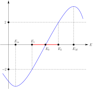
Figure 2: The discriminant $D(E)$ near the spectral band $B=[E_{1},E_{2}]$.

One easily infers from the definition of the transfer matrix that $D(E)$ is a real monic polynomial of degree $L$ in $-E$. Since it is positive on $(E_{0},E_{M}]$ we can write $D(E)=\prod_{j=1}^{L}|E-\mathcal{E}_{j}|$ where $\mathcal{E}_{j}=E_{0}$ for some $j$. Hence, we have

$$f(E)=\frac{{\rm d}}{{\rm d}E}\ln(D(E))=\sum_{j=1}^{L}\frac{1}{E-\mathcal{E}_{j}},$$

and

$$f^{\prime}(E)=-\sum_{j=1}^{L}\frac{1}{(E-\mathcal{E}_{j})^{2}}\leq-\frac{1}{(E-E_{0})^{2}}.$$

Since $E_{M}$ is a zero of $f$, for every $E\in(E_{0},E_{M})$ we can write

$$f(E)=-\int_{E}^{E_{M}}f^{\prime}(E^{\prime})\,{\rm d}E^{\prime}\geq\int_{E}^{E_{M}}\frac{1}{(E^{\prime}-E_{0})^{2}}\,{\rm d}E^{\prime}=\frac{1}{E-E_{0}}-\frac{1}{E_{M}-E_{0}}.$$

Using the fact that $D(E_{2})=2$ we get that for $E\in[E_{2},E_{M}]$

$$\ln\frac{D(E)}{2}=\ln D(E)-\ln D(E_{2})=\int_{E_{2}}^{E}f(E^{\prime}){\rm d}E^{\prime}\geq\ln\frac{E-E_{0}}{E_{2}-E_{0}}-\frac{E-E_{2}}{E_{M}-E_{0}}\geq\ln\frac{E-E_{0}}{E_{2}-E_{0}}-1,$$

from which we obtain

$$\frac{D(E)}{2}\geq\frac{E-E_{0}}{{\rm e}(E_{2}-E_{0})}.$$

Since $D(E)={\rm tr}(T(L,E))$ one has $\displaystyle\|T(L,E)\|\geq\frac{D(E)}{2}$ which ends the proof. $\Box$

5.2 Proof of $(4)\Rightarrow(2)$

We start by following the argument of Lemma 5.1 in [Las1]. Recall that $h_{{\rm per},L}$ denotes the periodized Hamiltonian of the sample, see Section 2.2.

For any $L$ we denote the bands of $\sigma_{L}={\rm sp}(h_{{\rm per},L})$ by $B_{\ell}=[E_{1,\ell},E_{2,\ell}]$, $\ell\in\{1,\ldots,L\}$, and by $D(L,E)$ the discriminant of $h_{{\rm per},L}$. We denote by $E_{0,\ell}\in B_{\ell}$ the zeros of $D(L,E)$ and by $E_{m,\ell}$, $\ell\in\{0,\ldots,L\}$, its local extrema, so that $E_{m,0}=-\infty$, $E_{m,\ell}\in[E_{2,\ell},E_{1,\ell+1}]$ for $\ell\in\{1,\ldots,L-1\}$ and $E_{m,L}=+\infty$. Finally, assume that $(L_{k})$, $\mu_{l}$ and $\mu_{r}$ are such that (4) holds, i.e.

$$G_{\rm Th}(L_{k},\mu_{l},\mu_{r})=\frac{|\sigma_{L_{k}}\cap(\mu_{l},\mu_{r})|}{2\pi(\mu_{r}-\mu_{l})}\to 0\quad\mbox{ as }\ k\to\infty.$$ (5.6)

The first step of the proof is to enlarge $\sigma_{L_{k}}$ in an appropriate way so that energies $E$ which are not in this enlarged spectrum are actually “far” from $\sigma_{L_{k}}$ (thus, by Proposition 5.4, $\|T(L_{k},E)\|$ will be large for these energies), while at the same time the measure of enlarged spectrum within $I=(\mu_{l},\mu_{r})$ remains small. The construction goes as follows. Let $(c_{k})$ be a sequence of positive numbers such that $c_{k}\to\infty$, $\displaystyle\frac{c_{k}}{L_{k}}\to 0$ and $c_{k}|\sigma_{L_{k}}\cap I|\to 0$. With

$$\ell_{-}=\max\{\ell\,:E_{0,\ell}<\inf(I)=\mu_{l}\}\quad\mbox{ and }\quad\ell_{+}=\min\{\ell\,:E_{0,\ell}>\sup(I)=\mu_{r}\},$$

set

$$\widetilde{B}_{\ell}=\left\{\begin{array}[]{ll}[E_{0,\ell}-c_{k}(E_{0,\ell}-E_{1,\ell}),E_{0,\ell}+c_{k}(E_{2,\ell}-E_{0,\ell})]&\text{if }\ell_{-}\leq\ell\leq\ell_{+};\\[8.0pt] B_{\ell}&\text{otherwise},\end{array}\right.$$

and define the enlarged spectrum by (see Figure 3)

$$S_{L_{k}}=\bigcup_{\ell=1}^{L_{k}}\widetilde{B}_{\ell}.$$

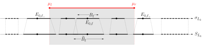
Figure 3: The enlarged spectrum $S_{L_{k}}$.

Note that for $\ell_{-}<\ell<\ell_{+}$ one has $E_{0,\ell}\in I$ and a simple analysis shows that

$$|\widetilde{B}_{\ell}\cap I|\leq c_{k}|B_{\ell}\cap I|,$$

while for $\ell=\ell_{\pm}$, taking Proposition 5.2 into account, we can write

$$|\widetilde{B}_{\ell}\cap I|\leq|\widetilde{B}_{\ell}|=c_{k}|B_{\ell}|\leq\frac{2\pi c_{k}}{L_{k}}.$$

In the other cases, one has

$$\widetilde{B}_{\ell}\cap I=B_{\ell}\cap I=\emptyset.$$

Thus, the overlap of the extended spectrum with the interval $I$ can be estimated as

$$|S_{L_{k}}\cap I|\leq\sum_{1\leq\ell\leq L}|\widetilde{B}_{\ell}\cap I| =\sum_{\ell_{-}<\ell<\ell_{+}}|\widetilde{B}_{\ell}\cap I|+|\widetilde{B}_{\ell_{-}}\cap I|+|\widetilde{B}_{\ell_{+}}\cap I|$$

$$\leq c_{k}\sum_{\ell_{-}<\ell<\ell_{+}}|B_{\ell}\cap I|+\frac{4\pi c_{k}}{L_{k}}$$

$$\leq c_{k}|\sigma_{L_{k}}\cap I|+\frac{4\pi c_{k}}{L_{k}}.$$

Our assumption on the sequence $(c_{k})$ ensures that the enlarged spectrum still satisfies

$$|S_{L_{k}}\cap I|\to 0.$$

Suppose now that $E\in I\setminus S_{L_{k}}$. Then $E\notin\widetilde{B}_{\ell}$ for any $\ell$ and hence must be in one of the intervals $(E_{2,\ell},E_{m,\ell}]$ with $E-E_{0,\ell}>c_{k}(E_{2,\ell}-E_{0,\ell})$ or in $[E_{m,\ell},E_{1,\ell+1})$ with $E_{0,\ell+1}-E>c_{k}(E_{0,\ell+1}-E_{1,\ell+1})$. In either case, it follows from Proposition 5.4 that

$$\|T(L_{k},E)\|\geq\frac{c_{k}}{{\rm e}}.$$

Since $\|T(L_{k},E)\|\geq 1$ for any $E$, we derive that, for all $E\in I$ and any $k$,

$$\|T(L_{k},E)\|\geq\frac{c_{k}}{{\rm e}}\left(1-{\mathbbm{1}}_{S_{L_{k}}}(E)\right)+{\mathbbm{1}}_{S_{L_{k}}}(E),$$ (5.7)

where ${\mathbbm{1}}_{S_{L_{k}}}$ denotes the characteristic function of the set $S_{L_{k}}$. Hence, for any $k$,

$$\int_{I}\|T(L_{k},E)\|^{-2}{\rm d}E\leq\left(\frac{{\rm e}}{c_{k}}\right)^{2}|I\setminus S_{L_{k}}|+|I\cap S_{L_{k}}|\leq\left(\frac{{\rm e}}{c_{k}}\right)^{2}|I|+|I\cap S_{L_{k}}|.$$

The last estimate yields

$$\lim_{k\to\infty}\int_{I}\|T(L_{k},E)\|^{-2}{\rm d}E=0,$$

and concludes the proof of $(4)\Rightarrow(2)$.

5.3 Proof of $(2)\Rightarrow(4)$

Again in this section $h_{{\rm per},L}$ denotes the periodized Hamiltonian of the sample acting on $\ell^{2}({\mathbb{Z}})$. The main part of the proof concerns fixed $L$ and we shall occasionally simplify the notation by omitting the $L$ dependence of various quantities.

We first introduce some notation. If $E$ is an interior point of the spectral band $B_{\ell}$ of $h_{{\rm per},L}$, then there exists a unique $k\in(0,\pi/L)$ such that $E=E_{\ell}(k)$. We write $k(E)$ for this unique $k$. The rotation number is the function defined as

$$\alpha(E)=\int_{-\infty}^{E}\left|k^{\prime}(\mathcal{E})\right|{\rm d}\mathcal{E},$$ (5.8)

where, by convention, we set $k^{\prime}(E)=0$ when $E$ is not an interior point of any spectral band. Since $k(E)$ is strictly monotone on each $B_{\ell}$ one easily gets that, for any $\ell$,

$$\int_{B_{\ell}}\left|k^{\prime}(\mathcal{E})\right|{\rm d}\mathcal{E}=\frac{\pi}{L}.$$

Hence, $E\mapsto\alpha(E)$ is strictly increasing on ${\rm sp}(h_{{\rm per},L})$ and constant on its complement. Thus, it defines a bijection from ${\rm sp}(h_{{\rm per},L})$ to $[0,\pi]$. We shall denote by $E(\alpha):[0,\pi]\to{\rm sp}(h_{{\rm per},L})$ its inverse and re-parametrize the Bloch waves by defining

$$u(\alpha,m)=u_{\ell}(k,m),\quad\mbox{for}\quad\alpha=\alpha(E_{\ell}(k)).$$

We note that for any $\ell\in\{1,\ldots,L\}$ and $k\in(0,\pi/L)$ one has

$$E^{\prime}(\alpha(E_{\ell}(k)))=\frac{1}{\alpha^{\prime}(E_{\ell}(k))}=\frac{1}{|k^{\prime}(E_{\ell}(k))|}=\left|E_{\ell}^{\prime}(k)\right|.$$ (5.9)

A fundamental result about the rotation number is the following estimate due to Deift and Simon [DS]; see also [ShSo].

Theorem 5.5

([DS], Theorem 1.4) For a.e. $E\in{\rm sp}(h_{{\rm per},L})$,

$$2\sin(\alpha(E))\alpha^{\prime}(E)\geq 1.$$

We shall only need a weaker version of it, namely the fact that

$$|\alpha^{-1}(\mathcal{A})|\leq 2|\mathcal{A}|,$$ (5.10)

for any measurable set $\mathcal{A}\subset[0,\pi]$.

We now state and prove two preparatory lemmas.

Lemma 5.6

$$\int_{0}^{\pi}\left(|u(\alpha,1)|^{2}+|u(\alpha,2)|^{2}\right){\rm d}\alpha=\frac{2\pi}{L}.$$

Proof.  Changing the variable of integration, we can write

$$\int_{0}^{\pi}\left(|u(\alpha,1)|^{2}+|u(\alpha,2)|^{2}\right){\rm d}\alpha=\sum_{\ell=1}^{L}\int_{0}^{\pi/L}\left(|u_{\ell}(k,1)|^{2}+|u_{\ell}(k,2)|^{2}\right)\alpha^{\prime}(E_{\ell}(k))|E_{\ell}^{\prime}(k)|{\rm d}k,$$

and Eq. (5.9) allows us to rewrite the right hand side of the last identity as

$$\int_{0}^{\pi/L}\left[\sum_{\ell=1}^{L}\left(|u_{\ell}(k,1)|^{2}+|u_{\ell}(k,2)|^{2}\right)\right]{\rm d}k=\int_{0}^{\pi/L}\left(\|\vec{u}_{\ell}(k,0)\|^{2}+\|\vec{u}_{\ell}(k,1)\|^{2}\right){\rm d}k=\frac{2\pi}{L}.$$

$\Box$

Lemma 5.7

1. $$\left|\left\{E\in{\rm sp}(h_{{\rm per},L})\,:\,|u(\alpha(E),1)|^{2}+|u(\alpha(E),2)|^{2}>\frac{4\pi}{L\epsilon}\right\}\right|\leq\epsilon.$$

2. $$\left|\left\{E\in{\rm sp}(h_{{\rm per},L})\,:\,\alpha^{\prime}(E)>\epsilon^{-1}\right\}\right|\leq\pi\epsilon$$

Proof.  (i) It follows immediately from Lemma 5.6 that the set

$$\mathcal{A}=\left\{\alpha\in[0,\pi]\,:\,|u(\alpha,1)|^{2}+|u(\alpha,2)|^{2}>\frac{4\pi}{L\epsilon}\right\}$$

is such that $|\mathcal{A}|\leq\frac{\epsilon}{2}$. The results thus follows from the Deift-Simon estimate (5.10).

(ii) Let $\mathcal{E}=\left\{E\in{\mathbb{R}}\,:\,\alpha^{\prime}(E)>\epsilon^{-1}\right\}$ and note that

$$\pi=\int_{-\infty}^{\infty}\alpha^{\prime}(E){\rm d}E\geq\frac{1}{\epsilon}|\mathcal{E}|.$$

$\Box$

Proof of Theorem 1.1, $(2)\Rightarrow(4)$. For a.e. $E\in{\rm sp}(h_{{\rm per},L})$, Proposition 5.3 and Eq. (5.9) yield

$$\|T(L,E)\|\leq 2L(|u(\alpha(E),1)|^{2}+|u(\alpha(E),2)|^{2})\alpha^{\prime}(E).$$

Let $\epsilon>0$. It follows from Lemma 5.7 that there exists $\Omega_{\epsilon}\subset{\rm sp}(h_{{\rm per},L})$ such that $|\Omega_{\epsilon}|\leq(1+\pi)\epsilon$ and

$$|u(\alpha(E),1)|^{2}+|u(\alpha(E),2)|^{2}\leq\frac{4\pi}{L\epsilon},\qquad\alpha^{\prime}(E)\leq\frac{1}{\epsilon},$$

for a.e. $E\in{\rm sp}(h_{{\rm per},L})\setminus\Omega_{\epsilon}$. Thus, for the same $E$, the estimate

$$\|T(L,E)\|\leq 2L\,\frac{4\pi}{L\epsilon}\,\frac{1}{\epsilon}=\frac{8\pi}{\epsilon^{2}},$$

holds. Hence, for any $L$, one has

$$\int_{\mu_{l}}^{\mu_{r}}\|T(L,E)\|^{-2}{\rm d}E \geq\int_{(\mu_{l},\mu_{r})\cap({\rm sp}(h_{{\rm per},L})\setminus\Omega_{\epsilon})}\|T(L,E)\|^{-2}{\rm d}E$$

$$\geq\frac{\epsilon^{4}}{64\pi^{2}}\big{(}|{\rm sp}(h_{{\rm per},L})\cap(\mu_{l},\mu_{r})|-|\Omega_{\epsilon}|\big{)}.$$ (5.11)

Suppose now that $(L_{k})$ is such that

$$\lim_{k\to\infty}\int_{\mu_{l}}^{\mu_{r}}\|T(L_{k},E)\|^{-2}{\rm d}E=0.$$

Then (5.11) gives

$$\limsup_{k\to\infty}|{\rm sp}(h_{{\rm per},L_{k}})\cap(\mu_{l},\mu_{r})|\leq|\Omega_{\epsilon}|\leq(1+\pi)\epsilon.$$

Since this holds for any $\epsilon>0$, we have

$$\lim_{k\to\infty}|{\rm sp}(h_{{\rm per},L_{k}})\cap(\mu_{l},\mu_{r})|=0,$$

and (4) follows.

Remark. The argument of Section 3.1 gives that

$$\limsup_{L\rightarrow\infty}\int_{I}\|T(L,E)\|^{-2}{\rm d}E\leq|{\rm sp}_{\rm ac}(h)\cap I|.$$

Combining this estimate with (5.11) one gets

$$\limsup_{L\rightarrow\infty}|{\rm sp}(h_{{\rm per},L})\cap I|\leq\frac{64\pi^{2}}{\epsilon^{4}}|{\rm sp}_{\rm ac}(h)\cap I|+(1+\pi)\epsilon.$$

Optimizing over $\epsilon$ one derives the bound (1.15) discussed at the end of Remark 7 after Theorem 1.1. A more refined optimization gives the better constant $C=5(4\pi^{4})^{1/5}\simeq 16.5$. These points will be further discussed in [BJLP2].

References

- [AJPP] Aschbacher, W., Jakšić, V., Pautrat, Y., and Pillet, C.-A.: Transport properties of quasi-free fermions. J. Math. Phys. 48, 032101 (2007).
- [Av] Avila, A.: On the Kotani-Last and Schrödinger conjectures. To appear in J. Amer. Math. Soc.
- [BSP] Ben Sâad, R., and Pillet, C-A.: A geometric approach to the Landauer-Büttiker formula. J. Math. Phys. 55, 075202 (2014).
- [BLS] Breuer, J., Last, Y., and Strauss, Y.: Eigenvalue spacings and dynamical upper bounds for discrete one-dimensional Schrödinger operators. Duke Math. J., 157, 425–460 (2011).
- [BJ] Bruneau, L., and Jakšić, V.: Unpublished.
- [BJP] Bruneau, L., Jakšić, V., and Pillet, C.A.: Landauer-Büttiker formula and Schrödinger conjecture. Commun. Math. Phys. 319, 501–513 (2013).
- [BJLP1] Bruneau, L., Jakšić, V., Last, Y., and Pillet, C.A.: Landauer-Büttiker and Thouless conductance. Commun. Math. Phys., online first, February 2015. DOI 10.1007/s00220-015-2321-0.
- [BJLP2] Bruneau, L., Jakšić, V., Last, Y., and Pillet, C.A.: What is absolutely continuous spectrum? In preparation.
- [BILP] Büttiker, M., Imry, Y., Landauer, R., and Pinhas, S.: Generalized many-channel conductance formula with application to small rings. Phys. Rev. B 31, 6207 (1985).
- [Ca] Carmona, R.: One dimensional Schrödinger operators with random or deterministic potentials: New spectral types. J. Funct. Anal. 51, 229–258 (1983).
- [CGM] Casati, G., Guarneri, I., and Maspero, G.: Landauer and Thouless conductance: a band random matrix approach. J. Phys. I France 7, 729 (1997).
- [CJM] Cornean, H.D., Jensen, A., and Moldoveanu, V.: A rigorous proof of the Landauer-Büttiker formula. J. Math. Phys. 46, 042106 (2005).
- [DS] Deift, P., and Simon, B.: Almost periodic Schrödinger operators III. The absolutely continuous spectrum in one dimension. Commun. Math. Phys. 90, 389–411 (1983).
- [ET] Edwards, J.T., and Thouless, D.J.: Numerical studies of localization in disordered systems. J. Phys. C: Solid State Phys. 5, 807–820 (1972).
- [GS] Gesztesy, F., and Simon, B.: The xi function. Acta Math. 176, 49–71 (1996).
- [GP] Gilbert, D.J., and Pearson, D.: On subordinacy and analysis of the spectrum of one dimensional Schrödinger operators. J. Math. Anal. 128, 30 (1987).
- [JLPa] Jakšić, V., Landon, B., and Panati, A.: A note on reflectionless Jacobi matrices. Commun. Math. Phys. 332, 827–838 (2014).
- [JOPP] Jakšić, V., Ogata, Y., Pautrat, Y., and Pillet, C.-A.: Entropic fluctuations in quantum statistical mechanics–an introduction. In Quantum Theory from Small to Large Scales. J. Fröhlich, M. Salmhofer, V. Mastropietro, W. De Roeck and L.F. Cugliandolo editors. Oxford University Press, Oxford, 2012.
- [Ko] Kotani, S.: Lyapunov indices determine absolutely continuous spectra of stationary random one-dimensional Schrödinger operators. In: Stochastic Analysis, K. Itÿo, ed., Amsterdam: North-Holland, 225–247 (1984).
- [KR] Krutikov, D., and Remling, C.: Schrödinger operators with sparse potentials: asymptotics of the Fourier transform of the spectral measure. Commun. Math. Phys. 223, 509–532 (2001).
- [La] Landauer, R.: Electrical resistance of disordered one-dimensional lattices. Phil. Mag. 21, 863 (1970).
- [Lan] Landon, B.: Master’s thesis, McGill University (2013).
- [Las1] Last, Y.: Conductance and spectral properties. Ph.D. Thesis, Technion (1994).
- [Las2] Last, Y.: On the measure of gaps and spectra for discrete 1D Schrödinger operators. Commun. Math. Phys. 149, 347–360 (1992).
- [Las3] Last, Y.: A relation between a.c. spectrum of ergodic Jacobi matrices and the spectra of periodic approximants. Commun. Math. Phys. 151, 183–192 (1993).
- [LaS] Last, Y., and Simon, B.: Eigenfunctions, transfer matrices, and absolutely continuous spectrum of one-dimensional Schrödinger operators. Invent. Math. 135, 329 (1999).
- [MMG] Maslov, V.P., Molchanov, S.A., and Gordon, A. Ya.: Behavior of generalized eigenfunctions at infinity and the Schrödinger conjecture. Russian J. Math. Phys. 1, 71 (1993).
- [N] Nenciu, G.: Independent electrons model for open quantum systems: Landauer-Büttiker formula and strict positivity of the entropy production. J. Math. Phys. 48, 033302 (2007).
- [Re] Remling, C.: The absolutely continuous spectrum of Jacobi matrices. Annals of Mathematics 174, no 1., 125-171 (2011).
- [ShSo] Shamis, M., and Sodin, S.: On the measure of the absolutely continuous spectrum for Jacobi matrices. J. Spectr. Theory 1, 349–362 (2011).
- [Si1] Simon, B.: Bounded eigenfunctions and absolutely continuous spectra for one dimensional Schrödinger operators. Proc. Amer. Math. Soc. 124, 3361 (1996).
- [Si2] Simon, B.: Schrödinger semigroups. Bulletin AMS 7, 447 (1982).
- [Si3] Simon, B.: Szegö’s Theorem and Its Descendants. Spectral theory for Perturbations of Orthogonal Polynomials. M.B. Porter Lectures. Princeton University Press, Princeton, NJ, 2011.
- [Si4] Simon, B.: Kotani theory for one dimensional stochastic Jacobi matrices. Commun. Math. Phys. 89, 227–234 (1983).
- [Si5] Simon, B.: Orthogonal polynomials with exponentially decaying recursion coefficients. Probability and Mathematical Physics (eds. D. Dawson, V. Jakšić and B. Vainberg), CRM Proc. and Lecture Notes 42, 453–463 (2007).
- [Y] Yafaev, D.R.: Mathematical scattering theory. General theory. Translated from the Russian by J. R. Schulenberger. Translations of Mathematical Monographs 105. American Mathematical Society, Providence, RI, 1992.