Microlensing events from the 11-year observations of the Wendelstein Calar Alto Pixellensing Project

Abstract

We present the results of the decade-long M31 observation from the Wendelstein Calar Alto Pixellensing Project (WeCAPP). WeCAPP has monitored M31 from 1997 till 2008 in both $R$- and $I$-filters, thus provides the longest baseline of all M31 microlensing surveys. The data are analyzed with the difference imaging analysis, which is most suitable to study variability in crowded stellar fields. We extracted light curves based on each pixel, and devised selection criteria that are optimized to identify microlensing events. This leads to 10 new events, and sums up to a total of 12 microlensing events from WeCAPP, for which we derive their timescales, flux excesses, and colors from their light curves. The color of the lensed stars fall between $(R-I)$ = 0.56 to 1.36, with a median of 1.0 mag, in agreement with our expectation that the sources are most likely bright, red stars at post main-sequence stage. The event FWHM timescales range from 0.5 to 14 days, with a median of 3 days, in good agreement with predictions based on the model of Riffeser et al. (2006).

1 Introduction

Almost four decades after revealing evidences for dark matter in galaxies (Rubin et al., 1980), its nature is still unknown. Dark matter can be smoothly distributed, e.g. the weakly interacting massive particles (WIMPs), or in compact form. Since dark matter does not emit light, the best way to study it is through gravitational interaction. Paczynski (1986) was the first to conceive the idea of gravitational microlensing as a method to detect massive compact halo dark matter (MACHO). Based on his calculation, the optical depth, i.e. at any time the probability of a source to be closer along the line of sight to a foreground lens than the lens’ Einstein angle therefore to be magnified by more than 1.34, is of order 10^-6 towards Magellanic Clouds. This has motivated several campaigns to search for microlensing towards dense stellar fields, see e.g. the review by Moniez (2010). The first microlensing events were reported by the MACHO (Alcock et al., 1993), EROS (Aubourg et al., 1993), and OGLE (Udalski et al., 1993) teams, with MOA (Muraki et al., 1999) joining later on. In their 5.7-year survey data, the MACHO team has announced 13 microlensing events towards the Large Magellanic Cloud (Alcock et al., 2000), while a later analysis (Bennett, 2005) showed that 1 of them is a true variable star and 2 of them are likely to be variables from a simple likelihood analysis. This leaves 10 of them to be plausible microlensing events, and gives a MACHO halo fraction of 16% for MACHO masses between 0.1 - 1 M_⊙ (Bennett, 2005). The EROS-1 and EROS-2 surveys resulted in a MACHO halo fraction of less than 8% for MACHO mass $\sim$ 0.4 M_⊙, and ruled out MACHOs with masses between 0.6$\times$10^-7 and 15 M_⊙ as a major component of the Milky Way halo (Tisserand et al., 2007). Analyzing the OGLE phase II and III data, Wyrzykowski et al. (2010,2011a,2011b) concluded that microlensing events towards the Large and Small Magellanic Cloud can be reconciled with self-lensing by stars alone, i.e. without requiring compact halo objects in the Milky Way halo. Later on, Besla et al. (2013) studied the tidal streams between the Magellanic Clouds and used theoretical modeling to show that the microlensing signal can be reproduced by the stars in the stream, though their modeling requires further verification. Besla et al. (2013) outlined several observational tests to verify their theoretical modeling, e.g. the sources of the microlensing events are low-metallicity SMC stars, the sources have high velocities relative to the LMC disk stars, and the presence of a very faint stellar counterpart to the Magellanic Stream and Bridge (surface brightness $>$ 34 mag/arcsec² in V-band).

In contrast to this, Calchi Novati et al. (2013) recently re-analyzed the OGLE and EROS data and found that some of the OGLE events can be attributed to halo lensing. The inconclusive results can be partially attributed to the fact that, by monitoring the Magellanic Clouds we can only sample a small fraction of the Milky Way halo. In order to have a census of the Milky Way halo, we need targets that are distributed along different lines-of-sights through the Milky Way halo. Other than the Milky Way, we could monitor a nearby spiral galaxy, for which we can have a complete view of its dark halo.

An alternative dense stellar target for a microlensing search for MACHOs is M31, as proposed by several authors (Crotts, 1992; Baillon et al., 1993; Jetzer, 1994). The advantage of M31 is twofold. First, we can have multiple lines-of-sight through a dark halo towards M31, in contrast to the single line-of-sight towards the Magellanic Clouds due to our location in the Milky Way. The second advantage is that one does not only probe the Milky Way halo, but also that of M31. The structure of M31 is well known: with an inclination angle of 77^o (Walterbos & Kennicutt, 1987), we expect to see an asymmetry of the microlensing event rate between the near- and far-side of M31 disk. Such an asymmetry can however also originate from extinction along different sight-lines caused by dust. This has indeed been observed in the density distribution of variables from the POINT-AGAPE survey (An et al., 2004) and from the WeCAPP (Fliri et al., 2006). To be able to account for this dust effect, we have studied the dust properties of M31 (Montalto et al., 2009) and derived an extinction map across the disk of M31, which can be used for quantifying detection efficiencies. Microlensing in M31 differs from the Magellanic Clouds, because at the distance of M31 (770 kpc, Freedman & Madore, 1990), most of the sources for possible microlensing events are not resolved, and each pixel of a CCD image contains up to hundreds of stars. Instead of monitoring individual resolved stars, one has to monitor pixel light curves and their variations towards dense stellar fields. The sources of microlensing events are usually not resolved before and after the high magnification phases and their “baseline fluxes” are thus unknown. In most cases the magnified source (at least at maximum magnification) appears as a resolved object. However, in order to achieve exquisite photometry in such crowded fields, we thus perform difference image analysis and search for microlensing events at the position of each individual pixel. In order to extract light curves at the position of each individual pixel, we use a PSF constructed from resolved sources in the image to perform PSF photometry and obtain pixel light curves.

The theoretical aspect of pixel lensing has been laid down by Gould (1996) under small impact parameter assumption. Riffeser et al. (2006) reformulated this theory in a more general context.

The first microlensing events towards M31 were reported by the VATT/Columbia microlensing survey. They put the idea of Crotts (1992) into practice (Tomaney & Crotts, 1996) and presented 6 microlensing events discovered by the joint observations of the Vatican Advanced Technology Telescope (VATT) and the KPNO 4m telescope taken during 1994 and 1995 (Crotts & Tomaney, 1996). Their observations continued from 1997 to 1999, with the VATT and the 1.3m telescope at the MDM observatory. With additional data from the Isaac Newton Telescope, they presented 4 probable microlensing events out of their 3 year data (Uglesich et al., 2004). At the same time, Ansari et al. (1997) also launched the Andromeda Gravitational Amplification Pixel Experiment (AGAPE); they observed M31 with the 2m telescope Bernard Lyot (TBL) in the French Pyrenees in 1994 and 1995, which led to the discovery of one bright, short microlensing event (Ansari et al., 1999). Following AGAPE, the Pixel-lensing Observations with the Isaac Newton Telescope-Andromeda Galaxy Amplified Pixels Experiment (POINT-AGAPE) has monitored M31 from 1999 to 2001; their first microlensing event was announced in Aurière et al. (2001), accompanied by three more in Paulin-Henriksson et al. (2002); Paulin-Henriksson et al. (2003); another 3 were reported by Calchi Novati et al. (2003) with additional data from the 1.3m telescope at the MDM observatory in 1998-1999. The full POINT-AGAPE data were analyzed with 3 different pipelines based at Cambridge, Zürich, and London, where 3 (Belokurov et al., 2005), 6 (Calchi Novati et al., 2005), and 10 events (Tsapras et al., 2010) were reported by the different nodes, respectively.

Using the same INT data, the Microlensing Exploration of the Galaxy and Andromeda (MEGA) survey has presented 14 events (de Jong et al., 2006). At the same time, the Nainital Microlensing Survey employed the 1.04m Sampurnanand Telescope in India to observe from September 1998 until February 2002. They have extracted 1 microlensing event from the 4-year data (Joshi et al., 2005). More recently, the Pixel Lensing Andromeda collaboration (PLAN) carried out observations using the 1.5m Loiano telescope located in Italy (Calchi Novati et al., 2007) and reported 2 events in their data collected in 2007 (Calchi Novati et al., 2009). They further incorporated observations from the 2m Himalayan Chandra Telescope (HCT) taken in 2010 and reported another event (Calchi Novati et al., 2014). In the mean time, the Pan-STARRS 1 collaboration conducted a high-cadence, long-term Andromeda monitoring campaign (PAndromeda) utilizing its wide-field ($\sim$ 7 deg²) camera. Based on its first year data, Lee et al. (2012) have reported 6 events in the central 40”$\times$40” area, with the promises to detect more events taking advantage of the larger survey area and higher cadence from Pan-STARRS 1.

It is worth to note that previous M31 microlensing event identifications may suffer from contaminations by variables. For example, Crotts & Tomaney (1996) suspected that part of their events are contaminated by long-period red supergiant variables. Despite the efforts of various campaigns, the MACHO fraction at the mass range of 0.1-1$M_{\odot}$ is still under debate (see Calchi Novati, 2012, for a detailed discussion). For example, the POINT-AGAPE collaboration has reported evidence for MACHO signal (Calchi Novati et al., 2005), while the MEGA collaboration (de Jong et al., 2006) on the contrary concluded that their events can be fully explained by self-lensing.

Due to the small number of reported events, the origin of M31 microlensing remains an open issue. In this study, we aim to increase the number of microlensing detections and suppress contaminations by variables with long-term observations of the M31 bulge. This paper is structured as follows. In section 2 we present the observations of our long-term survey. Our data reduction is outlined in section 3, followed by the event detection in section 4. The analysis of these events are shown in section 5. A discussion of our events, as well as results from previous M31 microlensing surveys are presented in section 6, with a summary and prospects in section 7.

2 Observations

Season	Observatory	R-band				I-band				R or I-band				R or I-band
		F1	F2	F3	F4	F1	F2	F3	F4	F1	F2	F3	F4	F1 or F2 or F3 or F4
1997 1998	WS	36	7	1	4	33	7	0	3	37	7	1	4	38
1998 1999	WS	33	1	1	1	28	1	1	1	33	1	1	1	33
	WS	64	0	0	0	60	0	0	0	65	0	0	0	65
	CA	89	0	0	0	84	0	0	0	95	0	0	0	95
1999 2000	WS or CA	128	0	0	0	124	0	0	0	134	0	0	0	134
	WS	75	0	16	0	68	0	15	0	75	0	16	0	75
	CA	106	107	107	107	89	89	89	89	106	107	107	107	107
2000 2001	WS or CA	153	107	119	107	137	89	101	89	153	107	119	107	154
	WS	106	0	23	0	93	0	21	0	106	0	23	0	106
	CA	134	136	136	136	119	119	119	119	137	137	137	137	137
2001 2002	WS or CA	200	136	148	136	176	119	129	119	201	137	148	137	201
	WS	27	11	16	11	24	10	17	12	27	11	18	12	45
	CA	7	7	7	7	6	6	6	6	7	7	7	7	7
2002 2003	WS or CA	34	18	23	18	30	16	23	18	34	18	25	19	52
2003 2004	WS	35	24	29	31	33	21	26	29	35	24	29	32	69
2004 2005	WS	25	23	26	25	19	16	19	19	26	23	26	25	47
2005 2006	WS	30	25	28	28	26	20	22	23	32	26	28	28	71
2006 2007	WS	107	106	103	103	48	45	46	47	107	108	104	103	124
2007 2008	WS	62	56	52	58	36	35	35	38	63	58	55	61	92
total	WS	600	253	295	261	468	155	202	172	606	258	301	266	765
total	CA	336	250	250	250	298	214	214	214	345	251	251	251	346
total	WS or CA	843	503	530	511	690	369	402	386	855	509	536	517	1015

Table 1: The number of analyzed nights per year during the 11 WeCAPP seasons. Note that from 1999 until 2002 we used both telescopes at Wendelstein (WS) and Calar Alto (CA). A season is defined to last from May 1^th until 30^th April of the next year. The total amount of observed nights are 1015 nights out of 11 years. A total of 4,432 stacked frames were analyzed in both filters and 4 fields.

WeCAPP continuously monitored M31 from August 1997 until March 2008 using the Wendelstein 0.8m telescope (Riffeser et al., 2001). The data were initially taken with a TEK CCD with 1,024$\times$1,024 pixels with a field-of-view of 8.3$\times$8.3 arcmin² pointing at the bulge of M31, optimally on a daily basis in both R- and I-filters. Following the suggestions of Tomaney & Crotts (1996) and Han & Gould (1996), we pointed to the far side of the M31 disk (F1 in Fig. 1), where the halo lensing probability is maximized. From June 1999 to December 2002 we collected additional data using the 1.23 m (17’.2$\times$17’.2 FOV) telescope at Calar Alto Observatory in Spain to increase the time sampling. This provided a FOV which is four times the Wendelstein FOV, and enabled us to survey the major part of the M31 bulge. After 2002, we used the Wendelstein telescope solely to mosaic the full Calar Alto field-of-view with four pointings, as indicated in Fig. 1.

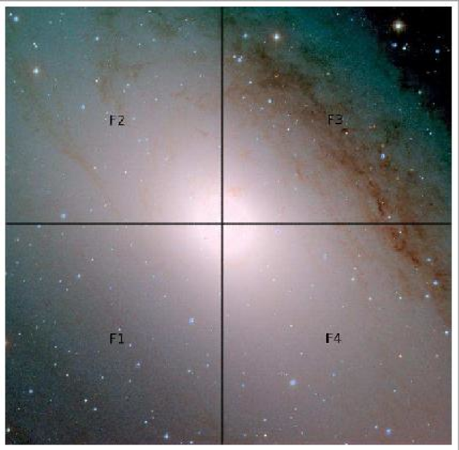
Figure 1: M31 composite image ($V$-, $R$-, and $I$-band) of the observed fields F1 to F4, taken at Calar Alto Observatory during the 2000/2001 season. The black lines mark the positions of fields F1 to F4. The Calar Alto camera covers all four fields simultaneously. Field F1 was observed during all 11 campaigns from September 1997 until March 2008.

The amount of observations taken in the four pointings differs significantly during the 11 seasons. Fig. 2 shows a histogram of the number of observed nights by WeCAPP. The most complete seasons are 2000/2001 and 2001/2002 with joint observations from both Wendelstein and Calar Alto (see also Table 1).

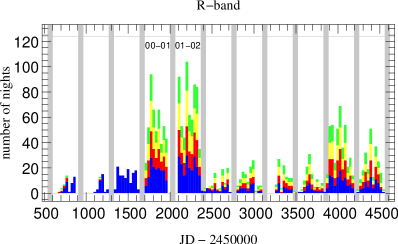
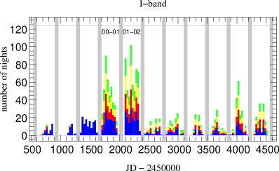
Figure 2: Histogram of the number of analyzed nights. The 4 different fields F1, F2, F3, F4 are colored blue red, yellow and green, respectively. Periods marked in gray show the 61 days (from $1^{st}$ April to $31^{st}$ May) during which M31 can hardly be observed (see also Table. 1). Our most complete seasons (2000/2001 and 2001/2002) are marked with the texts “00-01” and “01-02”.

To have an overview of the observing cadence, we show the daily sampling in Fig. 3. Thanks to the joint observations at Wendelstein and Calar Alto, we achieved an average time coverage for F1 in R of 42% during the 2000/2001 season (peaking in August 2000 with 90% on JD $\sim$ 2451770) and an average time coverage of 55% during the 2001/2002 season, reaching more than 93% in 3 months (July and October 2001, and January 2002, around JD $\sim$ 2452110, 2452200 and 2452290, respectively). During the 11 seasons, we have obtained a total sampling efficiency of 14.9% in $R$ and 11.5% in $I$, with 11.3% for $R$ and $I$ combined for all fields (F1-F4), which means that in 11.3% of the nights we have both $R$ and $I$ observations.

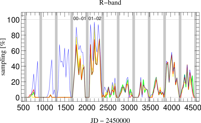
Figure 3: Daily sampling of the 4 different fields F1, F2, F3, F4 are colored in blue, red, yellow and green, respectively. Periods marked in gray show the 61 days (from $1^{st}$ April to $31^{st}$ May) during which M31 can hardly be observed. See also Table. 1. The two seasons with the highest sampling are 2000/2001 and 2001/2002, i.e. those seasons where we could combine Wendelstein with Calar Alto data.

However, not all images have the same quality. Rather than quantifying the fraction of nights we have observed through the 11 seasons we would like to have (as a function of location in M31) the fraction of nights where the noise is below a certain threshold. For this reason, we empirically chose a noise limit of the minimum S/N of 8.9 for our faintest event, i.e. 0.73 $\times$ 10^-5 Jy/8.9, which corresponds to the 8.9$\sigma$ detection criterion we present in section 4. For pixels with noise levels above this value, the lensing signal would mix with the high noises and could not be detected. Hence these pixels cannot be used for the detection. The sampling thus depends on the $x$ and $y$ position of the pixel, as well as the observation time $t$, which we denote as $<S$($x,y,t$)$>$. In Fig. 4, we show the area having a noise smaller than our noise limit for every observed night. By averaging over time $t$, we will get the positional dependence as shown in Fig. 5.

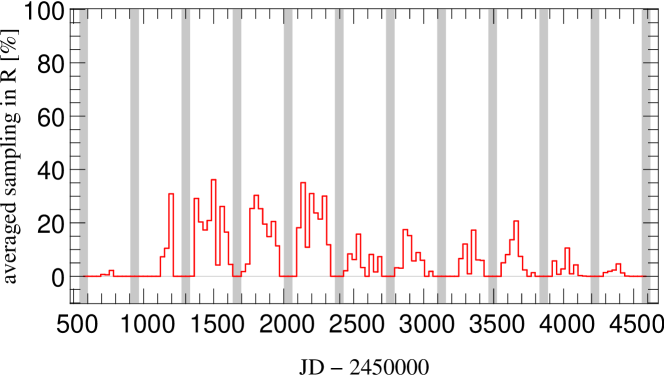
Figure 4: Sampling in $t$ averaged over $x$ and $y$ $<\mathrm{S}(x,y,t)>_{xy}$

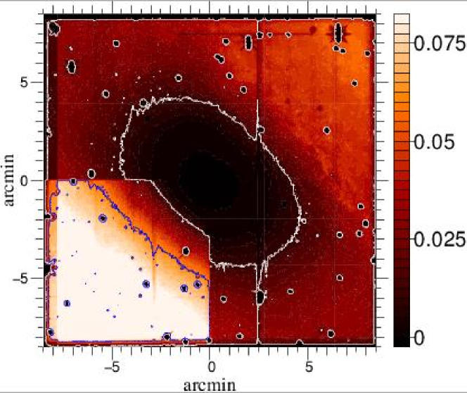
Figure 5: Sampling in $(x,y)$ averaged over time $<\mathrm{S}(x,y,t)>_{t}$. Color levels range from 0% to 10%; the two contour levels show 1% and 5%, respectively. 58 arcmin² are well sampled by more than 5% of the 11 year survey. 220 arcmin² are well sampled by more than 1%.

3 Data reduction

We process the data using our customized pipeline MUPIPE (Gössl & Riffeser, 2002), where standard reduction processes – such as bias subtraction, treatment of bad pixels, flat-fielding, cosmic ray removing – are performed with per pixel error propagation. To identify unresolved variables, we employ the difference imaging analysis (DIA) proposed by Alard & Lupton (1998), which enables us to detect variables with amplitudes at the photon noise level and to measure their flux excesses relative to high signal-to-noise reference images.

After the difference imaging, we perform PSF photometry on each pixel in the following manner. We first extract the PSF profile from several isolated, bright and unsaturated reference stars. Then we fit this PSF to all pixels to generate light curves of varying sources identified in the difference images. The flux of the source is estimated by integrating the count rates over the area of the PSF.

The results from a subset of data of this project have been presented in Riffeser et al. (2003, 2008) and partially contributed to Calchi Novati et al. (2010). In addition to the original microlensing targets, the high cadence observations also yielded a sample of more than 20,000 variables in the bulge of M31 (Fliri et al., 2006) and 91 candidate novae (Pietsch et al., 2007; Lee et al., 2012).

4 Event detection

Paczynski (1986) provided an analytic formula to describe the amplification of a microlensing event:

$$A(t)=\frac{u^{2}+2}{u\sqrt{u^{2}+4}},\quad u=\sqrt{\frac{(t-t_{0})^{2}}{t_{\mathrm{E}}^{2}}+u_{0}^{2}},$$ (1)

where $t_{0}$ is the time of maximum amplification, $t_{\mathrm{E}}$ is the Einstein ring crossing time, $u_{0}$ is the impact parameter in units of the Einstein ring radius. The light curve (or the measured flux as a function of time) of the microlensing event can thus be expressed as:

$$F(t)=F_{0}[A(t)-1]+B,$$ (2)

where $F_{0}$ is the un-lensed flux and $B$ is the blending within the PSF.

This conventional microlensing light curve formula is highly degenerate in $t_{\mathrm{E}}$ and $u_{0}$ for microlensing events towards M31, because one can not resolve the source anymore. For M31 microlensing, the only observables are the flux excess ${\Delta_{F}}$ and the event time-scale $t_{\mathrm{FWHM}}$. Gould (1996) has derived the pixel-lensing light curve formula in the context of high magnification. Riffeser et al. (2006) further revised the microlensing light curve formula by Gould (1996), such that microlensing light curves with moderate magnifications can be well-described as well. The formula of pixel-lensing light curve from Riffeser et al. (2006) is expressed as:

$${\Delta_{F}}(t)\approx F_{\mathrm{eff}}\left[\frac{12(t-t_{0})^{2}}{t_{\mathrm{FWHM}}^{2}}+1\right]^{-1/2}+B$$ (3)

where $F_{\mathrm{eff}}$ is the effective flux, which for high magnifications is approximated by the flux excess $F_{\mathrm{eff}}\equiv F_{0}/u_{0}\approx\Delta_{F}$. Since Paczynski (1986) was the first to present the simple analytical form of microlensing light curve as equation (2), we refer to equation (2) as Paczynski-fit throughout this paper. Since Gould (1996) was the first to introduce the approximated form of microlensing light curve as equation (3), we refer to equation (3) as Gould-fit throughout this paper.

We use equation (3) to identify microlensing events. The microlensing event detection is performed on the light curve of each pixel (based on the aforementioned PSF photometry) with several successive criteria. Compared to Riffeser et al. (2003), we introduce additional criteria to avoid human interaction during the selection process. We now describe our criteria; an overview of the number of pixel light curves passing each criterion is listed in Table 2.

	criterion	number	left LCs from I	colors in Fig. 6
I	Analyzed LCs with $>$ 50 data points	3,872,240	100.0%
II	Three consecutive 3$\sigma$ in $R$	719,628	18.6%
III	$\chi_{R}<1.5$ and $\chi_{I}<2.1$	152,753	3.9%	yellow
IV	$(S/N)>8.9$ in $R$ and maximum with good PSF	2,247	0.5%	black
V	$-1.5\geq E_{R}^{peak}\leq 1.5$	1,379	10.4%	green
VI	$t_{\mathrm{FWHM}}<1000$d	63	16.8%	blue
VII	$samp^{t<t_{0}}_{R}>$0.18 and $samp^{t>t_{0}}_{R}>$0.08 and
	$samp^{t<t_{0}}_{I}>$0.18 and $samp^{t>t_{0}}_{I}>$0.08	12	9.3%	red

Table 2: Selection criteria for the 11 year data taken between MJD = 685.5 and 4535.3. In the 3rd column we show how applying each criterion (II, III, IV, V, VI, VII) to the 3,872,240 light curves (criterion I) reduces the filtered light curves.

• Criterion I is applied to exclude pixel light curves which have too few data points to make them worth analyzing. Hence we exclude light curves with less than 50 data points in either R- or I-filters. This leaves us with 3,872,240 light curves.

• Criterion II identifies varying sources warrant for further analysis. We preselect variable pixel light curves with at least three consecutive 3$\sigma$ outliers in the R-filter.

• Criterion III is designed to find microlensing light curves with good $\chi^{2}$. We select pixel light curves that are well described by microlensing light curves. We use the microlensing light curve in equation (3) with some modifications:

  $${\Delta_{F}}(t)\approx F_{\mathrm{eff}}\left[\frac{12(t-t_{0})^{2}}{\left(t_{\mathrm{fit}}^{2}+0.5\right)^{2}}+1\right]^{-1/2}+c$$ (4)

  where we set $t_{\mathrm{fit}}\equiv\sqrt{t_{\mathrm{FWHM}}-0.5}$, hence the full width half-maximum event timescale is always greater than or equal to 0.5 day. We use $t_{\mathrm{fit}}$ instead of $t_{\mathrm{FWHM}}$ to avoid un-physically small $t_{\mathrm{FWHM}}$ due to limited time resolution (up to half day) of our observation. The term $c$ takes into account the shift of the baseline flux by a constant in cases for which there is a variable source spatially close to the microlensing event and data of these variable phases enter the reference image.

  We then filter out light curves with a $\chi_{k}\equiv\sqrt{\chi_{k}^{2}}$ (where $\chi^{2}_{\mathrm{k}}$ is the total $\chi^{2}$ divided by the degrees of freedom $k$) larger than 1.5 in the R band and larger than 2.1 in the I band. This is less strict than the value we used in (Riffeser et al. 2003). The allowed $\chi_{\mathrm{k}}$ in I is slightly higher than R, because the noise level is increased by unaccounted systematics such as the detector fringing and nearby variable stars in the I band.

• Criterion IV evaluates whether a high flux excess relative to the baseline is more likely caused by random noise or due to a true microlensing signal. We consider the S/N of such a high flux excess measurement, $\mathrm{SN}_{i}\equiv\frac{\Delta_{\mathrm{con},i}}{\sigma_{i}}$, where the flux offset is $\Delta_{\mathrm{con},i}\equiv y_{i}-c$, $y_{i}$ is the $i$th flux measurement at time $t_{i}$ and $\sigma_{i}$ is the error of the flux measurement. We take into account the probability of such a high flux excess measurement being close to the maximum of a microlensing light curve fit $p_{\mathrm{fit},i}\propto\exp\left(-\frac{\Delta_{\mathrm{fit},i}^{2}}{2\sigma_{i}^{2}}\right)$, where the flux offset is $\Delta_{\mathrm{fit},i}\equiv y_{i}-\Delta_{F}(t_{i})$, and $\Delta_{F}(t_{i})$ is the model flux at time $t_{i}$ according to Equation (4). We also take into account the probability of such a high flux excess measurement being at the constant baseline $p_{\mathrm{con},i}\propto\exp\left(-\frac{\Delta_{\mathrm{con},i}^{2}}{2\sigma_{i}^{2}}\right)$. We then combine these three factors and define the S/N probability (SNP):

  $$\mathrm{SNP}_{i}=\mathrm{SN}_{i}\times p_{\mathrm{fit},i}\times\left(1-p_{\mathrm{con},i}\right)$$ (5)

  This ensures that light curves that have high $S/N$ outliers, that are outside the time interval of the microlensing event, get a lower weight.

  To avoid multiple detections of the same microlensing signal in neighboring pixels, we only use the pixel with good PSF detections to evaluate SNP_i, i.e. where the PSF fit has a minimum in $\chi^{2}$ with respect to neighboring pixels.

  We empirically require one data point in the light curve to have a SNP_i larger than 8.9 in the R band to efficiently reject faint variable sources.

• Criterion V quantifies the temporal correlations of the model-data mismatch (best-fit microlensing light curve vs. measured light curve) and enables us to reject intrinsic variable sources more efficiently.

  We combine the probabilities for positive $p^{+}_{i}$ or negative flux offsets $p^{-}_{i}$ from the best-fit microlensing light curve, and assign positive values for consecutive data points that are always on the same side (either above or below) of the best-fit model light curve. For consecutive data points alternating along the best-fit model light curve, we assign negative values. We then define the energy of a potential microlensing light curve as

  $$E\equiv\frac{\pi}{\sqrt{n}}\sum_{i=1}^{n-1}p^{+}_{i}p^{+}_{i+1}+p^{-}_{i}p^{-}_{i+1}-p^{+}_{i}p^{-}_{i+1}-p^{-}_{i}p^{+}_{i+1}$$ (6)

  where $n$ is the number of data points and the probabilities are defined as $p^{+}_{i}\equiv 0.5\left[1+\mathop{\rm erf}\nolimits\left(\sqrt{\frac{\Delta_{\mathrm{fit},i}^{2}}{2e_{i}^{2}}}\right)\right]$ and $p^{-}_{i}\equiv 1-p^{+}_{i}$.

  For a random process the distribution of $E$ is a Gaussian with an expectation value of zero and a standard deviation of one.

  We derive the energy $E^{20}$ using the $n=20$ closest data points to $t_{0}$ in the R-band. We find empirically that a value between -1.5 and 1.5 efficiently rejects periodic variables and allows to skip the previously used by-eye detection in Riffeser et al. (2003).

• Criterion VI filters out long-periodic variables. Since our light curves span a baseline of 11 years, contaminations from the long-periodic variables are less severe than any of the previous campaigns. We inspected the candidate light curves and found that false detection from systematics and moving objects are having timescales longer than 1000 days. Hence we are able to empirically increase the upper $t_{\mathrm{FWHM}}$-limit for micrlensing searches to 1000 days (compared to, e.g. $t_{\mathrm{FWHM}}<$ 20 days in Riffeser et la. 2003). With this criterion we also filter out objects with proper motion. A moving object that passes through the field with constant angular velocity will cause variabilities at some (stationary) pixels that can mimic microlensing signals. These proper motion objects can of course be excluded by inspecting postage stamps, but we would like to have a completely automatic selection here.

• Criterion VII rejects light curves which look like microlensing events from their overall light curves but which are not well sampled close to the light curve maximum, hence could be variable sources. The contaminations are mostly from novae, e.g. not well sampled in their rising parts.

  We define the sampling quality for the falling and rising parts of each light curve within $(t_{0}-15\,\mathrm{days},t_{0})$ and $(t_{0},t_{0}+15\,\mathrm{days})$. The contribution of a single data point is then calculated by integrating the model light curve within $(t_{i}-0.5\,\mathrm{days},t_{i}+0.5\,\mathrm{days})$. As sampling criteria we require a total sampling of the area under the light curve of at least 18% on the rising part of the light curve and of at least 8% on the falling side in the R and I band.

In the 4^th column of Table 2 we show how applying each criterion (II, III, IV, V, VI, VII) to the 3,872,240 light curves (criterion I) reduces the filtered light curves. For example, 152,753/3,872,240$\sim$3.9% light curves that pass criterion III. Less efficient criteria show a high percentage of remaining light curves while efficient criteria filter out more light curves. Therefore the criterion IV is our most efficient criterion. In the 3rd column we show how applying each criterion (II, III, IV, V, VI, VII) to the 3,872,240 light curves (criterion I) reduces the filtered light curves.

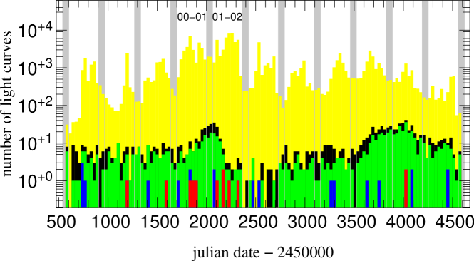
Figure 6: Histogram of the number of light curves passing different detection criteria. Our most complete seasons (2000/2001 and 2001/2002) are marked with “00-01” and “01-02”. Yellow: $\chi$-limit (III). Black: $(S/N)$ constraint and good PSF (IV) at light curve maximum. Green: Energy criterion for the 20 closest data points to the maximum (V). Blue: timescale constraint (VI). Red: sampling criterion for the closest data points to the maximum (VII). In the end we are left with 12 microlensing events detected (see Table 2 for details). Eight of them took place during the two best observing seasons 2000/2001 and 2001/2002.

Fig. 6 shows the $t_{0}$ distribution of all pixel light curves under analysis. The colored histograms show how the number of light curves is reduced after each criterion. The total numbers correspond to those given in Table 2.

Because of large dome seeing and an inappropriate auto-guiding system, photometric errors are largest during the first season (1997/98). During the second season (1998/99) we were able to decrease the FWHM of the PSF by a factor of two, and therefore the photometric scatter also became smaller.

The vast majority of our microlensing events are detected between 2000/2001 and 2001/2002 seasons, where we have employed the Calar Alto telescope and the cadence is high. This implies that deeper images with larger telescope along with densely sampled observations are crucial to detect microlensing events. Our observations in other seasons are pivotal as well, as they serve the purpose to rule out contamination from variables.

Fig. 7 shows the properties of the 719,628 light curves passing criterion II. Since the major contaminations to microlensing detections are variables and novae, we over-plot the 23,001 variable sources published in Fliri et al. (2006) in magenta and the 91 novae in Lee et al. 2012 in blue. In Fig. 7 it is clear that criterion III and IV are efficient to filter out these two major contamination sources.

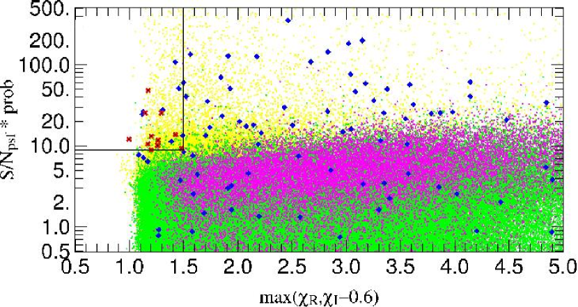
Figure 7: Criterion III and IV reduce the light curves from 719,628 (green) to 2247, as shown in the box on the upper left side. The light curves which do no pass criterion VI are marked in yellow. We show the 23,001 variables published in the WeCAPP variable star catalogue from Fliri et al. (2006) in magenta, as well as the 91 novae from Lee et al. (2012) in blue. The final 12 microlensing events are shown in red. We note that the decline parts of nova light curves resemble microlensing events and often make short timescale novae the major contaminations to microlensing detections. In this regard, we show that criterion III and IV can efficiently discriminate microlensing events from novae, hence remove their contaminations.

We note that not all of the criteria are independent. To disentangle the issue of criteria overlapping with each other, we perform a test with a subset of the criteria. The results are shown in Table 3.

Criteria	Number	Percentage
(1) I II	719628	100.00
(2) I II III	152753	21.23=(2)/(1)
(3) I II      IV	18803	2.61=(3)/(1)
(4) I II          V	402746	55.97=(4)/(1)
(5) I II III      V	106200	14.76=(5)/(1)
(6) I II      IV V VI VII	1338	0.90=(10)/(6)
(7) I II III     V VI VII	41214	0.03=(10)/(7)
(8) I II III IV    VI VII	15	80.00=(10)/(8)
(9) I II      IV    VI VII	5382	0.22=(10)/(9)
(10) I II III IV V VI VII	12

Table 3: Number of events that pass a subset of the criteria.

Crit II and IV overlap already by definition. All detections passing Crit IV are a subset of the detections passing II, because we fit only light curves which have 3 times 3-sigma outliers (Crit II). As can be seen in row (3) only 2.6% of the Crit II light curves pass the Crit IV, therefore Crit IV is much stricter than Crit II. A comaprision between row (7) and (10) shows that Crit IV is able to reduce the preselected light curves from all other criteria by a factor 3400.

The comparision between Crit III and V shows that Crit V is weaker than III, because it reduces the light curves only by 56% compared to 21% from Crit III. Two-thirds of the light curves passing Crit II overlap with the light curves passing Crit V (14.8% of 21.2%), this shows a quite strong overlap. Also row (8) shows that Crit V has only a small impact to the detection as it reduces the number of detection only from 15 to 12.

In short, we are aware of the overlapping among criteria. However, in the cases of Crit II and IV, we need Crit II prior to Crit IV to preselect the light curves of interest, so that we can analyze the full data-set in a reasonable amount of time. Nevertheless overlapping criteria should not be an issue if the efficiency study is running through the same detection criteria.

Note that in Criterion VI we deliberately set the upper limit of $t_{\mathrm{FWHM}}$ to be 1000 days. The fact that our final set comprises only events with $t_{\mathrm{FWHM}}$ smaller than 15 days, can be hint that no rather long microlensing events in M31 exists. If we would have set the limit to 20 days, we could not address this speculation.

This $t_{\mathrm{FWHM}}$ limit is empirically picked by looking into the $t_{\mathrm{FWHM}}$ distributions of the 2247 detections fulfilling passing criterion IV, as shown in Fig. 8.

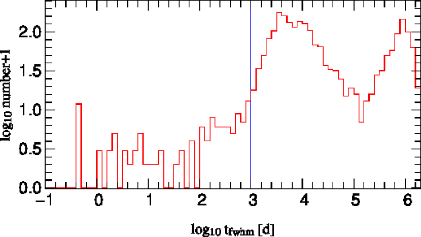
Figure 8: $t_{\mathrm{FWHM}}$ distrubtions of the 2247 detections passing criterion IV. The blue vertical line indicates the 1000 days upper limit in our selection criterion.

We note that the long timescale fits may arise from slowly moving objects. To test for this we inspect the positions of all detections passing criterion IV with $t_{\mathrm{FWHM}}$ $>$ 1000 days. We find that they are homogeneously distributed (they appear in some spikes of bright stars) except a small region close to a bright high proper motion object. This object influences the difference imaging kernel and therefore mimicking a proper motion of all other sources.

To demonstrate that 1000-d is a reasonable limit for $t_{\mathrm{FWHM}}$, we plot the $t_{\mathrm{FWHM}}$ and $\chi^{2}$ distributions of the events in Fig. 9. The yellow points are all detections passing criterion IV and with $t_{\mathrm{FWHM}}\geq$ 1000d. The green points are all detections passing criterion IV and with $t_{\mathrm{FWHM}}<$ 1000d. The magenta points are variables from Fliri et al. (2006). The blue points are novae from Lee et al. (2012). The red points with black dot are the 12 microlensing events presented in this paper.

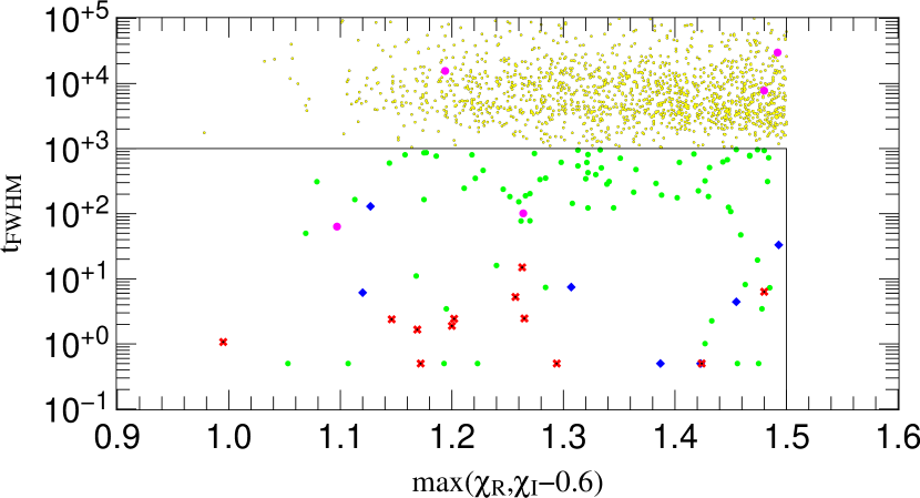
Figure 9: The events passing criterion IV, as well as our selection criteria of $t_{\mathrm{FWHM}}$ and $\chi^{2}$. The yellow points are all detections passing criterion IV and with $t_{\mathrm{FWHM}}\geq$ 1000d. The green points are all detections passing criterion IV and with $t_{\mathrm{FWHM}}<$ 1000d. The magenta points are variables from Fliri et al. (2006). The blue points are novae from Lee et al. (2012). The red points with black dot are the 12 microlensing events presented in this paper.

5 WeCAPP M31 lensing events

In this section we present the 12 microlensing events found in the WeCAPP data. Table 4 gives an overview on the properties of these 12 events. In this table we focus on two observables $t_{\mathrm{FWHM}}$ and ${\Delta_{F}}$. We fit the light curves with equation 2.

As shown in Table 4, the Paczynski-fit provides additional information on the Einstein timescale $t_{E}$ and the impact parameter $u_{0}$.

We note that the parameters $t_{\mathrm{FWHM}}$ and ${\Delta_{F}}$ are degenerate, which often leads to overestimated errors in these two parameters for very short time-scale events ($t_{\mathrm{FWHM}}$ below 2 day). Irrespective of this degeneracy, we can still determine these two parameters with reasonable uncertainty. To demonstrate the degeneracy, and our confidence in determining these two parameters, we show the 1, 2, and 3-$\sigma$ contour plot of $t_{\mathrm{FWHM}}$ vs. ${\Delta_{F}}$ in the appendix.

	RA(J2000)	Dec(J2000)	$\Delta_{\mathrm{M31}}$	$t_{0}$	$t_{\mathrm{FWHM}}$	$m_{R}$	${\Delta_{F}}_{R}$	$m_{I}$	${\Delta_{F}}_{I}$	(R-I)	log($t_{E}$)	log($u_{0}$)	$\chi^{2}_{dof}$
			[arcmin]	MJD [day]	[day]	[mag]	[$10^{-5}$ Jy]	[mag]	[$10^{-5}$ Jy]	[mag]	[day]	[$\theta_{E}$]
WeCAPP-01${\ddagger}$	00:42:30.03	41:13:01.5	4.08	$1850.84_{-0.02}^{+0.02}$	$1.62_{-0.10}^{+0.10}$	18.68	$10.29_{-0.53}^{+0.54}$	17.81	$18.22_{-0.98}^{+0.99}$	$0.88_{-0.03}^{+0.03}$	$7.85_{-0.01}^{+0.01}$	$-8.18_{-0.02}^{+0.02}$	1.21
WeCAPP-02	00:42:33.01	41:19:58.5	4.36	$1895.41_{-0.62}^{+0.71}$	$5.85_{-2.55}^{+3.04}$	20.81	$1.45_{-0.27}^{+0.37}$	19.64	$3.38_{-0.66}^{+0.88}$	$1.17_{-0.09}^{+0.09}$	$1.61_{-0.35}^{+0.29}$	$-1.36_{-0.49}^{+0.55}$	1.20
WeCAPP-03	00:42:57.03	41:12:27.9	4.40	$1585.35_{-0.18}^{+0.14}$	$2.44_{-0.26}^{+0.29}$	20.47	$1.99_{-0.04}^{+0.10}$	19.11	$5.51_{-0.11}^{+0.26}$	$1.36_{-0.04}^{+0.04}$	$2.64_{-0.62}^{+0.62}$	$-2.79_{-0.62}^{+0.62}$	1.23
WeCAPP-04	00:42:54.07	41:14:37.0	2.48	$2178.86_{-0.06}^{+0.06}$	$3.40_{-0.27}^{+0.27}$	20.18	$2.59_{-0.10}^{+0.10}$	19.58	$3.56_{-0.16}^{+0.16}$	$0.60_{-0.05}^{+0.05}$	$0.99_{-0.11}^{+0.11}$	$-0.93_{-0.15}^{+0.15}$	1.40
WeCAPP-05	00:43:02.03	41:18:29.2	4.09	$2177.85_{-0.40}^{+0.39}$	$6.34_{-1.10}^{+1.06}$	20.94	$1.29_{-0.09}^{+0.12}$	20.38	$1.71_{-0.16}^{+0.20}$	$0.56_{-0.11}^{+0.11}$	$1.47_{-0.32}^{+0.33}$	$-1.18_{-0.42}^{+0.39}$	1.38
WeCAPP-06	00:42:49.01	41:14:55.3	1.52	$2317.23_{-0.03}^{+0.03}$	$0.43_{-0.13}^{+0.16}$	18.15	$16.79_{-5.56}^{+4.47}$	17.36	$27.50_{-9.77}^{+7.84}$	$0.79_{-0.04}^{+0.03}$	$8.27_{-0.02}^{+0.02}$	$-9.18_{-0.11}^{+0.14}$	1.67
WeCAPP-07	00:42:55.03	41:18:50.9	3.38	$1847.44_{-0.15}^{+0.14}$	$1.24_{-0.34}^{+0.26}$	20.47	$1.99_{-0.30}^{+0.37}$	19.74	$3.08_{-0.43}^{+0.59}$	$0.73_{-0.13}^{+0.13}$	$8.68_{-0.07}^{+0.06}$	$-9.13_{-0.06}^{+0.05}$	1.02
WeCAPP-08	00:42:50.03	41:18:40.6	2.75	$2111.55_{-0.06}^{+0.10}$	$0.58_{-0.14}^{+0.16}$	19.11	$6.93_{-0.94}^{+0.87}$	18.36	$10.97_{-1.88}^{+1.59}$	$0.75_{-0.07}^{+0.06}$	$1.01_{-0.31}^{+0.27}$	$-1.77_{-0.38}^{+0.39}$	1.17
WeCAPP-09	00:42:44.07	41:12:54.9	3.22	$2231.67_{-0.41}^{+0.40}$	$14.04_{-1.38}^{+1.38}$	21.17	$1.05_{-0.05}^{+0.05}$	20.48	$1.55_{-0.10}^{+0.11}$	$0.68_{-0.07}^{+0.07}$	$1.53_{-0.15}^{+0.14}$	$-0.86_{-0.20}^{+0.20}$	1.42
WeCAPP-10	00:42:12.01	41:09:21.5	9.07	$4026.88_{-0.13}^{+0.13}$	$2.75_{-0.48}^{+0.42}$	21.01	$1.20_{-0.09}^{+0.12}$	20.10	$2.21_{-0.22}^{+0.26}$	$0.92_{-0.11}^{+0.11}$	$0.81_{-0.28}^{+0.33}$	$-0.83_{-0.46}^{+0.39}$	1.38
WeCAPP-11	00:42:46.02	41:15:11.9	1.01	$1198.81_{-0.18}^{+0.18}$	$6.41_{-0.79}^{+0.70}$	21.09	$1.13_{-0.07}^{+0.08}$	19.89	$2.69_{-0.16}^{+0.19}$	$1.20_{-0.08}^{+0.08}$	$1.21_{-0.36}^{+0.47}$	$-0.88_{-0.58}^{+0.43}$	1.62
WeCAPP-12	00:43:07.08	41:17:40.7	4.64	$4018.87_{-0.21}^{+0.24}$	$4.92_{-1.20}^{+1.08}$	20.64	$1.69_{-0.25}^{+0.30}$	19.80	$2.90_{-0.43}^{+0.53}$	$0.84_{-0.12}^{+0.12}$	$1.02_{-0.23}^{+0.25}$	$-0.79_{-0.41}^{+0.36}$	1.17

Table 4: Paczynski parameters of the WeCAPP microlensing events. In the fourth column we also show the distance from the M31 center. ^‡To determine the parameters of the light curve, we include data from POINT-AGAPE, as in Riffeser et al. (2003).

The light curves of the 12 WeCAPP events are shown in Figs 10-12. To illustrate the microlensing nature we also present postage stamps from the difference images close to the light curve maximum. These images help to rule out artifacts overseen by the pipeline, like hot pixels or cosmic rays as origin for the events. Indeed, as the inspection of the postage stamps show, none of our events is due to such an overseen artifact. In some cases (W2, W5, W7) the postage stamps also show positions of nearby variables. Because of improved photometric methods (see Riffeser et al., 2006), the light curves for W1 and W2 slightly differ from the published ones in Riffeser et al. (2003), but agree within the error bars.

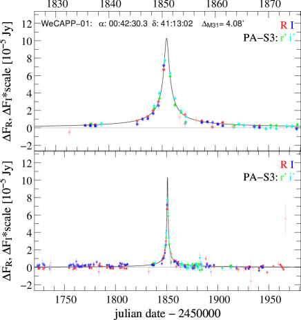
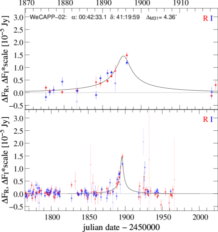
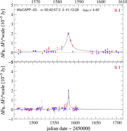
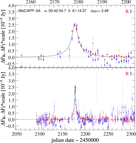
Figure 10: WeCAPP microlensing event light curves: WeCAPP 1-4 with corresponding cut-outs of the difference frames in R and I band. The data points are color-coded in grey-scale according to their errors; measurements with larger errors in R (I) are shown in light-red (light-blue), while measurements with smaller errors are shown in dark-red (dark-blue).

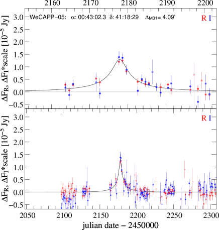
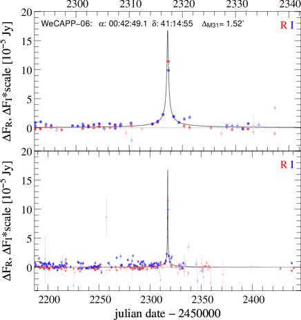
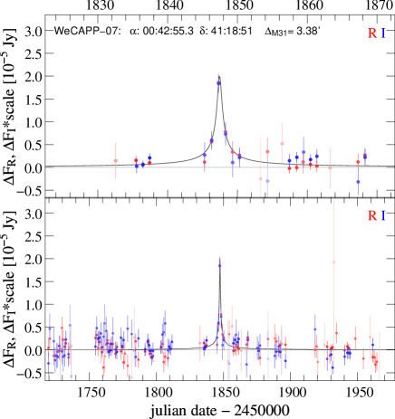
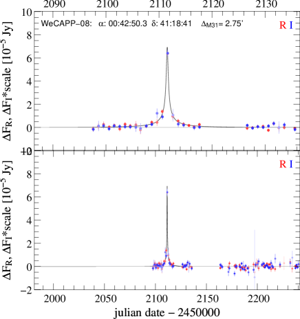
Figure 11: WeCAPP microlensing event light curves: WeCAPP 5-8 with corresponding cut-outs of the difference frames in R and I band.

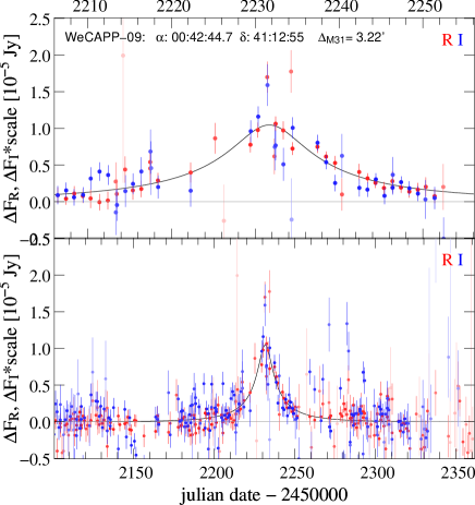
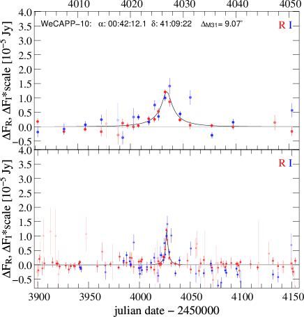
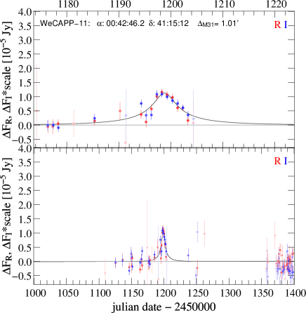
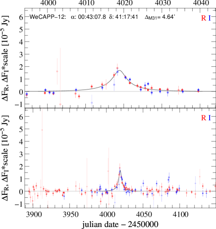
Figure 12: WeCAPP microlensing event light curves: WeCAPP 9-12 with corresponding cut-outs of the difference frames in R and I band.

6 Discussion

project	events	multi.	label in		recent
		detect.	Fig 13,14		citation
VATT/Columbia	6		VC	violet	Crotts & Tomaney (1996)
AGAPE	1		Z	gray	Ansari et al. (1999)
POINT-AGAPE	1		N1	blue	Aurière et al. (2001)
POINT-AGAPE	1		S4	blue	Paulin-Henriksson et al. (2002)
POINT-AGAPE	2	2	N, S	blue	Paulin-Henriksson et al. (2003)
WeCAPP	1	1	W	red	Riffeser et al. (2003)
POINT-AGAPE (MDM)	3		C	brown	Calchi Novati et al. (2003)
VATT/Columbia	4		VC	black	Uglesich et al. (2004)
MEGA	8	2	ML	green	de Jong et al. (2004)
POINT-AGAPE		1	N2	blue	An et al. (2004)
POINT-AGAPE	3	4	N, S	blue	Calchi Novati et al. (2005)
POINT-AGAPE	4	2	L1, L2	cyan	Belokurov et al. (2005)
Nainital	1		NMS	magenta	Joshi et al. (2005)
MEGA		5	ML	green	Cseresnjes et al. (2005)
MEGA	3	11	ML	green	de Jong et al. (2006)
WeCAPP		1	W	red	Riffeser et al. (2008)
PLAN	2		OAB	yellow	Calchi Novati et al. (2009)
PLAN		1	OAB	yellow	Calchi Novati et al. (2010)
PAndromeda	6		PAnd	orange	Lee et al. (2012)
PLAN		3	OAB	yellow	Calchi Novati et al. (2014)
WeCAPP	10	2	W	red	this work
total	56

Table 5: Overview of the 56 microlensing events in M31 presented in different papers. In the 3rd column for the total number we counted re-published detection only once. For comparison see Figure 14.

In this section we summarize M31 microlensing events from previous surveys we are aware of and we compare our 12 events with previous studies.

Table 5 lists the project name, number of detected events, their label and color as used in Figures 13 and 14, and the references for the events. In the 2^nd column we report the number of events that were solely detected by the corresponding survey. In the 3^rd column we list the number of events that were detected by more than one groups. For example, Paulin-Henriksson et al. (2003) published 4 events from the POINT-AGAPE project, where 2 of them were only detected by POINT-AGAPE, and 2 of them were also detected by other projects. Altogether 56 different M31 microlensing events have been published to date (including those presented in this work). Their $t_{0}$, $t_{\mathrm{FWHM}}$, ${\Delta_{F}}$ distributions are shown in Fig. 13. In Fig. 14 we show the positions of microlensing events in a 50$\times$70 arcmin² field from the 2^nd Palomar Sky Survey.

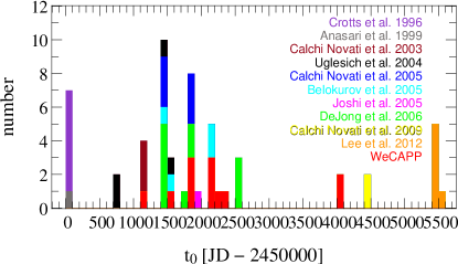
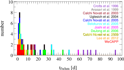
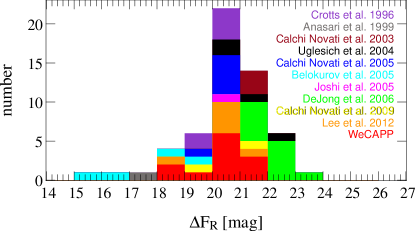
Figure 13: $t_{0}$, $t_{\mathrm{FWHM}}$ and ${\Delta_{F}}_{R}$ distribution of all microlensing events in M31 reported up to now. Short events seem to be frequent. Around 20 days there is a gap which separates short from long lensing events. The WeCAPP events are plotted in red, VATT/Columbia from Crotts & Tomaney (1996) in violet, POINT-AGAPE in blue, Belokurov-AGAPE in cyan, MEGA in green, AGAPE Z1 in gray, NMS in magenta, PLAN in yellow, SLOTT-AGAPE in brown, VATT/Columbia from Uglesich et al. (2004) in black, PAndromeda in orange. Note that the above distributions can not be directly taken to study the nature of events (halo vs. self-lensing) and to constrain the halo MACHO fraction, but instead have to be corrected for the surveys’ detection efficiencies.

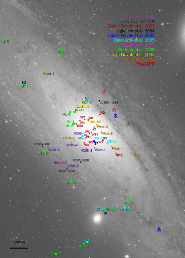
Figure 14: 56 microlensing events in M31. The image shows a wide field ($50\times 70$ arcmin) from the $2^{nd}$ Palomar Sky Survey (ESO Online Digitized Sky Survey - DSS-2-blue). The WeCAPP events are plotted in red, POINT-AGAPE events in blue, Belokurov events in cyan, MEGA events in green, AGAPE Z1 event in black, NMS event in magenta, PLAN events in yellow, PAndromeda events in orange, Slott-AGAPE in brown, VATT from Crotts & Tomaney (1996) in violet, and VATT from Uglesich et al. (2004) in black. We note that although our event W8 appears to be on top of the OAB-N2 event in this figure, their $t_{0}$ differ by more than 6.5 years (W8 has a $t_{0}$ of JD=2452112 and OAB-N2 has a $t_{0}$ of JD=2454467). In addition, from our difference images their positions differ by 0.5 arcsec.

The first fact to note in the middle panel of Fig. 13 is that WeCAPP (red), POINT-AGAPE (blue), and PLAN (yellow) surveys detected very short timescale events and hardly any events with $t_{\mathrm{FWHM}}>$ 15 days. In contrast, the first events ever announced by VATT/Columbia (Crotts & Tomaney, 1996, marked in violet color in Fig. 13) have very long timescales (5 of 6 events have $t_{\mathrm{FWHM}}>$ 65 days). In the same paper Crotts & Tomaney (1996) suspected that part of their events may be caused by long period variables. The MEGA (green) and Belokurov L2 (cyan) events show an almost flat timescale distribution. Five of the MEGA events are (in de-projection) located in the disk, almost at the same distance with respect to the M31 center. This makes them more suspicious, since they could be intrinsic varying disk stars that exist in a particular evolutionary time scale, that is overrepresented at this particular radius within the disk.

Predicting event rates and their characteristics from the theoretical studies, Riffeser et al. (2008) from their M31 microlensing model show the expected event rate of long timescale events ($t_{\mathrm{FWHM}}>$ 30 days) is an order of magnitude smaller than the event rate of short timescale events ($t_{\mathrm{FWHM}}<$ 10 days), see e.g. their Fig. 12. The fact that the vast majority of the events presented in this paper are short timescale events is therefore in good agreement with expectations. In contrast, VATT/Columbin and MEGA surveys show an almost flat timescale distribution. Unless surveys analyzed by MEGA and Belokurov et al. (2005) have detection efficiencies that strongly suppress events with timescales $<$ 10 days, they should have detected more short timescale microlensing. An alternative and more plausible explanation is that a large fraction of these long events are indeed long period variables, but were not ruled out from the microlensing candidate light curves due to the relative short time-span of the survey.

The VATT/Columbia team uses their observations in the 1994-1995 season to rule out objects of masses in the range of 0.003-0.08$M_{\odot}$ as the primary constituents of the mass of M31 (Crotts & Tomaney, 1996). Uglesich et al. (2004) find 4 probable microlensing events with data collected between 1997 and 1999. They conclude that 29${}^{+30}_{-13}$% of the halo masses are composed by MACHOs assuming a nearly singular isothermal sphere model. They also provide a poorly constrained lensing component mass (0.02-1.5 $M_{\odot}$ at 1$\sigma$ limits).

Calchi Novati et al. (2005) present an analysis of the POINT-AGAPE data. They indicate that their microlensing event rate is much larger than self-lensing expectation alone. This leads to a lower limit of 20% of the halo mass in the form of MACHOs with mass between 0.5-1 $M_{\odot}$ at the 95% confidence level. The lower limit drops to 8% for MACHOs $\sim$ 0.01 $M_{\odot}$.

On the contrary, the MEGA team (de Jong et al., 2006) conclude that their 14 events are consistent with self-lensing prediction. This rules out a MACHO halo fraction larger than 30% at the 95% confidence level. However, recent studies by Ingrosso et al. (2006, 2007) show that, when compared with the timescales, maximum fluxes, and spatial distributions from Monte-Carlo simulations, the MEGA events cannot be fully explained by self-lensing alone.

The evidence for MACHOs can be inferred from individual events provided good sampling of the light curves. For example, the WeCAPP-GL1/POINT-AGAPE-S3 event was independently discovered by the POINT-AGAPE (Paulin-Henriksson et al., 2003) and the WeCAPP (Riffeser et al., 2003) collaboration. Joint analysis of the light curves from these two collaborations has led to the conclusion that this event is very unlikely to be a self-lensing event (Riffeser et al., 2008). This is because with a realistic model of the three-dimensional light distribution, stellar population and extinction of M31, an self-lensing event with the parameters of WeCAPP-GL1/POINT-AGAPE-S3 is only expected to occur every 49 years. In contrast, a halo lensing event (with 20% of the M31 halo consists of 1 M_⊙ MACHOs) would occur every 10 years. In addition, combining the data from PLAN and WeCAPP, Calchi Novati et al. (2010) have revealed the finite-source effect in the event OAB-N2. Calchi Novati et al. (2010) then used the finite-source effect to determine the size of the Einstein ring radius, and combined the Einstein ring radius with the time required for the lens to travel the Einstein ring radius ($t_{\mathrm{E}}$) to derive the lens proper motion. Hence they were able to put a strong lower limit on the lens proper motion. Since the lens proper motion in the halo lensing scenario is different (and much larger) than the self-lensing scenario (see e.g. Fig. 4 of Calchi Novati et al., 2010), their result thus favors the MACHO lensing scenario over self-lensing for this event.

To conclude, some statistical studies and individual microlensing events point to a non-negligible MACHO population, though the fraction in the halo mass remains uncertain. To pinpoint the MACHO mass fraction, a better understanding of the luminous population, i.e. self-lensing rate, is needed.

Determining the MACHO mass fraction requires precise detection efficiency studies which is beyond the scope of this publication. We have started such efficiency studies (Koppenhoefer et al., in preparation). By simulating artificial events into the WeCAPP images we will be able to account for true noise and systematics introduced by the processing and the detection procedure. The results will enable us to derive a robust estimate of the MACHO mass fraction using an improved M31 model for disk, bulge and halo.

7 Summary and Outlook

WeCAPP has monitored the bulge of M31 for 11 years, which is the longest time-span among M31 microlensing surveys. We have established an automated selection pipeline and present the final 12 microlensing events from WeCAPP. The brightest event of it (see e.g. Riffeser et al., 2008) is hard to reconcile with self-lensing alone, hence hints at the existence of MACHOs in the halo of M31. A similar case has been found by Calchi Novati et al. (2010).

To gain insights to the MACHO fraction, in-depth understanding of self-lensing is required, which is only possible with microlensing experiments that monitor both the bulge and the disk of M31 simultaneously. With the advent of Pan-STARRS 1, we have conducted a dedicated project monitoring M31 with a field-of-view of $\sim$ 7 degree². Preliminary results of six microlensing events in the bulge have been published in Lee et al. (2012), and a full analysis will follow soon (Seitz et al. in prep.).

8 Acknowledgments

We are grateful to the referee for the very useful comments. We would like to thank Juergen Fliri, Christoph Ries, Otto Baernbantner, Claus Goessl, Jan Snigula and Sarah Buehler for their contributions in observation. This work was supported by the DFG cluster of excellence ’Origin and Structure of the Universe’ (www.universe-cluster.de).

9 Appendix

We show the degenercy between $t_{\mathrm{FWHM}}$ and ${\Delta_{F}}$ for our 12 WeCAPP microlensing events in Fig. 15. These two parameters are highly degenerate for very short time-scale events ($t_{\mathrm{FWHM}}$ below 2 day). For events with long time-scale, i.e. W3, W4, W5, W9, W10 and W11, their $t_{\mathrm{FWHM}}$ and ${\Delta_{F}}$ are well constrained.

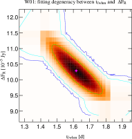
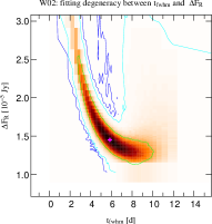
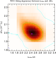
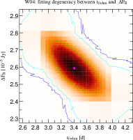
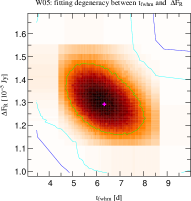
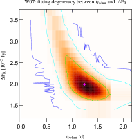
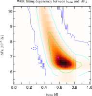
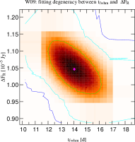
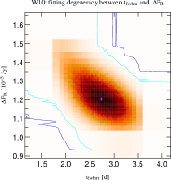
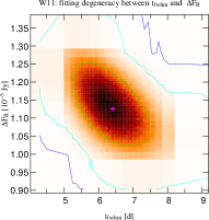
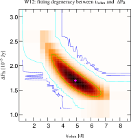
Figure 15: $t_{\mathrm{FWHM}}$ vs. ${\Delta_{F}}_{R}$ distribution of the 12 WeCAPP microlensing events. We note that the $t_{\mathrm{FWHM}}$ and ${\Delta_{F}}_{R}$-scale in the figures are different for each event. The 1, 2, and 3-$\sigma$ contours are marked in green, cyan and blue, respectively. The best-fit parameter is marked in magenta.

We also show the degeneracy between $t_{\mathrm{E}}$ and $u_{0}$ for our 12 WeCAPP microlensing events in Fig. 16. In the pixel-lensing regime, $t_{\mathrm{E}}$ and $u_{0}$ are highly degenerate, hence the $t_{\mathrm{E}}$-$u_{0}$ maps are much more degenerate than the $t_{\mathrm{FWHM}}$-${\Delta_{F}}$ maps.

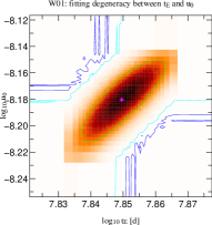
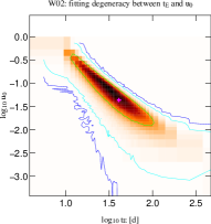
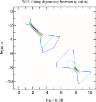
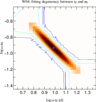
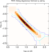
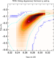
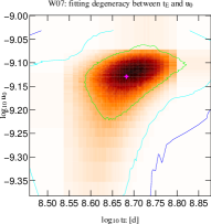
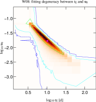
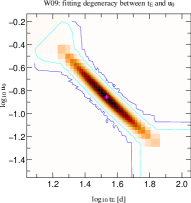
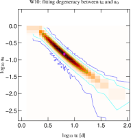
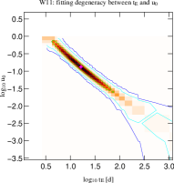
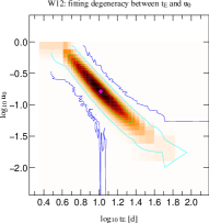
Figure 16: $t_{\mathrm{E}}$ vs. $u_{0}$ distribution in log scale of the 12 WeCAPP microlensing events. We note that the $t_{\mathrm{E}}$ and $u_{0}$-scale in the figures are different for each event. The 1, 2, and 3-$\sigma$ contours are marked in green, cyan and blue, respectively. The best-fit parameter is marked in magenta.

References

- Alard & Lupton (1998) Alard, C., & Lupton, R. H. 1998, ApJ, 503, 325
- Alcock et al. (1993) Alcock, C., Akerlof, C. W., Allsman, R. A., et al. 1993, Nature, 365, 621
- Alcock et al. (2000) Alcock, C., Allsman, R. A., Alves, D. R., et al. 2000, ApJ, 542, 281
- An et al. (2004) An, J. H., Evans, N. W., Kerins, E., et al. 2004, ApJ, 601, 845
- Ansari et al. (1997) Ansari, R., Auriere, M., Baillon, P., et al. 1997, A&A, 324, 843
- Ansari et al. (1999) Ansari, R., Aurière, M., Baillon, P., et al. 1999, A&A, 344, L49
- Aubourg et al. (1993) Aubourg, E., Bareyre, P., Bréhin, S., et al. 1993, Nature, 365, 623
- Aurière et al. (2001) Aurière, M., Baillon, P., Bouquet, A., et al. 2001, ApJ, 553, L137
- Baillon et al. (1993) Baillon, P., Bouquet, A., Giraud-Heraud, Y., & Kaplan, J. 1993, A&A, 277, 1
- Belokurov et al. (2005) Belokurov, V., An, J., Evans, N. W., et al. 2005, MNRAS, 357, 17
- Bennett (2005) Bennett, D. P. 2005, ApJ, 633, 906
- Besla et al. (2013) Besla, G., Hernquist, L., & Loeb, A. 2013, MNRAS, 428, 2342
- Calchi Novati et al. (2003) Calchi Novati, S., Jetzer, P., Scarpetta, G., et al. 2003, A&A, 405, 851