Thermofield-based chain mapping approach for open quantum systems

Abstract

We consider a thermofield approach to analyze the evolution of an open quantum system coupled to an environment at finite temperature. In this approach, the finite temperature environment is exactly mapped onto two virtual environments at zero temperature. These two environments are then unitarily transformed into two different chains of oscillators, leading to a one dimensional structure that can be numerically studied using tensor network techniques.

In the past decades, many different techniques have been developed to analyze the dynamics of quantum systems coupled to an environment, i.e. open quantum systems (OQS). Some of these are based on deriving a master equation, which evolves the reduced density operator of the OQS by tracing out the environment degrees of freedom breuerbook ; rivas2011a , and some others are based on the stochastic Schrödinger equations (SSE), evolving the OQS’s wave function conditioned by a continuous diosi1998 ; alonso2005 or discrete plenio1998 ; piilo2009 stochastic process. Both approaches are suitable for weak system-environment couplings, which generally lead to a large separation between system and environment time scales. Although such a large separation often occurs in quantum optics, it is not necessarily so in other scenarios, such as soft or condensed matter systems, or in quantum biology. In these situations, other approaches are more appropriate, such as the path integral Montecarlo wallsbook , which in some parameter regimes is nevertheless hindered by the sign problem, potentially affecting the convergence of the method at relatively short times (see for instance muelbacher2005 ).

An alternative is to solve the total system dynamics with exact diagonalization methods, which is difficult due to the large number of degrees of freedom in the environment. Hence, a wise selection of the relevant states of the full system is of primary importance, and this can be done for instance by discarding states with low probability, as in the density matrix approach zhang1998b (closely related to density matrix renormalization group), or by considering as relevant only those states generated during the evolution, as done in the variational approach bonca1999 ; vidmar2010 .

Similarly, it is possible to perform a unitary transformation of the environment that maps it onto a one dimensional structure. The numerical renormalization group (NRG) approach wilson1975 ; vojta2005 ; bulla2008 ; anders2007 ; weichselbaum2007 ; hughes2009 , for instance, is based on a (logarithmic) coarse-graining of the continuous environment spectral function in energy space. The resulting discretized environment can then be mapped onto a semi-infinite tight-binding chain krishna1980 with exponentially decreasing couplings. As proposed in prior2010 ; chin2010b ; chinbook2011 , the mapping can also be performed analytically without a previous discretization of the environment. Even when the couplings do not decay exponentially, it is typically possible to describe the system dynamics until its decay or relaxation time using a truncated chain of finite length. The total system can now be modelled as a matrix product state (MPS), and it is then possible to use tensor network techniques to simulate the unitary evolution of the total system vidal2003 ; verstraete08algo ; scholl2011 ; scholl2005 . The approach can also deal with an environment at finite temperature, using matrix product operators verstraete2004 ; zwolak2004 .

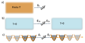
Figure 1: Fig. a) represents the initial problem described with (1) of an OQS coupled to a harmonic oscillator reservoir at finite temperature. Fig. b) represents the thermofield-transformed problem (2), in which the finite temperature of the reservoir is encoded in two different reservoirs at zero temperature. Fig. c) is the chain representation of the latter.

In this letter we present a complementary formulation of this idea based on the thermofield approach proposed in bargmann1961 ; araki1963 ; takahashi1975 (see blasonebook for a review). In this approach, the environmental Hilbert space is mirrored or doubled, and then a thermal Bogoliubov transformation is performed. As a result, the real environment in a thermal state is transformed into two virtual environments in a vacuum state (see Fig. 1.b), known in the literature as the thermofield vacuum. The expectation value of any operator of the real environment in the thermofield vacuum coincides with its expectation value in the thermal state. The only excitations appearing in the environment will be those that are dynamically created through the interaction, and the dynamics of the resulting transformed system can be simulated using MPS.

The thermofield approach has been considered in the framework of SSE of OQS (see for instance diosi1998 ), but most of its applications are in the context of quantum field theory and general relativity maldacena2013 ; israel1976 .

Thermofield dynamics– Let us consider an environment of harmonic oscillators, with annihilation (creation) operators $b_{k}$ ($b_{k}^{\dagger}$) and frequencies $\omega_{k}$, to which the OQS couples with strengths $g_{k}$. The complete Hamiltonian can be written as

$$H_{\textmd{tot}}=H_{S}+\sum_{k}\omega_{k}b^{\dagger}_{k}b_{k}+\sum_{k}g_{k}(L^{\dagger}b_{k}+b_{k}^{\dagger}L),$$ (1)

where $H_{S}$ is the Hamiltonian of the OQS, and $L$ is the coupling operator acting on the OQS Hilbert space. We can introduce an auxiliary, decoupled environment, characterized by annihilation (creation) operators $c_{k}$ ($c_{k}^{\dagger}$) and write the total Hamiltonian as

$$\hat{H}_{\textmd{tot}} = H_{\textmd{tot}}-\sum_{k}\omega_{k}c^{\dagger}_{k}c_{k}.$$ (2)

Assuming now that both environments are initially in a thermal state at inverse temperature $\beta$, we apply a thermal Bogoliubov transformation,

$$a_{1k} = e^{-iG}b_{k}e^{iG}=\cosh(\theta_{k})b_{k}-\sinh(\theta_{k})c^{\dagger}_{k},$$ (3)

$$a_{2k} = e^{-iG}c_{k}e^{iG}=\cosh(\theta_{k})c_{k}-\sinh(\theta_{k})b^{\dagger}_{k}.$$ (4)

Here, $G=i\sum_{k}\theta_{k}(b_{k}^{\dagger}c^{\dagger}_{k}-c_{k}b_{k})$, with $\theta_{k}$ a function of the temperature such that $\cosh(\theta_{k})=\sqrt{1+n_{k}}$, and $n_{k}=1/(e^{\beta\omega_{k}}-1)$ is the number of excitations in mode $k$. In terms of these new modes,

$$\hat{H}_{\textmd{tot}}=H_{S}+\sum_{k}\omega_{k}\large(a_{1k}^{\dagger}a_{1k}-a^{\dagger}_{2k}a_{2k}\large)$$ (5)

$$+ \sum_{k}g_{1k}(L^{\dagger}a_{1k}+a^{\dagger}_{1k}L)+\sum_{k}g_{2k}(La_{2k}+a^{\dagger}_{2k}L^{\dagger}),$$ (6)

where, $g_{1k}=g_{k}\cosh(\theta_{k})$ and $g_{2k}=g_{k}\sinh(\theta_{k})$. The thermal vacuum can be written in terms of the vacuum for $b_{k}$, $c_{k}$ modes, $|\Omega_{0}\rangle$, as

$$|\Omega\rangle=e^{-iG}|\Omega_{0}\rangle.$$ (7)

The thermal vacuum can be written in alternative ways that further enlighten its physical meaning. Firstly, it can be written as $|\Omega\rangle=e^{-S/2}e^{\sum_{k}b_{k}^{\dagger}c_{k}^{\dagger}}|\Omega_{0}\rangle$, with $S=-\sum_{k}(b_{k}^{\dagger}b_{k}\log\sinh^{2}(\theta_{k})-b_{k}b_{k}^{\dagger}\log\cosh^{2}(\theta_{k}))$, which can be interpreted as the entropy operator for the physical (original) environment blasonebook , since the thermofield vacuum is the state that minimizes the thermodynamic potential $\langle\Omega|(-\frac{1}{\beta}S+H)|\Omega\rangle$. Secondly, up to normalization, $|\Omega\rangle\propto e^{-\beta H_{B}/2}|I\rangle$, where $|I\rangle=\sum_{n}|n\rangle_{b}|n\rangle_{c}$ is a maximally entangled state between the real and the auxiliary environments, defined in terms of their energy eigenstates, $|n\rangle_{b}$, $|n\rangle_{c}$. The thermal state of the original environment is thus $\rho_{B}=\textmd{Tr}_{\textmd{aux}}[|\Omega\rangle\langle\Omega|]$ and it can be approximated by a MPO by evolving the maximally entangled state in imaginary time verstraete2004 ; zwolak2004 . In contrast, the present approach is based on directly calculating the dynamics of the whole system under the Hamiltonian (6), using the thermofield vacuum as (pure) initial state for both reservoirs. Although this state is annihilated by $a_{1k}$ and $a_{2k}$, the number of physical particles has non-vanishing expectation value $n_{k}=\langle\Omega|b_{k}^{\dagger}b_{k}|\Omega\rangle=\sinh^{2}(\theta_{k})$. Hence, solving the dynamics of the initial problem (1) with an initial condition $\rho_{0}^{\textmd{tot}}=\rho^{S}_{0}\otimes\rho^{\textmd{th}}_{B}$, with $\rho_{0}^{S}$ the initial state of the system, is equivalent to solving the dynamics with (6), but considering $\rho_{0}^{\textmd{tot}}=\rho^{S}_{0}\otimes|\Omega\rangle\langle\Omega|$ (see Fig. (1a) and (1b) respectively). We have described in detail the thermofield transformation for bosonic environments, but a similar Bogoliubov transformation can be proposed for fermionic reservoirs. In that case blasonebook we have $a_{1k}=e^{-iG}b_{k}e^{iG}=\cos(\theta_{k})b_{k}-\sin(\theta_{k})c^{\dagger}_{k}$, and $a_{2k}=e^{-iG}c_{k}e^{iG}=\cos(\theta_{k})c_{k}+\sin(\theta_{k})b^{\dagger}_{k}$. With this transformation, the Hamiltonian (2) is transformed into (6).

Chain representation– The Hamiltonian (6) represents an OQS interacting with two independent environments, having operators $a_{1k}$ and $a_{2k}$ respectively. The whole problem can be mapped into a one dimensional structure with the schematic form in Fig. (1c). In general, the environment oscillators in (1) form a quasi-continuum, so that the Hamiltonian can also be written as $H=H_{S}+\int_{0}^{1}dkg(k)(b(k)L^{\dagger}+Lb(k)^{\dagger})+\int_{0}^{1}\omega(k)b(k)^{\dagger}b(k)$. When the environment is in a Gaussian state, $\omega(k)$ and $g(k)$ enter the description of the OQS only through the spectral density, $J(\omega)$. In this situation, one can always choose $\omega(k)=\omega_{0}k$ (with $\omega_{0}$ an arbitrary constant that may be taken as one), and $\hat{g}(k)=\sqrt{J(\omega(k))}$. Similarly, the continuum representation of (6) reads

$$\tilde{H}_{\textmd{tot}} =H_{S}+\int_{0}^{1}dkk\large(a_{1k}^{\dagger}a_{1k}-a^{\dagger}_{2k}a_{2k}\large)$$ (8)

$$+\int_{0}^{1}dk\large[\hat{g}_{1k}(L^{\dagger}a_{1k}+a^{\dagger}_{1k}L)+\hat{g}_{2k}(La_{2k}+a^{\dagger}_{2k}L^{\dagger})\large]$$

Thus, the spectral densities are $J_{1}(k)=\hat{g}_{1}^{2}(k)=\sum_{k}(1+n(\omega(k)))J(\omega(k))$, and $J_{2}(k)=\hat{g}_{2}^{2}(k)=n(\omega(k))J(\omega(k))$. Then, using the unitary transformation discussed in prior2010 ; chin2010b , new bosonic operators $B_{n}$ and $C_{n}$ can be defined for each reservoir, such that

$$a_{1k}=\sum_{n}U_{1n}(k)B_{n},\quad a_{2k}=\sum_{n}U_{2n}(k)C_{n},$$ (9)

where $U_{jn}(k)=g_{j}(k)\pi_{jn}(k)/\rho_{nj}$ ($j=1,2$). Here, $\pi_{jn}(k)$ are monic orthogonal polynomials that obey $\int_{0}^{1}dkJ_{j}(k)\pi_{j,n}(k)\pi_{j,m}(k)=\rho_{nj}^{2}\delta_{nm}$, with $\rho^{2}_{nj}=\int_{0}^{1}dkJ_{j}(k)\pi^{2}_{j,n}(k)$ chin2010b ; chinbook2011 . Hence, the proposed transformation is also orthogonal, $\int dkU^{*}_{jn}U_{jm}=\delta_{nm}$. The transformed Hamiltonian can be written as $H_{tot}=H_{S}+H_{B}+H_{\textmd{int}}$, with $H_{\textmd{int}}=g_{1}(L^{\dagger}B_{0}+B_{0}^{\dagger}L)+g_{2}(LC_{0}+C_{0}^{\dagger}L^{\dagger})$, with $g_{j}=\rho_{j0}$, and

$$H_{B}= \sum_{n=0,\cdots,M}(\alpha_{1,n}B_{n}^{\dagger}B_{n}-\alpha_{2,n}C_{n}^{\dagger}C_{n}$$

$$+ \sqrt{\beta_{1,n+1}}B^{\dagger}_{n+1}B_{n}-\sqrt{\beta_{2,n+1}}C^{\dagger}_{n+1}C_{n}+h.c.),$$ (10)

where the recurrence relation of the polynomials has been used, $\pi_{j,n+1}(k)=(k-\alpha_{j,n})\pi_{n}(k)-\beta_{j,n}\pi_{j,n-1}(k)$, with $\pi_{j,n-1}=0$. Coefficients $\alpha_{j,n}$ and $\beta_{j,n}$ can be obtained with standard numerical routines gautschi2005 . The resulting Hamiltonian describes two tight-binding chains to which the system is coupled. The thermofield vacuum is also annihilated by the new modes $B_{n}$ and $C_{n}$, so that the dynamics of the whole system can be simulated using MPS time-evolution methods from an initial state with zero occupancy of each of these modes.

A similar mapping can be applied in the case of a finite discrete environment by means of a standard tri-diagonalization.

In the following, we present numerical results to illustrate this approach in different examples.

Example 1: A spin in a bosonic field– Let us consider a spin $1/2$ system coupled to a bosonic environment with spectral density given by the Caldeira and Leggett model leggett1987 ; weissbook ,

$$J(\omega)=\eta\omega^{s}e^{-\omega/\omega_{c}},$$ (11)

with $0<s<1$ in the sub-ohmic case, and $s>1$ in the super-ohmic. Roughly speaking, the constant $\eta$ gives the coupling strength between system and environment. The exponential factor in (11) provides a smooth cut-off for the spectral density, modulated by a frequency cut-off $\omega_{c}$. This general model provides a good approximation for spectral densities appearing in many different problems, like an impurity in a photonic crystal florescu2001 ; devega2005 , quantum impurity models si2001 , and solid state devices at low temperatures such as superconducting qubits shnirman2002 , quantum dots tong2006 , and nanomechanical oscillators seoanez2007 , to name just a few examples. As a first check we consider a solvable example, with $H_{S}=\frac{1}{2}\hbar\omega_{S}\sigma_{z}$, and $L=\sigma_{z}$ in (1). For an initial state $|\psi_{0}\rangle=a|0\rangle+b|1\rangle$, the expectation value of any system operator, $A$, can be analytically calculated alonso2007 ,

$$\langle A(t)\rangle = e^{-2\phi_{t}}\big{\{}|a|^{2}e^{i\omega_{S}t}+|b|^{2}e^{-i\omega_{S}t}\big{\}},$$ (12)

with $\phi_{t}=\int_{0}^{t}d\tau\int_{0}^{\tau}ds\textmd{Re}[\alpha_{T}(\tau-s)]$, $\alpha_{T}(t)=\sum_{k}g_{k}^{2}\left[\coth{(\frac{\omega_{k}\beta}{2})}\cos{(\omega_{k}t)-i\sin{(\omega_{k}t)}}\right]$.

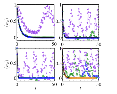
Figure 2: Evolution of the mean value of $\langle\sigma_{x}(t)\rangle$ for $a=b=1/\sqrt{2}$, for $\eta=0.1$ and $\omega_{S}=0$. Upper panels correspond to the ohmic model ($s=1$), for $\beta=5$ (left) and $\beta=1$ (right panel). The two lower panels correspond respectively to a sub-ohmic model with $s=1/2$ (left panel), and a super-ohmic model with $s=3/2$ (right panel), both for $\beta=1$. The exact solution is given by the solid black curves. For the MPS, we consider a varying $M$: magenta, green and blue curves correspond to $M=2,10,40$ respectively in all plots. The last plot includes an orange curve with $M=120$. Bond dimension is $D=20$, and maximum occupation numbers in the harmonic oscillator basis is $n=3$.

To simulate the problem numerically using MPS we need to truncate the maximum occupation number of the bosonic modes, and the length of the chains corresponding to the transformed environment. We compare the numerical solution to the exact one for $A=\sigma_{x}$ in Fig. 2. and observe very good agreement for all considered spectral densities, couplings and temperatures, for a relatively small bond dimension and length of each chain, $M$.

In the following, we consider a problem that is not exactly solvable, by choosing $L=\sigma_{x}$, and compare the solutions of our method with those corresponding to a master equation (ME) up to second order in the system-environment coupling parameter $g$

$$\frac{d\rho_{s}(t)}{dt} = -i[H_{S},\rho_{s}(t)]+\int_{0}^{t}d\tau\alpha_{2}^{*}(t-\tau)[L^{\dagger},\rho_{s}(t)L(\tau-t)]$$ (13)

$$+ \int_{0}^{t}d\tau\alpha_{2}(t-\tau)[L^{\dagger}(\tau-t)\rho_{s}(t),L]$$

$$+ \int_{0}^{t}d\tau\alpha_{1}(t-\tau)[L(\tau-t)\rho_{s}(t),L^{\dagger}]$$

$$+ \int_{0}^{t}d\tau\alpha_{1}^{*}(t-\tau)[L,\rho_{s}(t)L(\tau-t)^{\dagger}]+{\mathcal{O}}(g^{3}),$$

with $\alpha_{1}(t-\tau)=\sum_{k}g^{2}_{k}(n_{k}+1)e^{-i\omega_{k}(t-\tau)}$, $\alpha_{2}(t-\tau)=\sum_{\lambda}g^{2}_{k}n_{k}e^{i\omega_{k}(t-\tau)}$, and $L(t)=e^{iH_{S}t}Le^{-iH_{S}t}$.

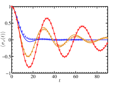
Figure 3: Comparison of ME (solid curves) with MPS (triangles) results for $\langle\sigma_{x}(t)\rangle$ considering $\eta=0.01$, $\omega_{S}=0.1$, and $M=100$ for both chains. We consider $\beta=10$ (blue), $\beta=50$ (orange) and $\beta=1000$ (red). The MPS results converge with maximum population per oscillator $n=4$.

To derive this equation, the Born approximation has also been assumed. This ME neglects the system-environment correlations, and considers that the latter remains in the thermal equilibrium state $\rho_{B}$ during the interaction, so that $\rho_{\textmd{tot}}(t)\approx\rho_{s}(t)\otimes\rho_{B}$.

As shown in Fig. (3), the ME and the MPS coincide quite reasonably at weak couplings. However, as shown in Fig. (4), for stronger couplings the ME does not give an accurate description of the dynamics. Indeed, the MPS results describe comparatively a much slower decay for the two temperature values here considered. Also, the computational cost of the MPS in the strong coupling regime is much higher than at weak coupling. Nevertheless, the difference of the present scheme is that the excitations involved in the numerical resolution are just those that are dynamically generated due to the interaction with the OQS. This is in clear contrast with traditional methods in which the initial state is thermal, and therefore already has a finite initial occupation in the environment basis.

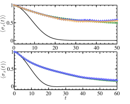
Figure 4: Evolution of $\langle\sigma_{x}(t)\rangle$ for $\beta=10$ (upper panel, with maximum bond dimension $D=40$) and $\beta=50$ (lower panel, with $D=20$) for $\eta=0.1$, $\omega_{S}=0.1$, and $M=100$ for both chains. The solid black curve corresponds to the solution for the ME. Considering $n_{1}$ the dimension of the first two oscillators in the chain, and $n_{2}$ the dimension of the following ones, the curves with green squares correspond to $(n_{1}=5,n_{2}=4)$, and the ones with blue diamonds to $(n_{1}=6,n_{2}=5)$ (lower panel) and $(n_{1}=7,n_{2}=6)$ (upper panel). The curve with orange triangles in the upper panel corresponds to $(n_{1}=8,n_{2}=7)$.

Example 2: A quantum dot coupled to an electronic reservoir– As noted above, our proposal is valid also for fermionic environments. To illustrate this, we consider a quantum dot (QD) coupled to an electronic reservoir at a finite temperature with a Hamiltonian $H=H_{S}+H_{\rm B}+H_{\rm hy}$. Here, $H_{S}=\sum_{\sigma}(Vn_{\sigma}+\frac{U}{2}~{}n_{\sigma}n_{\bar{\sigma}})$ is the Hamiltonian of the quantum dot, which is represented using the Anderson impurity model with an on-site Coulomb repulsion $U$ and an on-site energy $V$. Here, the operator $n_{\sigma}=d^{\dagger}_{\sigma}d_{\sigma}$ measures the number of electrons with spin $\sigma=\uparrow,\downarrow$ at the dot. We consider that the QD is connected to the reservoir through a hybridization term $H_{\rm hy}=-t\sum_{k;\sigma}g_{k}(d^{\dagger}_{\sigma}b_{k}+{\rm h.c.})$, that is a sum of bilinear terms wherein $d^{\dagger}_{i\sigma}$($d_{i\sigma}$) creates (annihilates) an electron at the dot with spin $\sigma$ and $b^{\dagger}_{k}$($b_{k}$) creates (annihilates) an electron with arbitrary spin and momentum $k$ in the reservoir. Hence, the interaction Hamiltonian has a similar form as the one in (1), but redefining $L=-t\sum_{\sigma}d_{\sigma}$. For simplicity, we have considered that both spins $\sigma$ couple equally to the reservoir. The Hamiltonian of the environment is $H_{\rm B}=\sum_{k}\omega_{k}b_{k}^{\dagger}b_{k}$. After the thermofield transformation, the former Hamiltonian is written in terms of $\tilde{H}_{\rm B}=\sum_{k}\omega_{k}(a_{1k}^{\dagger}a_{1k}-a_{2k}^{\dagger}a_{2k})$, and an interaction Hamiltonian of the form (6) with couplings $g_{1k}=-tg_{k}\sqrt{1+f_{k}}$, and $g_{2k}=-tg_{k}\sqrt{f_{k}}$, with $f_{k}=(1+\exp(\beta\omega_{k}))^{-1}$. We consider a spectral density of sub-ohmic type, with $s=0.5$ in Eq. (11).

Comparing the MPS results to those of ME, as shown in Fig. 5, we find initial agreement as expected, but then the results start to differ considerably even at relatively weak couplings. Due to the limited size of the fermionic basis, the MPS converges to the exact result with relatively small computational resources.

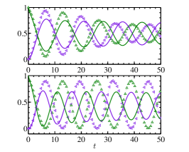
Figure 5: Evolution of $\langle n_{\uparrow}\rangle$ (green) and $\langle n_{\downarrow}\rangle$ (purple) for the ME (solid lines) and the t-DMRG (symbols). We have considered $\beta=1$ (upper panel), $\beta=10$ (lower panel) with $U=0.2$, $V=-U/2$, $\omega_{c}=15$, $t=0.01$, and a $M=100$ oscillators in the chain.

Conclusions and outlook– Based on a thermofield approach, our formalism allows us to efficiently integrate the dynamics of an OQS coupled to a thermal reservoir, either bosonic or fermionic, in a pure state formalism, without previously preparing the thermal state with imaginary time evolution. The approach is based on performing an analytical (thermal Bogoliubov) transformation over the (physical) environment and an auxiliary one. Provided the thermal state of the original environment is known, more concretely, that the quantities $n_{k}$ can be analytically or numerically computed, our approach can be used to solve thermalization problems of OQS using only zero-temperature (pure state) MPS.

Acknowledgment: We thank D. Alonso, U. Schollwöck, F. Heidrich-Meisner, and C.A. Büsser for helpful discussions. This work was supported by Nanosystems Initiative Munich (NIM) (project No. 862050-2), and partially by the Spanish MICINN (Grant No. FIS2013-41352-P), and the EU through SIQS grant (FP7 600645).

References

- (1) H. Breuer and F. Petruccione, The theory of Quantum Open Systems (Oxford Univ. Press, 2002).
- (2) A. Rivas and S. F. Huelga, Open Quantum Systems. An Introduction (Springer, Heidelberg) (2011).
- (3) L. Diósi, N. Gisin, and W. T. Strunz, Phys. Rev. A 58, 1699 (1998).
- (4) D. Alonso and I. de Vega, Phys. Rev. Lett. 94, 200403 (2005).
- (5) M. Plenio and P. Knight, Rev. Mod. Phys 70, 101 (1998).
- (6) J. Piilo, K. Härkönen, S. Maniscalco, and K.-A. Suominen, Phys. Rev. A 79, 062112 (2009).
- (7) D. Walls and G. Milburn, Quantum Optics (Springer Verlag, 1994).
- (8) L. Mühlbacher and J. Ankerhold, J. Chem. Phys. 122, 184715 (2005).
- (9) C. Zhang, E. Jeckelmann, and S. R. White, Phys. Rev. Lett. 80, 2661 (1998).
- (10) J. Bonča, S. A. Trugman, and I. Batistić, Phys. Rev. B 60, 1633 (1999).
- (11) L. Vidmar, J. Bonča, and S. A. Trugman, Phys. Rev. B 82, 104304 (2010).
- (12) K. G. Wilson, Rev. Mod. Phys. 47, 773 (1975).
- (13) M. Vojta, N.-H. Tong, and R. Bulla, Phys. Rev. Lett. 94, 070604 (2005).
- (14) R. Bulla, T. A. Costi, and T. Pruschke, Rev. Mod. Phys. 80, 395 (2008).
- (15) F. B. Anders, R. Bulla, and M. Vojta, Phys. Rev. Lett. 98, 210402 (2007).
- (16) A. Weichselbaum and J. von Delft, Phys. Rev. Lett. 99, 076402 (2007).
- (17) K. Hughes, C. Christ, and I. Burghardt, J. Chem. Phys 131, 024109 (2009).
- (18) H. R. Krishna-murthy, J. W. Wilkins, and K. G. Wilson, Phys. Rev. B 21, 1003 (1980).
- (19) J. Prior, A. W. Chin, S. F. Huelga, and M. B. Plenio, Phys. Rev. Lett. 105, 050404 (2010).
- (20) A. W. Chin, A. Rivas, S. F. Huelga, and M. B. Plenio, J. Math. Phys. 51,, 092109 (2010).
- (21) A. W. Chin, S. F. Huelga, and M. B. Plenio, in Semiconductors and Semimetals, edited by U. Wurfel, M. Thorwart, E. R. Weber, and C. Jagadish (Academic Press, 2011).
- (22) G. Vidal, Phys. Rev. Lett. 91, 147902 (2003).
- (23) F. Verstraete, V. Murg, and J. Cirac, Advances in Physics 57, 143 (2008).
- (24) U. Schollwöck, Ann. Phys. N.Y. 326, 96 (2011).
- (25) U. Schollwöck, Rev. Mod. Phys. 77, 259 (2005).
- (26) F. Verstraete, J. J. García-Ripoll, and J. I. Cirac, Phys. Rev. Lett. 93, 207204 (2004).
- (27) M. Zwolak and G. Vidal, Phys. Rev. Lett. 93, 207205 (2004).
- (28) V. Bargmann, Communications on Pure and Applied Mathematics 14, 187 (1961).
- (29) H. Araki and E. J. Woods, J. Math. Phys 4, 637 (1963).
- (30) H. U. Y. Takahashi, Collect. Phenom. 2, 55 (1975).
- (31) M. Blasone, P. Jizba, and G. Vitiello, Quantum Field Theory and Its Macroscopic Manifestations Boson Condensation, Ordered Patterns and Topological Defects (World Scientific Singapore, 2011).
- (32) J. Maldacena and L. Susskind, (2013).
- (33) W. Israel, Physics Letters A 57, 107 (1976).
- (34) W. Gautschi, Journal of Computational and Applied Mathematics 178, 215 (2005), proceedings of the Seventh International Symposium on Orthogonal Polynomials,Special Functions and Applications.
- (35) A. J. Leggett et al., Rev. Mod. Phys. 59, 1 (1987).
- (36) U. Weiss, in Quantum Dissipative Systems, edited by W. Scientific (Series in modern condensed matter systems, 2008).
- (37) M. Florescu and S. John, Phys. Rev. A 64, 033801 (2001).
- (38) I. de Vega, D. Alonso, and P. Gaspard, Phys. Rev. A 71, 023812 (2005).
- (39) Q. Si, S. Rabello, K. Ingersent, and J. L. Smith, Nature 413, 804 (2001).
- (40) A. Shnirman, Y. Makhlin, and G. Schön, Physica Scripta 2002, 147 (2002).
- (41) N.-H. Tong and M. Vojta, Phys. Rev. Lett. 97, 016802 (2006).
- (42) C. Seoanez, F. Guinea, and A. H. C. Neto, EPL (Europhysics Letters) 78, 60002 (2007).
- (43) D. Alonso and I. de Vega, Phys. Rev. A 75, 052108 (2007).