Infinite matrix product states, boundary conformal field theory, and the open Haldane-Shastry model

Abstract

We show that infinite Matrix Product States (MPS) constructed from conformal field theories can describe ground states of one-dimensional critical systems with open boundary conditions. To illustrate this, we consider a simple infinite MPS for a spin-1/2 chain and derive an inhomogeneous open Haldane-Shastry model. For the spin-1/2 open Haldane-Shastry model, we derive an exact expression for the two-point spin correlation function. We also provide an SU($n$) generalization of the open Haldane-Shastry model and determine its twisted Yangian generators responsible for the highly degenerate multiplets in the energy spectrum.

Introduction.— For a long time, it has been known that the main curse of quantum many-body theory is the exponential growth of the Hilbert space dimension with respect to the number of constituting particles. In the last decades, the study of entanglement has significantly alleviated this curse, at least to some extent, by recognizing the fact that only a tiny corner of the Hilbert space, with small amount of entanglement, is pertinent for the low-energy sector of Hamiltonians with local interactions. This deep insight lies at the heart of tensor network states Verstraete08 , a family of trial wave functions designed for efficiently representing the physically relevant states in the tiny corner. The best known instance among them is the Matrix Product States (MPS) in one spatial dimension, described in terms of local matrices with finite dimensions. Their entanglement entropies are bounded by the local matrix dimensions, which are nevertheless sufficient for accurately approximating gapped ground states of one-dimensional (1D) local Hamiltonians Verstraete06 ; Hastings07 . This discovery not only provides a transparent theoretical picture for real-space renormalization group methods Wilson75 ; White92 , but also leads to a recent complete classification of all possible 1D gapped phases Pollmann10 ; Chen11 ; Norbert2011 .

For 1D critical systems, the low-energy physics is usually described by conformal field theories (CFT). Their ground-state entanglement entropies exhibit unbounded logarithmic growth Holzhey04 ; Vidal03 ; Calabrese04 with respect to the subsystem size, indicating the deficiency of a usual MPS description. To overcome this difficulty, infinite MPS, whose local matrices are conformal fields living in an infinite-dimensional Hilbert space, have been introduced in Ref. Ignacio10 . The lattice sites for the infinite MPS locate on a unit circle, embedded in a complex plane. This construction shares conceptual similarity to Moore and Read’s approach Moore91 of writing 2D trial fractional quantum Hall states in terms of conformal blocks. For a variety of examples Ignacio10 ; Anne11 ; Tu13 ; Tu14a ; Tu14b ; Bondesan14 ; Ivan14 ; Benedikt15 , the infinite MPS (as well as their parent Hamiltonians) have been shown to describe critical chains with periodic boundary conditions (PBC) and, furthermore, their critical behaviors are often related to the CFT whose fields are used for constructing the wave functions exception . In this sense, the infinite MPS introduced in Ref. Ignacio10 provide a systematic way of finding lattice discretizations of CFT.

In this Rapid Communication, we show that the infinite MPS ansatz can describe ground states of 1D critical systems with open boundary conditions (OBC), thus complementing the PBC case in Ref. Ignacio10 . Unlike bulk CFT for periodic chains, open critical chains are instead described by boundary CFT. Taking a spin-1/2 chain as an example, we show how the infinite MPS with an image prescription allows us to derive an inhomogeneous open Haldane-Shastry model, including the original spin-1/2 open Haldane-Shastry models Simons94 ; Bernard95 as special cases. Within the new formalism, an exact expression for the two-point spin correlator of the spin-1/2 open Haldane-Shastry model is obtained. This, together with numerical results for the entanglement entropy, is in perfect agreement with the theoretical predictions based on boundary CFT, which thus confirms that our infinite MPS with the image prescription is suitable for describing open critical chains. The open infinite MPS construction is readily applicable to any boundary CFT for finding their lattice discretizations. As a further example, we derive an SU($n$) generalization of the open Haldane-Shastry model. We characterize its full spectrum and also determine the twisted Yangian generators responsible for the highly degenerate multiplets in the energy spectrum.

Infinite MPS and parent Hamiltonian.— Let us consider a spin-1/2 chain located on the upper unit circle in the complex plane, with $L$ lattice sites and complex lattice coordinates $z_{j}=e^{i\theta_{j}}$ ($j=1,\ldots,L$ and $\theta_{j}\in[0,\pi]$ $\forall j$), see Fig. 1(a). We denote by $S_{j}^{a}$ ($a=1,2,3$) the spin-1/2 operators at site $j$. The local spin basis is defined by $|s_{j}\rangle$, where $s_{j}=\pm 1$ (twice of the $S_{j}^{z}$ projection value). For each site, we introduce its mirror image in the lower unit circle, e.g., site $j$ has an image $\bar{j}$, with complex coordinate $z_{\bar{j}}=z_{j}^{\ast}$. Following Ref. Ignacio10 , the wave function is written as a chiral correlator of CFT fields:

$$\Psi(s_{1},\ldots,s_{L})=\langle A^{s_{1}}(u_{1})A^{s_{2}}(u_{2})\cdots A^{s_{L}}(u_{L})\rangle,$$ (1)

where $A^{s_{j}}(u_{j})=\chi_{j}:e^{is_{j}\phi(u_{j})/\sqrt{2}}:$ ($:\ldots:$ denotes normal ordering) and $u_{j}\equiv(z_{j}+z_{\bar{j}})/2$ (i.e., $u_{j}$ is the coordinate of the “barycenter” of $j$ and $\bar{j}$ on the real axis). Here, $\phi(u)$ is a chiral bosonic field from the $c=1$ free boson CFT, and $\chi_{j}=1,s_{j}$ for $j$ odd and even, respectively. Evaluating the chiral correlator in (1) yields a Jastrow wave function

$$\Psi(s_{1},\ldots,s_{L})=\delta_{s}e^{i\frac{\pi}{2}\sum_{i:\mathrm{even}}(s_{i}-1)}\prod_{j<l}(u_{j}-u_{l})^{s_{j}s_{l}/2},$$ (2)

where $\delta_{s}=1$ if $\sum_{j=1}^{L}s_{j}=0$ and zero otherwise (note that $L$ must be even for ensuring a nonvanishing wave function). From the explicit form (2), it is transparent that the sign factor (originated from $\chi_{j}$) is the “Marshall sign”, since the Jastrow product in (2) is positive.

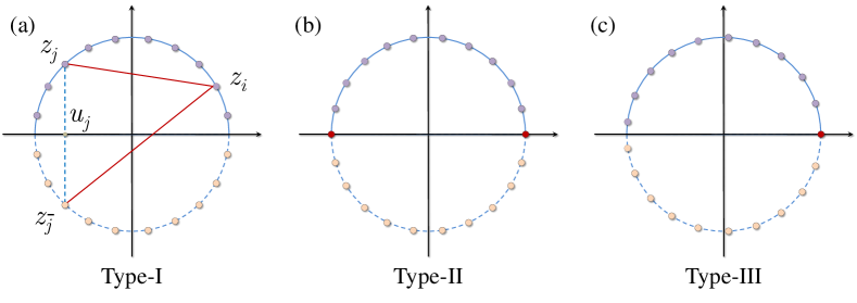
Figure 1: (Color online) Schematic of an open chain in the upper complex plane. The lattice sites and their mirror images locate on the upper and lower unit semicircles, respectively. They are symmetric with respect to the real axis. The two (brown) lines denote the chord distances $|z_{i}-z_{j}|$ and $|z_{i}-z_{\bar{j}}|$, respectively. (a)–(c) denote the three uniform cases: (a) type-I: $\theta_{j}=\frac{\pi}{L}(j-\frac{1}{2})$; (b) type-II: $\theta_{j}=\frac{\pi}{L+1}j$; (c) type-III: $\theta_{j}=\frac{2\pi}{2L+1}j$.

As shown in Ref. Ignacio10 , the infinite MPS (1) with coordinate choice $u_{j}=z_{j}=e^{i\frac{2\pi}{L}j}$, i.e., the case of equidistantly distributed spins on the whole unit circle, yields the ground state of the SU(2) Haldane-Shastry model Haldane88 ; Shastry88 , which is a paradigmatic spin-1/2 chain with PBC.

Now we demonstrate that our infinite MPS (1) with the image prescription, $u_{j}\equiv(z_{j}+z_{\bar{j}})/2$, describes a spin-1/2 chain with OBC. Let us first derive a parent Hamiltonian for which (2) is the exact ground state. Based on the CFT null field techniques, it was shown Anne11  that the decoupling equations satisfied by (1) lead to a set of operators annihilating the wave function (2), $\mathcal{C}_{i}^{a}|\Psi\rangle=0$ $\forall i,a$, where $\mathcal{C}_{i}^{a}=\frac{2}{3}\sum_{j(\neq i)}\frac{1}{u_{i}-u_{j}}(S_{j}^{a}+i\varepsilon_{abc}S_{i}^{b}S_{j}^{c})$ and $\varepsilon_{abc}$ is the Levi-Civita symbol [we assume summation over repeated indices and use the convention that $\sum_{j(\neq i)}$ is the sum over $j$, whereas $\sum_{i\neq j}$ is the sum over both $i$ and $j$]. When adapting to our present OBC setup, we consider the operators $\Lambda_{i}^{a}=\frac{2}{3}\sum_{j(\neq i)}(w_{ij}+w_{i\bar{j}})(S_{j}^{a}+i\varepsilon_{abc}S_{i}^{b}S_{j}^{c})$, where $w_{ij}=(z_{i}+z_{j})/(z_{i}-z_{j})$ and which also annihilate the wave function $|\Psi\rangle$, since $\Lambda_{i}^{a}=(z_{i}-z_{i}^{\ast})\mathcal{C}_{i}^{a}$. The parent Hamiltonian for (2) is then defined as $H=\frac{1}{8}\sum_{i,a}(\Lambda_{i}^{a})^{\dagger}\Lambda_{i}^{a}+\frac{L}{3}\mathbf{S}^{2}+E$, where $\mathbf{S}^{2}=\sum_{ij}\vec{S}_{i}\cdot\vec{S}_{j}$ is the total spin operator and $E=\frac{1}{16}\sum_{i\neq j}(w_{ij}^{2}+w_{i\bar{j}}^{2})-\frac{1}{4}L^{2}$. After some algebra Supp , we arrive at a long-range Heisenberg model

$$H = \sum_{i\neq j}\left[\frac{1}{|z_{i}-z_{j}|^{2}}+\frac{1}{|z_{i}-z_{\bar{j}}|^{2}}-\frac{w_{ij}(c_{i}-c_{j})}{12}\right.$$ (3)

$$\left.-\frac{w_{i\bar{j}}(c_{i}+c_{j})}{12}\right](\vec{S}_{i}\cdot\vec{S}_{j})$$

with ground-state energy $E$, where $c_{j}=w_{\bar{j}j}+\sum_{l(\neq j)}(w_{lj}+w_{\bar{l}j})$.

Three choices of the lattice coordinates deserve special attention (see Fig. 1): (i) type-I: $\theta_{j}=\frac{\pi}{L}(j-\frac{1}{2})$; (ii) type-II: $\theta_{j}=\frac{\pi}{L+1}j$; (iii) type-III: $\theta_{j}=\frac{2\pi}{2L+1}j$. For these three cases (termed as uniform cases afterwards), one obtains $w_{ij}(c_{i}-c_{j})+w_{i\bar{j}}(c_{i}+c_{j})=0$, $4$, and $2$, respectively. Accordingly, the parent Hamiltonians, after removing the (unimportant) total spin operator $\mathbf{S}^{2}$ and constant terms in (3), have purely inverse-square exchange interactions (between the spins and also their images), which coincide with the open Haldane-Shastry models first introduced in Refs. Simons94 ; Bernard95 . These uniform models are integrable and have highly degenerate multiplets in their energy spectrum Simons94 ; Bernard95 , similar to their periodic counterpart Haldane92 , see Fig. 2 for the full spectrum of the open and periodic Haldane-Shastry models with $L=6$. We postpone the discussion of this degeneracy until presenting the SU($n$) generalization of these models, where a unified treatment is possible. The Hamiltonian (3) with lattice coordinates other than the three uniform cases is an inhomogeneous generalization of the open Haldane-Shastry models and does not exhibit the huge degeneracy in the spectrum.

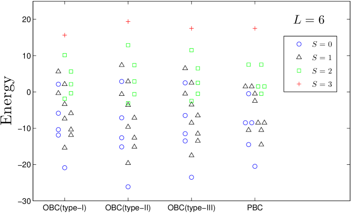
Figure 2: (Color online) The energy spectrum of the three types of spin-1/2 open Haldane-Shastry models and the spin-1/2 periodic Haldane-Shastry model ($H=\sum_{i\neq j}\frac{\vec{S}_{i}\cdot\vec{S}_{j}}{\sin^{2}[\pi(i-j)/L]}$) with $L=6$. All four models have highly degenerate multiplets in their energy spectrum. While the first excited states of the periodic model are degenerate singlet and triplet (due to two free spin-1/2 spinons), the open models do not have this degeneracy, indicating the importance of the boundary effect.

Spin correlator.— A nontrivial application of the infinite MPS formulation is that, for the wave function (2), the spin correlation functions can be computed easily. Since $\mathcal{C}_{i}^{a}|\Psi\rangle=0$, one has $\langle\Psi|\sum_{a}S_{i}^{a}\mathcal{C}_{j}^{a}|\Psi\rangle=0$ and $\langle\Psi|\sum_{a}(\mathcal{C}_{j}^{a})^{\dagger}S_{i}^{a}|\Psi\rangle=0$ $\forall i,j$, which lead to a set of linear equations relating two-point correlators $C_{ij}+\sum_{l(\neq i,j)}\frac{u_{i}-u_{j}}{u_{i}-u_{l}}C_{jl}=-\frac{3}{4}$ Anne11 , where $C_{ij}\equiv\langle\Psi|\vec{S}_{i}\cdot\vec{S}_{j}|\Psi\rangle/\langle\Psi|\Psi\rangle$. These equations are sufficient for computing the two-point spin correlators for arbitrary choices of $\theta_{j}$ (both inhomogeneous and uniform cases). The generalization to arbitrary higher-order spin correlators is rather straightforward.

Most remarkably, for the type-I uniform case, these linear equations allow us to find an analytical expression for the two-point spin correlator Supp

$$C_{ij} = \frac{3(-1)^{i-j}\sin\theta_{i}\sin\theta_{j}}{L(\cos\theta_{i}-\cos\theta_{j})}\sum_{p=1}^{L/2}\sum_{q=0}^{p-1}g_{pq}[\cos(2p-1)\theta_{i}$$ (4)

$$\times\cos 2q\theta_{j}-\cos 2q\theta_{i}\cos(2p-1)\theta_{j}]$$

with

$$g_{pq}=\left\{\begin{array}[]{c}1\\ \prod_{m=1}^{p-1}\frac{4m-1}{4m+1}\\ 2\prod_{m=1}^{p-1}\frac{4m-1}{4m+1}\prod_{n=1}^{q}\frac{4n-3}{4n-1}\end{array}\right.\left.\begin{array}[]{c}p=1,q=0\\ p>1,q=0\\ p>1,q>0\end{array}\right..$$ (5)

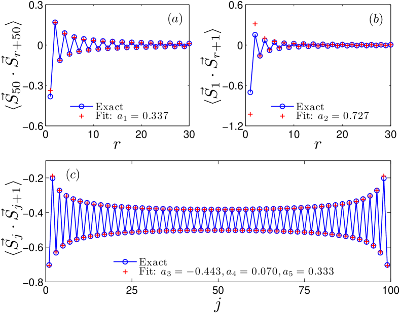
Figure 3: (Color online) Two-point spin correlators of the wave function (2) in the type-I uniform case with $L=100$. The blue circles are the exact results from (4), and the red crosses are fits with theoretical predictions based on the SU(2)₁ WZW model with free boundary condition (see text). (a) Two spins at lattice sites $50$ and $50+r$ are far from the boundary. (b) One of the spins lives at the boundary (the first spin). For (a) and (b), the first four points are excluded when computing the fits, since the theoretical predictions are valid for large $r$. (c) Two spins are nearest neighbors.

In Fig. 3 various correlators from (4) are compared with the theoretical predictions Eggert92 based on the SU(2)₁ Wess-Zumino-Witten (WZW) model with free boundary condition. When two spins at sites $j$ and $j+r$ are both far from the boundary, one expects that the correlator $C_{j,j+r}$ recovers the result for PBC Gebhard87 , $C_{j,j+r}\simeq a_{1}(-1)^{r}/[\frac{2L}{\pi}\sin(\frac{\pi r}{2L})]\propto(-1)^{r}/r$ for large $r$, where $a_{1}$ is a constant. However, if one of the two spins (say, the one at site $j$) is very close to the boundary, the theory developed in Ref. Eggert92 predicts $C_{j,j+r}\simeq a_{2}(-1)^{r}[\frac{L}{\pi}\sin(\frac{\pi r}{L})]^{1/2}/[\frac{2L}{\pi}\sin(\frac{\pi r}{2L})]^{2}\propto(-1)^{r}/r^{3/2}$ ($a_{2}$: nonuniversal constant) with a boundary critical exponent $\eta=3/2$ that differs from $\eta=1$ in the bulk. For the correlator between nearest neighbors, it was predicted Ng96 ; Laflorencie06 that $C_{j,j+1}=a_{3}+a_{4}/[\frac{L}{\pi}\sin(\frac{\pi j}{L})]^{2}+a_{5}(-1)^{j}/[\frac{L}{\pi}\sin(\frac{\pi j}{L})]^{K}$, where $K$ is the Luttinger parameter, $K=1/2$, and $a_{3},a_{4},a_{5}$ are constants. We treat the nonuniversal constants $a_{1},\ldots,a_{5}$ as fitting parameters and find excellent agreement between the exact result (4) and the SU(2)₁ WZW predictions (see Fig. 3).

Entanglement entropy.— To provide further support that the wave function (2) is relevant for open critical chains, we numerically compute the Rényi entropy $S^{(2)}(l)=-\ln\mathrm{Tr}\rho_{l}^{2}$ via Monte Carlo method Ignacio10 ; Hastings10 , where $\rho_{l}$ is the reduced density matrix of the first $l$ spins. In Fig. 4 we plot $S^{(2)}(l)$ for the wave function (2) in the type-I uniform case with $L=100$. For open spin-1/2 chains described by the SU(2)₁ WZW model with free boundary condition, one expects the Rényi entropy to be Laflorencie06

$$S^{(2)}(l)=\frac{c}{8}\ln\left[\frac{L}{\pi}\sin\left(\frac{\pi l}{L}\right)\right]+c_{2}+\frac{(-1)^{l}f_{2}}{[\frac{L}{\pi}\sin(\frac{\pi l}{L})]^{\frac{K}{2}}}$$ (6)

with central charge $c=1$, Luttinger parameter $K=1/2$, and $c_{2},f_{2}$ nonuniversal constants. Fixing $c=1$ and $K=1/2$ and treating $c_{2},f_{2}$ as fitting parameters, the numerical results are in good agreement with the theoretical prediction (see Fig. 4). For the type-II and type-III uniform cases, we have verified via Monte Carlo simulations that their Rényi entropies also agree with (6), suggesting that they all belong to the SU(2)₁ WZW model with free boundary condition.

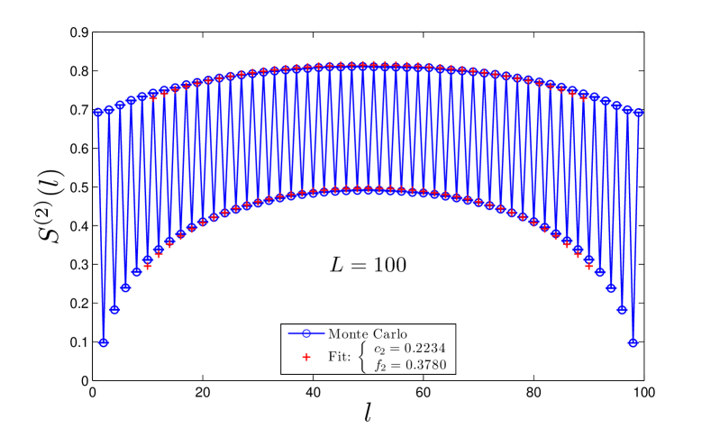
Figure 4: (Color online) Rényi entropy $S^{(2)}(l)$ of the wave function (2) in type-I uniform case with $L=100$ as a function of the subsystem size $l$. The blue circles (with errorbars) are obtained from Monte Carlo simulations and the red crosses are fits based on the theoretical prediction (6) of the SU(2)₁ WZW model. The fit is computed with $l\in[10,90]$, as (6) is valid for large subsystem sizes.

SU(n) generalization.— As a further application we generalize the above SU(2) example to the SU($n$) case. For the SU($n$)₁ WZW model, the infinite MPS have been proposed in Refs. Tu14b ; Bondesan14 . Here we take in all sites SU($n$) spins transforming under fundamental representations, with local basis denoted by $|\alpha\rangle$ ($\alpha=1,\ldots,n$). Following Ref. Tu14b , the CFT fields for defining the infinite MPS (1) are given by $A^{\alpha}(u)=\kappa_{\alpha}:e^{i\vec{m}_{\alpha}\cdot\vec{\phi}(u)/\sqrt{2}}:$, where $\vec{m}_{\alpha}$ is a $(n-1)$-component vector denoting the fundamental weight of $|\alpha\rangle$ (e.g., $\vec{m}_{1,2}=(\pm 1,1/\sqrt{3})$ and $\vec{m}_{3}=(0,2/\sqrt{3})$ for SU(3), see Tu14b ), $\vec{\phi}(u)$ is a vector of $n-1$ chiral bosonic fields, and $\kappa_{\alpha}$ is a Klein factor, commuting with vertex operators and satisfying $\{\kappa_{\alpha},\kappa_{\alpha^{\prime}}\}=2\delta_{\alpha\alpha^{\prime}}$. Evaluating the CFT correlator (1), the SU($n$) wave function takes a simple Jastrow form, $\Psi_{\mathrm{SU(}n\mathrm{)}}(\alpha_{1},\ldots,\alpha_{L})=\mathrm{sgn}(x_{1}^{(1)},\ldots,x_{L/n}^{(1)},\ldots,x_{1}^{(n)},\ldots,x_{L/n}^{(n)})\delta_{\sum_{i}\vec{m}_{\alpha_{i}}=0}\prod_{i<j}(u_{i}-u_{j})^{\delta_{\alpha_{i}\alpha_{j}}}$ (sgn: signature of a permutation), where $x_{k}^{(\alpha)}$ ($k=1,\ldots,L/n$), for a given configuration $|\alpha_{1},\ldots,\alpha_{L}\rangle$, is the position of the $k$th spin in the state $|\alpha\rangle$.

Following a procedure similar to the SU(2) case Supp , we obtain a two-body parent Hamiltonian for $\Psi_{\mathrm{SU(}n)}$, $H=\sum_{i\neq j}\left[\frac{1}{|z_{i}-z_{j}|^{2}}+\frac{1}{|z_{i}-z_{\bar{j}}|^{2}}-\frac{w_{ij}(c_{i}-c_{j})+w_{i\bar{j}}(c_{i}+c_{j})}{4(n+1)}\right](\vec{t}_{i}\cdot\vec{t}_{j})$, where $t^{a}$ ($a=1,\ldots,n^{2}-1$) are SU($n$) generators in the fundamental representation, normalized as $\mathrm{tr}(t^{a}t^{b})=\frac{1}{2}\delta_{ab}$. The three uniform choices of $\theta_{j}$, very much the same as the SU(2) cases, bring the parent Hamiltonian into SU($n$) open Haldane-Shastry models

$$H_{\mathrm{SU(}n\mathrm{)}}=\sum_{i\neq j}\left[\frac{1}{|z_{i}-z_{j}|^{2}}+\frac{1}{|z_{i}-z_{\bar{j}}|^{2}}\right](\vec{t}_{i}\cdot\vec{t}_{j})$$ (7)

with purely inverse-square interactions.

Motivated by the SU(2) result Bernard95 , we have numerically observed that the full spectrum of the SU($n$) open Haldane-Shastry model (7) is described by the formula, $H_{\mathrm{SU(}n\mathrm{)}}|\{m_{i}\}\rangle=[E_{0}+\sum_{i=1}^{M}E(m_{i})]|\{m_{i}\}\rangle,$ where $E_{0}=-\frac{n-1}{8n}[\sum_{i\neq j}(w_{ij}^{2}+w_{i\bar{j}}^{2})-2L(L-1)]$ and $E(m_{i})=\frac{1}{2}(m_{i}^{2}-\frac{1}{4}N^{2})$ ($N=2L$, $2L+2$, and $2L+1$ for the three uniform cases, respectively), $M$ is an integer satisfying $M\in[0,\frac{n-1}{n}L]$, and $m_{i}$ are distinct integer/half-integer rapidities ($1\leq m_{i}\leq L-1$, $2\leq m_{i}\leq L$, and $\frac{3}{2}\leq m_{i}\leq L-\frac{1}{2}$ for each individual uniform case), satisfying the generalized Pauli principle which is the same as that for the SU($n$) Haldane-Shastry model with PBC Kawakami92 ; Ha92 : only those sets $\{m_{1},\ldots,m_{M}\}$ without $n$ or more consecutive integers/half-integers are allowed Haldane92 .

Twisted Yangian.— Our numerical results also indicate that the “supermultiplet” structure in the spectrum, which already shows up in the SU(2) case (see Fig. 2), persists in the SU($n$) open Haldane-Shastry models (7). To explain this degeneracy, we slightly generalize the monodromy matrix found for the spin-1/2 open Haldane-Shastry models Bernard95 to the SU($n$) case. Through a third-order expansion of the monodromy matrix Supp , we obtain the nontrivial conserved charge responsible for the SU($n$) open Haldane-Shastry models (7)

$$Q^{a} = \sum_{k}t_{k}^{a}(w_{k\bar{k}}^{2}+\gamma_{1}w_{k0}^{2})-\gamma_{2}\sum_{i\neq j\neq k}(w_{jk}+w_{j\bar{k}})$$ (8)

$$\times(w_{ij}-w_{i\bar{j}})t_{k}^{a}P_{jk}P_{ij},$$

where $w_{k0}=(z_{k}+1)/(z_{k}-1)$, $P_{ij}$ swaps the spin states at site $i$ and $j$ (more explicitly, $P_{ij}=2\vec{t}_{i}\cdot\vec{t}_{j}+\frac{1}{n}$) and $\gamma_{1}$ and $\gamma_{2}$ are given by (i) type-I: $\gamma_{1}=0$, $\gamma_{2}=\frac{1}{2}$; (ii) type-II: $\gamma_{1}=0$, $\gamma_{2}=\frac{1}{10}$; (iii) type III: $\gamma_{1}=1$, $\gamma_{2}=\frac{1}{2}$, respectively. The conserved charge $Q^{a}$ and the total spin $T^{a}\equiv\sum_{j}t_{j}^{a}$ both commute with (7), but $Q^{a}$ does not commute with the SU($n$) Casimir operator $\sum_{a}T^{a}T^{a}$. This explains the appearance of degenerate eigenstates with different SU($n$) representations. As the monodromy matrix relevant for these models (with open boundaries) satisfies the reflection equation Sklyanin88 , the algebraic structure of the SU($n$) open Haldane-Shastry models (7) is the twisted Yangian Olshanski92 . Thus, the conserved charges $Q^{a}$ and $T^{a}$ form the lowest twisted Yangian generators.

Conclusions.— In this Rapid Communication, we have shown that infinite MPS with the image prescription are relevant for 1D critical chains with OBC, by presenting a spin-1/2 example, as well as its SU($n$) generalization. We have constructed inhomogeneous open Haldane-Shastry models as their parent Hamiltonians, including the three open Haldane-Shastry models as special uniform cases. For the type-I spin-1/2 open Haldane-Shastry model, an exact expression for the two-point spin correlator has been derived and compared with theoretical predictions, supporting that the low-energy effective theory is the SU(2)₁ WZW model with free boundary condition. We also characterize the full spectrum of the SU($n$) open Haldane-Shastry models and determine the twisted Yangian generators responsible for the highly degenerate multiplets in the energy spectrum. The present infinite MPS with open boundaries is readily applicable to any boundary CFT for finding their lattice discretizations. As an outlook, we expect that the infinite MPS with OBC could be very useful for proposing trial wave functions for single-impurity Kondo problems, where boundary CFT are known Affleck90 ; Affleck91 to play an important role.

Acknowledgment.— We acknowledge J. I. Cirac and A. E. B. Nielsen for helpful discussions. This work has been supported by the EU project SIQS, FIS2012-33642, QUITEMAD (CAM), the Severo Ochoa Program, and the Fulbright grant PRX14/00352.

Supplemental Material

Appendix A Inhomogeneous open Haldane-Shastry models

In this Section, we provide details on the derivation of the spin-1/2 inhomogeneous open Haldane-Shastry model and its SU($n$) generalization.

To construct the spin-1/2 inhomogeneous open Haldane-Shastry model, we use the operators annihilating the spin-1/2 open infinite MPS

$$\Lambda_{i}^{a}=\frac{2}{3}\sum_{j(\neq i)}(w_{ij}+w_{i\bar{j}})(S_{j}^{a}+i\varepsilon_{abc}S_{i}^{b}S_{j}^{c}),$$ (1)

to build a positive semidefinite operator

$$\sum_{a}(\Lambda_{i}^{a})^{\dagger}\Lambda_{i}^{a} = \frac{4}{9}\sum_{j,k(\neq i)}(w_{ij}^{\ast}+w_{i\bar{j}}^{\ast})(w_{ik}+w_{i\bar{k}})(S_{j}^{a}-i\varepsilon_{abc}S_{i}^{b}S_{j}^{c})(S_{k}^{a}+i\varepsilon_{ade}S_{i}^{d}S_{k}^{e})$$ (2)

$$= -\frac{4}{9}\sum_{j,k(\neq i)}(w_{ij}+w_{i\bar{j}})(w_{ik}+w_{i\bar{k}})(\vec{S}_{j}\cdot\vec{S}_{k}-2i\varepsilon_{abc}S_{i}^{a}S_{j}^{b}S_{k}^{c}+\varepsilon_{abc}\varepsilon_{ade}S_{i}^{b}S_{i}^{d}S_{j}^{c}S_{k}^{e})$$

$$= -\frac{4}{9}\sum_{j,k(\neq i)}(w_{ij}+w_{i\bar{j}})(w_{ik}+w_{i\bar{k}})(\vec{S}_{j}\cdot\vec{S}_{k}-2i\varepsilon_{abc}S_{i}^{a}S_{j}^{b}S_{k}^{c}+\frac{1}{4}\varepsilon_{abc}\varepsilon_{abe}S_{j}^{c}S_{k}^{e}+\frac{i}{2}\varepsilon_{abc}\varepsilon_{ade}\varepsilon_{bdf}S_{i}^{f}S_{j}^{c}S_{k}^{e})$$

$$= -\frac{2}{3}\sum_{j,k(\neq i)}(w_{ij}+w_{i\bar{j}})(w_{ik}+w_{i\bar{k}})(\vec{S}_{j}\cdot\vec{S}_{k}-i\varepsilon_{abc}S_{i}^{a}S_{j}^{b}S_{k}^{c})$$

$$= -\frac{2}{3}\sum_{j(\neq i)}(w_{ij}+w_{i\bar{j}})^{2}(\frac{3}{4}+\vec{S}_{i}\cdot\vec{S}_{j})-\frac{2}{3}\sum_{j\neq k(\neq i)}(w_{ij}+w_{i\bar{j}})(w_{ik}+w_{i\bar{k}})(\vec{S}_{j}\cdot\vec{S}_{k}),$$

where we have used $w_{ij}^{\ast}=-w_{ij}$, $S^{b}S^{d}=\frac{1}{4}\delta_{ab}+\frac{i}{2}\varepsilon_{abc}S^{c}$, $\varepsilon_{abc}\varepsilon_{abd}=2\delta_{cd}$, and $\varepsilon_{abc}\varepsilon_{ade}\varepsilon_{bdf}=\varepsilon_{cef}$. Then, we obtain

$$\sum_{i,a}(\Lambda_{i}^{a})^{\dagger}\Lambda_{i}^{a}=-\frac{2}{3}\sum_{i\neq j}(w_{ij}+w_{i\bar{j}})^{2}(\frac{3}{4}+\vec{S}_{i}\cdot\vec{S}_{j})-\frac{2}{3}\sum_{j\neq k}\left(\sum_{i(\neq j,k)}(w_{ij}+w_{i\bar{j}})(w_{ik}+w_{i\bar{k}})\right)(\vec{S}_{j}\cdot\vec{S}_{k}).$$ (3)

The following cyclic identity is the key for simplifying (3):

$$(w_{ij}+w_{i\bar{j}})(w_{ik}+w_{i\bar{k}})+(w_{ji}+w_{j\bar{\imath}})(w_{jk}+w_{j\bar{k}})+(w_{ki}+w_{k\bar{\imath}})(w_{kj}+w_{k\bar{j}})=4.$$ (4)

By using this identity, we obtain

$$\sum_{i(\neq j,k)}(w_{ij}+w_{i\bar{j}})(w_{ik}+w_{i\bar{k}}) = \sum_{i(\neq j,k)}[4-(w_{ji}+w_{j\bar{\imath}})(w_{jk}+w_{j\bar{k}})-(w_{ki}+w_{k\bar{\imath}})(w_{kj}+w_{k\bar{j}})]$$ (5)

$$= 4(L-2)-(w_{jk}+w_{j\bar{k}})\sum_{i(\neq j,k)}(w_{ji}+w_{j\bar{\imath}})-(w_{kj}+w_{k\bar{j}})\sum_{i(\neq j,k)}(w_{ki}+w_{k\bar{\imath}})$$

$$= 4(L-2)+2(w_{jk}^{2}+w_{j\bar{k}}^{2})-(w_{jk}+w_{j\bar{k}})\left[w_{j\bar{j}}+\sum_{i(\neq j)}(w_{ji}+w_{j\bar{\imath}})\right]$$

$$-(w_{kj}+w_{k\bar{j}})\left[w_{k\bar{k}}+\sum_{i(\neq k)}(w_{ki}+w_{k\bar{\imath}})\right]+w_{j\bar{j}}(w_{jk}+w_{j\bar{k}})+w_{k\bar{k}}(w_{kj}+w_{k\bar{j}})$$

$$= (4L-6)+2(w_{jk}^{2}+w_{j\bar{k}}^{2})+w_{jk}(c_{j}-c_{k})+w_{j\bar{k}}(c_{j}+c_{k}),$$

where we have defined $c_{j}\equiv w_{\bar{j}j}+\sum_{i(\neq j)}(w_{ij}+w_{\bar{\imath}j})$ and have used $w_{j\bar{j}}(w_{jk}+w_{j\bar{k}})+w_{k\bar{k}}(w_{kj}+w_{k\bar{j}})=2$ (the latter can be easily proved by using the cyclic identity $w_{ij}w_{ik}+w_{ji}w_{jk}+w_{ki}w_{kj}=1$).

By substituting (5) into (3), we arrive at

$$\sum_{i,a}(\Lambda_{i}^{a})^{\dagger}\Lambda_{i}^{a} = -\frac{2}{3}\sum_{i\neq j}(w_{ij}+w_{i\bar{j}})^{2}(\frac{3}{4}+\vec{S}_{i}\cdot\vec{S}_{j})$$ (6)

$$-\frac{2}{3}\sum_{j\neq k}\left[(4L-6)+2(w_{jk}^{2}+w_{j\bar{k}}^{2})+w_{jk}(c_{j}-c_{k})+w_{j\bar{k}}(c_{j}+c_{k})\right](\vec{S}_{j}\cdot\vec{S}_{k})$$

$$= 8\sum_{i\neq j}\left[\frac{1}{|z_{i}-z_{j}|^{2}}+\frac{1}{|z_{i}-z_{\bar{j}}|^{2}}-\frac{w_{ij}(c_{i}-c_{j})+w_{i\bar{j}}(c_{i}+c_{j})}{12}\right](\vec{S}_{i}\cdot\vec{S}_{j})$$

$$-\frac{8L}{3}\mathbf{S}^{2}-\frac{1}{2}\sum_{i\neq j}(w_{ij}+w_{i\bar{j}})^{2}+2L^{2},$$

where we have used $w_{ij}^{2}=1-\frac{4}{|z_{i}-z_{j}|^{2}}$.

Then, the spin-1/2 inhomogeneous open Haldane-Shastry model is defined by

$$H = \frac{1}{8}\sum_{i,a}(\Lambda_{i}^{a})^{\dagger}\Lambda_{i}^{a}+\frac{L}{3}\mathbf{S}^{2}+E$$ (7)

$$= \sum_{i\neq j}\left[\frac{1}{|z_{i}-z_{j}|^{2}}+\frac{1}{|z_{i}-z_{\bar{j}}|^{2}}-\frac{w_{ij}(c_{i}-c_{j})+w_{i\bar{j}}(c_{i}+c_{j})}{12}\right](\vec{S}_{i}\cdot\vec{S}_{j}),$$

whose ground-state energy $E$ is given by $E=\frac{1}{16}\sum_{i\neq j}(w_{ij}+w_{i\bar{j}})^{2}-\frac{1}{4}L^{2}$.

The derivation of the SU($n$) inhomogeneous open Haldane-Shastry model follows the similar steps for the spin-1/2 case. The operators annihilating the SU($n$) infinite MPS are given by suppTu14b ; suppBondesan14

$$\Lambda_{i}^{a}=\frac{n+2}{2(n+1)}\sum_{j(\neq i)}(w_{ij}+w_{i\bar{j}})[t_{j}^{a}+(\frac{n}{n+2}d_{abc}+if_{abc})t_{i}^{b}t_{j}^{c}],$$ (8)

where $d_{abc}$ and $f_{abc}$ are the SU($n$) totally symmetry tensor and the totally antisymmetric structure constant, respectively. Similar to the spin-1/2 case, we consider the positive semidefinite operator

$$\sum_{a}(\Lambda_{i}^{a})^{\dagger}\Lambda_{i}^{a} = \frac{(n+2)^{2}}{4(n+1)^{2}}\sum_{j,k(\neq i)}(w_{ij}^{\ast}+w_{i\bar{j}}^{\ast})(w_{ik}+w_{i\bar{k}})[t_{j}^{a}+(\frac{n}{n+2}d_{abc}+if_{abc})t_{i}^{b}t_{j}^{c}][t_{k}^{a}+(\frac{n}{n+2}d_{ade}+if_{ade})t_{i}^{d}t_{k}^{e}]$$ (9)

$$= \sum_{j,k(\neq i)}(w_{ij}^{\ast}+w_{i\bar{j}}^{\ast})(w_{ik}+w_{i\bar{k}})[\frac{n+2}{2(n+1)}(\vec{t}_{j}\cdot\vec{t}_{k})+\frac{n}{2(n+1)}d_{abc}t_{i}^{a}t_{j}^{b}t_{k}^{c}-\frac{n+2}{2(n+1)}if_{abc}t_{i}^{a}t_{j}^{b}t_{k}^{c}]$$

$$= -\sum_{j(\neq i)}(w_{ij}+w_{i\bar{j}})^{2}\left[\frac{(n-1)(n+2)}{4n}+\frac{(n-1)(n+2)}{2(n+1)}(\vec{t}_{i}\cdot\vec{t}_{j})\right]$$

$$-\sum_{j\neq k(\neq i)}(w_{ij}+w_{i\bar{j}})(w_{ik}+w_{i\bar{k}})\left[\frac{n+2}{2(n+1)}(\vec{t}_{j}\cdot\vec{t}_{k})+\frac{n}{2(n+1)}d_{abc}t_{i}^{a}t_{j}^{b}t_{k}^{c}\right],$$

where we have extensively used the identities listed in the Appendix A in Ref. suppTu14b . Notice that

$$\sum_{i\neq j\neq k}(w_{ij}+w_{i\bar{j}})(w_{ik}+w_{i\bar{k}})d_{abc}t_{i}^{a}t_{j}^{b}t_{k}^{c}$$ (10)

$$= \frac{1}{3}\sum_{i\neq j\neq k}[(w_{ij}+w_{i\bar{j}})(w_{ik}+w_{i\bar{k}})+(w_{ji}+w_{j\bar{\imath}})(w_{jk}+w_{j\bar{k}})+(w_{ki}+w_{k\bar{\imath}})(w_{kj}+w_{k\bar{j}})]d_{abc}t_{i}^{a}t_{j}^{b}t_{k}^{c}$$

$$= \frac{4}{3}\sum_{i\neq j\neq k}d_{abc}t_{i}^{a}t_{j}^{b}t_{k}^{c}$$

$$= \frac{4}{3}d_{abc}T^{a}T^{b}T^{c}-\frac{2(n^{2}-4)}{n}T^{a}T^{a}+\frac{2(n^{2}-1)(n^{2}-4)}{3n^{2}}L,$$

where $T^{a}=\sum_{i}t_{i}^{a}$. Together with (5), we obtain

$$\sum_{i,a}(\Lambda_{i}^{a})^{\dagger}\Lambda_{i}^{a} = -\sum_{i\neq j}(w_{ij}+w_{i\bar{j}})^{2}\left[\frac{(n-1)(n+2)}{4n}+\frac{(n-1)(n+2)}{2(n+1)}(\vec{t}_{i}\cdot\vec{t}_{j})\right]$$

$$-\sum_{i\neq j\neq k}(w_{ij}+w_{i\bar{j}})(w_{ik}+w_{i\bar{k}})\left[\frac{n+2}{2(n+1)}(\vec{t}_{j}\cdot\vec{t}_{k})+\frac{n}{2(n+1)}d_{abc}t_{i}^{a}t_{j}^{b}t_{k}^{c}\right]$$

$$= 2(n+2)\sum_{i\neq j}\left[\frac{1}{|z_{i}-z_{j}|^{2}}+\frac{1}{|z_{i}-z_{\bar{j}}|^{2}}-\frac{w_{ij}(c_{i}-c_{j})+w_{i\bar{j}}(c_{i}+c_{j})}{4(n+1)}\right](\vec{t}_{i}\cdot\vec{t}_{j})$$

$$-\frac{2n}{3(n+1)}d_{abc}T^{a}T^{b}T^{c}-\frac{2(n+2)L}{n+1}T^{a}T^{a}-\frac{(n-1)(n+2)}{4n}\sum_{i\neq j}(w_{ij}^{2}+w_{i\bar{j}}^{2})$$

$$+\frac{(n-1)(n+2)}{6n}L(6L+n-2).$$

Then, the SU($n$) inhomogeneous open Haldane-Shastry model can be defined as

$$H = \frac{1}{2(n+2)}\sum_{i,a}(\Lambda_{i}^{a})^{\dagger}\Lambda_{i}^{a}+\frac{n}{3(n+1)(n+2)}d_{abc}T^{a}T^{b}T^{c}+\frac{L}{n+1}T^{a}T^{a}+E$$ (12)

$$= \sum_{i\neq j}\left[\frac{1}{|z_{i}-z_{j}|^{2}}+\frac{1}{|z_{i}-z_{\bar{j}}|^{2}}-\frac{w_{ij}(c_{i}-c_{j})+w_{i\bar{j}}(c_{i}+c_{j})}{4(n+1)}\right](\vec{t}_{i}\cdot\vec{t}_{j}),$$

whose ground-state energy $E$ is given by $E=\frac{n-1}{8n}\sum_{i\neq j}(w_{ij}^{2}+w_{i\bar{j}}^{2})-\frac{n-1}{12n}L(6L+n-2)$.

Appendix B Two-point spin correlation function for the type-I spin-1/2 open Haldane-Shastry model

In this Section, we derive the exact expression of the two-point spin correlation function for the type-I spin-1/2 open Haldane-Shastry model.

As we mentioned in the main text, the two-point spin correlation function $C_{ij}=\langle\Psi|\vec{S}_{i}\cdot\vec{S}_{j}|\Psi\rangle/\langle\Psi|\Psi\rangle$ satisfies the following linear equations:

$$\frac{1}{u_{i}-u_{j}}C_{ij}+\sum_{l(\neq i,j)}\frac{1}{u_{i}-u_{l}}C_{jl}=-\frac{3}{4}\frac{1}{u_{i}-u_{j}},\text{ \ }\forall i,j$$ (13)

where $u_{j}=\cos\theta_{j}$. Since $|\Psi\rangle$ is a spin singlet, $\sum_{j=1}^{L}\vec{S}_{j}|\Psi\rangle=0$, the correlator also satisfies

$$\sum_{j(\neq i)}C_{ij}=-\frac{3}{4}.$$ (14)

For instance, if one wants to determine the correlators involving the first spin, one could write down the $L-1$ linear equations (relating $C_{1j}$, $j=2,\ldots,L$) in a matrix form:

$$\begin{pmatrix}-\frac{1}{u_{1}-u_{2}}&\frac{1}{u_{2}-u_{3}}&\frac{1}{u_{2}-u_{4}}&\cdots&\frac{1}{u_{2}-u_{L}}\\ \frac{1}{u_{3}-u_{2}}&-\frac{1}{u_{1}-u_{3}}&\frac{1}{u_{3}-u_{4}}&\cdots&\frac{1}{u_{3}-u_{L}}\\ \frac{1}{u_{4}-u_{2}}&\frac{1}{u_{4}-u_{3}}&-\frac{1}{u_{1}-u_{4}}&\cdots&\frac{1}{u_{4}-u_{L}}\\ \vdots&\vdots&\vdots&\ddots&\vdots\\ \frac{1}{u_{L}-u_{2}}&\frac{1}{u_{L}-u_{3}}&\frac{1}{u_{L}-u_{4}}&\cdots&-\frac{1}{u_{1}-u_{L}}\end{pmatrix}\begin{pmatrix}C_{12}\\ C_{13}\\ C_{14}\\ \vdots\\ C_{1L}\end{pmatrix}=-\frac{3}{4}\begin{pmatrix}\frac{1}{u_{2}-u_{1}}\\ \frac{1}{u_{3}-u_{1}}\\ \frac{1}{u_{4}-u_{1}}\\ \vdots\\ \frac{1}{u_{L}-u_{1}}\end{pmatrix}.$$ (15)

The correlators involving other spins can be solved in a similar fashion. For the moment, we carry out the derivations based on (15) for ease of notation and, in the end, extend the final result to the most general case.

For the type-I case with $\theta_{j}=\frac{\pi}{L}(j-\frac{1}{2})$, the following sum identity is very useful:

$$\sum_{j(\neq i)}\frac{1}{u_{j}-u_{i}}\cos m\theta_{j}=\frac{2(L-m)\sin\theta_{i}\sin m\theta_{i}-\cos\theta_{i}\cos m\theta_{i}}{2\sin^{2}\theta_{i}},$$ (16)

where $m$ is an integer and $m\in[0,2L]$.

For the $l$-th row in (15), we multiply $\cos m\theta_{l+1}$ and then sum over all the linear equations. By using (16), we obtain

$$\sum_{j=2}^{L}\left[\frac{\cos m\theta_{1}+\cos m\theta_{j}}{\cos\theta_{1}-\cos\theta_{j}}-\frac{2(L-m)\sin\theta_{j}\sin m\theta_{j}-\cos\theta_{j}\cos m\theta_{j}}{2\sin^{2}\theta_{j}}\right]C_{1j}=\frac{3}{8}\frac{2(L-m)\sin\theta_{1}\sin m\theta_{1}-\cos\theta_{1}\cos m\theta_{1}}{\sin^{2}\theta_{1}},$$ (17)

where $m\in[0,2L]$. For $m=0$, this yields

$$\sum_{j=2}^{L}\left(\frac{2}{\cos\theta_{1}-\cos\theta_{j}}+\frac{\cos\theta_{j}}{2\sin^{2}\theta_{j}}\right)C_{1j}=-\frac{3}{8}\frac{\cos\theta_{1}}{\sin^{2}\theta_{1}}.$$ (18)

When multiplying (18) by $\cos m\theta_{1}$ and then subtracting with (17), we obtain

$$\sum_{j=2}^{L}\left[\frac{\cos m\theta_{j}-\cos m\theta_{1}}{\cos\theta_{1}-\cos\theta_{j}}-\frac{2(L-m)\sin\theta_{j}\sin m\theta_{j}+\cos\theta_{j}(\cos m\theta_{1}-\cos m\theta_{j})}{2\sin^{2}\theta_{j}}\right]C_{1j}=\frac{3}{4}\frac{(L-m)\sin m\theta_{1}}{\sin\theta_{1}}.$$ (19)

Manipulating three consecutive linear equations [taking $m-1$, $m$, and $m+1$ in (19)], we arrive at

$$\sum_{j(\neq 1)}\left[(2L-2m+1)\frac{\cos(m+1)\theta_{j}}{\sin^{2}\theta_{j}}-(2L-2m-1)\frac{\cos(m-1)\theta_{j}}{\sin^{2}\theta_{j}}\right](\cos\theta_{1}-\cos\theta_{j})C_{1j}=3\cos m\theta_{1},$$ (20)

which we have verified to hold for $m\in[0,2L]$.

In general, the two-point spin correlator satisfies the following equation:

$$\sum_{j(\neq i)}\left[(2L-2m+1)\frac{\cos(m+1)\theta_{j}}{\sin^{2}\theta_{j}}-(2L-2m-1)\frac{\cos(m-1)\theta_{j}}{\sin^{2}\theta_{j}}\right](\cos\theta_{i}-\cos\theta_{j})C_{ij}=3\cos m\theta_{i},$$ (21)

where $m\in[0,2L]$.

In practice, finding the analytical form of $C_{ij}$ directly from (21) does not seem to be a simple task. Here we adopt an approach used in Ref. suppKuramotoBook to determine the analytical form of $C_{ij}$ for a few finite-size chains, from which a well-educated guess helps to solve (21).

In the hardcore boson basis, the type-I open Haldane-Shastry ground state is written as

$$|\Psi\rangle=\sum_{x_{1}<\ldots<x_{L/2}}\Psi(x_{1},\ldots,x_{L/2})S_{x_{1}}^{+}\cdots S_{x_{L/2}}^{+}|0\rangle,$$ (22)

where

$$\Psi(x_{1},\ldots,x_{L/2})=(-1)^{\sum_{i=1}^{L/2}x_{i}}\prod_{l=1}^{L/2}\sin\theta_{x_{l}}\prod_{1\leq i<j\leq L/2}(\cos\theta_{x_{i}}-\cos\theta_{x_{j}})^{2}.$$ (23)

Here $x_{1},\ldots,x_{L/2}$ denote the positions of the hardcore bosons (up spins).

The norm of (22) is given by

$$\langle\Psi|\Psi\rangle = \sum_{x_{1}<\ldots<x_{L/2}}|\Psi(x_{1},\ldots,x_{L/2})|^{2}$$ (24)

$$= \frac{1}{(L/2)!}\sum_{x_{1},\ldots,x_{L/2}}\prod_{l=1}^{L/2}\sin^{2}\theta_{x_{l}}\prod_{1\leq i<j\leq L/2}(\cos\theta_{x_{i}}-\cos\theta_{x_{j}})^{4}$$

$$= \frac{1}{(L/2)!}\sum_{x_{1},\ldots,x_{L/2}}\prod_{l=1}^{L/2}\sin^{2}\theta_{x_{l}}\det\begin{pmatrix}1&\cos\theta_{x_{1}}&\cos^{2}\theta_{x_{1}}&\cos^{3}\theta_{x_{1}}&\cdots&\cos^{L-1}\theta_{x_{1}}\\ 0&1&2\cos\theta_{x_{1}}&3\cos^{2}\theta_{x_{1}}&\cdots&(L-1)\cos^{L-2}\theta_{x_{1}}\\ 1&\cos\theta_{x_{2}}&\cos^{2}\theta_{x_{2}}&\cos^{3}\theta_{x_{2}}&\cdots&\cos^{L-1}\theta_{x_{2}}\\ 0&1&2\cos\theta_{x_{2}}&3\cos^{2}\theta_{x_{2}}&\cdots&(L-1)\cos^{L-2}\theta_{x_{2}}\\ \vdots&\vdots&\vdots&\vdots&\ddots&\vdots\\ 1&\cos\theta_{x_{L/2}}&\cos^{2}\theta_{x_{L/2}}&\cos^{3}\theta_{x_{L/2}}&\cdots&\cos^{L-1}\theta_{x_{L/2}}\\ 0&1&2\cos\theta_{x_{L/2}}&3\cos^{2}\theta_{x_{L/2}}&\cdots&(L-1)\cos^{L-2}\theta_{x_{L/2}}\end{pmatrix},$$

where in the last step we have used the Confluent Alternant identity suppKuramotoBook

$$\prod_{1\leq i<j\leq M}(y_{i}-y_{j})^{4}=\det\begin{pmatrix}1&y_{1}&y_{1}^{2}&y_{1}^{3}&\cdots&y_{1}^{M-1}\\ 0&1&2y_{1}&3y_{1}^{2}&\cdots&(M-1)y_{1}^{M-2}\\ 1&y_{2}&y_{2}^{2}&y_{2}^{3}&\cdots&y_{2}^{M-1}\\ 0&1&2y_{2}&3y_{2}^{2}&\cdots&(M-1)y_{2}^{M-2}\\ \vdots&\vdots&\vdots&\vdots&\ddots&\vdots\\ 1&y_{M}&y_{M}^{2}&y_{M}^{3}&\cdots&y_{M}^{M-1}\\ 0&1&2y_{M}&3y_{M}^{2}&\cdots&(M-1)y_{M}^{M-2}\end{pmatrix}.$$ (25)

Similarly, the unnormalized transverse spin correlator (for $i\neq j$) can be expressed as

$$\langle\Psi|S_{i}^{+}S_{j}^{-}|\Psi\rangle = \frac{1}{(L/2-1)!}\sum_{x_{1},\ldots,x_{L/2-1}}\Psi^{\ast}(i,x_{1},\ldots,x_{L/2-1})\Psi(j,x_{1},\ldots,x_{L/2-1})$$ (26)

$$= \frac{-(-1)^{i-j}}{(L/2-1)!}\frac{\sin\theta_{i}\sin\theta_{j}}{\cos\theta_{i}-\cos\theta_{j}}\sum_{x_{1},\ldots,x_{L/2-1}}\prod_{l=1}^{L/2-1}\sin^{2}\theta_{x_{l}}$$

$$\times\det\begin{pmatrix}1&\cos\theta_{i}&\cos^{2}\theta_{i}&\cos^{3}\theta_{i}&\cdots&\cos^{L-1}\theta_{i}\\ 1&\cos\theta_{j}&\cos^{2}\theta_{j}&\cos^{3}\theta_{j}&\cdots&\cos^{L-1}\theta_{j}\\ 1&\cos\theta_{x_{1}}&\cos^{2}\theta_{x_{1}}&\cos^{3}\theta_{x_{1}}&\cdots&\cos^{L-1}\theta_{x_{1}}\\ 0&1&2\cos\theta_{x_{1}}&3\cos^{2}\theta_{x_{1}}&\cdots&(L-1)\cos^{L-2}\theta_{x_{1}}\\ \vdots&\vdots&\vdots&\vdots&\ddots&\vdots\\ 1&\cos\theta_{x_{L/2-1}}&\cos^{2}\theta_{x_{L/2-1}}&\cos^{3}\theta_{x_{L/2-1}}&\cdots&\cos^{L-1}\theta_{x_{L/2-1}}\\ 0&1&2\cos\theta_{x_{L/2-1}}&3\cos^{2}\theta_{x_{L/2-1}}&\cdots&(L-1)\cos^{L-2}\theta_{x_{L/2-1}}\end{pmatrix}.$$

For small $L$, (24) and (26) can be computed by expanding the determinants (with Laplace’s formula). After the expansion, the discrete sums over the coordinates can be carried out by using the following identities:

$$\sum_{x=1}^{L}\sin^{2}\theta_{x}\cos^{2r}\theta_{x}=\frac{1}{r+1}\frac{1}{2^{2r+1}}\binom{2r}{r}L,$$ (27)

and

$$\sum_{x=1}^{L}\sin^{2}\theta_{x}\cos^{2r+1}\theta_{x}=0,$$ (28)

which are valid for the type-I case and $r=0,\ldots,\frac{L}{2}-1$.

Following this procedure, we obtain for $L=4$

$$\frac{\langle\Psi|S_{i}^{+}S_{j}^{-}|\Psi\rangle}{\langle\Psi|\Psi\rangle} = \frac{(-1)^{i-j}}{L}\frac{\sin\theta_{i}\sin\theta_{j}}{\cos\theta_{i}-\cos\theta_{j}}[2(\cos\theta_{i}-\cos\theta_{j})+\frac{6}{5}(\cos 3\theta_{i}-\cos 3\theta_{j})$$ (29)

$$-\frac{4}{5}(\cos 2\theta_{i}\cos 3\theta_{j}-\cos 3\theta_{i}\cos 2\theta_{j})].$$

For $L=6$, we obtain

$$\frac{\langle\Psi|S_{i}^{+}S_{j}^{-}|\Psi\rangle}{\langle\Psi|\Psi\rangle} = \frac{(-1)^{i-j}}{L}\frac{\sin\theta_{i}\sin\theta_{j}}{\cos\theta_{i}-\cos\theta_{j}}[2(\cos\theta_{i}-\cos\theta_{j})+\frac{6}{5}(\cos 3\theta_{i}-\cos 3\theta_{j})+\frac{14}{15}(\cos 5\theta_{i}-\cos 5\theta_{j})$$ (30)

$$-\frac{4}{5}(\cos 2\theta_{i}\cos 3\theta_{j}-\cos 3\theta_{i}\cos 2\theta_{j})-\frac{28}{45}(\cos 2\theta_{i}\cos 5\theta_{j}-\cos 5\theta_{i}\cos 2\theta_{j})$$

$$-\frac{4}{9}(\cos 4\theta_{i}\cos 5\theta_{j}-\cos 5\theta_{i}\cos 4\theta_{j})].$$

For $L=8$, we obtain

$$\frac{\langle\Psi|S_{i}^{+}S_{j}^{-}|\Psi\rangle}{\langle\Psi|\Psi\rangle} = \frac{(-1)^{i-j}}{L}\frac{\sin\theta_{i}\sin\theta_{j}}{\cos\theta_{i}-\cos\theta_{j}}[2(\cos\theta_{i}-\cos\theta_{j})+\frac{6}{5}(\cos 3\theta_{i}-\cos 3\theta_{j})+\frac{14}{15}(\cos 5\theta_{i}-\cos 5\theta_{j})$$ (31)

$$+\frac{154}{195}(\cos 7\theta_{i}-\cos 7\theta_{j})-\frac{4}{5}(\cos 2\theta_{i}\cos 3\theta_{j}-\cos 3\theta_{i}\cos 2\theta_{j})-\frac{28}{45}(\cos 2\theta_{i}\cos 5\theta_{j}-\cos 5\theta_{i}\cos 2\theta_{j})$$

$$-\frac{308}{585}(\cos 2\theta_{i}\cos 7\theta_{j}-\cos 7\theta_{i}\cos 2\theta_{j})-\frac{4}{9}(\cos 4\theta_{i}\cos 5\theta_{j}-\cos 5\theta_{i}\cos 4\theta_{j})$$

$$-\frac{44}{117}(\cos 4\theta_{i}\cos 7\theta_{j}-\cos 7\theta_{i}\cos 4\theta_{j})-\frac{4}{13}(\cos 6\theta_{i}\cos 7\theta_{j}-\cos 7\theta_{i}\cos 6\theta_{j})].$$

Since $\langle\Psi|S_{i}^{+}S_{j}^{-}|\Psi\rangle=\langle\Psi|S_{i}^{-}S_{j}^{+}|\Psi\rangle$ and $|\Psi\rangle$ is a spin singlet, we have

$$C_{ij}=\frac{\langle\Psi|\vec{S}_{i}\cdot\vec{S}_{j}|\Psi\rangle}{\langle\Psi|\Psi\rangle}=\frac{3}{2}\frac{\langle\Psi|S_{i}^{+}S_{j}^{-}|\Psi\rangle}{\langle\Psi|\Psi\rangle}.$$ (32)

For larger $L$, a direct computation of (24) and (26) becomes quickly involved. However, from the finite-size results (29)–(31), there is an indication that, for general $L$, the analytical form of the two-point spin correlator $C_{ij}$ is given by

$$C_{ij}=\frac{3(-1)^{i-j}\sin\theta_{i}\sin\theta_{j}}{L(\cos\theta_{i}-\cos\theta_{j})}\sum_{p=1}^{L/2}\sum_{q=0}^{p-1}g_{pq}[\cos(2p-1)\theta_{i}\cos 2q\theta_{j}-\cos 2q\theta_{i}\cos(2p-1)\theta_{j}],$$ (33)

where $g_{pq}$ has no $L$ dependence and its initial values are readily available from (31).

By substituting (33) into (21), the well-educated guess (33) indeed solves the linear equation and the general expression for $g_{pq}$ is found to be

$$g_{pq}=\left\{\begin{array}[]{c}1\\ \prod_{m=1}^{p-1}\frac{4m-1}{4m+1}\\ 2\prod_{m=1}^{p-1}\frac{4m-1}{4m+1}\prod_{n=1}^{q}\frac{4n-3}{4n-1}\end{array}\right.\left.\begin{array}[]{c}p=1,q=0\\ p>1,q=0\\ p>1,q>0\end{array}\right..$$ (34)

Appendix C Twisted Yangian generators for the SU($n$) open Haldane-Shastry model

In this Section, we provide details on the derivation of the twisted Yangian generators for the SU($n$) open Haldane-Shastry model.

For the SU(2) open Haldane-Shastry model, such formalism has already been developed in Ref. suppBernard95 . Althought its SU($n$) generalization is rather straightforward, we present the derivation below for the purpose of being self-contained.

Following Ref. suppBernard95 , we introduce an unprojected Hamiltonian

$$\hat{H}=-\sum_{i\neq j}\left[\frac{z_{i}z_{j}}{(z_{i}-z_{j})^{2}}(K_{ij}-1)+\frac{z_{i}z_{j}^{-1}}{(z_{i}-z_{j}^{-1})^{2}}(\bar{K}_{ij}-1)\right]-\sum_{i=1}^{L}\left[b_{1}\frac{z_{i}}{(z_{i}-1)^{2}}+2b_{2}\frac{1}{(z_{i}-z_{i}^{-1})^{2}}\right](K_{i}-1),$$ (35)

where the coordinates $z_{i}$ are viewed as dynamical variables, the coordinate permutation operators $K_{ij}$, $\bar{K}_{ij}$, and $K_{i}$, when acting on the coordinates, yield $K_{ij}z_{i}=z_{j}K_{ij}$, $\bar{K}_{ij}z_{i}=z_{j}^{-1}\bar{K}_{ij}$, and $K_{i}z_{i}=z_{i}^{-1}K_{i}$, and the constants $b_{1}$ and $b_{2}$ will be specified below.

We also define a projection operation $\pi$ which replaces the operators $K_{ij}$ and $\bar{K}_{ij}$ by the SU($n$) spin permutation operator $P_{ij}=2\vec{t}_{i}\cdot\vec{t}_{j}+\frac{1}{2}$, and $K_{i}$ by the identity operator once they have been moved to the right of an expression. In the simplest case with only one of these operators, we have

$$\pi(K_{ij}) = \pi(\bar{K}_{ij})=P_{ij},$$ (36)

$$\pi(K_{i}) = 1.$$ (37)

If there are multiply coordinate permutation operators $K_{ij}$ and $\bar{K}_{ij}$ present, the rule of the projection operation is to insert a designed product of SU($n$) spin permutation operators (which itself should be an identity, e.g., $P_{ik}P_{ij}P_{ij}P_{ik}=1$) into the expression and then replace each combined product $P_{ij}K_{ij}$ (appearing to the right of an expression) by an identity, e.g.,

$$\pi(K_{ij}K_{ik})=\pi(P_{ik}P_{ij}P_{ij}K_{ij}P_{ik}K_{ik})=P_{ik}P_{ij}.$$ (38)

After the projection operation, the coordinates are not dynamical any more. Then, the projected Hamiltonian is a pure SU($n$) spin model

$$H = \pi(\hat{H})$$ (39)

$$= -\sum_{i\neq j}\left[\frac{z_{i}z_{j}}{(z_{i}-z_{j})^{2}}(P_{ij}-1)+\frac{z_{i}z_{j}^{-1}}{(z_{i}-z_{j}^{-1})^{2}}(P_{ij}-1)\right]$$

$$= \sum_{i\neq j}\left[\frac{1}{|z_{i}-z_{j}|^{2}}+\frac{1}{|z_{i}-z_{\bar{j}}|^{2}}\right](P_{ij}-1).$$

In Ref. suppBernard95 , it has been shown that the projected Hamiltonian is integrable, if the lattice coordinates correspond to the three uniform cases (see Fig. 1 in the main text) and the constants $b_{1}$ and $b_{2}$ in (35) are given by (i) type-I: $b_{1}=0$ and $b_{2}=1$; (ii) type-II: $b_{1}=0$ and $b_{2}=3$; (iii) type-III: $b_{1}=b_{2}=1$. Notice that the three projected Hamiltonians (39), after subtracting a constant, just correspond to the open SU($n$) Haldane-Shastry model [Eq. (7) in the main text].

The integrability becomes manifest by introducing the Dunkl operators

$$d_{i}=\sum_{j(>i)}\frac{z_{i}}{z_{i}-z_{j}}K_{ij}-\sum_{j(<i)}\frac{z_{j}}{z_{i}-z_{j}}K_{ij}+\sum_{j(\neq i)}\frac{z_{i}}{z_{i}-z_{j}^{-1}}\bar{K}_{ij}+\left(b_{1}\frac{z_{i}}{z_{i}-1}+b_{2}\frac{z_{i}}{z_{i}-z_{i}^{-1}}\right)K_{i},$$ (40)

which are mutually commuting, $[d_{i},d_{j}]=0$ $\forall i,j$, and all commute with the unprojected Hamiltonian, $[d_{i},\hat{H}]=0$ $\forall i$. After introducing an extra $n$-dimensional auxiliary Hilbert space (denoted by “$0$”), the SU($n$) monodromy matrix $T(u)$ can be defined as

$$T(u)=\pi\left[\prod_{i=1}^{L}\left(1+\frac{P_{i0}}{u-d_{i}}\right)\left(1+\frac{b_{1}+b_{2}}{2}\frac{1}{u}\right)\prod_{i=L}^{1}\left(1+\frac{P_{i0}}{u+d_{i}}\right)\right],$$ (41)

which is a $n\times n$ operator-valued matrix function of the spectral parameter $u$. Actually, it is a generating function of conserved charges, $[T(u),H]=0$ $\forall u$. By using the Taylor expansion $\frac{1}{u-d_{i}}=\frac{1}{u}+\frac{d_{i}}{u^{2}}+\frac{d_{i}^{2}}{u^{3}}+\mathcal{O}(1/u^{4})$ and implementing the projection, one obtains formally the following expression:

$$T(u)=1+\frac{1}{u}\left(t_{0}^{0}\otimes J_{1}^{0}+\sum_{a=1}^{n^{2}-1}t_{0}^{a}\otimes J_{1}^{a}\right)+\frac{1}{u^{2}}\left(t_{0}^{0}\otimes J_{2}^{0}+\sum_{a=1}^{n^{2}-1}t_{0}^{a}\otimes J_{2}^{a}\right)+\cdots,$$ (42)

where $J_{\mu}^{0}$ and $J_{\mu}^{a}$ ($a=1,\ldots,n^{2}-1$ and $\mu=1,\ldots,\infty$) are conserved charges for the SU($n$) open Haldane-Shastry model, $[J_{\mu}^{0},H]=[J_{\mu}^{a},H]=0$. For the monodromy matrix (41), the conserved charges in the first- and secord-order expansions in $1/u$ are trivial (such as $T^{a}$, $d_{abc}T^{b}T^{c}$, $T^{a}T^{a}$, etc). In the third-order expansion, we obtain, after a tedious but straightforward calculation, the following nontrivial conserved charge:

$$Q^{a}=\sum_{k}t_{k}^{a}(w_{k\bar{k}}^{2}+\gamma_{1}w_{k0}^{2})-\gamma_{2}\sum_{i\neq j\neq k}(w_{jk}+w_{j\bar{k}})(w_{ij}-w_{i\bar{j}})t_{k}^{a}P_{jk}P_{ij},$$ (43)

where $\gamma_{1}$ and $\gamma_{2}$, for the three uniform cases, are given by (i) type-I: $\gamma_{1}=0$, $\gamma_{2}=\frac{1}{2}$; (ii) type-II: $\gamma_{1}=0$, $\gamma_{2}=\frac{1}{10}$; (iii) type-III: $\gamma_{1}=1$, $\gamma_{2}=\frac{1}{2}$, respectively.

References

• (1) F. Verstraete, V. Murg, and J. I. Cirac, Matrix product states, projected entangled pair states, and variational renormalization group methods for quantum spin systems, Adv. Phys. 57, 143 (2008).
• (2) F. Verstraete and J. I. Cirac, Matrix product states represent ground states faithfully, Phys. Rev. B 73, 094423 (2006).
• (3) M. B. Hastings, An area law for one-dimensional quantum systems, J. Stat. Mech. (2007) P08024.
• (4) K. G. Wilson, The renormalization group: Critical phenomena and the Kondo problem, Rev. Mod. Phys. 47, 773 (1975).
• (5) S. R. White, Density matrix formulation for quantum renormalization groups, Phys. Rev. Lett. 69, 2863 (1992).
• (6) F. Pollmann, A. M. Turner, E. Berg, and M. Oshikawa, Entanglement spectrum of a topological phase in one dimension, Phys. Rev. B 81, 064439 (2010).
• (7) X. Chen, Z.-C. Gu, and X.-G. Wen, Classification of gapped symmetric phases in one-dimensional spin systems, Phys. Rev. B 83, 035107 (2011).
• (8) N. Schuch, D. Perez-Garcia, and J. I. Cirac, Classifying quantum phases using matrix product states and projected entangled pair states, Phys. Rev. B 84, 165139 (2011).
• (9) C. Holzhey, F. Larsen, and F. Wilczek, Geometric and renormalized entropy in conformal field theory, Nucl. Phys. B 424, 443 (1994).
• (10) G. Vidal, J. I. Latorre, E. Rico, and A. Kitaev, Entanglement in quantum critical phenomena, Phys. Rev. Lett. 90, 227902 (2003).
• (11) P. Calabrese and J. Cardy, Entanglement entropy and quantum field theory, J. Stat. Mech. (2004) P06002.
• (12) J. I. Cirac and G. Sierra, Infinite matrix product states, conformal field theory, and the Haldane-Shastry model, Phys. Rev. B 81, 104431 (2010).
• (13) G. Moore and N. Read, Nonabelions in the fractional quantum Hall effect, Nucl. Phys. B 360, 362 (1991).
• (14) A. E. B. Nielsen, J. I. Cirac, and G. Sierra, Quantum spin Hamiltonians for the SU(2)k WZW model, J. Stat. Mech. (2011) P11014.
• (15) H.-H. Tu, Projected BCS states and spin Hamiltonians for the SO($n$)1 Wess-Zumino-Witten model, Phys. Rev. B 87, 041103 (2013).
• (16) H.-H. Tu, A. E. B. Nielsen, J. I. Cirac, and G. Sierra, Lattice Laughlin states of bosons and fermions at filling fractions $1/q$, New J. Phys. 16, 033025 (2014).
• (17) H.-H. Tu, A. E. B. Nielsen, and G. Sierra, Quantum spin models for the SU($n$)1 Wess-Zumino-Witten model, Nucl. Phys. B 886, 328 (2014).
• (18) R. Bondesan and T. Quella, Infinite matrix product states for long-range SU($N$) spin models, Nucl. Phys. B 886, 483 (2014).
• (19) I. Glasser, J. I. Cirac, G. Sierra, and A. E. B. Nielsen, Construction of spin models displaying quantum criticality from quantum field theory, Nucl. Phys. B 886, 63 (2014).
• (20) B. Herwerth, G. Sierra, H.-H. Tu, and A. E. B. Nielsen, Excited states in spin chains from conformal blocks, arXiv:1501.07557.
• (21) Note however that exceptional cases exist, for which the connection of the critical behaviors of the infinite MPS and the CFT for constructing them is unclear, see, e.g., the SU($n$) states with alternating fundamental and conjugate representations in Refs. Tu14b ; Bondesan14 .
• (22) B. D. Simons and B. L. Altshuler, Exact ground state of an open $S=1/2$ long-range Heisenberg antiferromagnetic spin chain, Phys. Rev. B 50, 1102 (1994).
• (23) D. Bernard, V. Pasquier, and D. Serban, Exact solution of long-range interacting spin chains with boundaries, Europhys. Lett. 30, 301 (1995).
• (24) F. D. M. Haldane, Exact Jastrow-Gutzwiller resonating-valence-bond ground state of the spin-1/2 antiferromagnetic Heisenberg chain with $1/r^{2}$ exchange, Phys. Rev. Lett. 60, 635 (1988).
• (25) B. S. Shastry, Exact solution of an $S=1/2$ Heisenberg antiferromagnetic chain with long-ranged interactions, Phys. Rev. Lett. 60, 639 (1988).
• (26) See Supplemental Material for the derivations of the SU(2) inhomogeneous open Haldane-Shastry model and its SU($n$) generalization, the two-point spin correlation function for the type-I SU(2) open Haldane-Shastry model, and the twisted Yangian generators for the SU($n$) open Haldane-Shastry model, which includes Ref. KuramotoBook .
• (27) Y. Kuramoto and Y. Kato, Dynamics of one-dimensional quantum systems: inverse-square interaction models (Cambridge University Press, New York, 2009).
• (28) F. D. M. Haldane, Z. N. C. Ha, J. C. Talstra, D. Bernard, and V. Pasquier, Yangian symmetry of integrable quantum chains with long-range interactions and a new description of states in conformal field theory, Phys. Rev. Lett. 69, 2021 (1992).
• (29) S. Eggert and I. Affleck, Magnetic impurities in half-integer-spin Heisenberg antiferromagnetic chains, Phys. Rev. B 46, 10866 (1992).
• (30) F. Gebhard and D. Vollhardt, Correlation functions for Hubbard-type models: The exact results for the Gutzwiller wave function in one dimension, Phys. Rev. Lett. 59, 1472 (1987).
• (31) T.-K. Ng, S.-J. Qin, and Z.-B. Su, Density-matrix renormalization-group study of $S=1/2$ Heisenberg spin chains: Friedel oscillations and marginal system-size effects, Phys. Rev. B 54, 9854 (1996).
• (32) N. Laflorencie, E. S. Sørensen, M.-S. Chang, and I. Affleck, Boundary Effects in the Critical Scaling of Entanglement Entropy in 1D Systems, Phys. Rev. Lett. 96, 100603 (2006).
• (33) M. B. Hastings, I. González, A. B. Kallin, and R. G. Melko, Measuring Renyi Entanglement Entropy in Quantum Monte Carlo Simulations, Phys. Rev. Lett. 104, 157201 (2010).
• (34) N. Kawakami, Asymptotic Bethe-ansatz solution of multicomponent quantum systems with $1/r^{2}$ long-range interaction, Phys. Rev. B 46, 1005 (1992).
• (35) Z. N. C. Ha and F. D. M. Haldane, Models with inverse-square exchange, Phys. Rev. B 46, 9359 (1992).
• (36) E. K. Sklyanin, Boundary conditions for integrable quantum systems, J. Phys. A 21, 2375 (1998).
• (37) G. I. Olshanski, Twisted Yangians and infinite-dimensional classical Lie algebras, Quantum Groups (edited by P. P. Kulish), Lecture Notes in Math. 1510, (Springer, Berlin, 1992).
• (38) I. Affleck, A current algebra approach to the Kondo effect, Nucl. Phys. B 336, 517 (1990).
• (39) I. Affleck and A. W. W. Ludwig, The Kondo effect, conformal field theory and fusion rules, Nucl. Phys. B 352, 849 (1991); Critical theory of overscreened Kondo fixed points, Nucl. Phys. B 360, 641 (1991).

References

• (1) H.-H. Tu, A. E. B. Nielsen, and G. Sierra, Quantum spin models for the SU($n$)1 Wess-Zumino-Witten model, Nucl. Phys. B 886, 328 (2014).
• (2) R. Bondesan and T. Quella, Infinite matrix product states for long-range SU($N$) spin models, Nucl. Phys. B 886, 483 (2014).
• (3) Y. Kuramoto and Y. Kato, Dynamics of one-dimensional quantum systems: inverse-square interaction models (Cambridge University Press, New York, 2009).
• (4) D. Bernard, V. Pasquier, and D. Serban, Exact solution of long-range interacting spin chains with boundaries, Europhys. Lett. 30, 301 (1995).