ON THE COMPLETENESS OF THE MANAKOV INTEGRALS

Abstract

The aim of this note is to present simple proofs of the completeness of Manakov’s integrals for a motion of a rigid body fixed at a point in $\mathbb{R}^{n}$, as well as for geodesic flows on a class of homogeneous spaces $SO(n)/SO(n_{1})\times\dots\times SO(n_{r})$.

¹ Department of Mathematical Sciences, University of Texas,

   Dallas 800 West Campbell Road 75080 Richardson TX, USA

Mathematical Institute SANU, Kneza Mihaila 36, 11000 Belgrade, Serbia

Dedicated to Academician Anatoly Timofeevich Fomenko on the occasion of his 70th birthday.

1 Introduction

In this note we consider a well known problem of a $n$-dimensional rigid body motion, closely related to two important topics in the theory of integrable systems: the construction of integrable systems on Lie algebras and the conjecture that noncommutative integrability implies the usual Liouville one by means of integrals that belong to the same functional class as noncommutative integrals. Both of these problems originated and have been highly developed by Anatoly Timofeevich Fomenko and his school [23, 24, 29, 3]. Nowadays, the second problem is known as the Mishchenko–Fomenko conjecture.

The Euler equations on $\mathfrak{so}(n)$ of a motion of $n$–dimensional rigid body around a fixed point are given by

$$\dot{M}_{ij}=\sum_{k=1}^{n}\frac{b_{i}-b_{j}}{(b_{k}+b_{i})(b_{k}+b_{j})}M_{ik}M_{kj}$$ (1)

(see [15, 27, 14]). Here $M\in\mathfrak{so}(n)$ is the angular momentum of the rigid body, related to the angular velocity $\Omega$ by $M_{ij}=(b_{i}+b_{j})\Omega_{ij}$, where $B=\operatorname{\mathrm{diag}}(b_{1},\dots,b_{n})$ is the mass tensor. They are Hamiltonian with the Hamiltonian function being the kinetic energy of the body $H=\frac{1}{2}\sum_{i<j}M_{ij}\Omega_{ij}$, with respect to the Lie-Poisson bracket

$$\{f,g\}(M)=-\langle M,[\nabla f(M),\nabla g(M)]\rangle,\qquad M\in\mathfrak{so}(n),$$ (2)

where $\langle M_{1},M_{2}\rangle=-\frac{1}{2}\operatorname{\mathrm{tr}}(M_{1}M_{2})$, $M_{1},M_{2}\in\mathfrak{so}(n)$.

Following Dubrovin [11, 12], Manakov found the Lax representation of the system and proved that the solutions of (1) are expressible in terms of $\theta$-functions (see [18]). Another Lax pair of the system can be found in [13].

Mishchenko and Fomenko in [23] proved that the Manakov integrals form a complete Poisson-commutative set

$$\mathcal{L}=\{\operatorname{\mathrm{tr}}(M+\lambda A)^{k}\,|\,\lambda\in\mathbb{R},\,k=1,2,\dots,n\},\qquad A=B^{2}.$$ (3)

Theorem 1

Suppose that the matrix $A$ has distinct eigen-values. Then, there exist

$$N_{\mathfrak{so}(n)}=\frac{1}{2}(\dim\mathfrak{so}(n)+\operatorname{\mathrm{rank}}\mathfrak{so}(n))=\frac{1}{2}\left(\frac{n(n-1)}{2}+\left[\frac{n}{2}\right]\right)$$ (4)

independent polynomials in $\mathcal{L}$. The set $\mathcal{L}$ is a complete Poisson-commutative set on $\mathfrak{so}(n)$.

Theorem 1 is a special case of a result on completeness of the set of polynomials which was obtained by the method of shifting of arguments of the invariant polynomials on complex semi-simple Lie algebras upon their restriction to normal subalgebras [23]. There is another proof by Bolsinov which is based on the bi-Hamiltonian approach related to the compatibility of the Lie-Poisson bracket (2) with the Poisson bracket

$$\{f,g\}_{A}(M)=-\langle M,[\nabla f(M),\nabla g(M)]_{A}\rangle.$$ (5)

The Lie algebra bracket $[M_{1},M_{2}]_{A}=M_{1}AM_{2}-M_{2}AM_{1}$ is compatible with the standard one in $\mathfrak{so}(n)$ [3].

The system (1) was also considered by Mishchenko. He constructed a set of integrals

$$J_{k}=\sum_{p=1}^{k}\operatorname{\mathrm{tr}}(B^{p-1}MB^{k-p}\Omega),\qquad k\geq 0,$$ (6)

and proved their independence for $k=1,\dots,n-1$, $k\neq 2$ on generic adjoint orbits. This imply the complete integrability of the system for $n=4$ [22]. The first integrals (6) commute among each other (see [10, 27]) and they commute with the Manakov first integrals (see [27]).

We consider the symmetric rigid body. In this case, some of the eigenvalues of the mass tensor $B$ are equal, and the same is true for the matrix $A=B^{2}$. We start from the orthogonal decomposition

$$\mathfrak{so}(n)=\mathfrak{so}(n)_{A}\oplus\mathfrak{v}\cong\mathfrak{so}(n_{1})\oplus\mathfrak{so}(n_{2})\oplus\dots\oplus\mathfrak{so}(n_{r})\oplus\mathfrak{v},$$ (7)

where $\mathfrak{so}(n)_{A}=\{M\in\mathfrak{so}(n)\,|\,MA=AM\}$ is the isotropy subalgebra of $A$.

The Euler equations (1) obey the Noether conservation law

$$\operatorname{\mathrm{pr}}_{\mathfrak{so}(n)_{A}}M=const.$$

By $\mathcal{N}$ the Noether first integrals are denoted. This is a set of linear functions on $\mathfrak{so}(n)_{A}$. From $\{\mathcal{L},\mathcal{N}\}=0$, we get that the polynomials in $\mathcal{L}$ are $\operatorname{\mathrm{Ad}}_{SO(n)_{A}}$–invariant, where $SO(n)_{A}\cong SO(n_{1})\times\dots\times SO(n_{r})$ is a subgroup of $SO(n)$ with the Lie algebra $\mathfrak{so}(n)_{A}$.

The algebra of the Noether first integrals in general is not commutative. Thus, a natural approach toward the study of symmetric rigid body motions is provided by the noncommutative integration (see Nekhoroshev [25] and Mishchenko and Fomenko [24]).

Theorem 2

Consider the set $\mathcal{L}+\mathcal{N}$. It is a complete noncommutative subset of functions on $\mathfrak{so}(n)$ with respect to the Lie–Poisson bracket (2). The equations of motion of a symmetric rigid body (1) are completely integrable in the noncommutative sense.

Bolsinov’s proof of the above theorem, which uses the compatibility of Poisson brackets (2) and (5) may be found in [29], pages 241-244). Another proof, based on the symmetric pair decomposition of $\mathfrak{gl}(n)$, is presented in [8].

A natural question, related to the integrability of the geodesic flows on a homogeneous space $SO(n)/SO(n)_{A}$ (see [5, 7]), is the completeness of the restrictions of the polynomials (3) to $\mathfrak{v}$

$${\mathcal{L}}_{\mathfrak{v}}=\{\operatorname{\mathrm{tr}}(M+\lambda A)^{k}|_{\mathfrak{v}}\,\,|\,\lambda\in\mathbb{R},\,k=1,2,\dots,n\}.$$ (8)

Let us consider $\mathcal{L}_{\mathfrak{v}}$ within the algebra $\mathbb{R}[\mathfrak{v}]^{SO(n)_{A}}$ of $\operatorname{\mathrm{Ad}}_{SO(n)_{A}}$–invariant polynomials on $\mathfrak{v}$ with respect to the restriction of the Lie-Poisson bracket (2):

$$\{f,g\}_{\mathfrak{v}}(M)=-\langle M,[\nabla_{\mathfrak{v}}f(M),\nabla_{\mathfrak{v}}g(M)]\rangle,\qquad f,g\in\mathbb{R}[\mathfrak{v}]^{SO(n)_{A}}.$$ (9)

The set $\mathcal{L}_{\mathfrak{v}}$ is a commutative subset of $\mathbb{R}[\mathfrak{v}]^{SO(n)_{A}}$. It is complete if in $\mathcal{L}_{\mathfrak{v}}$ there are

$$N_{\mathfrak{v}}=\dim\mathfrak{v}-\frac{1}{2}\dim{\mathcal{O}}_{SO(n)}(M)$$ (10)

functionally independent polynomials, for a generic $M\in\mathfrak{v}$, where ${\mathcal{O}}_{SO(n)}(M)$ is an adjoint orbit of $SO(n)$ (see [5, 7]).

Theorem 3

Consider the set ${\mathcal{L}}_{\mathfrak{v}}$. It is a complete commutative subset of the algebra $\mathbb{R}[\mathfrak{v}]^{SO(n)_{A}}$.

Observe that the polynomials within $\mathbb{R}[\mathfrak{v}]^{SO(n)_{A}}$ can be considered as $SO(n)$–invariant functions, polynomially dependent on the momenta, on the cotangent bundle of the homogeneous space $SO(n)/SO(n)_{A}$. The problem of construction of complete commutative algebras of functions, polynomial in momenta, within the algebra of $G$–invariant functions on cotangent bundles of homogeneous spaces $T^{*}(G/H)$ is related to the Mishchenko-Fomenko conjecture: noncommutative integrability implies the usual Liouville integrability by means of first integrals that belong to the same functional class as the noncommutative first integrals [24, 29]. This conjecture is proved for $C^{\infty}$–smooth case for infinite-dimensional algebras of first integrals (see [6]). It is also proved for the polynomial and analytic cases for finite-dimensional algebras of first integrals (see [26, 4]). For homogeneous spaces $G/H$ there are several known constructions of complete commutative $G$–invariant algebras (see [5, 19, 7, 20, 16, 17]). However, the general problem remains open.

Theorem 3 has been formulated as Theorem 4 in [8]. However, the first part of the proof presented there needed to be completed, as it was noticed in [9]. The relation (29) of [8] (the completeness of $\mathcal{L}+\mathcal{N}$) holds on a Zariski open set $U\subset\mathfrak{so}(n)$. In [9] it is shown that $\mathcal{L}+\mathcal{N}$ is complete at $\mathfrak{v}$, i.e., $U\cap\mathfrak{v}\neq 0$, if and only if $n_{1},\dots,n_{r}\leq 2$ (see page 1287, [9]). Therefore, the relation (36) of [8] needs an additional argumentation. Recently Mykytyuk provided a proof of Theorem 3 based on bi-Hamiltonain methods (see [21]).

The aim of this note is to present simple, direct proofs of Theorems 1 and 3 for a family of matrices $A$ with multiple eigenvalues (see Section 3). The proof is analogous to the Mishchenko proof of the independence of integrals (6) of the Euler equations (1) by calculating their gradients in a specific point of $\mathfrak{so}(n)$ (see [22]).

2 Completeness of the integrals

By expanding the integrals (3) in $\lambda$, using the fact that the product of a symmetric and a skew-symmetric matrix is traceless, we obtain

$$\operatorname{\mathrm{tr}}((M+\lambda A)^{2})=\operatorname{\mathrm{tr}}(M^{2})+\lambda^{2}\operatorname{\mathrm{tr}}(A^{2}),$$

$$\operatorname{\mathrm{tr}}((M+\lambda A)^{3})=\lambda\operatorname{\mathrm{tr}}(M^{2}A+MAM+AM^{2})+\lambda^{3}\operatorname{\mathrm{tr}}(A^{3}),$$

$$\operatorname{\mathrm{tr}}((M+\lambda A)^{4})=\operatorname{\mathrm{tr}}(M^{4})+$$

$$+\lambda^{2}\operatorname{\mathrm{tr}}(M^{2}A^{2}+MAMA+MAAM+AMMA+AMAM+A^{2}M^{2})+\lambda^{4}\operatorname{\mathrm{tr}}(A^{4}),$$

$$\dots$$

Apart from the leading terms that are constants, we get the Manakov polynomial integrals in the form

$$p^{k}_{l}=\operatorname{\mathrm{tr}}(M^{2k}A^{l}+(\text{all other permutations of a multiset with 2{\it k M}'s and {\it l A}'s})),$$

$$k=1,2,\dots,[n/2],\qquad l=0,1,\dots,n-2k.$$

Note that for $SO(n)_{A}$-invariant polynomial $f$ on $\mathfrak{v}$, we have $\operatorname{\mathrm{pr}}_{\mathfrak{so}(n)_{A}}[M,\nabla_{\mathfrak{v}}f|_{M}]=0$ and thus, $\mathfrak{v}$-valued Hamiltonian vector field $X^{\mathfrak{v}}_{f}=[M,\nabla_{\mathfrak{v}}f]$ is well defined. Since the gradient $\nabla_{\mathfrak{v}}\tilde{p}^{k}_{l}$ of the restriction $\tilde{p}^{k}_{l}=p^{k}_{l}|_{\mathfrak{v}}$ is the projection $\nabla_{\mathfrak{v}}\tilde{p}^{k}_{l}=\operatorname{\mathrm{pr}}_{\mathfrak{v}}(\nabla p^{k}_{l})$, the Hamiltonian vector field of $\tilde{p}^{k}_{l}$ is given by

$$X^{\mathfrak{v}}_{\tilde{p}^{k}_{l}}(M)=[M,\nabla_{\mathfrak{v}}\tilde{p}^{k}_{l}|_{M}]=[M,\nabla p^{k}_{l}|_{M}]-[M,\operatorname{\mathrm{pr}}_{\mathfrak{so}(n)_{A}}\nabla p^{k}_{l}|_{M}],\qquad M\in\mathfrak{v}.$$

One can simply verify that the gradient $\nabla p^{k}_{l}|_{M}$ is proportional to

$$P^{k}_{l}(M)=M^{2k-1}A^{l}+(\text{all other permutations of a multiset with 2{\it k}-1 {\it M}'s and {\it l A}'s}),$$

and, therefore, the Hamiltonian vector field of $\tilde{p}^{k}_{l}$ is proportional to

$$Q^{k}_{l}(M)=[M,P^{k}_{l}(M)]-[M,\operatorname{\mathrm{pr}}_{\mathfrak{so}(n)_{A}}P^{k}_{l}(M)]\in\mathfrak{v},\qquad M\in\mathfrak{v}.$$ (11)

Define the vector subspaces

$$U_{k}=U_{k}(M)=\operatorname{\mathrm{span\,}}\{Q^{k}_{l}(M)\,|\,l=0,1,\dots,n-2k\},$$

$$U=U(M)=U_{1}+U_{2}+\dots+U_{[n/2]}.$$

2.1 Regular case

Without loss of generality, suppose $n_{1}\leq n_{2}\leq n_{3}\dots\leq n_{r}.$ If the condition

$$n_{r}\leq n_{1}+\dots+n_{r-1}+1$$ (12)

is satisfied, then a generic element $M\in\mathfrak{v}$ is regular element of $\mathfrak{so}(n)$ and the required number of independent integrals (10) becomes

$$N_{\mathfrak{v}}=N_{\mathfrak{so}(n)}-\dim\mathfrak{so}(n)_{A}=\frac{1}{2}\left(\frac{n(n-1)}{2}+\left[\frac{n}{2}\right]\right)-\sum_{i=1}^{r}\frac{n_{i}(n_{i}-1)}{2}\,.$$ (13)

First, we assume that the condition (12) is satisfied. Then a generic element $M\in\mathfrak{v}$ is regular element of $\mathfrak{so}(n)$ and the invariant polynomials

$$p^{1}_{0},\dots,p^{[n/2]}_{0}$$ (14)

are independent on $\mathfrak{v}$. Since their Hamiltonian vector fields are zero, we need to prove

$$\dim U(M)=N_{\mathfrak{v}}-[n/2]=N_{\mathfrak{so}(n)}-\dim\mathfrak{so}(n)_{A}-[n/2],$$ (15)

for a generic $M\in\mathfrak{so}(n)$. Note that the total number of polynomials $p^{k}_{l}$ is

$$(n-1)+(n-3)+\dots+(n+1-2[n/2])=N_{\mathfrak{so}(n)}.$$

Since we deal with polynomials, it is enough to prove the conditions (15) in one point $M_{0}$ only. In [22], Mishchenko considered gradients of integrals (6) at the point $\sum_{i>1}E_{1}\wedge E_{i}+\sum_{k>1}E_{2k-1}\wedge E_{2k}.$ Similarly, here we consider the gradients at the point

$$M_{0}=\sum_{i}E_{i}\wedge E_{i+1},$$ (16)

where, using the condition (12), we take a permutation of the components $a_{i}$ of the matrix $A$, such that $M_{0}\in\mathfrak{v}$. Note that a permutation of the diagonal elements of the matrix $A$ leads to the equivalent problem. We will keep the same symbol for the new matrix $A$.

Consider vector subspaces (see Figure 1)

$$W_{k}=\operatorname{\mathrm{span\,}}\{E_{1}\wedge E_{2k},E_{2}\wedge E_{2k+1},\dots\},\qquad k=1,2,\dots,[n/2]$$

$$V_{k}=\operatorname{\mathrm{span\,}}\{E_{1}\wedge E_{2k+1},E_{2}\wedge E_{2k+2},\dots\},$$

$$\mathfrak{v}_{k}=V_{k}\cap\mathfrak{v},\qquad\qquad\qquad\qquad\qquad\qquad\qquad k=1,2,\dots,[n/2]$$

($V_{[n/2]}=0$ if $n$ is even and $V_{[n/2]}=\operatorname{\mathrm{span\,}}\{E_{1}\wedge E_{n}\}$ if $n$ is odd).

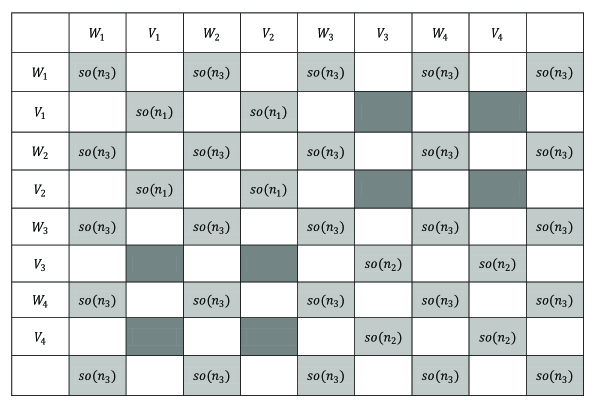
Figure 1: An illustration for the decomposition $\mathfrak{so}(9)=\mathfrak{so}(2)\oplus\mathfrak{so}(2)\oplus\mathfrak{so}(5)\oplus\mathfrak{v}$. We have $\mathfrak{v}=W_{1}\oplus\mathfrak{v}_{1}\oplus W_{2}\oplus\mathfrak{v}_{2}\oplus W_{3}\oplus\mathfrak{v}_{3}\oplus W_{4}\oplus\mathfrak{v}_{4}$, $\dim\mathfrak{v}_{1}=1$, $\dim\mathfrak{v}_{2}=2$, $\dim\mathfrak{v}_{3}=1$, and $\dim\mathfrak{v}_{4}=0$.

From the form of expressions of $P^{k}_{l}$ at the point $M_{0}$ and (11) it follows:

$$P^{k}_{l}(M_{0})\in W_{1}\oplus\dots\oplus W_{k},\qquad Q^{k}_{l}(M_{0})\in\mathfrak{v}_{1}\oplus\dots\oplus\mathfrak{v}_{k}.$$

Therefore,

$$U_{k}(M_{0})\subset\mathfrak{v}_{1}\oplus\mathfrak{v}_{2}\oplus\dots\oplus\mathfrak{v}_{k}.$$ (17)

For a collection of numbers $(n_{1},\dots,n_{r})$, $n_{1}\leq n_{2}\leq\dots\leq n_{r}$, $n_{r}\leq n_{1}+\dots+n_{r-1}+1$, in addition, we suppose the following assumption:

Assumption 1

There exists a permutation of diagonal elements of the matrix $A$, such that all $n_{i}$ elements equal to $\alpha_{i}$ are rearranged to occupy the places with indexes $j_{i},j_{i}+2,\dots,j_{i}+2(n_{i}-1)$, $i=1,2,\dots,r$. Here the index $j_{i}$ denotes the first appearance of an element equal to $\alpha_{i}$.

If the Assumption 1 is satisfied, then $\mathfrak{so}(n)_{A}$ is a subset of $V_{1}\oplus\dots\oplus V_{[n/2]}$, while the gradients $P^{k}_{l}(M_{0})$ belong to $W_{1}\oplus\dots\oplus W_{k}\subset\mathfrak{v}$. Therefore, $\operatorname{\mathrm{pr}}_{\mathfrak{so}(n)_{A}}P^{k}_{l}(M_{0})=0$ and $Q^{k}_{l}(M_{0})=[M_{0},P^{k}_{l}(M_{0})]$. Furthermore,

$$\dim\mathfrak{v}_{k}=\dim V_{k}-\delta_{k}=(n-2k)-\delta_{k},\qquad\delta_{k}=\dim\mathfrak{so}(n)_{A}\cap V_{k},$$

where

$$\delta_{k}=\delta_{k,1}+\dots+\delta_{k,r},\qquad\delta_{k,i}=\dim\mathfrak{so}(n_{i})\cap V_{k}$$

$$\delta_{k,i}=n_{i}-k,\quad k=1,\dots,n_{i}-1,\quad\delta_{k,i}=0,\quad k\geq n_{i}.$$

Example 1

If $n=9$, $r=3$ $n_{1}=2,n_{2}=2,n_{3}=5$, starting from

$$A=\operatorname{\mathrm{diag}}(\alpha_{1},\alpha_{1},\alpha_{2},\alpha_{2},\alpha_{3},\alpha_{3},\alpha_{3},\alpha_{3},\alpha_{3}),$$

a required permutation is (see Figure 1)

$$A=\operatorname{\mathrm{diag}}(\alpha_{3},\alpha_{1},\alpha_{3},\alpha_{1},\alpha_{3},\alpha_{2},\alpha_{3},\alpha_{2},\alpha_{3}).$$

On the other hand, the choice $r=3$, $n_{1}=n_{2}=n_{3}=3$ does not satisfy the Assumption 1. This is the only example for $n=9$, which does not satisfy the Assumption 1.

The components $S^{k}_{l,i}$ of the projection of $Q^{k}_{l}(M_{0})$ to $V_{k}$ can be easily calculated:

$$S^{1}_{1,i}=\langle Q^{1}_{1},E_{i}\wedge E_{i+2}\rangle=a_{i+2}-a_{i},$$

$$S^{1}_{2,i}=\langle Q^{1}_{2},E_{i}\wedge E_{i+2}\rangle=(a_{i+2}-a_{i})(a_{i}+a_{i+1}+a_{i+2}),$$

$$S^{1}_{3,i}=\langle Q^{1}_{3},E_{i}\wedge E_{i+2}\rangle=(a_{i+2}-a_{i})(a_{i}a_{i+1}+a_{i}a_{i+2}+a_{i+1}a_{i+2}+a_{i}^{2}+a_{i+1}^{2}+a_{i+2}^{2}),$$

$$\dots$$

$$S^{2}_{1,i}=\langle Q^{2}_{1},E_{i}\wedge E_{i+4}\rangle=a_{i+4}-a_{i},$$

$$S^{2}_{2,i}=\langle Q^{2}_{2},E_{i}\wedge E_{i+4}\rangle=(a_{i+4}-a_{i})(a_{i}+a_{i+1}+a_{i+2}+a_{i+3}+a_{i+4}),$$

$$S^{2}_{3,i}=\langle Q^{2}_{3},E_{i}\wedge E_{i+4}\rangle=(a_{i+4}-a_{i})\sum_{i\leq i_{1}\leq i_{i}\leq i+4}a_{i_{1}}a_{i_{2}},$$

$$\dots$$

$$S^{3}_{1,i}=\langle Q^{3}_{1},E_{i}\wedge E_{i+6}\rangle=a_{i+6}-a_{i},$$

$$S^{3}_{2,i}=\langle Q^{3}_{2},E_{i}\wedge E_{i+6}\rangle=(a_{i+6}-a_{i})(a_{i}+a_{i+1}+a_{i+2}+a_{i+3}+a_{i+4}+a_{i+5}+a_{i+6}),$$

$$S^{3}_{3,i}=\langle Q^{3}_{3},E_{i}\wedge E_{i+6}\rangle=(a_{i+6}-a_{i})\sum_{i\leq i_{1}\leq i_{i}\leq i+6}a_{i_{1}}a_{i_{2}},$$

$$\dots$$

Therefore, for any condition

$$a_{j_{i}}=a_{j_{i}+2}=a_{j_{i}+4}=\dots=a_{j_{i}+2(n_{i}-1)}=\alpha_{i},$$

$\delta_{k,i}$ columns $j_{i},j_{i}+2,j_{i}+4,\dots,j_{i}+2(n_{i}-k-1)$ of a $(n-2k)\times(n-2k)$-matrix $S^{k}$ are equal to zero

$$S^{k}_{1,j_{i}}=S^{k}_{2,j_{i}}=\dots=S^{k}_{n-2k,j_{i}}=0,$$

$$S^{k}_{1,j_{i}+2}=S^{k}_{2,j_{i}+2}=\dots=S^{k}_{n-2k,j_{i}+2}=0,$$

$$\dots$$

$$S^{k}_{1,j_{i}+2(n_{i}-k-1)}=S^{k}_{2,j_{i}+2(n_{i}-k-1)}=\dots=S^{k}_{n-2k,j_{i}+2(n_{i}-k-1)}=0.$$

Also, the non zero columns of $S^{k}$ are independent. Hence, the rank of $S^{k}$ is equal to $n-2k-\delta_{k}$ and

$$\operatorname{\mathrm{pr}}_{\mathfrak{v}_{k}}(U_{k}(M_{0}))=\mathfrak{v}_{k}.$$ (18)

Therefore, the relation (17) becomes an equality, and we obtain the condition (15):

$$\dim U(M_{0}) = \sum_{k=1}^{[n/2]}\dim V_{k}-\sum_{i=1}^{r}\sum_{k=1}^{n_{i}}(n_{i}-k)$$

$$= N_{\mathfrak{so}(n)}-[n/2]-\sum_{i=1}^{r}\dim\mathfrak{so}(n_{i})=N_{\mathfrak{v}}-[n/2].$$

Besides, as a bi-product, from the above analysis we get that

$$\mathcal{L}_{\mathfrak{v}}^{0}=\{p^{k}_{l}|_{\mathfrak{v}}\quad|\quad k=1,2,\dots,[n/2],\quad l=0,1,\dots,n-2k-\delta_{k}\}$$ (19)

is a complete set of independent integrals.

We verified directly that the polynomials (19) are independent even if the Assumption 1 does not hold in several cases. However, the proofs are not so elegant and we feel that in those cases, it is more natural to use a bi-Hamiltonian approach, as it was done by Mykytyuk [21].

Example 2

For the case considered in Example 1, the restrictions of

$$p^{1}_{0},\,p_{1}^{1},p^{2}_{0},\,p^{2}_{1},\,p^{2}_{2},\,p^{3}_{0},\,p^{3}_{1},\,p^{4}_{0}$$

to $\mathfrak{v}$ provide a complete commutative set on $\mathbb{R}[\mathfrak{v}]^{SO(2)\times SO(2)\times SO(5)}$.

2.2 Singular case

Next, we consider the case when

$$n_{r}=n_{1}+\dots+n_{r-1}+s,\qquad s>1.$$ (20)

Let $n^{\prime}=n-s$ and let $\mathfrak{so}(n^{\prime})=so(n^{\prime})_{A^{\prime}}\oplus\mathfrak{v}^{\prime}$ be the orthogonal decomposition, where $A^{\prime}$ is the $n^{\prime}\times n^{\prime}$-diagonal matrix obtained from $A$ by removing $s$ components equal to $\alpha_{r}$. Then

$$\mathfrak{so}(n^{\prime})_{A^{\prime}}\cong\mathfrak{so}(n_{1})\oplus\mathfrak{so}(n_{2})\oplus\dots\oplus\mathfrak{so}(n_{r-1})\oplus\mathfrak{so}(n_{r}-s),$$ (21)

and the condition (12) is satisfied for $\mathfrak{so}(n^{\prime})$ and $A^{\prime}$. Thus, if the Assumption 1 for $(n_{1},\dots,n_{r-1},n_{r}-s)$ is satisfied, the corresponding set $\mathcal{L}_{\mathfrak{v}^{\prime}}^{0}$ given by (19) is a complete commutative set on $\mathfrak{v}^{\prime}$. On the other hand, from the second part of the proof of Theorem 4 [8] we have

$$N_{\mathfrak{v}}=N_{\mathfrak{v}^{\prime}}.$$

Thus, the set of polynomials $\mathcal{L}_{\mathfrak{v}^{\prime}}^{0}$ is a complete commutative set of polynomials on $\mathfrak{v}$, where we instead the restrictions $p^{k}_{l}|_{\mathfrak{v}^{\prime}}$ we take the restrictions $p^{k}_{l}|_{\mathfrak{v}}$.

As a result, we proved the completeness of Manakov integrals for homogeneous spaces $SO(n)/SO(n_{1})\times\dots\times SO(n_{r})$, for collections of numbers $n_{1}\leq n_{2}\leq\dots\leq n_{r}$ described by

• $n_{r}\leq n_{1}+\dots+n_{r-1}+1$ and $(n_{1},\dots,n_{r})$ satisfy the Assumption 1;

• $n_{r}=n_{1}+\dots+n_{r-1}+s$, $s>1$ and $(n_{1},\dots,n_{r-1},n_{r}-s)$ satisfy the Assumption 1.

In particular, if all eigenvalues of $A$ are distinct then $\mathfrak{v}=\mathfrak{so}(n)$ and we obtain that all integrals $p^{k}_{l}$ are functionally independent. In that case, the above consideration can be considered as a simplified version of the Mishchenko–Fomenko theorem on the completeness of polynomials on normal subalgebras of complex semi-simple Lie algebras [23].

Acknowledgments

The research was supported by the Serbian Ministry of Science Project 174020 Geometry and Topology of Manifolds, Classical Mechanics, and Integrable Dynamical Systems. We are grateful to S. S. Nikolaenko for the correction of few misprints.

References

• [1]
• [2] Arnold, V. I.: Mathematical Methods of Classical Mechanics, Moskva, Nauka, 1974 (Russian). English translation: Springer 1988.
• [3] Bolsinov, A. V.: Compatible Poisson brackets on Lie algebras and the completeness of families of functions in involution, Izv. Acad. Nauk SSSR, Ser. matem. 55 (1991), no. 1, 68–92 (Russian). English translation: Math. USSR-Izv. 38 (1992), no.1, 69–90.
• [4] Bolsinov, A.V.: Complete commutative sets of polynomials in Poisson algebras: the proof of the Mishchenko-Fomenko conjecture. Tr. Sem. Vekt. Tenz. An. M.: Izd-vo MGU, (2005) 87–109 (Russian).
• [5] Bolsinov, A. V. and Jovanović, B.: Integrable geodesic flows on homogeneous spaces. Matem. Sbornik 192 (2001), no. 7, 21–40 (Russian). English translation: Sb. Mat. 192 (2001), no. 7-8, 951–969.
• [6] Bolsinov, A. V. and Jovanović, B.: Non-commutative integrability, moment map and geodesic flows. Annals of Global Analysis and Geometry 23 (2003), no. 4, 305-322, arXiv: math-ph/0109031.
• [7] Bolsinov, A. V. and Jovanović, B.: Complete involutive algebras of functions on cotangent bundles of homogeneous spaces. Mathematische Zeitschrift 246 (2004) no. 1-2, 213–236.
• [8] Dragović, V., Gajić B. and Jovanović, B.: Singular Manakov Flows and Geodesic Flows of Homogeneous Spaces of $SO(n)$, Transfomation Groups 14 (2009), no. 3, 513–530, arXiv:0901.2444.
• [9] Dragović, V., Gajić B. and Jovanović, B. Systems of Hess–Appelrot type and Zhukovskii property , International Journal of Geometric Methods in Modern Physics, 6 (2009), no. 8, 1253- 1304, arXiv:0912.1875.
• [10] Dikii, L. A., Hamiltonian systems connected with the rotation group, Funkc. Anal. Pril. 6 (1972), no. 4, 83–84 (Russian). English translation: Funct. Anal. Appl. 6 (1972) 326–327.
• [11] Dubrovin, B. A.: Finite-zone linear differential operators and Abelian varieties, Uspehi Mat. Nauk, 31 (1976), No. 4, 259–260 (Russian).
• [12] Dubrovin, B. A.: Completely integrable Hamiltonian systems connected with matrix operators and Abelian varieties, Funkc. Anal. Pril., 11 (1977), 28-41, (Russian).
• [13] Fedorov, Yu. N.: Integrable flows and Bc̈klund transformations on extended Stiefel varieties with application to the Euler top on the Lie group $SO(3)$, J. Non. Math. Phys. 12 (2005), Suppl. 2, 77–94.
• [14] Fedorov, Yu. N. and Kozlov, V. V.: Various aspects of $n$-dimensional rigid body dynamics, Amer. Math. Soc. Transl. Series 2, 168 141–171, 1995.
• [15] Frahm, F: Ueber gewisse Differentialgleichungen, Math. Ann. 8 (1874), 35–44.
• [16] Jovanović, B.: Integrability of Invariant Geodesic Flows on $n$-Symmetric Spaces, Annals of Global Analysis and Geometry, 38 (2010), 305–316, arXiv:1006.3693 [math.DG]
• [17] Jovanović, B.: Geodesic flows on Riemannian g.o. spaces, Regular and Chaotic Dynamics, 16 (2011), No. 5, 504–513, arXiv:1105.3651.
• [18] Manakov, S. V.: Note on the integrability of the Euler equations of $n$–dimensional rigid body dynamics, Funkc. Anal. Pril. 10 (1976), no. 4, 93–94 (Russian).
• [19] Mykytyuk, I. V.: Actions of Borel subgroups on homogeneous spaces of reductive complex Lie groups and integrability. Composito Math. 127 (2001), 55–67.
• [20] Mykytyuk, I. V. and Panasyuk A.: Bi-Poisson structures and integrability of geodesic flows on homogeneous spaces. Transformation Groups 9 (2004), no. 3, 289–308.
• [21] Mykytyuk, I. V.: Integrability of geodesic flows for metrics on suborbits of the adjoint orbits of compact groups, arXiv:1402.6526.
• [22] Mishchenko, A. S.: Integrals of geodesics flows on Lie groups, Funkts. Anal. Prilozh., 4 (1970), no. 3, 73 -77 (Russian).
• [23] Mishchenko, A. S. and Fomenko, A. T.: Euler equations on finite-dimensional Lie groups. Izv. Acad. Nauk SSSR, Ser. matem. 42 (1978), no. 2, 396–415 (Russian). English translation: Math. USSR-Izv. 12 (1978), no.2, 371–389.
• [24] Mishchenko, A. S. and Fomenko, A. T.: Generalized Liouville method of integration of Hamiltonian systems. Funkts. Anal. Prilozh. 12 (1978), no. 2, 46–56 (Russian). English translation: Funct. Anal. Appl. 12 (1978), 113–121.
• [25] Nekhoroshev, N. N.: Action-angle variables and their generalization. Tr. Mosk. Mat. O.-va. 26 (1972), 181–198, (Russian). English translation: Trans. Mosc. Math. Soc. 26 (1972), 180–198.
• [26] Sadetov, S. T.: A proof of the Mishchenko-Fomenko conjecture (1981). Dokl. Akad. Nauk 397 (2004), no. 6, 751–754(Russian).
• [27] Ratiu, T.: The motion of the free n-dimensional rigid body, Indiana U. Math. J. 29 (1980), 609 -627.
• [28] Thimm A.: Integrable geodesic flows on homogeneous spaces, Ergod. Th. & Dynam. Sys.,1 (1981), 495–517.
• [29] Trofimov, V. V. and Fomenko, A. T.: Algebra and geometry of integrable Hamiltonian differential equations. Moskva, Faktorial, 1995 (Russian).