Minimum time control of a pair of two-level quantum systems with opposite drifts

Abstract

In this paper we solve two equivalent time optimal control problems. On one hand, we design the control field to implement in minimum time the SWAP (or equivalent) operator on a two-level system, assuming that it interacts with an additional, uncontrollable, two-level system. On the other hand, we synthesize the SWAP operator simultaneously, in minimum time, on a pair of two-level systems subject to opposite drifts. We assume that it is possible to perform three independent control actions, and that the total control strength is bounded. These controls either affect the dynamics of the target system, under the first perspective, or, simultaneously, the dynamics of both systems, in the second view. We obtain our results by using techniques of geometric control theory on Lie groups. In particular, we apply the Pontryagin Maximum Principle, and provide a complete characterization of singular and non-singular extremals. Our analysis shows that the problem can be formulated as the motion of a material point in a central force, a well known system in classical mechanics. Although we focus on obtaining the SWAP operator, many of the ideas and techniques developed in this work apply to the time optimal implementation of an arbitrary unitary operator.

I Introduction

I.1 Statement of the problem

In this work we consider the controlled dynamics of a pair of interacting two-level quantum systems, where the purpose of the control action is the generation in minimum time of a desired unitary operation on one of these systems, which in the following will be called the target system ($T$). The other system represents an unavoidable disturbance or environment ($E$). The dynamics of the whole system is given by the Schrödinger operator equation

$$\dot{X}(t)=-iH(u)X(t),\qquad X(0)=I\otimes I,$$ (1)

where $X(t)$ describes the evolution of the density matrix of the composite system from its initial to its final configuration, $\rho(0)\rightarrow\rho(t)=X(t)\rho(0)X^{\dagger}(t)$, and $I$ is the identity operator for two-level systems. The initial state is assumed to be factorized, $\rho(0)=\rho_{E}(0)\otimes\rho_{T}(0)$, and $H(u)$ is the Hamiltonian of the system, given by

$$H(u)=I\otimes(u_{x}S_{x}+u_{y}S_{y}+u_{z}S_{z})+2\omega_{0}S_{z}\otimes S_{z}.$$ (2)

The first term in $H(u)$ contains three possibly time varying control actions $u_{k}=u_{k}(t)$, $k=x,y,z$, with $L_{2}$ norm bounded in strength, $u_{x}^{2}+u_{y}^{2}+u_{z}^{2}\leqslant\gamma^{2}$. These control actions are associated with the generators $S_{k}=\frac{1}{2}\sigma_{k}$, $k=x,y,z$, where $\sigma_{k}$ are the Pauli matrices

$$\sigma_{x}=\left(\begin{array}[]{cc}0&1\\ 1&0\\ \end{array}\right),\quad\sigma_{y}=\left(\begin{array}[]{cc}0&-i\\ i&0\\ \end{array}\right),\quad\sigma_{z}=\left(\begin{array}[]{cc}1&0\\ 0&-1\\ \end{array}\right),$$ (3)

with commuting relations $[\sigma_{k},\sigma_{l}]=2i\sigma_{m}$, and $(k,l,m)$ is a cyclic permutation of $(x,y,z)$. The second term in (2) represents an Ising interaction between the two systems; we assume $\omega_{0}\neq 0$, otherwise the problem reduces to that of controlling an isolated two-level system with bounded control, which has been solved in previous work AD ; RR . Without loss of generality we can take $\omega_{0}>0$, as we shall shortly see. We neglect the free evolution of the environmental two-level system. It is meant that terms on the right of the tensor product are associated to the target system. Because of the block structure of the Hamiltonian (2) and of the initial state $X(0)$, the evolution operator has a block structure at any time $t$,

$$X(t)={\rm diag}(X_{1}(t),X_{2}(t))=P_{1}\otimes X_{1}(t)+P_{2}\otimes X_{2}(t),$$ (4)

where the projectors $P_{1}$, $P_{2}$ are given by

$$P_{1}=\frac{1}{2}(I+\sigma_{z}),\qquad P_{2}=\frac{1}{2}(I-\sigma_{z}),$$ (5)

and the dynamics of the two blocks is given by

$$\dot{X}_{1}(t) = -i(\omega_{0}S_{z}+u_{x}S_{x}+u_{y}S_{y}+u_{z}S_{z})X_{1}(t),\quad X_{1}(0)=I,$$

$$\dot{X}_{2}(t) = -i(-\omega_{0}S_{z}+u_{x}S_{x}+u_{y}S_{y}+u_{z}S_{z})X_{2}(t),\quad X_{2}(0)=I.$$ (6)

The dynamics of the target system is obtained by taking the partial trace of $\rho(t)$ over the degrees of freedom of the environmental system; since ${\rm Tr}P_{i}P_{j}=\delta_{ij}$, we find

$$\rho_{T}(t)={\rm Tr}_{E}(\rho(t))={\rm Tr}_{E}\big{(}P_{1}\rho_{E}(0)\big{)}X_{1}(t)\rho_{T}(0)X_{1}^{\dagger}(t)+{\rm Tr}_{E}\big{(}P_{2}\rho_{E}(0)\big{)}X_{2}(t)\rho_{T}(0)X_{2}^{\dagger}(t).$$ (7)

Our task is to find the minimum time $t_{f}$ such that this evolution reproduces a given unitary operator $X_{f}\in SU(2)$ acting on the target system,

$$\rho_{T}(t_{f})=X_{f}\rho_{T}(0)X_{f}^{\dagger}.$$ (8)

In principle, the initial state of the environmental qubit $\rho_{E}(0)$ is unknown. Therefore, Eq.s (7) and (8) must hold for every $\rho_{E}(0)$. A necessary and sufficient condition for this is that $X_{1}(t_{f})=\pm X_{f}$ and $X_{2}(t_{f})=\pm X_{f}$, with all possible combinations of signs. In view of the evolution equations (I.1), we conclude that the problem of optimally steering a two-level system in interaction with a second two level system is equivalent to the problem of optimally driving two independent two-level systems, subject to opposite drifts, through the same control actions. Moreover, we see that our choice $\omega_{0}>0$ is not restrictive, since the case $\omega_{0}<0$ amounts to interchanging the two systems $1$ and $2$.

I.2 Motivation

The application to the study of quantum mechanical systems of methods of geometric control theory, and in particular optimal control theory, is a longstanding practice. These methods are particularly suitable in applications to the synthesis of specific operations in quantum information processing nielsen , the control of nuclear spins in nuclear magnetic resonance levitt , or the optimization of specific reactions in atomic or molecular physics.

In this context, two-level systems are often the building blocks of larger structures. Therefore, it is of great relevance to understand to what extent it is possible to manipulate them, especially when they are immersed in a dissipative environment (see wu ; boscain ; wenin ; carlini ; kirillova ; garon ; hegerfeldt ; aiello ; russell and references therein for some applications of optimal control theory to quantum systems). The standard approach for their control is given by dynamical decoupling techniques LidarReview , which, however, usually require unbounded control actions. Whenever a bound on the controls cannot be neglected, optimal control represents an alternative tool to dynamical decoupling.

A dissipative environment is usually modeled by a thermal bath with infinitely many degrees of freedom. However, for some specific systems, it is meaningful to model the external world by means of a finite-dimensional system. A noticeable example is provided by the study of NV centers in diamonds, which are currently of great interest for applications in quantum information technology (see, e.g. Slava1 ; Slava2 ). The control task is to drive a central spin independently of the environmental spins, whose coupling strengths to the central spin generally depend on their distances from it. The problem considered in this work is the simplest instance of this situation where only one environmental spin exists. See Burgarth for a numerical analysis of the dependence of the optimal time of transition on the number of environmental spins.

In all these scenarios it is desirable that a given state transfer occurs in minimum time. This is both to increase the efficiency of quantum operations which typically require a cascade of elementary gates and to minimize the effect of an (un-modeled) environment.

Besides applications in quantum mechanics, the optimal control of $SU(2)$ operations is strictly related to the optimal control on $SO(3)$, being $SU(2)$ the double cover of $SO(3)$. Since $SO(3)$ is the group modeling the attitude of a rigid body, our analysis is also of general interest in the study of classical mechanical systems.

I.3 Plan of the paper

We are able to derive analytical expressions for the time optimal control strategies, and the corresponding optimal times, for target operations equivalent to the SWAP operation, in the terms described in Proposition II.1, and for a specific range of values of $\omega_{0}$ and $\gamma$. Nonetheless, whenever appropriate, we present partial result valid for general target operations $X_{f}$.

In Section II we discuss the Lie algebraic structure of the problem, and briefly review the Pontryagin Maximum Principle (PMP) of optimal control theory pontryagin ; Flerish in the context of control on Lie groups. This fundamental result provides the theoretical framework for our investigation. The controls satisfying the PMP are candidate optimal and they are called extremals, and they are classified in nonsingular and singular extremals. Usually, the procedure for solving an optimal control problem by means of the PMP consists of several steps, which in our specific case are given by: (i) solution of the dynamical equations derived from the PMP; (ii) determination of the extremals; (iii) solution of the system dynamics for these control strategies, and computation of the corresponding time of transition to the desired target operator; (iv) determination of the optimal strategy by comparison of the different extremal strategies. In general, some of these steps cannot be carried out analytically, and one has to resort to numerical computations. In the present case, numerical analysis and the structure of the problem will suggest a conjecture, which, when adopted, allows an analytical result of the optimal control problem when $X_{f}=X_{SWAP}$.

We shall present a complete investigation of the aforementioned points (i) - (iv) for the system of interest here. This process is complicated by the presence of singular arcs, which require a separate analysis (see boscain2 ; wu2 ; lapert for applications of optimal control theory to quantum mechanical systems where singular solutions exist). In Section III we show that, in both cases of nonsingular and singular extremals, the basic equations derived by applying the PMP can be interpreted as the motion of a fictitious material point subject to a velocity-dependent force. If we choose the final target operator as $X_{f}=X_{SWAP}$, this force becomes conservative, and the system is equivalent to an integrable classical central force problem. This fact provides a parallel between this optimal control problem and the (deeply investigated) analysis of the motion of a material point in a central force broucke .

At this point, we find convenient to limit our attention to the case $X_{f}=X_{SWAP}$, and show that the extremal trajectories correspond to motions with null angular momentum in the effective central-force problem. This result is valid for both cases of nonsingular and singular extremals, which are separately investigated in Sections IV and V. A complete treatment of singular extremals can be performed for arbitrary values of $\gamma$ and $\omega_{0}$, but the investigation of nonsingular extremals is increasingly difficult as $\frac{\gamma}{\omega_{0}}$ decreases, therefore we limit our attention to cases where analytical solutions are possible. In Section VI, by comparing the different types of extremals previously found, we solve the optimal control problem for $X_{f}=X_{SWAP}$ in the aforementioned range of values of $\omega_{0}$ and $\gamma$, and provide the optimal control strategies and the optimal time. In Section VII we discuss our findings, relate them to existing results, and conclude.

For sake of clarity, the most technical results are reported in Appendices. Also, the most significant results, which are frequently referred to throughout the paper, are presented as Propositions, and formally proved. The reader not interested in the computational details could directly move to Section VI, where the main results are summarized. The investigation of cases other than $X_{f}=X_{SWAP}$ will be presented in a forthcoming paper, complementing the analysis presented here.

II The Lie algebraic structure of the problem

As anticipated in the Introduction, the optimal control problem that we consider in this work is the following: given the dynamical system (I.1) and a target operation $X_{f}\in SU(2)$, we want to find a control strategy $u_{k}(t)$, $k=x,y,z$, such that $X_{1}(t_{f})=\pm X_{f}$ and $X_{2}(t_{f})=\pm X_{1}(t_{f})$, and $t_{f}$ is minimum . First of all, we prove that, for every $\phi\in\mathbb{R}$, the operator

$$\hat{X}_{f}=e^{i\varphi S_{z}}X_{f}e^{-i\varphi S_{z}},$$ (9)

is reached in the same optimal time as $X_{f}$.

Proposition II.1.

Consider a pair of operators $X_{f}$ and $\hat{X}_{f}\in SU(2)$ which satisfy (9) for some $\varphi$. Assume that there is a control strategy $u_{k}=u_{k}(t)$ ($k=x,y,z$), with $u_{x}^{2}+u_{y}^{2}+u_{z}^{2}\leqslant\gamma^{2}$, such that $X_{1}$ and $X_{2}$ are mapped to $X_{f}$ (or its negative) in time $t_{f}$. Then there is a control strategy $\hat{u}_{k}=\hat{u}_{k}(t)$ ($k=x,y,z$), with $\hat{u}_{x}^{2}+\hat{u}_{y}^{2}+\hat{u}_{z}^{2}\leqslant\gamma^{2}$, such that $X_{1}$ and $X_{2}$ are mapped to $\hat{X}_{f}$ (or its negative) in the same time $t_{f}$.

Proof: If we define $\hat{X}_{1}=e^{i\varphi S_{z}}X_{1}e^{-i\varphi S_{z}}$ and $\hat{X}_{2}=e^{i\varphi S_{z}}X_{2}e^{-i\varphi S_{z}}$, we can write

$$\dot{\hat{X}}_{1}(t) = -i(\omega_{0}S_{z}+\hat{u}_{x}S_{x}+\hat{u}_{y}S_{y}+\hat{u}_{z}S_{z})\hat{X}_{1}(t),\quad\hat{X}_{1}(0)=I,$$

$$\dot{\hat{X}}_{2}(t) = -i(-\omega_{0}S_{z}+\hat{u}_{x}S_{x}+\hat{u}_{y}S_{y}+\hat{u}_{z}S_{z})\hat{X}_{2}(t),\quad\hat{X}_{2}(0)=I,$$ (10)

where $\hat{u}_{x}=u_{x}\cos{\varphi}+u_{y}\sin{\varphi}$, $\hat{u}_{y}=-u_{x}\sin{\varphi}+u_{y}\cos{\varphi}$, and $\hat{u}_{z}=u_{z}$. These controls satisfy the required constraint since $u_{x}^{2}+u_{y}^{2}+u_{z}^{2}=\hat{u}_{x}^{2}+\hat{u}_{y}^{2}+\hat{u}_{z}^{2}$, therefore they represent an admissible control strategy. Moreover, the dynamics (II) is formally the same as (I.1), therefore the control strategy $\hat{u}_{k}=\hat{u}_{k}(t)$ generates the desired transformation $X_{1}(t_{f})=\pm X_{f}$ and $X_{2}(t_{f})=\pm X_{1}(t_{f})$.

This result is a consequence of a symmetry of the problem, defined by the transformations $\hat{\sigma}_{k}=e^{i\varphi S_{z}}\sigma_{k}e^{-i\varphi S_{z}}$ for $k=x,y$, and $\hat{\sigma}_{z}=\sigma_{z}$. This change of representation of the Pauli matrices does not affect the system, since it merely corresponds to a redefinition of the controls, but it leaves invariant the equations of motion (I.1). The particular form of the controls in the dynamics is crucial for the existence of this symmetry, which is preserved even if there are only two independent controls affecting $\sigma_{x}$ and $\sigma_{y}$ (that is, $u_{z}\equiv 0$).

Following Proposition II.1, we will consider equivalent two target operators which satisfy (9) for some $\varphi$. Therefore, it is sufficient to solve the optimal control problem for one of them to obtain a complete description of the optimal control strategies and optimal time for all of them. We will rely on this fact, when we will fully solve the case with $X_{f}=X_{SWAP}$ (or equivalent operators). In the representation induced by (3), operators related by (9) differ by a phase in the off diagonal terms.

It is well known in quantum control theory miko that information on the structure of a control problem can be obtained by analyzing the Lie algebra associated to the system. We define the block-diagonal matrices:

$$B_{k}=\left(\begin{array}[]{cc}S_{k}&0\\ 0&S_{k}\\ \end{array}\right),\qquad C_{k}=\left(\begin{array}[]{cc}S_{k}&0\\ 0&-S_{k}\\ \end{array}\right),$$ (11)

where $S_{k}=\frac{1}{2}\sigma_{k}$, and $0$ is the $2\times 2$ null matrix, and $k=x,y,z$. In terms of them, the evolution (1) takes the form

$$\dot{X}(t)=-i(\omega_{0}C_{z}+u_{x}B_{x}+u_{y}B_{y}+u_{z}B_{z})X(t),\quad X(0)=I\otimes I.$$ (12)

Since we want to find the controls steering in minimum time $t_{f}$ the evolution operator to $X(t_{f})={\rm diag}(X_{f},X_{f})$, or $X(t_{f})={\rm diag}(X_{f},-X_{f})$, or their negatives, where $X_{f}\in SU(2)$, we first apply results on the controllability of the system, to answer the question of whether this type of state transfer is possible. This is indeed the case since the Lie algebra generated by the Hamiltonians $C_{z}$, $B_{x}$, $B_{y}$ and $B_{z}$ in (12) is, in the considered representation, the Lie algebra of block diagonal $4\times 4$ matrices with arbitrary $2\times 2$ blocks in $\mathfrak{su}(2)$. The set of reachable operators is the associated Lie group of block diagonal $4\times 4$ matrices with $2\times 2$ blocks in $SU(2)$. This group contains the desired final conditions for any special unitary operator $X_{f}$. Therefore, system (12) is controllable on the Lie group of operators of the form ${\rm diag}(Y,Z)$, where $Y,Z\in SU(2)$. This group is compact, semisimple, and isomorphic to $SU(2)\oplus SU(2)$. The associated Lie algebra, isomorphic to $\mathfrak{su}(2)\oplus\mathfrak{su}(2)$, is given by $\mathfrak{l}=\mathfrak{b}\oplus\mathfrak{c}$, where

$$\mathfrak{b}={\rm span}(B_{x},B_{y},B_{z}),\qquad\mathfrak{c}={\rm span}(C_{x},C_{y},C_{z})$$ (13)

satisfy the commutation relations of a Cartan decomposition of $\mathfrak{l}$,

$$[\mathfrak{b},\mathfrak{b}]\subseteq\mathfrak{b},\quad[\mathfrak{c},\mathfrak{c}]\subseteq\mathfrak{b},\quad[\mathfrak{b},\mathfrak{c}]\subseteq\mathfrak{c}.$$ (14)

More specifically, the commutation relations of the operators in (11) are given by

$$[B_{k},B_{l}]=iB_{m},\quad[C_{k},C_{l}]=iB_{m},\quad[B_{k},C_{l}]=iC_{m},$$ (15)

and $(k,l,m)$ is a cyclic permutation of $(x,y,z)$. The controllability properties of the system along with the fact that the set of possible values for the control is compact allows us to use the standard Filippov’s existence result for time optimal control problems (see, e.g., Flerish ) to conclude that the time optimal control exists for every final condition in $SU(2)\oplus SU(2)$ .

To solve our problem, we shall apply the classical necessary conditions of optimality given by the Pontryagin Maximum Principle (see, e.g., Flerish and miko2 ; Tesi for application to quantum systems on Lie groups). In order to state them in a form appropriate for our goals, we set up some definitions. Given $M\in\mathfrak{l}$ (usually called the costate), and $X$ a solution of (12), we define the time-dependent coefficients

$$b_{k}=i\langle M,X^{\dagger}B_{k}X\rangle,\quad c_{k}=i\langle M,X^{\dagger}C_{k}X\rangle,$$ (16)

where $\langle A,B\rangle={\rm Tr}(AB^{\dagger})$, and $k=x,y,z$.

Definition 1.

The Pontryagin Hamiltonian is defined as

$$H(M,X,v_{x},v_{y},v_{z})=\omega_{0}c_{z}+\sum_{k=x,y,z}v_{k}b_{k}.$$ (17)

Theorem 1.

- Pontryagin Maximum Principle (PMP) - Assume that the evolution of $X$ is described by (12), and that $u_{x},u_{y},u_{z}$ is the time optimal control strategy steering $X$ from the identity $I\otimes I$ to ${\rm diag}(X_{f},X_{f})$ or ${\rm diag}(X_{f},-X_{f})$. Denote by $\tilde{X}(t)$ the corresponding trajectory. Then there exists an operator $\tilde{M}\in\mathfrak{l}$, $\tilde{M}\neq 0$, a constant $\lambda$, and functions $b_{k}$, $c_{k}$ as in (16), such that $H(\tilde{M},\tilde{X},u_{x},u_{y},u_{z})\geqslant H(\tilde{M},\tilde{X},v_{x},v_{y},v_{z})$ for every $v_{x}$, $v_{y}$, $v_{z}$ such that $v_{x}^{2}+v_{y}^{2}+v_{z}^{2}\leqslant\gamma^{2}$. Moreover, the Pontryagin Hamiltonian is constant and equal to $\lambda$.

Controls satisfying the conditions of Theorem 1 are called extremals, and they are candidate optimal controls, since the PMP is a necessary condition for optimality. They are called normal extremals if $\lambda\neq 0$, abnormal otherwise. The arcs of the extremal trajectories where the Pontryagin Hamiltonian does not explicitly depend on the controls are called singular, and in this specific case they are described by $b_{x}\equiv b_{y}\equiv b_{z}\equiv 0$. In general an extremal trajectory can contain both singular and nonsingular arcs. We shall call singular a trajectory which contains at least one singular arc, nonsingular otherwise.

The procedure to find the time optimal control consists of computing all the extremals, and then compare the values of the time needed to reach the desired final condition and choose the control which gives the minimum time.

For both singular and nonsingular arcs, and, in fact, for every control, the functions defined in (16) satisfy the following differential equations,

$$\dot{b}_{x} = -\omega_{0}c_{y}-u_{z}b_{y}+u_{y}b_{z},$$

$$\dot{b}_{y} = \omega_{0}c_{x}+u_{z}b_{x}-u_{x}b_{z},$$

$$\dot{b}_{z} = u_{x}b_{y}-u_{y}b_{x},$$

$$\dot{c}_{x} = -\omega_{0}b_{y}+u_{y}c_{z}-u_{z}c_{y},$$

$$\dot{c}_{y} = \omega_{0}b_{x}-u_{x}c_{z}+u_{z}c_{x},$$

$$\dot{c}_{z} = u_{x}c_{y}-u_{y}c_{x}.$$ (18)

They can be derived by differentiating (16), taking into account the evolution (12), and the commuting relations (15).

For some given initial conditions $b_{k}(0)$, and $c_{k}(0)$, $k=x,y,z$ the final conditions $b_{k}(t_{f})$ and $c_{k}(t_{f})$, are obtained by taking $X_{f}=X(t_{f})$ in (16). They read

$$b_{k}(t_{f})=\sum_{l}\mathcal{X}_{kl}b_{l}(0),\qquad c_{k}(t_{f})=\sum_{l}\mathcal{X}_{kl}c_{l}(0),$$ (19)

where $\mathcal{X}\in SO(3)$ is a matrix representation of the element associated with $X_{f}$. This follows from the fact that $SU(2)$ is the double covering group of $SO(3)$.

It turns out that (17) is not the only constant of motion on extremal trajectories.

Proposition II.2.

System (II) admits the following integrals of motion :

$$E=\frac{\omega^{2}_{0}}{2}\sum_{k=x,y,z}(b_{k}^{2}+c_{k}^{2}),\qquad L=\omega_{0}\sum_{k=x,y,z}b_{k}c_{k}.$$ (20)

Proof: The fact that $\dot{E}=\dot{L}=0$ is a direct consequence of (II).

In the next section we will provide a useful interpretation of these constants. To complete this section, we derive some results which will be needed in the following. First of all, we characterize the structure of extremal control strategies. On nonsingular arcs, since the Pontryagin Hamiltonian is linear in $v_{x}$, $v_{y}$ and $v_{z}$, its maximum in the set $v_{x}^{2}+v_{y}^{2}+v_{z}^{2}\leqslant\gamma^{2}$ must be on the border of this set. By applying the Lagrange multipliers method we find that the extremal controls satisfy

$$u_{k}=\gamma\frac{b_{k}}{\mu_{b}},\qquad k=x,y,z$$ (21)

where $\mu_{b}=\sqrt{b_{x}^{2}+b_{y}^{2}+b_{z}^{2}}$. On nonsingular arcs, $\mu_{b}$ can vanish only in isolated points. From standard theorems on ordinary differential equations, it follows that $b_{k}$ must be continuous, and then the controls $u_{k}$ must be piecewise continuous.

Remark II.3.

At the beginning of this section, we have proved that two target operators $X_{f}$ and $\hat{X}_{f}$ satisfying (9) are reached in the same minimum time. One possible interpretation of this result is to think of (9) as a symmetry transformation which preserves the Lie algebraic structure of the problem. Accordingly, if the matrix $M\in\mathfrak{l}$ appearing in the PMP is associated with $X_{f}$, the corresponding operator $\hat{M}\in\mathfrak{l}$ associated with $\hat{X}_{f}$, must be given by

$$\hat{M}=e^{i\varphi S_{z}}Me^{-i\varphi S_{z}},\qquad\varphi\in\mathbb{R}.$$ (22)

The coefficients (16) are transformed as $\hat{b}_{x}=b_{x}\cos{\varphi}+b_{y}\sin{\varphi}$, $\hat{b}_{y}=-b_{x}\sin{\varphi}+b_{y}\cos{\varphi}$ and $\hat{b}_{z}=b_{z}$, where $\hat{b}_{k}$, $k=x,y,z$, are associated with $\hat{M}$ (the same transformation describes the map of the $c_{k}$ coefficients into $\hat{c}_{k}$), and the Pontryagin Hamiltonian is unchanged.

III The costate dynamics as a central-force problem

In this section we reinterpret the costate dynamics, i.e. Eq.s (II), as a central-force problem. This parallel provides a useful bridge between our problem and a well know scenario in classical mechanics, which has been deeply investigated in the past. While we will find this connection especially useful in the special case $X_{f}=X_{SWAP}$ or equivalent operator, we believe that it is significant for more general final conditions. Therefore, for sake of completeness, initially we consider a generic target operator, and then we specialize our analysis to the case-study of $X_{f}=X_{SWAP}$.

Assume we are on a nonsingular extremals. By using the general form of the controls (21), we see from (II) that $\dot{b}_{z}\equiv 0$, and then $b_{z}=b_{z}(0)$ is a constant. This implies that

$$\dot{\mu}_{b}=\frac{1}{\mu_{b}}(b_{x}\dot{b}_{x}+b_{y}\dot{b}_{y})=-\frac{\omega_{0}}{\gamma}\dot{c}_{z},$$ (23)

which is equivalent to the constancy of the Pontryagin Hamiltonian on nonsingular extremals:

$$H(\tilde{M},\tilde{X},u_{x},u_{y},u_{z})=\lambda=\omega_{0}c_{z}+\gamma\mu_{b}=\omega_{0}c_{z}(0)+\gamma\mu_{b}(0).$$ (24)

This result is embodied in the last equation in (II). The other equations reduce to

$$\dot{b}_{x} = -\omega_{0}c_{y},$$

$$\dot{b}_{y} = \omega_{0}c_{x},$$

$$\dot{c}_{x} = -\omega_{0}b_{y}+\frac{\gamma}{\mu_{b}}\big{(}b_{y}c_{z}-b_{z}(0)c_{y}\big{)},$$

$$\dot{c}_{y} = \omega_{0}b_{x}-\frac{\gamma}{\mu_{b}}\big{(}b_{x}c_{z}-b_{z}(0)c_{x}\big{)},$$ (25)

which, on account of (24), can be written as

$$\ddot{b}_{x} = -(\omega_{0}^{2}+\gamma^{2})b_{x}+\gamma\lambda\frac{b_{x}}{\mu_{b}}-\gamma b_{z}(0)\frac{\dot{b}_{y}}{\mu_{b}}$$

$$\ddot{b}_{y} = -(\omega_{0}^{2}+\gamma^{2})b_{y}+\gamma\lambda\frac{b_{y}}{\mu_{b}}+\gamma b_{z}(0)\frac{\dot{b}_{x}}{\mu_{b}}$$ (26)

These non-linear equations can be interpreted as modeling the motion of a material point of unit mass, described by a “position” vector ${\bf b}=(b_{x},b_{y})=(b\cos{\theta},b\sin{\theta})$, in Cartesian or polar coordinates, respectively. This point is driven by a central force, the first and second terms in the right hand side of (III), plus a term dependent on “velocity” (the last contribution in both equations). By using a compact notation,

$$\ddot{{\bf b}}={\bf F}({\bf b})+{\bf f}({\bf b},\dot{{\bf b}}),$$ (27)

where

$${\bf F}({\bf b})=-(\omega_{0}^{2}+\gamma^{2}){\bf b}+\gamma\lambda\frac{{\bf b}}{\sqrt{b^{2}+b_{z}^{2}(0)}},\quad{\bf f}({\bf b},\dot{{\bf b}})=-i\gamma b_{z}(0)\sigma_{y}\frac{\dot{{\bf b}}}{\sqrt{b^{2}+b_{z}^{2}(0)}}.$$ (28)

The velocity-dependent term is not a dissipative contribution. In fact, it is possible to interpret the integral of motion $E$ of the system, given in Proposition II.2, as the associated energy. This can be seen by introducing the potential associated to the radial part of the force,

$$U(b)=\frac{1}{2}(\omega_{0}^{2}+\gamma^{2})\left(b^{2}+b_{z}^{2}(0)\right)-\gamma\lambda\sqrt{b^{2}+b_{z}^{2}(0)}+\frac{1}{2}\lambda^{2},$$ (29)

with ${\bf F}({\bf b})=-{\rm grad}_{\bf b}U(b)$. It follows that

$$E=U(b)+\frac{1}{2}\Big{(}\dot{b}^{2}+(b\dot{\theta})^{2}\Big{)},$$ (30)

which justifies the interpretation of $E$ as the energy (potential plus kinetic energy). The energy is conserved, and there is no dissipation.

Since we have found $b_{z}\equiv b_{z}(0)$, and by virtue of (19), we can conclude that $b(t_{f})=b(0)$. Since $E$ is an integral of motion, we must also have $c_{z}(t_{f})=c_{z}(0)$ (alternatively, this is a consequence of the invariance of the Pontryagin Hamiltonian).

III.1 The case $X_{f}=X_{SWAP}$

If we assume $X_{f}=X_{SWAP}$ or any equivalent operator parameterized by $\varphi$ according to Proposition II.1, we have some simplifications. Therefore, here and in the following sections we will limit our attention to this special case, and then comment about the general case again in Section VII. Since we consider special unitary target operators, we conventionally write $X_{SWAP}=i\sigma_{y}$, and then the aforementioned family of equivalent operators is given by

$$X_{f}=\left(\begin{array}[]{cc}0&e^{i\varphi}\\ -e^{-i\varphi}&0\\ \end{array}\right),$$ (31)

where $\varphi$ is an arbitrary real number, which can be taken in the interval $[0,2\pi)$ without loss of generality. The $SO(3)$ matrix introduced in (19) is given by

$$\mathcal{X}=\left(\begin{array}[]{ccc}-\cos{2\varphi}&\sin{2\varphi}&0\\ \sin{2\varphi}&\cos{2\varphi}&0\\ 0&0&-1\\ \end{array}\right),$$ (32)

which is a rotation of angle $\pi$ about the axis defined by the unit vector $(\sin{\varphi},\cos{\varphi},0)$. For the final coordinates we must have

$$b_{x}(t_{f}) = -b_{x}(0)\cos{2\varphi}+b_{y}(0)\sin{2\varphi},$$

$$b_{y}(t_{f}) = b_{x}(0)\sin{2\varphi}+b_{y}(0)\cos{2\varphi},$$

$$b_{z}(t_{f}) = -b_{z}(0),$$ (33)

or, in polar coordinates, $b(t_{f})=b(0)$ (as we already know), and $\theta(t_{f})=\pi-\theta(0)-2\varphi$. Similar relations hold for $c_{k}(t_{f})$. Consistency with the former constraints requires $b_{z}(t_{f})=b_{z}(0)=0$ and $c_{z}(t_{f})=c_{z}(0)=0$. This implies that the Pontryagin Hamiltonian equals $\lambda=\gamma b(0)$, the velocity-dependent term disappears, ${\bf f}({\bf b},\dot{{\bf b}})={\bf 0}$, and the central force simplifies to

$${\bf F}({\bf b})=-(\omega_{0}^{2}+\gamma^{2}){\bf b}+\gamma\lambda\frac{{\bf b}}{b}.$$ (34)

The associated potential is given by

$$U(b)=\frac{1}{2}(\omega_{0}^{2}+\gamma^{2})b^{2}-\gamma\lambda b,$$ (35)

which belongs to the class of integrable potentials, with solutions given in terms of elliptic integrals. Initial and final positions and velocities are related by an orthogonal transformation, the upper $2\times 2$ diagonal block in (32). Moreover, the integral of motion $L$, given in Proposition II.2, takes the form

$$L=b^{2}\dot{\theta},$$ (36)

and then it can be interpreted as the angular momentum of the system.

Because of its particular simplicity, which highly limits the need of numerical analysis, in the reminder of this paper we will fully explore this case. As anticipated in the Introduction, we now separately consider nonsingular and singular extremals.

IV Nonsingular extremals for $\rm X_{f}=X_{SWAP}$

In this section we limit our attention to nonsingular extremals, for which $\mu_{b}$ can vanish only at isolated points. Following the analysis of the previous section, we know that it is possible to express the costate dynamics in terms of elliptic integrals. Unfortunately, this is not enough to provide useful expressions for the integrals of (I.1), that is, suitable expressions for the comparison of the extremal trajectories. Nonetheless, numerical computations suggests that the minimum time trajectories are characterized by $L=0$. We are not able to prove this result analytically, but we have found numerical evidence of its validity. We refer to Appendix A for more details on the numerical analysis supporting this fact.

Conjecture 1.

If $X_{f}=X_{SWAP}$, and an extremal control strategy is optimal, then the corresponding trajectory satisfies $L=0$.

Under this assumption, the dynamics of the costate greatly simplifies, and it is possible to compute explicit expressions for the evolution in the Lie group.

The following argument is based on Proposition II.3. If we assume that the optimal control strategy leading to $X_{f}=X_{SWAP}$ requires ${\mathbf{b}}(0)=(b_{x}(0),b_{y}(0))$, then an equivalent operator, differing from $X_{f}$ by a phase $\varphi$ in the off-diagonal elements, is associated with the counter-clockwise rotation by an angle $\varphi$ of ${\mathbf{b}}(0)$. In particular, one of these operators has to be associated with ${\mathbf{b}}(0)=(b_{x}(0),0)$, with $b_{x}(0)\geqslant 0$. According to Proposition II.1, there is no loss of generality in choosing this operator as $X_{f}$: the general analysis of any operator equivalent to SWAP will follow .

Since we have assumed $L=0$, we can write ${\mathbf{b}}(t)=(b_{x}(t),0)$, and then $b_{y}(t)\equiv 0$, which implies $b_{y}(t_{f})=0$. But validity of (III.1) imposes that $\sin{2\varphi}=0$, which can be satisfied either by $\varphi=0$ or $\varphi=\frac{\pi}{2}$. These two cases correspond to $X_{f}=i\sigma_{y}$ and $X_{f}=i\sigma_{x}$, respectively. Before analyzing them, we determine the structure of extremal control strategies for nonsingular arcs.

Since $\mu_{b}=|b_{x}|$, we can rewrite the first equation in (III) as

$$\ddot{b}_{x}=-(\omega_{0}^{2}+\gamma^{2})b_{x}+{\rm sign}(b_{x})\gamma^{2}b_{x}(0),$$ (37)

with general solution

$$b_{x}(t)=A_{j}\cos{\omega t}+B_{j}\sin{\omega t}+{\rm sign}(b_{x})\left(\frac{\gamma}{\omega}\right)^{2}b_{x}(0),$$ (38)

where $\omega^{2}=\omega_{0}^{2}+\gamma^{2}$. The coefficients $A_{j}$ and $B_{j}$, $j=0,1,2,\ldots$ are determined by the initial conditions, and by the requirement that $b_{x}(t)$ and $\dot{b}_{x}(t)$ are continuous functions (whenever $b_{x}$ vanishes, new coefficients must be taken into account). The initial pair of coefficients is given by

$$A_{0}=\left(\frac{\omega_{0}}{\omega}\right)^{2}b_{x}(0),\qquad B_{0}=\pm\frac{\omega_{0}}{\omega}\sqrt{1-b_{x}(0)^{2}},$$ (39)

and $B_{0}$ has been written under the assumption that $E=\frac{\omega^{2}_{0}}{2}$, since the value of this constant does not affect the optimal control problem. The sign of $B_{0}$ is the same as the sign of $\dot{b}_{x}(0)$. We have two possible solutions (38), depending on the sign of $B_{0}$. All the other coefficients $A_{j}$ and $B_{j}$ are completely determined by the continuity requirements, and their explicit expressions are not needed for further developments. Following (21), the optimal control strategy is necessarily bang-bang, with

$$u_{x}=\gamma\,{\rm sign}(b_{x}),\qquad u_{y}=u_{z}=0.$$ (40)

If they exist, the switching times are given by the zeros of (38), which depend on $b_{x}(0)$. We denote these switching times by $\tilde{t}_{k}=\tilde{t}+k\bar{t}$, $k=0,1,2,\ldots$, with $\bar{t}\geqslant\tilde{t}\geqslant 0$. The zeros of (38) satisfy

$$\cos{\omega t_{\pm}} = \frac{-A_{0}C_{0}\pm B_{0}\sqrt{A_{0}^{2}+B_{0}^{2}-C_{0}^{2}}}{A_{0}^{2}+B_{0}^{2}},$$

$$\sin{\omega t_{\pm}} = \frac{-B_{0}C_{0}\mp A_{0}\sqrt{A_{0}^{2}+B_{0}^{2}-C_{0}^{2}}}{A_{0}^{2}+B_{0}^{2}},$$ (41)

with $A_{0}$ and $B_{0}$ as in (39), and $C_{0}=\left(\frac{\gamma}{\omega}\right)^{2}b_{x}(0)$. We can assume that $t_{+}$ and $t_{-}$ are, in absolute value, the smaller and next to smaller zeros, not necessarily in this order. If $b_{x}(0)\neq 0$, by considering both positive or negative values for $B_{0}$ in (IV), we find that $\sin{\omega t_{+}}\leqslant\sin{\omega t_{-}}$. Moreover, for $B_{0}\geqslant 0$ we find $\cos{\omega t_{+}}\geqslant\cos{\omega t_{-}}$, $\cos{\omega t_{-}}\leqslant 0$ and $\sin{\omega t_{+}}\leqslant 0$, and for $B_{0}<0$, we find $\cos{\omega t_{+}}\leqslant\cos{\omega t_{-}}$, $\cos{\omega t_{+}}\leqslant 0$ and $\sin{\omega t_{-}}\geqslant 0$. From these properties we can conclude that, in any case, $t_{-}\geqslant 0$ and $t_{+}\leqslant 0$, so that

$$\cos{\omega\tilde{t}}=\cos{\omega t_{-}},\qquad\sin{\omega\tilde{t}}=\sin{\omega t_{-}}$$ (42)

and $\bar{t}=(t_{-}-t_{+})$, leading to

$$\cos{\omega\bar{t}}=\frac{2C_{0}^{2}-A_{0}^{2}-B_{0}^{2}}{A_{0}^{2}+B_{0}^{2}},\qquad\sin{\omega\bar{t}}=-\frac{2C_{0}\sqrt{A_{0}^{2}+B_{0}^{2}-C_{0}^{2}}}{A_{0}^{2}+B_{0}^{2}}.$$ (43)

We don’t need explicit expressions of $\tilde{t}$ and $\bar{t}$ in terms of $\omega_{0}$, $\gamma$ and $b_{x}(0)$, and Eq.s (43), (42) and (IV) will be sufficient to fully specify the control strategies in the case of interest for this work. In the special case $b_{x}(0)=0$, we have $A_{0}=C_{0}=0$ and $B_{0}=\pm\frac{\omega_{0}}{\omega}$, from which we can evaluate $\tilde{t}=\bar{t}=\frac{\pi}{\omega}$. For further reference, we observe the following:

Proposition IV.1.

From $\sin{\omega\bar{t}}\leqslant 0$ we have that $\frac{\pi}{\omega}\leqslant\bar{t}\leqslant\frac{2\pi}{\omega}$. Moreover, $0\leqslant\tilde{t}\leqslant\frac{\pi}{\omega}$.

In the following, we separately consider the two aforementioned cases $X_{f}=i\sigma_{y}$ or $X_{f}=i\sigma_{x}$.

IV.1 Case with $X_{f}=i\sigma_{y}$

By using $\varphi=0$ in (III.1), we derive the final condition $b_{x}(t_{f})=-b_{x}(0)$. An explicit computation proves that, if $b_{x}(0)=0$ and the control $u_{x}$ is constant, it is impossible to reproduce $X_{f}$. Therefore, control strategies associated with these nonsingular extremals have an odd number of switching times. We adopt the following definitions:

$$S_{+}=\frac{1}{\omega}(\gamma S_{x}+\omega_{0}S_{z}),\qquad S_{-}=\frac{1}{\omega}(\gamma S_{x}-\omega_{0}S_{z}),$$ (44)

and with $\omega=\sqrt{\omega_{0}^{2}+\gamma^{2}}$. By integrating the dynamics (I.1), we find

$$X_{1}(t) = Y^{\dagger}_{-}(\tilde{t})\Big{(}Y_{+}(\bar{t})Y^{\dagger}_{-}(\bar{t})\Big{)}^{n}Y_{+}(\tilde{t}),$$

$$X_{2}(t) = Y^{\dagger}_{+}(\tilde{t})\Big{(}Y_{-}(\bar{t})Y^{\dagger}_{+}(\bar{t})\Big{)}^{n}Y_{-}(\tilde{t}),$$ (45)

where $n=0,1,2,\ldots$, and we have used the notation

$$Y_{+}(t)=e^{-i\omega tS_{+}},\qquad Y_{-}(t)=e^{-i\omega tS_{-}}.$$ (46)

By requiring that $X_{1}(t_{f})=-X_{2}(t_{f})=\pm X_{f}$, from the pair of equations (IV.1), we obtain

$$\Big{(}Y_{+}(\bar{t})Y^{\dagger}_{-}(\bar{t})\Big{)}^{n}=\pm Y_{-}(\tilde{t})X_{f}Y^{\dagger}_{+}(\tilde{t}),$$ (47)

and the total time of evolution on these nonsingular trajectories is $t_{f}=2(\tilde{t}+n\bar{t})$. It turns out that the other possibility, $X_{1}(t_{f})=X_{2}(t_{f})=\pm X_{f}$, is inconsistent. To compactly present the treatment of this case, we find convenient to define two functions $\alpha=\alpha(\omega_{0},\gamma,\bar{t})$ and $\beta=\beta(\omega_{0},\gamma,\bar{t})$ satisfying

$$\sin{\alpha}=\left(\frac{\omega_{0}}{\omega}\right)\sin{\omega\bar{\tau}}, \cos{\alpha}=\sqrt{1-\left(\frac{\omega_{0}}{\omega}\right)^{2}\sin^{2}{\omega\bar{\tau}}},$$

$$\sin{\beta}=-\sec{\alpha}\cos{\omega\bar{\tau}}, \cos{\beta}=\frac{\gamma}{\omega}\sec{\alpha}\sin{\omega\bar{\tau}},$$ (48)

where $\bar{\tau}=\frac{\bar{t}}{2}$. These definitions are meaningful only when $\cos{\alpha}\neq 0$, which is always the case if $\gamma\neq 0$. To prove that they are consistent is a lengthy but standard problem of trigonometry. We can now write in compact form

$$Y_{+}(\bar{t})Y^{\dagger}_{-}(\bar{t})=\cos{2\alpha}I+i\sin{2\alpha}\,(\cos{\beta}\sigma_{y}+\sin{\beta}\sigma_{z}),$$ (49)

from which it follows that we can express the left-hand side of (47) as

$$\Big{(}Y_{+}(\bar{t})Y^{\dagger}_{-}(\bar{t})\Big{)}^{n}=\cos{2n\alpha}I+i\sin{2n\alpha}\,(\cos{\beta}\sigma_{y}+\sin{\beta}\sigma_{z}).$$ (50)

On the other side, the right-hand side of (47) is computed by considering (46) and the fact that $X_{f}=i\sigma_{y}$:

$$Y_{-}(\tilde{t})X_{f}Y^{\dagger}_{+}(\tilde{t})=\mp 2\frac{\omega_{0}\gamma}{\omega^{2}}\sin^{2}{\omega\tilde{\tau}}I\pm i\left(1-2\left(\frac{\gamma}{\omega}\right)^{2}\sin^{2}{\omega\tilde{\tau}}\right)\sigma_{y}\pm i\frac{\gamma}{\omega}\sin{2\omega\tilde{\tau}}\sigma_{z}.$$ (51)

Now, by comparing (50) and (51), we obtain the following set of equations:

$$\left\{\begin{array}[]{l}\cos{2n\alpha}=\mp 2\frac{\omega_{0}\gamma}{\omega^{2}}\sin^{2}{\omega\tilde{\tau}}\\ \sin{2n\alpha}\cos{\beta}=\pm\left(1-2\left(\frac{\gamma}{\omega}\right)^{2}\sin^{2}{\omega\tilde{\tau}}\right)\\ \sin{2n\alpha}\sin{\beta}=\pm\frac{\gamma}{\omega}\sin{2\omega\tilde{\tau}}\end{array}\right.$$ (52)

which can be analytically solved in simple cases. The details of the computation when $n=0,1,2$ are reported in Appendix B, as well as the values of $\tilde{t}$ and $\bar{t}$, which fully characterize the control strategy, the corresponding final time $t_{f}$, and the range of existence of these extremals in terms of $\omega_{0}$ and $\gamma$.

IV.2 Case with $X_{f}=i\sigma_{x}$

In this case $\varphi=\frac{\pi}{2}$, and, from (III.1), the final condition is $b_{x}(t_{f})=b_{x}(0)$. It is possible to prove that a constant control strategy is possible only if $\omega_{0}=0$, which has been excluded at the beginning. Therefore, any control strategy for this family of nonsingular extremals must have at least one switching time, and in fact, there must be an even number of them. The solutions of (I.1) read

$$X_{1}(t) = Y_{+}(\tilde{t})Y^{\dagger}_{-}(\bar{t})\Big{(}Y_{+}(\bar{t})Y^{\dagger}_{-}(\bar{t})\Big{)}^{n}Y_{+}(\tilde{t}),$$

$$X_{2}(t) = Y_{-}(\tilde{t})Y^{\dagger}_{+}(\bar{t})\Big{(}Y_{-}(\bar{t})Y^{\dagger}_{+}(\bar{t})\Big{)}^{n}Y_{-}(\tilde{t}),$$ (53)

where $n=0,1,2,\ldots$. Working as before, and considering the cases $X_{1}(t_{f})=X_{f}$ and $X_{2}(t_{f})=\pm X_{f}$, we find the necessary conditions

$$Y^{\dagger}_{-}(\bar{t})\Big{(}Y_{+}(\bar{t})Y^{\dagger}_{-}(\bar{t})\Big{)}^{n} = Y^{\dagger}_{+}(\tilde{t})X_{f}Y^{\dagger}_{+}(\tilde{t}),$$

$$\Big{(}Y_{+}(\bar{t})Y^{\dagger}_{-}(\bar{t})\Big{)}^{n}Y_{+}(\bar{t}) = \mp Y_{-}(\tilde{t})X_{f}Y_{-}(\tilde{t}),$$ (54)

and the total time for the transition is given by $t_{f}=2\tilde{t}+(2n+1)\bar{t}$. By using (50) and (46) we compute

$$Y^{\dagger}_{-}(\bar{t})\Big{(}Y_{+}(\bar{t})Y^{\dagger}_{-}(\bar{t})\Big{)}^{n} = -\cos{(2n+1)\alpha}(\sin{\beta}I-i\cos{\beta}\sigma_{x})-i\sin{(2n+1)\alpha}\sigma_{z},$$

$$\Big{(}Y_{+}(\bar{t})Y^{\dagger}_{-}(\bar{t})\Big{)}^{n}Y_{+}(\bar{t}) = -\cos{(2n+1)\alpha}(\sin{\beta}I+i\cos{\beta}\sigma_{x})-i\sin{(2n+1)\alpha}\sigma_{z},$$ (55)

and the right hand sides of (IV.2) can be written as

$$Y^{\dagger}_{+}(\tilde{t})X_{f}Y^{\dagger}_{+}(\tilde{t}) = -\frac{\gamma}{\omega}\sin{2\omega\tilde{\tau}}I+i\left(1-2\left(\frac{\gamma}{\omega}\right)^{2}\sin^{2}{\omega\tilde{\tau}}\right)\sigma_{x}-2i\frac{\omega_{0}\gamma}{\omega^{2}}\sin^{2}{\omega\tilde{\tau}}\sigma_{z},$$

$$Y_{-}(\tilde{t})X_{f}Y_{-}(\tilde{t}) = \frac{\gamma}{\omega}\sin{2\omega\tilde{\tau}}I+i\left(1-2\left(\frac{\gamma}{\omega}\right)^{2}\sin^{2}{\omega\tilde{\tau}}\right)\sigma_{x}+2i\frac{\omega_{0}\gamma}{\omega^{2}}\sin^{2}{\omega\tilde{\tau}}\sigma_{z},$$ (56)

where $\tilde{\tau}=\frac{\tilde{t}}{2}$. By imposing equality of (IV.2) and (IV.2), we find that $X_{1}(t_{f})=-X_{2}(t_{f})$ is inconsistent, and $X_{1}(t_{f})=X_{2}(t_{f})=\pm X_{f}$ is satisfied under the constraints

$$\left\{\begin{array}[]{l}\cos{(2n+1)\alpha}\sin{\beta}=\pm\frac{\gamma}{\omega}\sin{2\omega\tilde{\tau}}\\ \cos{(2n+1)\alpha}\cos{\beta}=\pm\left(1-2\left(\frac{\gamma}{\omega}\right)^{2}\sin^{2}{\omega\tilde{\tau}}\right)\\ \sin{(2n+1)\alpha}=\pm 2\frac{\omega_{0}\gamma}{\omega^{2}}\sin^{2}{\omega\tilde{\tau}}\end{array}\right.$$ (57)

In general, the solution of this system can be performed numerically. Nonetheless, in the simple cases $n=0,1$ analytical solutions are possible. We refer to Appendix C for the details.

V Singular extremals for $\rm X_{f}=X_{SWAP}$

In this section we consider the case of singular extremals, that is, extremal trajectories containing at least one singular arc. Although we limit our attention to $X_{f}=X_{SWAP}$, the analysis of singular extremals can be performed for any final target operator. For sake of simplicity, this generalization will be presented elsewhere.

In Section II we have seen that, in the present context, the condition for a singular arc is $b_{x}\equiv b_{y}\equiv b_{z}\equiv 0$. On this arc, $\dot{b}_{x}\equiv\dot{b}_{y}\equiv\dot{b}_{z}\equiv 0$, which implies from (II) that $c_{x}\equiv c_{y}\equiv 0$, and then $\dot{c}_{z}\equiv 0$, that is, $c_{z}$ is a non zero constant. It cannot vanish because, in the Pontryagin Maximum principle, $\tilde{M}\neq 0$. Moreover, to satisfy (II), it must be $u_{x}\equiv u_{y}\equiv 0$, and the only control possibly different from zero is $u_{z}$.

On these extremal trajectories it must be $L=0$, since this condition holds on any embedded singular arc, and $L$ is constant everywhere. On singular arcs, the Pontryagin Hamiltonian gives $\lambda=\omega_{0}c_{z}$, therefore the expression (24) is generically valid. We maintain our simplifying assumption $E=\frac{\omega^{2}_{0}}{2}$ (which is true without loss of generality).

Now we prove that any singular arc must be preceded and followed by nonsingular arcs.

Proposition V.1.

If $X_{f}$ is the SWAP operator (or an equivalent operator, according to Proposition II.1), a singular arc cannot be at the beginning, or at the end, of an extremal trajectory.

Proof: Assume that a singular arc is at the beginning of the trajectory. The expression of ${\mathcal{X}}$ associated to this class of final operators is given in (32). It follows that $c_{z}(t_{f})=-c_{z}(0)$. Since we have chosen $E=\frac{\omega^{2}_{0}}{2}$, it must be $c_{z}(0)=1$, and then $c_{z}(t_{f})=-1$, which in turn implies $\mu_{b}(t_{f})=0$. But this is inconsistent with the constancy of the Pontryagin Hamiltonian, since its values at $t=0$ and $t=t_{f}$ are different. A completely analogous argument rules out extremal trajectories ending with singular arcs.

As we did before, by relying on Proposition II.3 we can assume without loss of generality that ${\mathbf{b}}(0)=(b_{x}(0),0)$, and $b_{x}(0)\geqslant 0$. The analysis of the dynamics of ${\mathbf{b}}(t)$ on non-singular arcs when $L=0$ has been detailed in the previous section. We can adapt this treatment to the present case, by considering the additional requirement that singular arcs should be smoothly connected to nonsingular arcs. In the $(b_{x},b_{y})$ plane, nonsingular arcs follow segments through the origin, and singular arcs correspond to a point at rest in the origin. Therefore, to connect to a singular arc, the preceding arc must end with $b_{x}(t)=0$ and $\dot{b}_{x}(t)=0$. For the first singular arc, $b_{x}(t)=0$ gives (IV), and $\dot{b}_{x}(0)=0$ means

$$-\omega A_{0}\sin{\omega t_{\pm}}+\omega B_{0}\cos{\omega t_{\pm}}=0.$$ (58)

Joint consideration of these constraints leads to $b_{x}(0)=\frac{\omega_{0}}{\gamma}$: this is the only initial condition such that the system admits singular arcs. Since $b_{x}(0)\leqslant 1$, we conclude that it is possible to have extremals with singular arcs only if $\gamma\geqslant\omega_{0}$, which physically corresponds to a control power of the same or more magnitude than the interaction. Correspondingly, we have

$$A_{0}=\frac{\omega_{0}^{3}}{\gamma\omega^{2}},\qquad B_{0}=\pm\frac{\omega_{0}}{\gamma\omega}\sqrt{\gamma^{2}-\omega_{0}^{2}},\qquad C_{0}=\frac{\gamma\omega_{0}}{\omega^{2}},$$ (59)

and both the smaller and next to smaller zeros of $b_{x}(t)$ satisfy

$$\cos{\omega t_{\pm}}=-\frac{A_{0}}{C_{0}},\qquad\sin{\omega t_{\pm}}=-\frac{B_{0}}{C_{0}}.$$ (60)

Without loss of generality we assume that $t_{+}>0$, therefore $\omega(t_{+}-t_{-})=2\pi$ and the relevant times are $\tilde{t}=t_{+}$, $\bar{t}=\frac{2\pi}{\omega}$. We can now prove that multiple singular arcs are not possible if the extremal trajectory trajectory is optimal.

Proposition V.2.

A time optimal trajectory may contain at most one singular arc.

Proof: If a non-singular arc is in between two singular arcs, the corresponding evolution requires a time $k\tau$, for some positive integer $k$. The evolution operators are given by $Y_{+}(k\bar{t})=-I$ and $Y^{\dagger}_{-}(k\bar{t})=-I$, a ccording to (46). These contributions are inconsistent with the requirement of optimality. They amount to no evolution in positive time.

Propositions V.1 and V.2 significantly constrain the form of any possible singular optimal candidates: it must be the succession of evolutions on a nonsingular arc for time $\tilde{t}$, on a singular arc for time $t^{\prime}$, and finally on a nonsingular arc, again for time $\tilde{t}$, because of the requirements on the final conditions $b_{k}(t_{f})$ and $c_{k}(t_{f})$. In the $(b_{x},b_{y})$ plane, the state starts from the point $(\frac{\omega_{0}}{\gamma})$ and move to $(0,0)$ along a straight line, during the first nonsingular evolution; then it remains in $(0,0)$ during the singular evolution; finally, it moves to $(-\frac{\omega_{0}}{\gamma}\cos{2\varphi},\frac{\omega_{0}}{\gamma}\sin{2\varphi})$ along a straight line, during the second nonsingular evolution. The complete evolution on the Lie group reads

$$X_{1}(t)=Z_{+}(\tilde{t})W_{+}(t^{\prime})Y_{+}(\tilde{t}),\qquad X_{2}(t)=Z_{-}(\tilde{t})W_{-}(t^{\prime})Y_{-}(\tilde{t}),$$ (61)

with

$$W_{+}(t)=e^{-i(u_{z}+\omega_{0})tS_{z}}, W_{-}(t)=e^{-i(u_{z}-\omega_{0})tS_{z}},$$

$$Z_{+}(t)=e^{-i\omega tR_{+}}, Z_{-}(t)=e^{-i\omega tR_{-}},$$ (62)

where $u_{z}$ can be assumed to be constant (see below), and

$$R_{+}=\frac{1}{\omega}(u_{x}S_{x}+u_{y}S_{y}+\omega_{0}S_{z}),\qquad R_{-}=\frac{1}{\omega}(u_{x}S_{x}+u_{y}S_{y}-\omega_{0}S_{z}).$$ (63)

$R_{+}$ and $R_{-}$ are functions of the constant controls on the last nonsingular arc, $u_{x}=-\gamma\cos{2\varphi}$ and $u_{y}=\gamma\sin{2\varphi}$.

The evaluation of the two terms in (61) is cumbersome and the details are reported in Appendix D. Several extremals are possible, generating any target operator equivalent to SWAP. Nonetheless, for the sake of minimizing the transfer time, we can limit our attention to the transition to $X_{f}=i\sigma_{y}$, and compute the corresponding control strategy and transfer time $t_{f}$ in this case.

VI Optimal solutions for $\rm X_{f}=X_{SWAP}$

In this section we sum up the previous results and derive the time optimal control to reach the SWAP operator for the system. We have found that there is no loss of generality considering $b_{y}\equiv 0$, in which case the only possible target operations are $X_{f}=i\sigma_{y}$ or $X_{f}=i\sigma_{x}$, and we have fully characterized the nonsingular and singular extremals, with integral of motion $L=0$.

According to Proposition II.1, to these extremals there correspond extremals for any target operator $X_{f}$ equivalent to the SWAP operator. Therefore, to decide which is the optimal solution for some given control strength and drift, it is sufficient to compare the final times associated to these extremals, and find their minimum. We will denote the result by $t_{opt}$. Moreover, the cases with $X_{f}=i\sigma_{y}$ and $X_{f}=i\sigma_{x}$ correspond to situations in which there are an odd, respectively even, number of switching times for the candidate optimal control strategies. In the following, we denote the number of switches by $s$, and use it to characterize an extremal trajectory whenever we want to make reference to an arbitrary operator equivalent to SWAP.

First of all we derive lower and upper bounds on $t_{opt}$ on nonsingular extremals.

Theorem 2.

On nonsingular extremals, if a control strategy requires $s\geqslant 1$ switching times, then the optimal time for the transition to $X_{f}=X_{SWAP}$ (or equivalent operator) must satisfy

$$(s-1)\frac{\pi}{\omega}\leqslant t_{opt}\leqslant 2s\frac{\pi}{\omega}.$$ (64)

Proof: This result is a direct consequence of Proposition IV.1. For sake of clarity, we report the basic facts. If $X_{f}=i\sigma_{y}$, since $t_{f}=2\tilde{t}+2n\bar{t}$ with $n=0,1,\ldots$, it must be $2n\frac{\pi}{\omega}\leqslant t_{f}\leqslant 2(2n+1)\frac{\pi}{\omega}$. Since $b_{x}(t_{f})=-b_{x}(0)$, there is an odd number of switching times, that is $s=2n+1$, and (64) follows. If $X_{f}=i\sigma_{x}$, from $t_{f}=2\tilde{t}+(2n+1)\bar{t}$ we find $(2n+1)\frac{\pi}{\omega}\leqslant t_{f}\leqslant 4(n+1)\frac{\pi}{\omega}$. Since $b_{x}(t_{f})=b_{x}(0)$, in this case there is an even number of switching times, $s=2(n+1)$, and (64) is still valid.

We have found that there are not extremal trajectories without switching times, $s=0$. We have analytically derived the extremals (and corresponding control strategies) when $s\leqslant 5$. We limit our analysis to these cases, and, in view of Theorem 2, we can find the optimal solution if $t_{f}\leqslant\frac{5\pi}{\omega}$, which is the lower bound for $t_{opt}$ if $s\geqslant 6$. In fact, under this condition, the extremal trajectory that we have not analyzed cannot outperform those which we have taken into account.

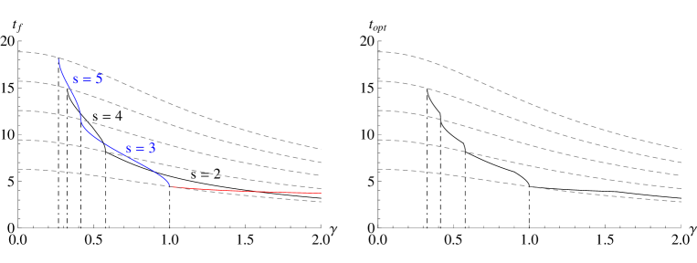
Figure 1: Left plot: comparison of the transition times $t_{f}$ for the extremal trajectories derived in this work, as a function of $\gamma$, when $\omega_{0}=1$. The blue and black lines are associated with the cases of even, respectively odd number of switching times in nonsingular extremal strategies, and the red line corresponds to the singular extremal. The dashed lines represents some upper and lower bounds on $t_{opt}$ as derived in Proposition 2. More precisely, they give $k\frac{\pi}{\omega}$ for $k=2,3,4,5$ and $6$. Right plot: resulting optimal time in the range of values of $\gamma$ where analytical expressions for the extremals are possible.

It is not possible to give the form of the time optimal control and minimum time in a compact way since the optimal solution depends in an intricate way on the relative values of $\omega_{0}$ and $\gamma$. In different situations the optimal solution is given by different types of extremals, singular or nonsingular. This is illustrated in Fig. 1, where the choice $\omega_{0}=1$ has been made, and the extremals which are clearly sub-optimal have been neglected. We summarize our findings in the following theorem, where, on account of Proposition II.1, we provide the result for any operator equivalent to SWAP.

Theorem 3.

Consider the system (I.1). Given a target operator of the form

$$X_{f}=\left(\begin{array}[]{cc}0&e^{i\varphi}\\ -e^{-i\varphi}&0\\ \end{array}\right)$$ (65)

for some $\varphi\in\mathbb{R}$, the optimal control strategy steering $X_{1}$ and $X_{2}$ to $\pm X_{f}$ can be nonsingular or singular, depending on the relative values of $\omega_{0}$ and $\gamma$.

Nonsingular strategies are bang-bang, with $s$ switching times. They are given by

$$u_{x}=\pm\gamma\cos{\varphi},\quad u_{y}=\mp\gamma\sin{\varphi},\quad u_{z}=0,$$ (66)

and both $u_{x}$, $u_{y}$ change sign at $t_{k}=\tilde{t}+k\bar{t}$, with $k=0,1,\ldots,s$. The number $s$ depends on the relative values of $\omega_{0}$ and $\gamma$. The optimal transition time is given by $t_{opt}=2\tilde{t}+(s-1)\bar{t}$ for a given $s$. Analytical expressions of $\tilde{t}$ and $\bar{t}$ are provided in Appendices B and C.

The optimal singular extremal consists of the alternation of a nonsingular arc for time $\tilde{t}$, a singular arc for time $t^{\prime}$, and finally a nonsingular arc for time $\tilde{t}$. The optimal transition time is given by $t_{opt}=2\tilde{t}+t^{\prime}$, and analytical expressions of $\tilde{t}$ and $t^{\prime}$ can be found in Appendix D. The associated control strategy is given by (66) on nonsingular arcs, and $u_{x}\equiv u_{y}\equiv u_{z}\equiv 0$ on the singular arc.

VII Discussion and conclusions

The problem of controlling in minimum time a quantum bit interacting with an additional two level system can be mapped to an equivalent problem of simultaneous control of two quantum bits under the same control field. In this paper, we have solved this problem for the class of SWAP operators, although some of our results apply to the case of an arbitrary final target operations as well. The application of the necessary conditions of optimality, given by the Pontryagin Maximum Principle, leads to the consideration of two type of candidates optimal controls, singular and nonsingular. Our analysis shows that singular extremals can be optimal only in a specific range of control strength, and they must have a particular structure, with a singular arc between two nonsingular arcs. The dynamical analysis benefits from known results from the central force problem. We have found that the optimal control strategy depends in a complicated way on the relative strength of the control and the interaction. These results can be used to synthesize the SWAP operation in minimum time in quantum computation implementations in cases where the target system is interacting with an analogous system, and-or to synthesize the SWAP operation on two systems simultaneously.

Because of the homomorphism between $SU(2)$ and $SO(3)$, we can adapt our results to the derivation of optimal control strategies for rotating a rigid body in $\mathbb{R}^{3}$ in minimum time. The class of SWAP operators in $SU(2)$ corresponds to the class of rotations of angle $\pi$ around axes orthogonal to the axis of the drift dynamics. This is another scenario where our analysis applies.

The specific form of the interaction (Ising) is crucial for the derivation of our results, and for the equivalence of the two problems mentioned above. An interaction term of the form $\sigma_{1}\otimes\sigma_{2}$, with arbitrary $\sigma_{1}$ and $\sigma_{2}$, can be considered under the perspective of driving only one two-level system, the second one representing an undesired disturbance. But in this case this problem is not equivalent to that of simultaneously driving a pair of two-level systems with opposite drifts. Finally, more complicated interaction terms (e.g., the Heisenberg interaction) are not compatible with our procedure.

In our analysis, the drift parameter $\omega_{0}$ and the control strength $\gamma$ can be arbitrarily varied, and we have analytically derived the optimal control strategy and the corresponding time when $\frac{\gamma}{\omega_{0}}$ exceeds a threshold, which is approximatively $0.325$. For smaller control strength, numerical investigations are needed.

We have found that the optimal control strategy for the SWAP operator (or equivalent) always requires $u_{z}=0$, both for nonsingular or singular arcs. Therefore, we can conclude that, for this class of operators, the scenario with only two independent controls $u_{x}$ and $u_{y}$ is completely equivalent to that considered in this work. The same result has been found when investigating the analogous optimal control problem with only one two-level system RR , and it is a consequence of the symmetry of the problem.

Our results add to the growing literature on optimal control of quantum systems. The problem of time optimal simultaneous control of two quantum bits in minimum time does not seem to have been considered earlier. One notable exception is Sugny , where however the problem was set up for the state and not for the evolution operator as here.

Appendix A Numerical analysis supporting Conjecture 1

In this appendix we provide numerical evidence that $L=0$ is a necessary condition for the optimality of extremal trajectories. Without loss of generality, we write the initial condition as $(b_{x}(0),0)$, which, with the choice $E=\frac{\omega^{2}_{0}}{2}$, leads to

$$\dot{b}_{x}(0)=\cos{\vartheta}\sqrt{1-b_{x}(0)^{2}},\qquad\dot{b}_{y}(0)=\sin{\vartheta}\sqrt{1-b_{x}(0)^{2}}$$ (67)

for some $\vartheta$ satisfying $0\leqslant\vartheta\leqslant\pi$. We solve the costate dynamics (III), and from them we derive the corresponding extremal controls (21). Using the extremal controls, we numerically solve Eq.s (I.1) and derive the corresponding extremal trajectories in the Lie group, $X_{1}=X_{1}(t,\vartheta,b_{x}(0))$ and $X_{2}=X_{2}(t,\vartheta,b_{x}(0))$, in the time interval $0\leqslant t\leqslant T$. We then consider the following real functions:

$$F_{+} = F_{+}(t,\vartheta,b_{x}(0))=\frac{1}{4}\Big{[}\Big{(}{\rm Tr}(X_{1}-X_{2})\sigma_{x}\Big{)}^{2}+\Big{(}{\rm Tr}(X_{1}-X_{2})\sigma_{y}\Big{)}^{2}\Big{]},$$

$$F_{-} = F_{-}(t,\vartheta,b_{x}(0))=\frac{1}{4}\Big{[}\Big{(}{\rm Tr}(X_{1}+X_{2})\sigma_{x}\Big{)}^{2}+\Big{(}{\rm Tr}(X_{1}+X_{2})\sigma_{y}\Big{)}^{2}\Big{]},$$ (68)

satisfying $0\leqslant F_{\pm}\leqslant 1$. Moreover, the function $F_{+}$ reaches its maximum if and only if $X_{1}=X_{2}$ matches some operator equivalent to SWAP (according to Proposition II.1), and similarly for $F_{-}$, with $X_{1}=-X_{2}$. Therefore the optimal time $t_{f}$ we want to determine is the smallest time such that $F_{+}=1$ or $F_{-}=1$, and it can be found by gradually increasing the range of numerical integration $[0,T]$. For any choice of $\omega_{0}$ and $\gamma$ that we have considered, we have always found that the smallest time is associated with $\vartheta=0$ or $\pi$, or $b_{x}(0)=0$ or $1$, which means $L=0$. For sake of completeness, some contour plots of $F_{\pm}$ are reported in Fig.s 6 and 7. We do not numerically compute the minimum time $t_{f}$, because once we know that $L=0$ we can obtain an analytical result.

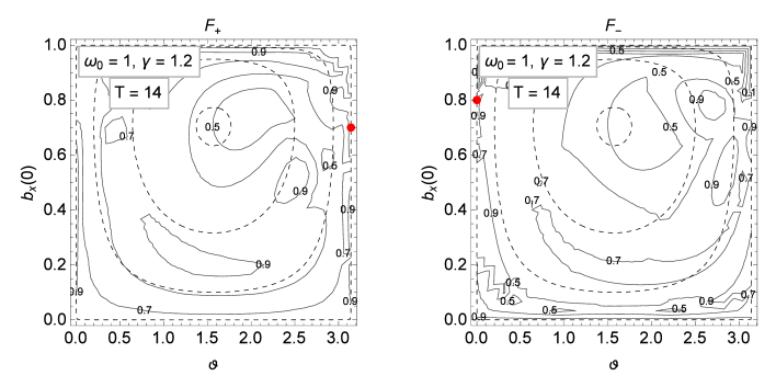
Figure 7: Contour plots of the functions $F_{+}$ and $F_{-}$ for selected values of $\omega_{0}$, $\gamma$ and $T$ (in the inset). The parameters in the two plots are the same, but $T$ which is increased. From the behavior of $F_{-}$, it is apparent the existence of a sub-optimal extremal.

This numerical analysis is fully consistent with the analytical expressions of nonsingular extremals presented in Section IV. With suitable choices of $T$, that is, by sufficiently increasing it, it is possible to investigate the structure of sub-optimal extremal arcs, and, again, we find consistency with our analytical results (see Fig. 7). On one side our numerical computations motivate the analytical evaluation of extremal strategies; on the other, they provide an independent check of these results, since they are fully consistent with them.

Appendix B Analysis of nonsingular extremals for $X_{f}=i\sigma_{y}$

System (52) admits analytical solutions for several values of $n$. We recall that a necessary condition for all these extremals is $X_{2}(t_{f})=-X_{1}(t_{f})$.

The case $n=0$ is the only possible extremal with only one switching time for $u_{x}$. We find that system (52) is inconsistent, with the only exception of the case when $\gamma=\omega_{0}$. In this special case, it must be $\cos{\omega\tilde{\tau}}=0$ and $X_{1}(t_{f})=-X_{f}$, and we find $t_{f}=2\tilde{t}=\sqrt{2}\frac{\pi}{\gamma}$ and $b_{x}(0)$ is unconstrained.

If $n=1$, the extremal control strategies have $3$ switching times. We find that

$$\sin{\omega\bar{\tau}}=\frac{\omega}{2\omega_{0}}\sqrt{\frac{\gamma\pm\omega_{0}}{\gamma}},\quad\sin{\omega\tilde{\tau}}=\frac{\omega}{2\gamma}\sqrt{\frac{\omega_{0}\mp\gamma}{\omega_{0}}},$$ (69)

where the signs of the two terms follows from Proposition IV.1, which implies that $\sin{\omega\bar{\tau}}\geqslant 0$, $\cos{\omega\bar{\tau}}\leqslant 0$, and $\sin{\omega\tilde{\tau}}\geqslant 0$. The upper signs correspond to $X_{1}(t_{f})=X_{f}$, the lower signs to $X_{1}(t_{f})=-X_{f}$. Eq.s (69) are consistent with (IV) and (43) when

$$b_{x}(0)=\sqrt{\left(\frac{\omega_{0}}{\gamma}\right)^{2}-\frac{\gamma\pm\omega_{0}}{3\gamma\mp\omega_{0}}}.$$ (70)

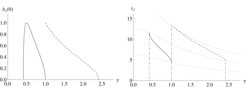
Figure 2: Plots of $b_{x}(0)$ and $t_{f}$ as functions of the control strength $\gamma$, with $\omega_{0}=1$, $X_{f}=i\sigma_{y}$ and $n=1$. Dashed lines are associated with extremals which are certainly sub-optimal.

These solutions exist only when $\sqrt{2}-1\leqslant\frac{\gamma}{\omega_{0}}\leqslant 1$, if we consider the upper sign, and when $1\leqslant\frac{\gamma}{\omega_{0}}\leqslant\sqrt{2}+1$ if we consider the lower sign (otherwise the two functions in (69) are not defined, or $b_{x}(0)<0$). The total time for the transition is given by $t_{f}=2(\tilde{t}+\bar{t})$. For $X_{1}(t_{f})=X_{f}$ we find

$$t_{f}=\frac{4}{\sqrt{\omega_{0}^{2}+\gamma^{2}}}\left(\pi-\arcsin{\frac{\omega}{2\omega_{0}}\sqrt{\frac{\gamma+\omega_{0}}{\gamma}}}+\arcsin{\frac{\omega}{2\gamma}\sqrt{\frac{\omega_{0}-\gamma}{\omega_{0}}}}\right).$$ (71)

Similarly, for the transition $X_{1}(t_{f})=-X_{f}$ we obtain

$$t_{f}=\frac{4}{\sqrt{\omega_{0}^{2}+\gamma^{2}}}\left(2\pi-\arcsin{\frac{\omega}{2\omega_{0}}\sqrt{\frac{\gamma-\omega_{0}}{\gamma}}}-\arcsin{\frac{\omega}{2\gamma}\sqrt{\frac{\omega_{0}+\gamma}{\omega_{0}}}}\right).$$ (72)

In (71) and (72), we have used the fact that the sign of $\cos{\omega\tilde{\tau}}$ is determined by the third equation of (52): it is positive in the first case, negative in the second case. Plots of $b_{x}(0)$ and $t_{f}$ as functions of $\gamma$ are shown in Fig. 2.

If $n=2$, the extremal control strategies have $5$ switching times. By expressing $\cos{4\alpha}$ and $\sin{4\alpha}$ in terms of $\sin{\alpha}$ and $\cos{\alpha}$, we rewrite system (52) as

$$\left\{\begin{array}[]{l}1-8\sin^{2}{\alpha}\left(1-\sin^{2}{\alpha}\right)=\mp 2\frac{\omega_{0}\gamma}{\omega^{2}}\sin^{2}{\omega\tilde{\tau}}\\ 4\frac{\gamma}{\omega_{0}}\sin^{2}{\alpha}\left(1-2\sin^{2}{\alpha}\right)=\pm\left(1-2\left(\frac{\gamma}{\omega}\right)^{2}\sin^{2}{\omega\tilde{\tau}}\right)\\ 4\sin{\alpha}\left(1-2\sin^{2}{\alpha}\right)\cos{\omega\bar{\tau}}=\mp\frac{\gamma}{\omega}\sin{2\omega\tilde{\tau}}\end{array}\right..$$ (73)

From the first and second equation we derive the biquadratic equation in $\sin{\alpha}$,

$$\sin^{4}{\alpha}-\frac{3}{4}\sin^{2}{\alpha}+\frac{\omega_{0}\pm\gamma}{16\gamma}=0,$$ (74)

which admits four solutions. If $X_{1}(t_{f})=X_{f}$, we obtain

$$\sin{\alpha}=\frac{1}{2}\sqrt{\frac{3}{2}\pm\sqrt{\frac{5}{4}-\frac{\omega_{0}}{\gamma}}}.$$ (75)

Conversely, if $X_{1}(t_{f})=-X_{f}$, we find

$$\sin{\alpha}=\frac{1}{2}\sqrt{\frac{3}{2}\pm\sqrt{\frac{5}{4}+\frac{\omega_{0}}{\gamma}}}.$$ (76)

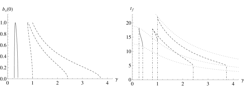
Figure 3: Plots of $b_{x}(0)$ and $t_{f}$ as functions of the control strength $\gamma$, with $\omega_{0}=1$, $X_{f}=i\sigma_{y}$ and $n=2$. Dashed lines are associated with extremals which are certainly sub-optimal.

From Eq. (IV.1) we can find $\sin{\omega\bar{\tau}}$, and moreover, from the first equation in (73), by choosing the suitable signs, and rewriting the left hand side as $\cos{4\alpha}$ for simplicity, we can evaluate

$$\sin{\omega\tilde{\tau}}=\sqrt{\mp\frac{\omega^{2}}{2\omega_{0}\gamma}\cos{4\alpha}}.$$ (77)

These conditions are consistent with (IV) and (43) as long as

$$b_{x}(0)=\sqrt{\frac{\omega_{0}^{2}-\omega^{2}\sin^{2}{\alpha}}{\gamma^{2}\cos^{2}{\alpha}}}.$$ (78)

Now, by requiring $0\leqslant\sin{\alpha}\leqslant 1$ and $0\leqslant b_{x}(0)\leqslant 1$, it is possible to prove that all the solutions of (74) are consistent, and to determine the associated ranges of $\frac{\gamma}{\omega_{0}}$, which are not reported here because they are not needed for further developments. The final times associated to these four extremals are given by $t_{f}=2\tilde{t}+4\bar{t}$, that is

$$t_{f}=\frac{2}{\sqrt{\omega_{0}^{2}+\gamma^{2}}}\left(4\pi+2\arcsin{\sqrt{\mp\frac{\omega^{2}}{2\omega_{0}\gamma}\cos{4\alpha}}}-4\arcsin{\left(\frac{\omega}{\omega_{0}}\sin{\alpha}\right)}\right).$$ (79)

Plots of $b_{x}(0)$ and $t_{f}$ for these four extremal trajectories are shown in Fig. 3. Our development shows that the only extremal which can contribute to optimal solutions corresponds to the solution with positive sign in Eq. (76), which is associated with $X_{1}(t_{f})=-X_{f}$.

Appendix C Analysis of nonsingular extremals for $X_{f}=i\sigma_{x}$

We compute the analytical solution of system (57) in the simplest cases. We recall that in this case it must be $X_{1}(t_{f})=X_{2}(t_{f})=X_{f}$.

If $n=0$, the extremal control strategies have $2$ switching times. By considering the definitions (IV.1), the system is rewritten as

$$\left\{\begin{array}[]{l}\cos{\omega\bar{\tau}}=\mp\frac{\gamma}{\omega}\sin{2\omega\tilde{\tau}}\\ \frac{\gamma}{\omega}\sin{\omega\bar{\tau}}=\pm\left(1-2\left(\frac{\gamma}{\omega}\right)^{2}\sin^{2}{\omega\tilde{\tau}}\right)\\ \frac{\omega_{0}}{\omega}\sin{\omega\bar{\tau}}=\pm 2\frac{\omega_{0}\gamma}{\omega^{2}}\sin^{2}{\omega\tilde{\tau}}\end{array}\right..$$ (80)

Consider the case of upper signs in (80), that is, final operator $X_{1}(t_{f})=X_{f}$. Since $\omega_{0}\neq 0$, we find $\sin{\omega\tilde{\tau}}=\pm\frac{\omega}{2\gamma}$ and $\sin{\omega\bar{\tau}}=\frac{\omega}{2\gamma}$, which are well defined only when $\frac{\omega}{2\gamma}\leqslant 1$, or $\frac{\gamma}{\omega_{0}}\geqslant\frac{1}{\sqrt{3}}$. Moreover, from $\sin{\omega\tilde{\tau}}=\pm\sin{\omega\bar{\tau}}$ and the first equation in (80), we find that $\cos{\omega\tilde{\tau}}=\mp\cos{\omega\bar{\tau}}$. We conclude that $\cos{\omega\tilde{t}}=\cos{\omega\bar{t}}$ and $\sin{\omega\tilde{t}}=-\sin{\omega\bar{t}}$. These are constraints on the switching times, which must be consistent with the expressions (IV) and (43). By using the explicit expressions on $A_{0}$, $B_{0}$ and $C_{0}$, we find that the initial condition of the costate must satisfy

$$b_{x}(0)=\frac{\omega_{0}}{\gamma}\sqrt{\frac{(\omega_{0}^{2}-2\gamma^{2})^{2}-\gamma^{4}}{(\omega_{0}^{2}-2\gamma^{2})^{2}-\omega_{0}^{2}\gamma^{2}}}.$$ (81)

Therefore, this extremal is well defined when $\gamma\geqslant\frac{1}{\sqrt{3}}\omega_{0}$, and the total time for the transition is given by $t_{f}=2\tilde{t}+\bar{t}$, or more explicitly

$$t_{f}=\frac{2}{\sqrt{\omega_{0}^{2}+\gamma^{2}}}\left(\pi+\arctan{\sqrt{\frac{\omega_{0}^{2}+\gamma^{2}}{3\gamma^{2}-\omega_{0}^{2}}}}\right).$$ (82)

The case with final operator $X_{1}(t_{f})=-X_{f}$ is obtained by replacing $\tau$ with $\tau+\pi$ in the previous formulas. However, the result $\sin{\omega\bar{\tau}}=-\frac{\omega}{2\gamma}<0$ is inconsistent with the conditions expressed in Proposition IV.1, therefore there are no extremal trajectories in this case. See Fig. 4 for plots of $b_{x}(0)$ and $t_{f}$ in this case.

If $n=1$, the extremal control strategies have $4$ switching times, and the system (57) becomes

$$\left\{\begin{array}[]{l}\left(4\sin^{2}{\alpha}-1\right)\cos{\omega\bar{\tau}}=\pm\frac{\gamma}{\omega}\sin{2\omega\tilde{\tau}}\\ \frac{\gamma}{\omega_{0}}\left(1-4\sin^{2}{\alpha}\right)\sin{\alpha}=\pm\left(1-2\left(\frac{\gamma}{\omega}\right)^{2}\sin^{2}{\omega\tilde{\tau}}\right)\\ \sin{\alpha}\left(3-4\sin^{2}{\alpha}\right)=\pm 2\frac{\omega_{0}\gamma}{\omega^{2}}\sin^{2}{\omega\tilde{\tau}}\end{array}\right..$$ (83)

From the second and third equation of this system we get a depressed cubic equation in $\sin{\alpha}$,

$$\sin^{3}{\alpha}+p\sin{\alpha}+q=0,$$ (84)

where

$$p=-\frac{1}{2},\qquad q=\pm\frac{\omega_{0}}{8\gamma}.$$ (85)

This equation can be solved by using the Cardano’s method. By defining $u$ and $v$ such that $u+v=\sin{\alpha}$, we find $u^{3}+v^{3}=-q$ and $3uv=-p$, we find that both $u^{3}$ and $v^{3}$ satisfy the equation

$$z^{2}+qz-\Big{(}\frac{p}{3}\Big{)}^{3}=0.$$ (86)

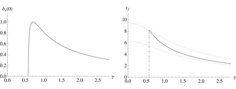
Figure 4: Plots of $b_{x}(0)$ and $t_{f}$ as functions of the control strength $\gamma$, with $\omega_{0}=1$, $X_{f}=i\sigma_{x}$ and $n=0$. Dashed lines are associated with extremals which are certainly sub-optimal.

Then we solve this quadratic equation and get $u^{3}$ and $v^{3}$, extract the cubic roots, and impose the further requirement $3uv=-p$. We are interested in real roots of the original cubic equation, and their number depend on the sign of the discriminant $\Delta=-27q^{2}-4p^{3}$. If $\Delta<0$, there is only one real root; if $\Delta=0$ there are three real roots with degeneration, and finally if $\Delta>0$ there are three distinct real roots. By considering the values of $p$ and $q$ in (85), we conclude that, if $\frac{\gamma}{\omega_{0}}<\frac{3}{4}\sqrt{\frac{3}{2}}$, the only real root is given by

$$\sin{\alpha}=\sqrt[3]{-\frac{q}{2}+\sqrt{\Big{(}\frac{q}{2}\Big{)}^{2}+\Big{(}\frac{p}{3}\Big{)}^{3}}}+\sqrt[3]{-\frac{q}{2}-\sqrt{\Big{(}\frac{q}{2}\Big{)}^{2}+\Big{(}\frac{p}{3}\Big{)}^{3}}},$$ (87)

where we consider the real cubic root. Since it must be $\sin{\alpha}\geqslant 0$, we require $q\leqslant 0$, and then the only possibility is $X_{1}(t_{f})=-X_{f}$, corresponding to the lower sign in (83) and (85). If $\frac{\gamma}{\omega_{0}}\geqslant\frac{3}{4}\sqrt{\frac{3}{2}}$, all the roots are real, and their general expressions are

$$(\sin{\alpha})_{k}=2\sqrt{-\frac{p}{3}}\cos{\Big{(}\delta+\frac{2k}{3}\pi}\Big{)},$$ (88)

with $k=0,1,2$, and

$$\delta=-\frac{1}{3}\arctan{\frac{1}{3q}\sqrt{\frac{\Delta}{3}}}.$$ (89)

In the given range of parameters, $\sin{3\alpha}$ is positive for $k=0$ and negative for $k=1,2$. Therefore, in the first case we have to consider the upper signs in (83) and (85), leading to $X_{1}(t_{f})=X_{f}$, and the lower signs otherwise, with $X_{1}(t_{f})=-X_{f}$.

The requirements $0\leqslant\sin{\alpha}\leqslant 1$ and $0\leqslant\sin{\omega\bar{\tau}}\leqslant 1$ further restrict the range of admissible values for $\frac{\gamma}{\omega_{0}}$. Their explicit expression are cumbersome and unnecessary; we only mention that extremal trajectories associated to the case $k=0$ in (88) are impossible because of the constraint $\sin{\omega\bar{\tau}}\leqslant 1$. Therefore, $X_{1}(t_{f})=-X_{f}$ is the only possible final operation. By solving the last equation in (83) we find

$$\sin{\omega\tilde{\tau}}=\sqrt{-\frac{\omega^{2}}{2\omega_{0}\gamma}\sin{3\alpha}},$$ (90)

which is well defined because $\sin{3\alpha}\leqslant 0$. The conditions (87) and (90) are consistent with (IV) and (43) as long as (78) is satisfied. The total time for the transition on this extremal trajectory is given by $t_{f}=2\tilde{t}+3\bar{t}$, that is

$$t_{f}=\frac{2}{\sqrt{\omega_{0}^{2}+\gamma^{2}}}\left(3\pi+2\arcsin{\sqrt{-\frac{\omega^{2}}{2\omega_{0}\gamma}\sin{3\alpha}}}-3\arcsin{\left(\frac{\omega}{\omega_{0}}\sin{\alpha}\right)}\right).$$ (91)

Fig. 5 shows plots of $b_{x}(0)$ and $t_{f}$ for this class of extremals. According to the analysis of Section VI, the only extremal which can be optimal is the one characterized by (87).

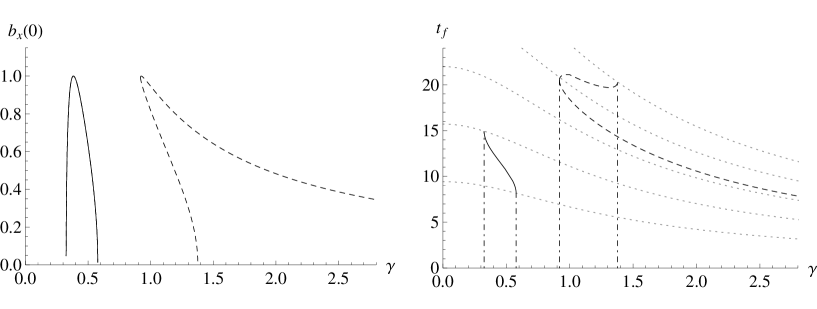
Figure 5: Plots of $b_{x}(0)$ and $t_{f}$ as functions of the control strength $\gamma$, with $\omega_{0}=1$, $X_{f}=i\sigma_{x}$ and $n=1$. Dashed lines are associated with extremals which are certainly sub-optimal.

Appendix D Analysis of singular extremals

Considering the two terms in (61), and assuming that $B_{0}\leqslant 0$, we can be recast the final result in a rather compact form as

$$X_{1}(t) = -\Big{(}\sin{\eta}\sin{(\xi_{+}+\eta)}-\cos{\varphi}\cos{(\xi_{+}+\varphi)}\Big{)}I+$$ (92)

$$- \frac{i}{2}\Big{(}(1-\cos{2\varphi})\cos{(\xi_{+}+\eta)}+\sin{2\varphi}\sin{(\xi_{+}+\eta)}\Big{)}\sigma_{x}+$$

$$- \frac{i}{2}\Big{(}(1+\cos{2\varphi})\sin{(\xi_{+}+\eta)}+\sin{2\varphi}\cos{(\xi_{+}+\eta)}\Big{)}\sigma_{y}+$$

$$- i\Big{(}\sin{\eta}\cos{(\xi_{+}+\eta)}-\sin{\varphi}\cos{(\xi_{+}+\varphi)}\Big{)}\sigma_{z}$$

and

$$X_{2}(t) = +\Big{(}\sin{\eta}\sin{(\xi_{-}-\eta)}+\cos{\varphi}\cos{(\xi_{-}+\varphi)}\Big{)}I+$$ (93)

$$- \frac{i}{2}\Big{(}(1-\cos{2\varphi})\cos{(\xi_{-}-\eta)}+\sin{2\varphi}\sin{(\xi_{-}-\eta)}\Big{)}\sigma_{x}+$$

$$- \frac{i}{2}\Big{(}(1+\cos{2\varphi})\sin{(\xi_{-}-\eta)}+\sin{2\varphi}\cos{(\xi_{-}-\eta)}\Big{)}\sigma_{y}+$$

$$+ i\Big{(}\sin{\eta}\cos{(\xi_{-}-\eta)}+\sin{\varphi}\cos{(\xi_{-}+\varphi)}\Big{)}\sigma_{z}$$

where we have defined the two functions

$$\xi_{\pm}=\xi_{\pm}(t^{\prime})=\frac{1}{2}\left(\int_{0}^{t^{\prime}}u_{z}(s)ds\pm\omega_{0}t^{\prime}\right)$$ (94)

and $\eta\in(0,\frac{\pi}{2})$ satisfies

$$\sin{\eta}=\frac{\omega_{0}}{\gamma},\qquad\cos{\eta}=\frac{1}{\gamma}\sqrt{\gamma^{2}-\omega_{0}^{2}}.$$ (95)

Since $u_{z}$ enters the problem only through the integral in (94), without loss of generality we can assume it is constant on the singular arc. Therefore $\xi_{\pm}=\frac{1}{2}(u_{z}\pm\omega_{0})t^{\prime}$. The free parameters in (92) and (93) are $\varphi$ and $\xi_{\pm}$ (or, which is the same, $\varphi$, $u_{z}$ and $t^{\prime}$). Target operators equivalent to SWAP have the form

$$X_{f}=ie^{i\varphi S_{z}}\sigma_{y}e^{-i\varphi S_{z}}=i(\sin{\varphi}\sigma_{x}+\cos{\varphi}\sigma_{y}),$$ (96)

and, by requiring $X_{1}=\pm X_{f}$ we find the system

$$\left\{\begin{array}[]{l}\sin{\eta}\sin{(\xi_{+}+\eta)}-\cos{\varphi}\cos{(\xi_{+}+\varphi)}=0\\ (1-\cos{2\varphi})\cos{(\xi_{+}+\eta)}+\sin{2\varphi}\sin{(\xi_{+}+\eta)}=\mp 2\sin{\varphi}\\ (1+\cos{2\varphi})\sin{(\xi_{+}+\eta)}+\sin{2\varphi}\cos{(\xi_{+}+\eta)}=\mp 2\cos{\varphi}\\ \sin{\eta}\cos{(\xi_{+}+\eta)}-\sin{\varphi}\cos{(\xi_{+}+\varphi)}=0\end{array}\right.$$ (97)

From the first and fourth equations we find that $\cos{(\xi_{+}+\varphi)}=\pm\sin{\eta}$, and consequently $\sin(\xi_{+}+\eta)=\pm\cos{\varphi}$ and $\cos(\xi_{+}+\eta)=\pm\sin{\varphi}$. We observe that the second and third equations in (97) reduce to identities. Finally, the solution of (97) is expressed as

$$\cos{\xi_{+}}=\pm\sin{(\varphi+\eta)},\qquad\sin{\xi_{+}}=\pm\cos{(\varphi+\eta)}.$$ (98)

For solving $X_{2}=\pm X_{f}$, we follow the same steps. We find that

$$\cos{\xi_{-}}=\mp\sin{(\varphi-\eta)},\qquad\sin{\xi_{-}}=\mp\cos{(\varphi-\eta)}.$$ (99)

Since the signs in (98) and (99) are opposite, the only consistent solutions must satisfy $X_{1}=-X_{2}=X_{f}$, with $X_{f}$ as in (96) for some $\varphi$. By combining Eq.s (98) and (99), we find that $u_{z}t^{\prime}=2\pi-2\varphi+4k\pi$ or $u_{z}t^{\prime}=4\pi-2\varphi+4k\pi$ for some integer $k$, and $\omega_{0}t^{\prime}=\pi-2\eta+4l\pi$ or $\omega_{0}t^{\prime}=3\pi-2\eta+4l\pi$ for some integer $l\geqslant 0$. We are interested in the solution with minimum time $t^{\prime}$, with the additional constraint that $|u_{z}|\leqslant\gamma$. This minimum is obtained when $\varphi=0$, $k=-1$ and $l=0$, that is, $\omega_{0}t^{\prime}=\pi-2\eta$ and $u_{z}=0$. This means that, on singular arcs on extremal trajectories, the evolution is given by the drift term.

Summing up, the total time for the transition $X\rightarrow X_{f}=i\sigma_{y}$ is given by $t_{f}=2\tilde{t}+t^{\prime}$, where $\tilde{t}$ is determined by (60). The explicit expression in terms of $\omega_{0}$ and $\gamma$ is

$$t_{f}=\frac{2}{\sqrt{\omega_{0}^{2}+\gamma^{2}}}\left(\pi-\arccos{\left(\frac{\omega_{0}}{\gamma}\right)^{2}}\right)+\frac{1}{\omega_{0}}\left(\pi-2\arcsin{\frac{\omega_{0}}{\gamma}}\right).$$ (100)

When $B_{0}>0$, the analysis is completely analogous. The dynamics in the Lie group is described by the following equations:

$$X_{1}(t) = +\Big{(}\sin{\eta}\sin{(\xi_{+}-\eta)}+\cos{\varphi}\cos{(\xi_{+}+\varphi)}\Big{)}I+$$ (101)

$$+ \frac{i}{2}\Big{(}(1-\cos{2\varphi})\cos{(\xi_{+}-\eta)}+\sin{2\varphi}\sin{(\xi_{+}-\eta)}\Big{)}\sigma_{x}+$$

$$+ \frac{i}{2}\Big{(}(1+\cos{2\varphi})\sin{(\xi_{+}-\eta)}+\sin{2\varphi}\cos{(\xi_{+}-\eta)}\Big{)}\sigma_{y}+$$

$$+ i\Big{(}\sin{\eta}\cos{(\xi_{+}-\eta)}+\sin{\varphi}\cos{(\xi_{+}+\varphi)}\Big{)}\sigma_{z}$$

and

$$X_{2}(t) = -\Big{(}\sin{\eta}\sin{(\xi_{-}+\eta)}-\cos{\varphi}\cos{(\xi_{-}+\varphi)}\Big{)}I+$$ (102)

$$+ \frac{i}{2}\Big{(}(1-\cos{2\varphi})\cos{(\xi_{-}+\eta)}+\sin{2\varphi}\sin{(\xi_{-}+\eta)}\Big{)}\sigma_{x}+$$

$$+ \frac{i}{2}\Big{(}(1+\cos{2\varphi})\sin{(\xi_{-}+\eta)}+\sin{2\varphi}\cos{(\xi_{-}+\eta)}\Big{)}\sigma_{y}+$$

$$- i\Big{(}\sin{\eta}\cos{(\xi_{-}+\eta)}-\sin{\varphi}\cos{(\xi_{-}+\varphi)}\Big{)}\sigma_{z}.$$

As before, the only consistent requirement is $X_{1}=-X_{2}=X_{f}$, and the solution is given by

$$\cos{\xi_{-}}=\pm\sin{(\varphi+\eta)},\qquad\sin{\xi_{-}}=\pm\cos{(\varphi+\eta)}.$$ (103)

For solving $X_{2}=\pm X_{f}$, we follow the same steps. We find that

$$\cos{\xi_{+}}=\mp\sin{(\varphi-\eta)},\qquad\sin{\xi_{+}}=\mp\cos{(\varphi-\eta)}.$$ (104)

By combining these equations, we find that $u_{z}t^{\prime}=2\pi-2\varphi+4k\pi$ or $u_{z}t^{\prime}=4\pi-2\varphi+4k\pi$ for some integer $k$, and $\omega_{0}t^{\prime}=\pi+2\eta+4l\pi$ or $\omega_{0}t^{\prime}=3\pi+2\eta+4l\pi$ for some integer $l\geqslant 0$. These extremals are certainly not optimal, as both $\tilde{t}$ and $t^{\prime}$ are larger than the corresponding quantities derived in the case $B_{0}\leqslant 0$.

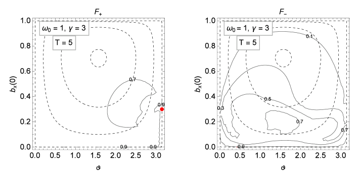
Figure 6: Contour plots of the functions $F_{+}$ and $F_{-}$ for selected values of $\omega_{0}$, $\gamma$ and $T$ (in the inset). The dashed lines represent points with a fixed value for $L$, decreasing towards the border of the plot, where $L=0$. The red spots shows the values of $b_{x}(0)$ and $\vartheta$ such that $F_{\pm}=1$ with $0\leqslant t\leqslant T$.

References

- (1) F. Albertini and D. D’Dalessandro, J. Math. Phys. 56, 012106 (2015)
- (2) R. Romano, Phys. Rev. A 90, 062302 (2014)
- (3) M. A. Nielsen and I. L. Chuang, Quantum Computation and Quantum Information, Cambridge University Press, Cambridge, U.K., New York (2000)
- (4) M. H. Levitt, Spin dynamics: basics of nuclear magnetic resonance, John Wiley and sons, New York-London-Sydney (2008)
- (5) R. Wu, C. Li and Y. Wang, Phys. Lett. A 295, 20 (2002)
- (6) U. Boscain and P. Mason, J. Math. Phys. 47, 062101 (2006)
- (7) M. Wenin and W. Pötz, Phys. Rev. A 74, 022319 (2006)
- (8) A. Carlini, A. Hosoya, T. Koike and Y. Okudaira, Phys. Rev. A 75, 042308 (2007)
- (9) E. Kirillova, T. Hoch and K. Spindler, WSEAS Trans. Math. 7, 687 (2008)
- (10) A. Garon, S. J. Glaser and D. Sugny, Phys. Rev. A 88 043422 (2013)
- (11) G. C. Hegerfeldt, Phys. Rev. Lett. 111, 260501 (2013)
- (12) C.D. Aiello, M. Allegra, B. Hemmerling, X. Wang and Paola Cappellaro, ArXiv:1410.4975 (2014)
- (13) B. Russell and S. Stepney, J. of Phys. A 48, 115303 (2015)
- (14) D.A. Lidar, Adv. Chem. Phys. 154, 295 (2014)
- (15) G. de Lange, T. van der Sar, M.S. Blok, Z.H. Wang, V.V. Dobrovitski and R. Hanson, Scientific Reports 2, 382 (2012)
- (16) T. H. Taminiau, J.J.T. Wagenaar, T. van der Sar, F. Jelezko, V.V. Dobrovitski and R. Hanson, Phys. Rev. Lett. 109, 137602 (2012)
- (17) C. Arenz, G. Gualdi and D. Burgarth, New J. Phys. 16, 065023 (2014)
- (18) L. Pontryagin et V. G. Boltyanskii, Mathematical theory of optimal processes, Mir, Moscou (1974)
- (19) W. Fleming and R. Rishel, Deterministic and Stochastic Optimal Control, Applications of Mathematics, Springer-Verlag, New York, 1975
- (20) U. Boscain and B. Piccoli, Optimal Syntheses for Control Systems on 2-D Manifolds, Springer SMAI 43 (2004)
- (21) R. Wu, R. Long, J. Dominy, T.S. Ho and H. Rabitz, Phys. Rev. A 86, 013405 (2012)
- (22) M. Lapert, Y. Zhang, M. Braun, S. J. Glaser and D. Sugny, Phys. Rev. Lett. 104, 083001 (2010)
- (23) R. Broucke, Astrophisics and Space Science 72, 33 (1980)
- (24) D. D’Alessandro, Introduction to Quantum Control and Dynamics, CRC Press, Boca Raton FL (2007)
- (25) N. Khaneja, R. Brockett and S.J. Glaser, Phys. Rev. A 63, 032308 (2001)
- (26) D. D Alessandro and M. Dahleh, IEEE Trans. A. C. 46, 866 (2001)
- (27) R. Huneault, Time Optimal Control of Closed Quantum Systems, Master thesis, Department of Mathematics, University of Waterloo, Ontario, Canada, 2009
- (28) E. Assemat, M. Lapert, Y. Zhang, M. Braun, S.J. Glaser and D. Sugny, Phys. Rev. A 82, 013415 (2010)