KEK-TH-1811

Accidental Kähler Moduli Inflation

Anshuman Maharana¹, Markus Rummel² and Yoske Sumitomo³,

¹Harish Chandra Research Institute,Chhatnag Road, Jhunsi, Allahabad, UP 211019, India

²Rudolph Peierls Centre for Theoretical Physics, University of Oxford,

1 Keble Road, Oxford, OX1 3NP, United Kingdom

³ High Energy Accelerator Research Organization, KEK,

1-1 Oho, Tsukuba, Ibaraki 305-0801 Japan

Email: anshumanmaharana at hri.res, markus.rummel at physics.ox.ac.uk,
sumitomo at post.kek.jp

1 Introduction

Recent observations in cosmology strongly support the mechanism of inflation [1, 2, 3]. During the inflationary epoch, there is an approximately exponential growth of the scale factor, and the quantum fluctuations of the early universe seed the temperature fluctuations in the cosmic microwave background we observe today. The Planck collaboration measured the value of the spectral index of primordial curvature perturbations precisely, suggesting the behavior of weakly broken scale invariance which is typical in models of inflation [2, 3]. The next experimental goal is to measure the tensor amplitude which is related to the scale of inflation and the displacement of the inflaton in field space. There have been many attempts to measure the tensor-to-scalar ratio, and the upper bound from the combined data is currently given by $r_{0.002}<0.11$ [2, 3, 4]. There is much hope that this upper bound will be improved and we will detect a signal for tensor modes soon as significant efforts in the observational front in the near future are being spent towards the detection of primordial B-mode signals (see e.g. [5] and [6]).

Inflation is a high-energy phenomena. The energy density during inflation is related to the tensor to scalar ratio by $V^{1/4}\sim{\cal O}(0.01)r^{1/4}M_{P}$ when the COBE normalization is applied. Even for small values of $r$, the energy scale is not very far away from Planck scale. Furthermore, the slow-roll conditions make inflation ultra-violet sensitive. This makes it essential to embed inflationary models in an ultra violet complete theory. String theory is the leading candidate for providing us with a theory of quantum gravity. It provides the arena necessary for consistent inflationary model building. There have been a large amount of works on inflation in string theory (see reviews [7, 8, 9]). A particularly attractive setting are IIB flux compactifications [10, 11], where moduli stabilization is well developed.

In this paper, we develop a model of inflection point inflation proposed in [12, 13] with a Kähler modulus in a IIB flux compactification playing the role of the inflaton. Inflation should begin in a small region around the flat enough inflection point by some accident, and hence is sometimes called accidental inflation [14]. Accidental inflation has been studied in several contexts in string theory. Since string compactifications give rise to complicated potentials, one can expect that an appropriate inflection point which leads to prolonged inflation (avoiding the $\eta$ problem of [15]) exists in the vast moduli space. Familiar examples include D-brane inflation which regards the inflaton field as the location of a mobile D-brane in a warped throat [16, 17, 18, 19, 20, 15]. In the warped D-brane inflation, the compactification and moduli stabilization generate significant contributions to the inflaton potential [21, 22, 23], and hence we may have an appropriate inflection point where the slow-roll conditions are met [24, 25, 26, 27, 28] (see also [29]). There are, on the other hand, some attempts realizing accidental inflation by an F-term potential in type IIB, in which inflation ends at the KKLT-based de-Sitter minimum ($dS$) [14] and at the Kähler Uplift $dS$ [30] (see also [31]). String-loop corrections have been used to realize an inflection point potential along the overall volume direction [32]. In this paper, we will use two types of racetrack models to realize accidental inflation: the ordinary racetrack with multiple non-perturbative effects for a single modulus in the superpotential and the recently proposed D-term generated racetrack model [33], both of which are based on the Large Volume Scenario (LVS) for moduli stabilization [34].

The simplest model of inflation in the LVS involving a Kähler modulus is Kähler Moduli Inflation [35]. In this model, the inflation direction is the real part of a Kähler modulus which rolls down towards the LVS minimum. One of the advantages of this model is that we know how inflation ends so that the resultant reheating mechanism may be understood easily once the matter sector is given. However, in this model there is the concern that string-loop corrections to supergravity may spoil the inflationary dynamics (see e.g. [36, 37]). The leading order string-loop correction can be analyzed explicitly when D7-branes wrap the inflationary cycle. Similar effects can also be potentially generated by euclidean D3-branes [9]. The basic reason for the problem is the following. Inflation occurs at a large value of the Kähler modulus to realize a sufficiently flat potential. Since the term depending on the inflaton field is exponentially suppressed, string-loop corrections that are suppressed by a power law function of the inflaton, can dominate over the inflationary potential and spoil its flatness. To get a successful model, one has to embed the model in a compactification in which the loop corrections are tuned small by a small string coupling value or absent by a special brane setup [36, 37].

Although the string-loop corrections may also be present, the concern of spoiling the flatness of the inflationary potential is alleviated in our accidental inflation model. The accidental point is located near the minimum, suitable for prolonged inflation, given an appropriate set of coefficients in the racetrack model. Around the accidental point, the racetrack terms are tuned such that the slow-roll conditions are satisfied by a cancellation between these terms. Owing to this cancellation, the resultant exponential suppression and hence overall size of each racetrack term becomes modest. Once there appears a contribution of string-loop corrections, it can be made easily the same order or less than each of the racetrack term with a reasonable value of the string coupling. The corrections can easily be absorbed by a slight shift of some coefficients of the racetrack potential, while this is difficult in the original Kähler Moduli Inflation model unless having a significant suppression via the string coupling or a special brane setup prohibiting the corrections themselves. The coefficients of the racetrack terms depend on the complex structure moduli, which in turn are determined by flux quanta. Therefore the slight shift of coefficients, corresponding to slightly different flux quanta, would be conceivable in a landscape of flux compactifications.

Furthermore, the hierarchy of gauge group ranks $N$ in non-perturbative terms ($a_{\rm inf}/a_{\rm stab}=N_{\rm stab}/N_{\rm inf}$), that is required between the stabilization and inflation potentials in Kähler Moduli Inflation ($a_{\rm inf}/a_{\rm stab}\sim{\cal O}(10)$) [35], is relaxed in the racetrack models to be $a_{\rm inf}/a_{\rm stab}\sim{\cal O}(1)$. Notably, the effect of this relaxation of hierarchy is more significant in the case of the D-term generated racetrack model. It is clear that the ratio of the gauge group ranks $a_{\rm inf}/a_{\rm stab}\sim{\cal O}(1)$ is more easily realized generically in string compactifications and introduces less fields in the effective field theory as smaller gauge group ranks $N$ are sufficient.

This paper is organized as follows. In Section 2, we illustrate the features of the Accidental Kähler Moduli Inflation in the D-term generated racetrack model, starting with the review of original Kähler Moduli Inflation. In Section 3, the superpotential racetrack model is analyzed and compared with the results of the D-term generated racetrack model. We relegate some of the technical details to Appendix A.

2 Accidental Kähler Moduli Inflation

In this section, we will present our model of accidental inflation with a Kähler modulus as the inflaton. The potential will have a racetrack structure generated by a D-term constraint, which was proposed in [33], and will give rise to an accidental inflection point appearing near the uplifted LVS minimum. This scenario relaxes the concern of Kähler Moduli Inflation that the string-loop corrections to the potential spoil the flatness of the F-term inflation potential. We first start with a review of the D-term generated racetrack model and Kähler Moduli Inflation.

2.1 D-term generated racetrack

We start from a model in type IIB string theory with several Kähler moduli, defined by

$$\begin{split}&K=-2\ln\left(\mathcal{V}+{\xi\over 2}\right),\quad\mathcal{V}=(T_{1}+\bar{T}_{1})^{3/2}-\sum_{i=2}^{5}(T_{i}+\bar{T}_{i})^{3/2},\\ &W=W_{0}+\sum_{i=2}^{5}A_{i}e^{-a_{i}T_{i}},\end{split}$$ (2.1)

and the F-term scalar potential $V_{F}=e^{K}(|D_{I}W|^{2}-3|W|^{2})$. For simplicity, we have omitted the coefficients in the volume, given by the triple intersections of the Calabi-Yau manifold $X_{3}$, which do not affect our result crucially. The parameter $\xi\propto-\chi g_{s}^{-3/2}$ is the leading $\alpha^{\prime}$-correction [38] with the Euler number $\chi$ of $X_{3}$. As we are interested in the parameter region of the LVS [34], any non-perturbative term generated on $T_{1}$ is negligibly small. The Kähler moduli fields are complex holomorphic fields, which we write as $T_{I}=\tau_{I}+i\theta_{I}$ conventionally.

Recently, in the context of uplifting LVS vacua to de Sitter, a new type of racetrack structure was proposed by using a D-term constraint [33]. When we have magnetized D7-branes wrapping the divisor $D_{D}$ in the Calabi-Yau, the D-term potential is given by [39]

$$\begin{split}V_{D}={1\over\operatorname*{Re\,}(f_{D})}\left(\sum_{j}c_{Dj}\hat{K}_{j}\varphi_{j}-\xi_{D}\right)^{2},\end{split}$$ (2.2)

with the Fayet-Illiopoulos (FI) term and the gauge kinetic function:

$$\begin{split}&\xi_{D}={1\over\mathcal{V}}\int_{X_{3}}D_{D}\wedge J\wedge\mathcal{F}_{D}={1\over\mathcal{V}}q_{D_{j}}t_{j},\\ &\operatorname*{Re\,}(f_{D})={1\over 2}\int_{D_{D}}J\wedge J-{1\over 2g_{s}}\int_{D_{D}}\mathcal{F}_{D}\wedge\mathcal{F}_{D},\end{split}$$ (2.3)

where $J=t_{i}D_{i}$ is the Kähler form on $X_{3}$ and $q_{D_{j}}=\tilde{f}_{D}^{k}\kappa_{Djk}$ is the anomalous $U(1)$ charge of the modulus $T_{j}$ induced by the magnetic flux $\mathcal{F}_{D}=\tilde{f}_{D}^{k}D_{k}$ on $D_{D}$. $\kappa_{Djk}$ are the triple intersection numbers of $X_{3}$. $\varphi_{j}$ are matter fields charged under the diagonal $U(1)$ of a stack of D7-branes with charges $c_{Dj}$.

Given a choice of divisors $D_{i}$ and magnetized fluxes $\mathcal{F}_{D_{i}}$, we may have the D-term potentials

$$V_{D_{4}}\propto{1\over\operatorname*{Re\,}(f_{D_{4}})}{1\over\mathcal{V}^{2}}\left(\sqrt{\tau_{4}}-\sqrt{\tau_{3}}\right)^{2},\\ V_{D_{5}}\propto{1\over\operatorname*{Re\,}(f_{D_{5}})}{1\over\mathcal{V}^{2}}\left(\sqrt{\tau_{5}}-\sqrt{\tau_{3}}\right)^{2},$$ (2.4)

where we have assumed that the matter fields are stabilized at either $\varphi_{j}=0$ or $\sum c_{Dj}\hat{K}_{j}\phi_{j}=0$ for simplicity. Since we are interested in the LVS F-term potential where the leading terms appear at ${\cal O}(\mathcal{V}^{-3})$, we enforce a D-term constraint of the form $V_{D_{4}}=V_{D_{5}}=0$. Since these appear at ${\cal O}(\mathcal{V}^{-2})$ this means that integrating out the heavy fields corresponds to a constraint

$$\tau_{s}\equiv\tau_{3}=\tau_{4}=\tau_{5}.$$ (2.5)

Note that the imaginary parts of the moduli fields associated with the D-term potentials are eaten by massive $U(1)$ gauge bosons with a mass of the string scale through the Stückelberg mechanism, owing to the topological coupling of the two-cycle supporting the magnetic flux.

In order to write down the effective potential, we remove the redundancy of the parameters for the dynamics. We redefine

$$c_{i}={A_{i}\over W_{0}},\quad\alpha={a_{3}\over a_{2}},\quad\beta={a_{4}\over a_{2}},\quad\gamma={a_{5}\over a_{2}},\quad\xi_{x}=a_{2}^{3/2}\xi,$$ (2.6)

and also

$$\mathcal{V}_{x}=a_{2}^{3/2}\mathcal{V}=a_{2}^{3/2}2\sqrt{2}\left(\tau_{1}^{3/2}-\tau_{2}^{3/2}-3\tau_{s}^{3/2}\right),\quad x_{i}=a_{2}\tau_{i},\quad y_{i}=a_{2}\theta_{i}.$$ (2.7)

Then the F-term scalar potential in the LVS region after imposing the D-term constraint (2.5) becomes

$$\begin{split}{V_{F}\over W_{0}^{2}a_{2}^{3}}\sim&{3\xi_{x}\over 4\mathcal{V}_{x}^{3}}+{4e^{-x_{2}}c_{2}x_{2}\over\mathcal{V}_{x}^{2}}\cos y_{2}+{2\sqrt{2}e^{-2x_{2}}c_{2}^{2}\sqrt{x_{2}}\over 3\mathcal{V}_{x}}\\ &+{4e^{-\alpha x_{s}}\alpha c_{3}x_{s}\over\mathcal{V}_{x}^{2}}\cos(\alpha y_{s})+{4e^{-\beta x_{s}}\beta c_{4}x_{s}\over\mathcal{V}_{x}^{2}}\cos(\beta y_{s})+{4e^{-\gamma x_{s}}\gamma c_{5}x_{s}\over\mathcal{V}_{x}^{2}}\cos(\gamma y_{s})\\ &+{2\sqrt{2}e^{-2\alpha x_{s}}\alpha^{2}c_{3}^{2}\sqrt{x_{s}}\over 3\mathcal{V}_{x}}+{2\sqrt{2}e^{-2\beta x_{s}}\beta^{2}c_{4}^{2}\sqrt{x_{s}}\over 3\mathcal{V}_{x}}+{2\sqrt{2}e^{-2\gamma x_{s}}\gamma^{2}c_{5}^{2}\sqrt{x_{s}}\over 3\mathcal{V}_{x}}.\end{split}$$ (2.8)

Note that $\theta_{1}$ is stabilized by a non-perturbative effect on $T_{1}$, which is sub-dominant via an exponential suppression in the overall volume and hence omitted. The D-term generated racetrack potential was originally introduced to uplift the LVS minima to stable $dS$ vacua in [33]. Here, however, we like to use the racetrack structure for realization of inflation instead, and so we introduce an uplift term independently by

$$V=V_{F}+V_{\rm up},\quad V_{\rm up}=\left(W_{0}^{2}a_{2}^{3}\right){d_{x}\over\mathcal{V}_{x}^{4/3}}.$$ (2.9)

The choice of power is motivated by the anti-brane uplifting [40, 41, 15]. Note that since inflation will occur mostly along the $x_{s}$ direction, the power of the uplift does not make any major difference in the following analysis. Therefore, we just simply use the above uplift term throughout this paper.

2.2 Review of Kähler Moduli Inflation

Kähler Moduli Inflation [35] can be considered to be a prototypical model for inflating with a Kähler modulus. Since the Kähler Moduli Inflation can be realized just by the single non-perturbative term for the $x_{s}$ direction, we set $c_{3}=c_{4}=0$ in (2.9). In the parameter regime that realizes the LVS, the volume $\mathcal{V}_{x}$ and $x_{2}$ are approximately stabilized while $x_{s}$ rolls down the inflationary potential to a Minkowski ($dS$) minimum. If we neglect the $x_{s}$ dependence at the moment (or correspondingly $c_{5}=0$), using a set of parameters:

$$\begin{split}\xi_{x}=70,\quad c_{2}=-1,\quad d_{x}\sim 3.234\times 10^{-5}\end{split}$$ (2.10)

the Minkowski vacuum sits at

$$\mathcal{V}_{x}\sim 1782,\quad x_{2}\sim 5.979.$$ (2.11)

The axion directions are all stabilized at $y_{i}=0$.

Next we turn on a potential for $x_{s}$ with $c_{5}\neq 0$. To realize the stabilization of $\mathcal{V}_{x},x_{2}$ regardless of the value of $x_{s}$ which is necessary for single field inflation, we need a hierarchy between $a_{2}$ and $a_{5}$, or a large $\gamma$ as claimed in [35]. This can be understood as follows. Assuming $x_{2},\gamma x_{s}\gg 1$, we solve the extremal equations for $x_{2},x_{s}$ by

$$\begin{split}x_{2}\sim{1\over 2}{\cal W}_{0}\left({4\mathcal{V}_{x}^{2}c_{2}^{2}\over 9}\right),\quad x_{s}\sim{1\over 2\gamma}{\cal W}_{0}\left({4\mathcal{V}_{x}^{2}\gamma^{3}c_{5}^{2}\over 9}\right),\end{split}$$ (2.12)

where we have used the Lambert W-function ${\cal W}(z)$, satisfying $z={\cal W}(z)e^{{\cal W}(z)}$ and expanded by ${\cal W}_{0}(z)\sim\ln z$ at very large $z$. This function has two branches of solutions: ${\cal W}_{-1}\leq-1$ and ${\cal W}_{0}\geq-1$. Plugging this solution back in the extremal equation of $\mathcal{V}_{x}$, we get the condition:

$$d_{x}-{27{\cal W}_{0}^{3/2}(4\mathcal{V}_{x}^{2}\gamma^{3}c_{5}^{2}/9)\over 8\mathcal{V}_{x}^{5/3}\gamma^{3/2}}\sim-{27\xi_{x}\over 16\mathcal{V}_{x}^{5/3}}+{27{\cal W}_{0}^{3/2}(4\mathcal{V}_{x}^{2}c_{2}^{2}/9)\over 8\mathcal{V}_{x}^{5/3}},$$ (2.13)

where we put the contributions from the uplift and $x_{s}$ dependence on LHS. Given the values of parameters, the function of $\mathcal{V}_{x}$ on RHS is bounded from above and positive for the parameters of interest. The term generated through the stabilization of $x_{s}$ on LHS appears as a negative quantity, suggesting a larger value of $d_{x}$ to satisfy the constraint at the minimum. However, around the inflation era, this term related to $x_{s}$ (the second term in LHS) is not present since $e^{-\gamma x_{s}}$ is much smaller than $\mathcal{V}_{x}$ for the slow-roll inflation and we do not satisfy the extremal condition for $x_{s}$. So, together with the fact that the values of $\mathcal{V}_{x},x_{2}$ are not so different at the beginning of inflation and at the minimum, we see that $d_{x}$ required at the minimum is too large for successful inflation to satisfy the equality due to the upper bound of the RHS. This situation can be alleviated by increasing $\gamma$ as the subtraction by the $x_{s}$ related term can be made smaller accordingly. Given the set of parameters, we have a certain threshold of $\gamma$ that the condition is satisfied regardless of the value of $x_{s}$.

For the set of parameters:

$$\xi_{x}=70,\quad c_{2}=-1,\quad c_{5}=-1,\quad(c_{3}=c_{4}=0),$$ (2.14)

we found

$$\gamma=15.5\,,$$ (2.15)

as a near minimal value such that $\mathcal{V}_{x}$ and $x_{2}$ are stabilized regardless of the value of $x_{s}$ for successful prolonged inflation. Realizing a Minkowski minimum requires a slight shift of the uplift parameter $d_{x}$ in the presence of $x_{s}$ dependence through $c_{5}\neq 0$, and sits at

$$d_{x}\sim 4.137\times 10^{-5},\quad\mathcal{V}_{x}^{({\rm min})}\sim 1545,\quad x_{2}^{(\rm min)}\sim 5.851,\quad x_{s}^{(\rm min)}\sim 0.6227.$$ (2.16)

Note that although we have $x_{s}<1$, this does not imply a violation of the approximations as we can still satisfy $\gamma x_{s}>1$ appearing in the exponent, such that higher order instanton corrections are small, as well as $\tau_{s}>1$, such that the supergravity approximation is valid.

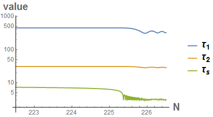
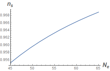
Figure 1: Inflationary evolution of Kähler Moduli Inflation. The inflaton reaches the minimum of the potential at around $N=226$, while inflation ends at around $N=224$.

Now we are ready to solve for the inflationary evolution. We start from the initial point

$$\mathcal{V}_{x}^{(\rm ini)}\sim 2439,\quad x_{2}^{(\rm ini)}\sim 6.263,\quad x_{s}^{(\rm ini)}=1.8,$$ (2.17)

where given the value of $x_{s}$, the directions $\mathcal{V}_{x}$ and $x_{2}$ are stabilized. We impose no initial kick for our analysis. We also have to specify the overall normalization $W_{0}^{2}a_{2}^{3}$ of the potential (2.9) which essentially determines the scale of the power spectrum. Together with a concrete setup of the rank of gauge groups required to generate the non-perturbative terms, we use

$$W_{0}={1\over 68},\quad a_{2}={2\pi\over 31},\quad a_{5}={2\pi\over 2},$$ (2.18)

consistent with $\gamma=15.5$. This initial point satisfies the slow-roll conditions with

$$\begin{split}\epsilon_{\rm ini}\sim 9.026\times 10^{-11},\quad\eta_{\rm ini}\sim-4.544\times 10^{-3},\end{split}$$ (2.19)

where we have used the formula of generalized slow-roll parameters defined in Appendix A. For illustration of our parameter choice, we write down the VEV of the moduli fields before the redefinition used in (2.6). With the value of $a_{2}$, we have

$$\mathcal{V}^{(\rm min)}\sim 16930,\quad\tau_{2}^{(\rm min)}\sim 28.87,\quad\tau_{s}^{(\rm min)}\sim 3.072$$ (2.20)

at the minimum point.

The inflationary trajectory can be solved using the efficient formalism explained in Appendix A starting from the initial point (2.17). The two relevant plots are shown in Figure 1. Inflation ends at $N\sim 224$ where the slow-roll condition breaks down:

$$\epsilon_{\rm end}\sim 8.503\times 10^{-6},\quad\eta_{\rm end}\sim-1.297,$$ (2.21)

and further reaches to the minimum point (2.16) at $N\sim 226$. Note that $N$ is the e-folding number from the initial point, while $N_{e}$ is the e-folding number counted backwards from the end of inflation.

It is worth commenting on the the flatness of the potential. As inflaton is dominantly single field in the $\tau_{s}$ direction for large values of $\tau_{s}$, we crudely approximate the slow-roll parameters by

$$\begin{split}&\epsilon\sim K^{\tau_{s}\tau_{s}}\left({\partial_{\tau_{s}}V\over V}\right)^{2}\propto\mathcal{V}^{3}\tau_{s}^{5/2}e^{-2a_{5}\tau_{s}},\\ &|\eta|\sim K^{\tau_{s}\tau_{s}}\left({\partial_{\tau_{s}}^{2}V\over V}\right)\propto\mathcal{V}^{2}\tau_{s}^{3/2}e^{-a_{5}\tau_{s}},\end{split}$$ (2.22)

where we have used $K^{\tau_{s}\tau_{s}}\propto\mathcal{V}\sqrt{\tau_{s}}$ and the approximated potential in the inflation era given by $V\sim v_{0}/\mathcal{V}^{3}+v_{1}\tau_{s}e^{-a_{5}\tau_{s}}/\mathcal{V}^{2}$ with some constants $v_{0},v_{1}$. Then the small $|\eta_{*}|\ll 1$ evaluated at the CMB point implies

$$\epsilon_{*}\sim\eta_{*}^{2}\mathcal{V}^{-1}\tau_{s}^{-1/2}\ll\mathcal{V}^{-1}\tau_{s}^{-1/2}.$$ (2.23)

So we see that the value of $\epsilon$ is much smaller than $\eta$ at large volume, resulting in a small value of the tensor to scalar ratio $r$.

We now illustrate some observables at a sample point $N_{e}=60$ for a better understanding. Solving the differential equations (A.6) numerically, we obtain

$$\epsilon_{60}\sim 1.302\times 10^{-9},\quad\eta_{60}\sim-0.01702,$$ (2.24)

or correspondingly,

$$n_{s}^{(60)}\sim 0.9660,\quad r^{(60)}\sim 2.08\times 10^{-8}.$$ (2.25)

Also, the magnitude of the primordial curvature perturbation is estimated by

$$P_{s}(k_{60})\sim 2.165\times 10^{-9}.$$ (2.26)

The cosmological values here nicely agree with the recent results of the Planck collaboration [2, 3].

Let us consider the values of the moduli fields at the $N_{e}=60$ point, given by

$$\mathcal{V}_{x}^{(60)}\sim 2439,\quad x_{2}^{(60)}\sim 6.263,\quad x_{s}^{(60)}\sim 1.709,$$ (2.27)

and hence the exponential term of the potential important for inflation becomes quite tiny compared to the volume:

$$e^{-\gamma x_{s}^{(60)}}\sim e^{-26.50}\sim 3.109\times 10^{-12}\ll{\mathcal{V}^{(60)}}^{-1}\sim 3.742\times 10^{-5}.$$ (2.28)

This large suppression of the term of the inflationary potential is related to the known concern of Kähler Moduli Inflation (see e.g. [36, 37]) as there should exist many corrections to the effective 4D supergravity from string theory. For instance, if there exists a string loop correction as D7-branes wraps $\tau_{s}$ (or $\tau_{5}$), we have a correction to the potential of the form: $\delta V\propto g_{s}^{2}\mathcal{V}^{-3}\tau_{s}^{-1/2}$ [42, 43, 44], which may appear significantly larger than the inflation potential term proportional to $\mathcal{V}^{-2}e^{-\gamma x_{s}}$. Once this term dominates over the exponential potential around the inflation era, the slow-roll parameters turn out to be $\epsilon\propto\mathcal{V}\tau_{s}^{-5/2},\ \eta\propto\mathcal{V}\tau_{s}^{-2}$ and violate the flatness of the inflationary potential. Therefore, Kähler Moduli Inflation requires a special suppression of these terms via very small $g_{s}$ to maintain the dominance of F-term potential or a special brane setup which prohibits the existence of the corresponding string loop corrections depending on $\tau_{s}$. Note that a similar value of $\gamma x_{s}^{(60)}\sim 26.5$ is also obtained in the context of Roulette Inflation in [45]. In the next section, we like to suggest another possibility of inflation in the direction of a Kähler modulus where this concern is alleviated by using an accidental point for inflation.

We have analyzed the potential with the kinetic term obtained from (2.1) imposing the D-term constraint (2.5) to make a better comparison with the analysis in the next section. This kinetic term is slightly different from that of the just three moduli model with $\mathcal{V}=(2\tau_{1})^{3/2}-(2\tau_{2})^{3/2}-(2\tau_{3})^{3/2}$, although the effective potential is exactly the same. We have checked that there is no significant difference in the dynamics especially in the observables $n_{s},r$ except for ${\cal O}(1)$ factors of $r$ and the e-folding from the beginning to the end of inflation.

2.3 Accidental Kähler Moduli Inflation

In this section, we will explore the possibility that inflation in the $\tau_{s}$ direction occurs at a point closer to the minimum relative to Kähler Moduli Inflation such that the concern about dangerous loop corrections of $\tau_{s}$ to the dynamics of inflation is relaxed. To realize successful inflation near the minimum in our setup, one has to tune the parameters in order to achieve the desired flatness of the potential. Also, the initial condition have to be such that inflation starts close to this tuned flat point. This inflationary scenario is thus called accidental inflation as this happens accidentally in the sense of a parametric coincidence. An accidental model was proposed in [12], and accidental inflation in string theory is further studied in [14, 30]. Here we will illustrate how accidental inflation occurs in the context of Kähler Moduli Inflation, especially using a racetrack structure.

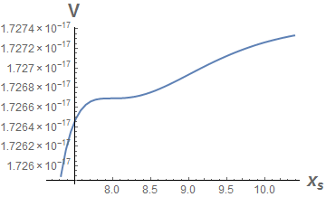
Figure 2: The accidental point for inflation in Accidental Kähler Moduli Inflation. $\mathcal{V}_{x},x_{2}$ are approximately stabilized during inflation.

We use the potential defined in (2.9), but with non-zero $c_{3},c_{4}$ to realize the accidental point. To make a fair comparison, some of the parameters are set to be the same values as in the previous section:

$$\xi_{x}=70,\quad c_{2}=-1,\quad c_{5}=-1.$$ (2.29)

We do not use the large number of the relative ratios of gauge group ranks in the exponent:

$$\alpha=2,\quad\beta=2.1,\quad\gamma=2.2\,.$$ (2.30)

Then the desired accidental point appears when we chose

$$c_{3}=-0.2457004,\quad c_{4}=0.9889189\,.$$ (2.31)

Note that the number of digits we display in (2.31) represents the necessary tuning to realize a flat potential that supports prolonged inflation. The $c_{i}$ parameters depend on the VEVs of the complex structure moduli and the dilaton which in turn are determined by flux quanta. The huge landscape of possible flux vacua leads to the expectation that these parameters can indeed be tuned to high accuracy.

The minimum of the potential is located at Minkowski with a suitable choice of uplift parameter given by

$$d_{x}\sim 3.248\times 10^{-5}\,.$$ (2.32)

Then the minimum sits at

$$\mathcal{V}_{x}^{(\rm min)}\sim 1775,\quad x_{2}^{(\rm min)}\sim 5.976,\quad x_{s}^{(\rm min)}\sim 4.855,$$ (2.33)

where all the eigenvalues of the Hessian are defined positive, such that the moduli are stabilized.

The resultant accidental point is illustrated in Figure 2, where the other moduli are stabilized at

$$\mathcal{V}_{x}^{(\rm acc)}\sim 1785,\quad x_{2}^{(\rm acc)}\sim 5.981,\quad x_{s}^{(\rm acc)}\sim 7.989.$$ (2.34)

Using the general formula of the slow-roll parameters presented in Appendix A, we have

$$\epsilon_{\rm acc}\sim 2.097\times 10^{-11},\quad\eta_{\rm acc}\sim 7.642\times 10^{-6}.$$ (2.35)

The accidental point satisfies the condition $\partial_{x_{s}}^{2}V=0$ by the tuning of $c_{3}$ and $c_{4}$ accordingly. However, $\eta_{\rm acc}$ is not exactly zero due to the presence of off-diagonal entries of both Kähler metric and Hessian together with the fact that the accidental point does not satisfy the extremal condition $\partial_{x_{s}}V=0$. The value of $\epsilon_{\rm acc}$ is small enough to have prolonged inflation.

Interestingly, the values of moduli fields at the accidental point are not so different from not only those at the minimum, but also those in (2.11). Although we construct the model with small $\alpha,\beta,\gamma$, this essentially means that the $x_{s}$ direction turns out to be mostly independent of the other directions owing to the racetrack structure. This feature plays an important role for realizing the accidental point near the minimum.

In the presence of a racetrack potential, one may wonder if the axionic directions are stabilized accordingly, as $c_{4}>0$ contributes as a potential instability at $y_{s}=0$. Given the set of parameters, we have

$$\partial_{y_{2}}^{2}V|_{\rm min}\sim 5.305\times 10^{-14},\quad\partial_{y_{s}}^{2}V|_{\rm min}\sim 3.732\times 10^{-16}\,,$$ (2.36)

at the minimum point, while

$$\partial_{y_{2}}^{2}V|_{\rm acc}\sim 5.218\times 10^{-14},\quad\partial_{y_{s}}^{2}V|_{\rm acc}\sim 1.531\times 10^{-21}\,,$$ (2.37)

at the accidental point. Hence the axionic directions are safely stabilized at $y_{i}=0$ from the beginning to the end of inflation.

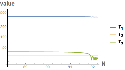
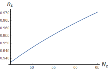
Figure 3: Inflationary evolution of Accidental Kähler Moduli Inflation. The inflaton reaches the minimum of potential at around $N=92$, while inflation ends at around $N=90$.

Now we are ready to solve for the evolution of inflation. We use the accidental point as the initial point. To match the magnitude of the power spectrum with its observed value, we have to specify the overall coefficient of the potential (2.9). This results in the choice

$$W_{0}={1\over 55},\quad a_{2}={2\pi\over 31},$$ (2.38)

where we used the same value of $a_{2}$ as in the previous section. It may be worth rewriting the VEV at the minimum in terms of $\mathcal{V},\tau_{2},\tau_{s}$ by

$$\mathcal{V}^{(\rm min)}\sim 19450,\quad\tau_{2}^{(\rm min)}\sim 29.48,\quad\tau_{s}^{(\rm min)}\sim 23.95.$$ (2.39)

Using the efficient way of solving field evolutions described in Appendix A, the inflaton rolls down the potential as illustrated in Figure 3. The slow-roll condition breaks down at $N\sim 90$ where

$$\epsilon_{\rm end}\sim 7.283\times 10^{-6},\quad\eta_{\rm end}\sim-1.225,$$ (2.40)

and the inflaton starts oscillating around the minimum at $N\sim 92$. Note that we use $N$ for the e-folding from the initial point, while $N_{e}$ for the e-folding from the end of inflation.

At $N_{e}=60$ as a sample point, the slow-roll parameters become

$$\epsilon_{60}\sim 3.356\times 10^{-11},\quad\eta_{60}\sim-0.01847,$$ (2.41)

suggesting

$$n_{s}^{(60)}\sim 0.9631,\quad r^{(60)}\sim 5.369\times 10^{-10}.$$ (2.42)

The values here are not too much different from those in previous section (2.24), although the tensor to scalar ratio $r$ is slightly smaller. The magnitude of the primordial curvature perturbation is given by

$$P(k_{60})\sim 2.202\times 10^{-9}.$$ (2.43)

Thus the values of the observables here again nicely agree with the recent data published by the Planck collaboration [2, 3].

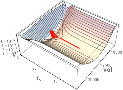
Figure 4: The potential of Accidental Kähler Moduli Inflation at fixed $\tau_{2}$. The red line describes the trajectory of inflation.

The form of potential as well as the inflationary trajectory in $\mathcal{V},\tau_{s}$-space is described in Figure 4. Here we have fixed the $\tau_{2}$ direction as it is approximately constant during inflation.

Finally, let us evaluate the values of the moduli fields at $N_{e}=60$. These are given by

$$\mathcal{V}_{x}^{(\rm 60)}\sim 1785,\quad x_{2}^{(\rm 60)}\sim 5.981,\quad x_{s}^{(\rm 60)}\sim 7.983.$$ (2.44)

Then the exponential suppression in the potential is estimated by

$$e^{-\alpha x_{s}^{(60)}}\sim e^{-15.97}\sim 1.165\times 10^{-7}<{\mathcal{V}^{(\rm 60)}}^{-1}\sim 5.111\times 10^{-5}.$$ (2.45)

When we compare this quantity with the value (2.28) of Kähler Moduli Inflation, we see the significant alleviation of the suppression term while keeping the successful prolonged inflation. This alleviation is important. From the estimation above, we see that each term of the inflationary potential depending on $\tau_{s}$, for instance $\mathcal{V}^{-2}e^{-\alpha x_{s}}$ is larger or comparable to the string-loop correction of the form $\delta V\sim g_{s}^{2}\mathcal{V}^{-3}\tau_{s}^{-1/2}$ with a reasonable value of the string coupling. Therefore we conclude that a slight shift of the moduli fields or of the coefficients can absorb the change induced by the corrections as they appear at the same order or less. This is a feature of Accidental Kähler Moduli Inflation improved by the racetrack structure, that is not achieved in the case of Kähler Moduli Inflation where the correction may appear as the dominant term without a significant suppression by the string coupling or a special brane setup.

It is worth commenting also that this mild suppression is achieved with more realistic ratios of the gauge group ranks $\alpha,\beta,\gamma\sim{\cal O}(1)$, unlike the situation where a large hierarchy in the exponent $\gamma\sim{\cal O}(10)$ or a larger number of small cycles is required in the original Kähler Moduli Inflation. Also, as a by-product, we could take the larger value $x_{s}^{(\rm 60)}\sim 7.983$ or $\tau_{s}\sim 39.39$ as the starting point for the prolonged inflation. This larger value helps a bit to avoid the string-loop correction $\delta V\propto g_{s}^{2}{\cal V}^{-3}\tau_{s}^{-1/2}$ so that the required suppression on $g_{s}$ is alleviated.

One may wonder if the accidental structure of the potential persist in the presence of sub-leading terms in the overall volume in the F-term potential away from the LVS approximation. Although these terms are suppressed by the large volume, it might affect our analysis as the leading potential of ${\cal O}(\mathcal{V}^{-3})$ includes another cancellation due to the racetrack structure for slow-roll inflation at the accidental point. Analyzing the full F-term potential, we see that actually these sub-leading terms do not spoil the existence of both minimum and accidental point. At the accidental point where the additional cancellation works, the structure of the potential consists mostly of $e^{-\alpha x_{s}}/\mathcal{V}_{x},e^{-\beta x_{s}}/\mathcal{V}_{x},e^{-\gamma x_{s}}/\mathcal{V}_{x}$ terms, and the resultant potential changes little in the presence of sub-leading terms. This small change can be easily absorbed by a slight shift of the coefficients $c_{3},c_{4}$ so that a successful phase of prolonged inflation is realized.

3 Ordinary racetrack model

So far we have studied the racetrack model generated through the D-term constraint. In this section, we study the standard racetrack model with triple non-perturbative terms in the superpotential. To be more precise, we consider the following model:

$$\begin{split}&K=-2\ln\left(\mathcal{V}+\xi/2\right),\quad\mathcal{V}=\left(T_{1}+\bar{T}_{1}\right)^{3/2}-\left(T_{2}+\bar{T}_{2}\right)^{3/2}-\left(T_{3}+\bar{T}_{3}\right)^{3/2},\\ &W=W_{0}+A_{2}e^{-a_{2}T_{2}}+A_{3}e^{-a_{3}T_{3}}+B^{(1)}_{3}e^{-b_{3}^{(1)}T_{3}}+B^{(2)}_{3}e^{-b_{3}^{(2)}T_{3}},\end{split}$$ (3.1)

where we have used a slightly different volume form compared to the previous section. In this model, the effective potential is of the same form as in the previous section except for the cross-terms of a racetrack structure as we will see below. We assume that there is no D-term constraint for this model.

We first redefine the parameters to remove the redundancy in the dynamics by

$$\begin{split}&c_{2}={A_{2}\over W_{0}},\quad c_{a}={A_{3}\over W_{0}},\quad c_{b}={B_{3}^{(1)}\over W_{0}}\quad c_{c}={B_{3}^{(2)}\over W_{0}},\\ &\alpha={a_{3}\over a_{2}},\quad\beta={b_{3}^{(1)}\over a_{2}},\quad\gamma={b_{3}^{(2)}\over a_{2}},\quad\xi_{x}=a_{2}^{3/2}\xi,\end{split}$$ (3.2)

and

$$\mathcal{V}_{x}=a_{2}^{3/2}\mathcal{V},\quad x_{i}=a_{2}\tau_{i},\quad y_{i}=a_{2}\theta_{i}.$$ (3.3)

Using the redefined parameters above, the F-term potential $V_{F}=e^{K}(|DW|^{2}-3|W|^{2})$ together with the uplift term of (2.9) becomes

$$\begin{split}{V\over W_{0}^{2}a_{2}^{3}}\sim&{d_{x}\over\mathcal{V}_{x}^{4/3}}+{3\xi_{x}\over 4\mathcal{V}_{x}}+{4e^{-x_{2}}c_{2}x_{2}\over\mathcal{V}_{x}^{2}}\cos y_{2}+{2\sqrt{2}e^{-2x_{2}}c_{2}^{2}\sqrt{x_{2}}\over 3\mathcal{V}_{x}}\\ &+{4e^{-\alpha x_{3}}\alpha c_{a}x_{3}\over\mathcal{V}_{x}^{2}}\cos(\alpha y_{3})+{4e^{-\beta x_{3}}\beta c_{b}x_{3}\over\mathcal{V}_{x}^{2}}\cos(\beta y_{3})+{4e^{-\gamma x_{3}}\gamma c_{c}x_{3}\over\mathcal{V}_{x}^{2}}\cos(\gamma y_{3})\\ &+{2\sqrt{2}e^{-2\alpha x_{3}}\alpha^{2}c_{a}^{2}\sqrt{x_{3}}\over 3\mathcal{V}_{x}}+{2\sqrt{2}e^{-2\beta x_{3}}\beta^{2}c_{b}^{2}\sqrt{x_{3}}\over 3\mathcal{V}_{x}}+{2\sqrt{2}e^{-2\gamma x_{3}}\gamma^{2}c_{c}^{2}\sqrt{x_{3}}\over 3\mathcal{V}_{x}}\\ &+{4\sqrt{2}e^{-(\alpha+\beta)x_{3}}\alpha\beta c_{a}c_{b}\sqrt{x_{3}}\over 3\mathcal{V}_{x}}\cos\left((\alpha-\beta)y_{3}\right)+{4\sqrt{2}e^{-(\beta+\gamma)x_{3}}\beta\gamma c_{b}c_{c}\sqrt{x_{3}}\over 3\mathcal{V}_{x}}\cos\left((\beta-\gamma)y_{3}\right)\\ &+{4\sqrt{2}e^{-(\gamma+\alpha)x_{3}}\gamma\alpha c_{c}c_{a}\sqrt{x_{3}}\over 3\mathcal{V}_{x}}\cos\left((\gamma-\alpha)y_{3}\right).\end{split}$$ (3.4)

The last three cross-terms are typically present in case of a superpotential racetrack model as they show up at ${\cal O}(\mathcal{V}^{-3})$. Again the uplift term motivated by an anti-brane uplift is just a choice and the result does not change crucially if we use a different power of the volume dependence, corresponding to a different uplift mechanism.

Now we solve the dynamics. The parameters responsible for the size of the volume are chosen as

$$\xi_{x}=70,\quad c_{2}=-1,\quad c_{c}=-1,$$ (3.5)

such that we can make a fair comparison to the results in the previous section. Unlike the previous situation in the D-term generated racetrack model, it is difficult to realize the stabilization of $\mathcal{V}_{x},x_{2}$ during a phase of successful prolonged inflation in the $x_{3}$ direction unless having hierarchical values of the coefficients $\alpha,\beta,\gamma$. So we set

$$\alpha=7,\quad\beta=7.1,\quad\gamma=7.2,$$ (3.6)

to illustrate a successful example. With the choice of parameters above, the accidental point is achieved with the remaining parameters being

$$c_{a}=-0.73971879,\quad c_{b}=1.71976665,$$ (3.7)

and the axion directions are stabilized at $y_{i}=0$ as before. We are now ready to determine the Minkowski minimum which demand a parameter value

$$d_{x}\sim 4.086\times 10^{-5}.$$ (3.8)

Then the minimum point sits at

$$\mathcal{V}_{x}^{(\rm min)}\sim 1570,\quad x_{2}^{(\rm min)}\sim 5.866,\quad x_{3}^{(\rm min)}\sim 0.6080,$$ (3.9)

where all the eigenvalues of the Hessian are positive.

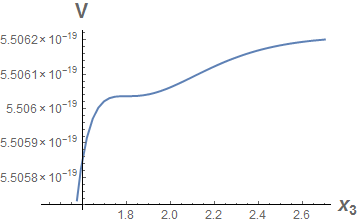
Figure 5: The accidental point for inflation in the ordinary racetrack model. $\mathcal{V}_{x},x_{2}$ are approximately stabilized during inflation.

When we use a smaller choice of $\alpha,\beta,\gamma$, the required value for the uplift $d_{x}$ becomes slightly larger. In fact, this slightly larger value of the uplift parameter is dangerous as this causes a destabilization of the volume direction at larger values of $x_{3}$ where inflation occurs. This is not the case in the D-term generated racetrack model as we have illustrated in Section 2.3, while we have this situation in the ordinary racetrack model. This could be due to the existence of cross-terms appearing in the last three terms of (3.4). We set two of the coefficients $c_{a},c_{b},c_{c}$ to negative values to realize moduli stabilization, suggesting negative entries of the cross-terms at the minimum. To compensate the negative contribution of cross-terms, we have to increase the uplift parameter $d_{x}$. Hence, we have to start with slightly larger values of $\alpha,\beta,\gamma$ to maintain the hierarchy that the cross-term contribution does not violate the stability of $\mathcal{V}_{x},x_{2}$.

With the suitable choice of parameters for our purpose, the accidental point is located at

$$\mathcal{V}_{x}^{(\rm acc)}\sim 2272,\quad x_{2}^{(\rm acc)}\sim 6.199,\quad x_{3}^{(\rm acc)}\sim 1.800,$$ (3.10)

as illustrated in Figure 5 where $\mathcal{V}_{x},x_{2}$ are approximately stabilized. When we use the general expression of slow-roll parameters in Appendix A, we estimate

$$\epsilon_{\rm acc}\sim 6.332\times 10^{-13},\quad\eta_{\rm acc}\sim 6.028\times 10^{-6}.$$ (3.11)

Again, the value of $\eta_{\rm acc}$ is not exactly zero due to the off-diagonal entries and the non-zero value of the first derivative $\partial_{x_{3}}V\neq 0$ although satisfying $\partial_{x_{3}}^{2}V=0$. We will use this accidental point as the initial point for inflation.

Before proceeding, we comment on the stability of the axionic directions as it is not obvious in the racetrack model. At the extremum $y_{i}=0$, there is no mixture of the Hessians between the real and imaginary modes of the moduli fields. The dominant entries of the Hessian of the axionic directions becomes

$$\partial_{y_{2}}^{2}V|_{\rm min}\sim 4.246\times 10^{-17},\quad\partial_{y_{3}}^{2}V|_{\rm min}\sim 1.126\times 10^{-16}$$ (3.12)

at the minimum point and

$$\partial_{y_{2}}^{2}V|_{\rm acc}\sim 1.536\times 10^{-17}.\quad\partial_{y_{3}}^{2}V|_{\rm acc}\sim 1.083\times 10^{-23}$$ (3.13)

at the accidental point. So the axionic directions are indeed stabilized during the entire inflationary evolution.

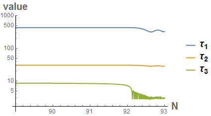
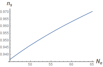
Figure 6: Inflationary evolution in the ordinary racetrack model. The inflaton reaches the minimum of the potential at around $N=93$, while inflation ends at around $N=90$.

Next we discuss the inflationary solution to the field equations (A.6). To fix the overall scale of the potential, we choose

$$W_{0}={1\over 2300},\quad a_{2}={2\pi\over 31},$$ (3.14)

where the value of $a_{2}$ is chosen identical to the previous section to make a fair comparison. With this choice, the values of moduli fields at the minimum are rewritten by

$$\mathcal{V}^{(\rm min)}\sim 17210,\quad\tau_{2}^{(\rm min)}\sim 29.94,\quad\tau_{3}^{(\rm min)}\sim 3.000.$$ (3.15)

Solving by the efficient method described in Appendix A, the slow-roll condition for inflation breaks down at $N\sim 90$ where the slow-roll parameters are estimated as

$$\epsilon_{\rm end}\sim 2.206\times 10^{-7},\quad\eta_{\rm end}\sim-1.123,$$ (3.16)

and the inflaton reaches the minimum at $N\sim 93$. We illustrate the evolution in Figure 6, where $N$ is the e-folding from the initial point and $N_{e}$ is the e-folding from the end of inflation.

Now we estimate some observables at $N_{e}=60$ as a sample point. The slow-roll parameters become

$$\epsilon_{60}\sim 1.071\times 10^{-12},\quad\eta_{60}\sim-0.01874,$$ (3.17)

which implies

$$n_{s}^{(60)}\sim 0.9625,\quad r^{(60)}\sim 1.714\times 10^{-11}.$$ (3.18)

Then the magnitude of the primordial curvature perturbation is estimated as

$$P(k_{60})\sim 2.196\times 10^{-9}.$$ (3.19)

The observables shown here are well in agreement with the recent results of the Planck collaboration [2, 3].

Finally, we present the values of moduli fields for the validity of the approximation. At $N_{e}=60$, the moduli fields have values of

$$\mathcal{V}_{x}^{(60)}\sim 2272,\quad x_{2}^{(60)}\sim 6.199,\quad x_{3}^{(60)}\sim 1.799.$$ (3.20)

Using the values above, we get

$$e^{-\alpha x_{3}^{(60)}}\sim e^{-12.59}\sim 3.405\times 10^{-6}<{\mathcal{V}^{(60)}}^{-1}\sim 4.017\times 10^{-5}.$$ (3.21)

Although we had to choose slightly larger $\alpha,\beta,\gamma$ to maintain an appropriate hierarchy for the stabilization of $\mathcal{V}_{x},x_{2}$, the resultant suppression of the inflation potential is quite alleviated compared to Kähler Moduli Inflation. This is due to the fact that we could start from an initial point near the minimum point, owing to the racetrack structure. Note that the suppression here looks slightly milder than in the case of the D-term generated racetrack model. This could be because we did not try to find an extreme choice of parameters that relaxes the suppression as much as possible. Therefore we consider that the suppressions of the ordinary racetrack model and the D-term generated racetrack model are very similar, and conclude that this alleviation of the suppression is a generic feature of the racetrack models with a suitable accidental point.

Note that the accidental structure persists even in the presence of sub-leading terms in the volume in the F-term potential away from the LVS approximation, similar to Section 2.3. Again, the sub-leading terms change the potential little, and a slight shift of the coefficients $c_{a},c_{b}$ can easily absorb the small changes in the potential. This can be anticipated since the resultant contribution of the inflaton field to the potential (3.21) is actually comparable with that in the D-term generated racetrack model (2.45), where the potential is dominated by single exponent terms even in the presence of a racetrack cancellation.

4 Discussion

We have presented Accidental Kähler Moduli Inflation where inflation occurs around an accidental point realized by a racetrack structure. The observable values obtained, i.e., the magnitude of primordial curvature perturbation, spectral index and tensor-to-scalar ratio are within the observational bounds. The concern that string-loop corrections spoil the flatness of the inflaton potential, which is present in the original Kähler Moduli Inflation model, is alleviated in the Accidental Kähler Moduli Inflation model. Inflation occurs at an accidental point near the minimum, avoiding the exponentially large hierarchy of values of the inflationary potential terms between the inflationary era and the minimum. Hence, the correction term can be absorbed in the inflationary potential accordingly. Similar arguments should apply to other potentially dangerous corrections, making our construction rather robust.

We have presented two types of racetrack models: one uses the D-term generated racetrack structure proposed in [33] and the other consists of the ordinary racetrack structure in the superpotential. Given a set of reasonable parameters in the D-term generated racetrack model, a phase of successful prolonged inflation can be realized by a reasonable ratio of gauge group ranks $a_{\rm inf}/a_{\rm stab}=\alpha,\beta,\gamma\sim{\cal O}(1)$ in the exponents, while the original Kähler Moduli Model demands $a_{\rm inf}/a_{\rm stab}\sim{\cal O}(10)$ to realize a sufficient hierarchy between volume modulus stabilization and inflation. In fact, the possible rank of the gauge groups generating the non-perturbative effects is constrained from above by the consistency with tadpole cancellation and holomorphicity [46, 47, 48], and hence it may not be easy to achieve such large hierarchies of $\gamma\sim{\cal O}(10)$ in explicit models. Also, since the D-term generated racetrack model is constructed with a larger number of Kähler moduli, the maximal gauge group rank satisfying the consistency conditions is actually larger than that of model starting with smaller number of moduli [48]. However, the constraint on $\gamma$ also becomes less severe in the original model of Kähler Moduli Inflation when the number of small cycles increases. To summarize, we consider the D-term generated racetrack model for accidental inflation is realizable in the sense of explicit model constructions in string theory. Note that the ordinary racetrack model requires slightly larger coefficients to maintain the hierarchy, but a phase of prolonged inflation is realized with $a_{\rm inf}/a_{\rm stab}<10$ and thus is reasonable too.

Although the realization of the accidental point requires the tuning of coefficients and initial conditions, it does not require unnatural hierarchies of the coefficients $c_{i}=A_{i}/W_{0}$. The coefficient of each racetrack term is determined by the stabilization of the complex structure moduli and dilaton, and hence we expect that the coefficients appear at the same order of magnitude in general, which is actually the case for the models considered in this paper.

The racetrack structure can be realized without unacceptable differences of ratios $\alpha,\beta,\gamma$ in the exponents. The difference of $(\beta-\alpha)\sim{\cal O}(10^{-1})$ etc. is easily realized by taking slightly different gauge group ranks of D7-branes wrapping the inflationary cycle. Although we used that each ratio differed by ‘0.1’ as an illustration throughout this paper, the system works even with larger differences. In addition, for the D-term generated racetrack model, the D-term constraint may be generalized to be $\tau_{3}=\delta_{4}\cdot\tau_{4}=\delta_{5}\cdot\tau_{5}$ with a more complicated configuration of magnetic flux on D7-branes associated with the D-terms, where $\delta_{4},\delta_{5}\neq 1$ are some rational numbers. This different choice of D-term constraints affects the ratios $\alpha,\beta,\gamma$ in the exponents, and hence it certainly helps to realize even smaller differences of ratios, resulting in a better racetrack with less tuning of coefficients $c_{i}$ of each racetrack term. Another advantage of the D-term generated racetrack model is that we do not need to worry about the detailed physics related to the split of gauge group ranks which would be required to realize the ordinary racetrack terms in the superpotential.

Even though the existence of an inflection point is conceivable in a complicated string moduli space, one may worry about the overshooting problem of initial conditions. When we start from a higher point along the inflationary direction, more e-folds are achieved since the potential around the inflection point is flat enough. However, given the values of coefficients ($A_{i},W_{0}$), the resultant spectral index at CMB point differs from the observational value with the different initial condition. If we were to allow changing the values of the coefficients simultaneously with the initial condition, some region in the parameter space would be allowed. Although there is a discussion of this issue in the context of string theory [49, 31], we hope to report more on this issue in the future.

One may worry about isocurvature perturbations which are currently severely constrained by the Planck collaboration [2, 3]. The light mode contributing to isocurvature perturbations is regarded as a massless particle during inflation. In our model this is the axionic partner of the overall volume modulus. The other fields are heavy enough and hence the adiabatic perturbations are essentially driven by the single inflaton field. The mass of $\theta_{1}$ is generated by a non-perturbative effect on $T_{1}$, that is sub-dominant in LVS and we did not specify in our model. If the mass scale is large enough to be a dark matter, this axion also contributes to the CDM isocurvature perturbations. Since the magnitude of CDM isocurvature perturbation crucially depends on the initial mis-alignment angle and the fraction of CDM consisting of axion, we believe that the CDM isocurvature constraint is satisfied (see e.g. Figure 6 of [50] at $H_{\rm inf}\sim 10^{10}\ {\rm GeV},\ f_{a}\sim 10^{16}\ {\rm GeV}$ of our illustrative example). On the other hand, when the mass scale is negligible even at the minimum of LVS, this lightest axion could play a role of dark radiation. In this case, although the direct entropy production from axion perturbations would not be subject to the constraint as the axion only has derivative couplings and hence the entropy is diluted away quickly, the dark radiation produced by the decay of the volume modulus may contribute to the neutrino isocurvature density perturbations [51]. However, a more conclusive discussion requires more details of the setup including the location of the matter sector in the compact manifold. Hence, we consider this is beyond the scope of the paper.

So far, we have focused on accidental inflation which occurs near an inflection point. It may be interesting to see what happens when inflation starts near a saddle point instead, as studied in [52, 53]. Although axionic saddle points were used in [52, 53], when inflation occurs along the small modulus direction, two racetrack terms may be able to form a saddle point in the small modulus direction. However, not only $\epsilon$, but also $\eta$ needs to be suppressed for successful inflation. To realize this, we may need an additional racetrack term or other contributions to the potential. Saddle point inflation along the small modulus direction also needs the correct initial conditions that the inflaton does not roll down a runaway direction which would result in decompactification. We hope to pursue this direction in the future.

Appendix A Slow-roll parameters and dynamics

In this appendix, we denote the details of the inflationary dynamics as well as the definition of the slow-roll parameters. We follow the efficient way of solving the full set of equations of motions for the inflationary trajectories used in [53].

First, the kinetic term is written by

$${\cal L}_{\rm kin}={\partial^{2}K\over\partial T_{I}\bar{T}_{J}}\partial_{\mu}T_{I}\partial^{\mu}\bar{T}_{J}=-{1\over 2}g_{ab}\partial_{\mu}\phi^{a}\partial^{\mu}\phi^{b},$$ (A.1)

where $T_{I}=T_{1},T_{2},T_{3},T_{4},T_{5}$ and $\phi^{a}=\tau_{1},\tau_{2},\tau_{s},\theta_{2},\theta_{s}$ in the D-term generated racetrack model of Section 2. Note that we have imposed the D-term constraint (2.5) in the second equation, and have neglected $\theta_{1}$. We use a different coordinate system accordingly in the ordinary racetrack model of Section 3. Using the non-canonical metric, the generalized slow-roll parameters are defined by

$$\epsilon={1\over 2}g^{ab}{\partial_{a}V\partial_{b}V\over V^{2}},$$ (A.2)

and the most negative eigenvalue of the matrix

$$N^{a}_{\ b}=g^{ac}{\partial_{c}\partial_{b}V-\Gamma^{d}_{cb}\partial_{d}V\over V}$$ (A.3)

gives the other slow-roll parameter $\eta$. $\Gamma^{d}_{cb}$ is the connection obtained form $g_{ab}(\phi)$ in the normal fashion. It may also be convenient to write down the slow-roll parameters in terms of the complex coordinates:

$$\begin{split}&\epsilon=K^{I\bar{J}}{\partial_{I}V\partial_{\bar{J}}V\over V^{2}},\qquad N^{a}_{\ b}=\left(\begin{array}[]{cc}N^{I}_{\ J}&N^{I}_{\ \bar{J}}\\ N^{\bar{I}}_{\ J}&N^{\bar{I}}_{\ \bar{J}}\end{array}\right),\\ &N^{I}_{\ J}=K^{I\bar{K}}{\partial_{\bar{K}}\partial_{J}V\over V},\quad N^{I}_{\ \bar{J}}=K^{I\bar{K}}{\partial_{\bar{J}}\partial_{\bar{K}}V-K^{L\bar{M}}\partial_{\bar{J}}\partial_{\bar{K}}\partial_{L}K\partial_{\bar{M}}V\over V}.\end{split}$$ (A.4)

Note that $N^{\bar{I}}_{\ \bar{J}},N^{\bar{I}}_{\ J}$ are complex conjugate of $N^{I}_{\ J},N^{I}_{\ \bar{J}}$.

The inflationary evolution can be calculated efficiently when we introduce the canonical momenta defined by

$$\begin{split}\pi_{a}={\partial{\cal L}_{\rm kin}\over\partial\dot{\phi}^{a}}.\end{split}$$ (A.5)

Using these equations, we solve $\dot{\phi}^{a}$ as functions of $\pi_{a}$. Then the equation of motions become

$$\begin{split}{d\phi^{a}\over dN}=&{1\over H}\dot{\phi}^{a}(\pi),\\ {d\pi_{a}\over dN}=&-3\pi_{a}-{1\over H}{\partial\over\partial\phi^{a}}\left(V-{\cal L}_{\rm kin}\right),\\ 3H^{2}=&\rho={\cal L}_{\rm kin}+V,\end{split}$$ (A.6)

where $N$ is the number of e-foldings from the initial point of inflation. As explained in [53], we can avoid computing Christoffel symbols directly in field space owing to the introduction of the canonical momenta $\pi_{a}$, and hence save some computational cost.

We may approximate the equations of motion (A.6) under the slow-roll approximation. When the inflation trajectory is well approximated by a single field and the other fields are stabilized, the equation becomes

$$3H^{2}{d\phi^{\rm i}\over dN}+g^{ii}\partial_{i}V=0,$$ (A.7)

where $i$ denotes the direction of inflation, which is $\tau_{s}$ or $\tau_{3}$ in the models we consider. This approximate equation suggests

$$N_{e}\sim\int_{\phi^{i}_{\rm end}}^{\phi^{i}_{\rm CMB}}d\phi^{i}{V\over g^{ii}\partial_{i}V},$$ (A.8)

where $N_{e}$ is the e-folding from the end of inflation and we have used values at the end of inflation $\phi^{i}_{\rm end}$ and at the CMB point $\phi^{i}_{\rm CMB}$. In the accidental scenario we study in this paper, all values of $N,N_{e}$ are estimated by solving the full equations of motion (A.6), while the equation under the slow-roll approximation gives mostly the same results except for a few small numerical differences.

The power spectrum of adiabatic scalar density perturbations under the slow-roll condition is estimated by

$$P_{s}(k)={1\over 8\pi^{2}}{H^{4}\over{\cal L}_{\rm kin}}\sim{1\over 24\pi^{2}}{V\over\epsilon},$$ (A.9)

which is evaluated at the horizon crossing point $k=aH\sim He^{N}$. Therefore the spectral index becomes

$$n_{s}-1={d\ln P_{s}(k)\over d\ln k}\sim{d\ln P_{s}(N)\over dN}\sim 2\eta-6\epsilon.$$ (A.10)

Finally, the tensor to scalar ratio is given by

$$r={P_{t}(k)\over P_{s}(k)}\sim 16\epsilon.$$ (A.11)

References

- [1] G. Hinshaw et al., “Nine-Year Wilkinson Microwave Anisotropy Probe (WMAP) Observations: Cosmological Parameter Results,” Astrophys.J.Suppl. 208 (2013) 19, arXiv:1212.5226 [astro-ph.CO].
- [2] Planck Collaboration, P. Ade et al., “Planck 2015 results. XX. Constraints on inflation,” arXiv:1502.02114 [astro-ph.CO].
- [3] Planck Collaboration Collaboration, P. Ade et al., “Planck 2015 results. XIII. Cosmological parameters,” arXiv:1502.01589 [astro-ph.CO].
- [4] BICEP2, Planck Collaboration, P. Ade et al., “Joint Analysis of BICEP2/ and Data,” Phys.Rev.Lett. 114 (2015) no. 10, 101301, arXiv:1502.00612 [astro-ph.CO].
- [5] P. Creminelli, D. L. Nacir, M. Simonovic, G. Trevisan, and M. Zaldarriaga, “Detecting Primordial -Modes after Planck,” arXiv:1502.01983 [astro-ph.CO].
- [6] T. Matsumura, Y. Akiba, J. Borrill, Y. Chinone, M. Dobbs, et al., “Mission design of LiteBIRD,” arXiv:1311.2847 [astro-ph.IM].
- [7] E. Silverstein, “Les Houches lectures on inflationary observables and string theory,” arXiv:1311.2312 [hep-th].
- [8] F. Quevedo, “Local string models and moduli stabilisation,” Mod.Phys.Lett. A30 (2015) 1530004, arXiv:1404.5151 [hep-th].
- [9] D. Baumann and L. McAllister, “Inflation and String Theory,” arXiv:1404.2601 [hep-th].
- [10] S. B. Giddings, S. Kachru, and J. Polchinski, “Hierarchies from fluxes in string compactifications,” Phys.Rev. D66 (2002) 106006, arXiv:hep-th/0105097.
- [11] K. Dasgupta, G. Rajesh, and S. Sethi, “M theory, orientifolds and G - flux,” JHEP 9908 (1999) 023, arXiv:hep-th/9908088 [hep-th].
- [12] R. Holman, P. Ramond, and G. G. Ross, “Supersymmetric Inflationary Cosmology,” Phys.Lett. B137 (1984) 343–347.
- [13] D. H. Lyth and A. Riotto, “Particle physics models of inflation and the cosmological density perturbation,” Phys.Rept. 314 (1999) 1–146, arXiv:hep-ph/9807278 [hep-ph].
- [14] A. D. Linde and A. Westphal, “Accidental Inflation in String Theory,” JCAP 0803 (2008) 005, arXiv:0712.1610 [hep-th].
- [15] S. Kachru, R. Kallosh, A. D. Linde, J. M. Maldacena, L. P. McAllister, et al., “Towards inflation in string theory,” JCAP 0310 (2003) 013, hep-th/0308055.
- [16] G. Dvali and S. H. Tye, “Brane inflation,” Phys.Lett. B450 (1999) 72–82, arXiv:hep-ph/9812483 [hep-ph].
- [17] S. H. Alexander, “Inflation from D - anti-D-brane annihilation,” Phys.Rev. D65 (2002) 023507, arXiv:hep-th/0105032 [hep-th].
- [18] G. Dvali, Q. Shafi, and S. Solganik, “D-brane inflation,” arXiv:hep-th/0105203 [hep-th].
- [19] C. Burgess, M. Majumdar, D. Nolte, F. Quevedo, G. Rajesh, et al., “The Inflationary brane anti-brane universe,” JHEP 0107 (2001) 047, arXiv:hep-th/0105204 [hep-th].
- [20] D. Choudhury, D. Ghoshal, D. P. Jatkar, and S. Panda, “Hybrid inflation and brane - anti-brane system,” JCAP 0307 (2003) 009, arXiv:hep-th/0305104 [hep-th].
- [21] D. Baumann, A. Dymarsky, I. R. Klebanov, J. M. Maldacena, L. P. McAllister, et al., “On D3-brane Potentials in Compactifications with Fluxes and Wrapped D-branes,” JHEP 0611 (2006) 031, arXiv:hep-th/0607050 [hep-th].
- [22] D. Baumann, A. Dymarsky, S. Kachru, I. R. Klebanov, and L. McAllister, “Holographic Systematics of D-brane Inflation,” JHEP 0903 (2009) 093, arXiv:0808.2811 [hep-th].
- [23] D. Baumann, A. Dymarsky, S. Kachru, I. R. Klebanov, and L. McAllister, “D3-brane Potentials from Fluxes in AdS/CFT,” JHEP 1006 (2010) 072, arXiv:1001.5028 [hep-th].
- [24] D. Baumann, A. Dymarsky, I. R. Klebanov, L. McAllister, and P. J. Steinhardt, “A Delicate universe,” Phys.Rev.Lett. 99 (2007) 141601, arXiv:0705.3837 [hep-th].
- [25] A. Krause and E. Pajer, “Chasing brane inflation in string-theory,” JCAP 0807 (2008) 023, arXiv:0705.4682 [hep-th].
- [26] D. Baumann, A. Dymarsky, I. R. Klebanov, and L. McAllister, “Towards an Explicit Model of D-brane Inflation,” JCAP 0801 (2008) 024, arXiv:0706.0360 [hep-th].
- [27] N. Agarwal, R. Bean, L. McAllister, and G. Xu, “Universality in D-brane Inflation,” JCAP 1109 (2011) 002, arXiv:1103.2775 [astro-ph.CO].
- [28] L. McAllister, S. Renaux-Petel, and G. Xu, “A Statistical Approach to Multifield Inflation: Many-field Perturbations Beyond Slow Roll,” JCAP 1210 (2012) 046, arXiv:1207.0317 [astro-ph.CO].
- [29] H.-Y. Chen, L.-Y. Hung, and G. Shiu, “Inflation on an Open Racetrack,” JHEP 0903 (2009) 083, arXiv:0901.0267 [hep-th].
- [30] I. Ben-Dayan, S. Jing, A. Westphal, and C. Wieck, “Accidental inflation from Kähler uplifting,” JCAP 1403 (2014) 054, arXiv:1309.0529 [hep-th].
- [31] J. J. Blanco-Pillado, M. Gomez-Reino, and K. Metallinos, “Accidental Inflation in the Landscape,” JCAP 1302 (2013) 034, arXiv:1209.0796 [hep-th].
- [32] J. P. Conlon, R. Kallosh, A. D. Linde, and F. Quevedo, “Volume Modulus Inflation and the Gravitino Mass Problem,” JCAP 0809 (2008) 011, arXiv:0806.0809 [hep-th].
- [33] M. Rummel and Y. Sumitomo, “De Sitter Vacua from a D-term Generated Racetrack Uplift,” JHEP 1501 (2015) 015, arXiv:1407.7580 [hep-th].
- [34] V. Balasubramanian, P. Berglund, J. P. Conlon, and F. Quevedo, “Systematics of moduli stabilisation in Calabi-Yau flux compactifications,” JHEP 0503 (2005) 007, hep-th/0502058.
- [35] J. P. Conlon and F. Quevedo, “Kahler moduli inflation,” JHEP 0601 (2006) 146, arXiv:hep-th/0509012 [hep-th].
- [36] M. Cicoli, C. Burgess, and F. Quevedo, “Fibre Inflation: Observable Gravity Waves from IIB String Compactifications,” JCAP 0903 (2009) 013, arXiv:0808.0691 [hep-th].
- [37] C. Burgess, M. Cicoli, and F. Quevedo, “String Inflation After Planck 2013,” JCAP 1311 (2013) 003, arXiv:1306.3512 [hep-th].
- [38] K. Becker, M. Becker, M. Haack, and J. Louis, “Supersymmetry breaking and alpha-prime corrections to flux induced potentials,” JHEP 0206 (2002) 060, hep-th/0204254.
- [39] M. Haack, D. Krefl, D. Lust, A. Van Proeyen, and M. Zagermann, “Gaugino Condensates and D-terms from D7-branes,” JHEP 0701 (2007) 078, arXiv:hep-th/0609211 [hep-th].
- [40] S. Kachru, J. Pearson, and H. L. Verlinde, “Brane / flux annihilation and the string dual of a nonsupersymmetric field theory,” JHEP 0206 (2002) 021, arXiv:hep-th/0112197.
- [41] S. Kachru, R. Kallosh, A. D. Linde, and S. P. Trivedi, “De Sitter vacua in string theory,” Phys.Rev. D68 (2003) 046005, arXiv:hep-th/0301240.
- [42] M. Berg, M. Haack, and E. Pajer, “Jumping Through Loops: On Soft Terms from Large Volume Compactifications,” JHEP 0709 (2007) 031, arXiv:0704.0737 [hep-th].
- [43] M. Cicoli, J. P. Conlon, and F. Quevedo, “General Analysis of LARGE Volume Scenarios with String Loop Moduli Stabilisation,” JHEP 0810 (2008) 105, arXiv:0805.1029 [hep-th].
- [44] M. Cicoli, J. P. Conlon, and F. Quevedo, “Systematics of String Loop Corrections in Type IIB Calabi-Yau Flux Compactifications,”JHEP 0801 (Aug., 2008) 052, 0708.1873.
- [45] J. R. Bond, L. Kofman, S. Prokushkin, and P. M. Vaudrevange, “Roulette inflation with Kahler moduli and their axions,” Phys.Rev. D75 (2007) 123511, arXiv:hep-th/0612197 [hep-th].
- [46] A. Collinucci, F. Denef, and M. Esole, “D-brane Deconstructions in IIB Orientifolds,” JHEP 0902 (2009) 005, arXiv:0805.1573 [hep-th].
- [47] M. Cicoli, C. Mayrhofer, and R. Valandro, “Moduli Stabilisation for Chiral Global Models,” JHEP 1202 (2012) 062, arXiv:1110.3333 [hep-th].
- [48] J. Louis, M. Rummel, R. Valandro, and A. Westphal, “Building an explicit de Sitter,” JHEP 1210 (2012) 163, arXiv:1208.3208 [hep-th].
- [49] N. Itzhaki and E. D. Kovetz, “Inflection Point Inflation and Time Dependent Potentials in String Theory,” JHEP 0710 (2007) 054, arXiv:0708.2798 [hep-th].
- [50] M. Kawasaki, K. Nakayama, T. Sekiguchi, T. Suyama, and F. Takahashi, “Non-Gaussianity from isocurvature perturbations,” JCAP 0811 (2008) 019, arXiv:0808.0009 [astro-ph].
- [51] M. Kawasaki, K. Miyamoto, K. Nakayama, and T. Sekiguchi, “Isocurvature perturbations in extra radiation,” JCAP 1202 (2012) 022, arXiv:1107.4962 [astro-ph.CO].
- [52] J. Blanco-Pillado, C. Burgess, J. M. Cline, C. Escoda, M. Gomez-Reino, et al., “Racetrack inflation,” JHEP 0411 (2004) 063, arXiv:hep-th/0406230 [hep-th].
- [53] J. Blanco-Pillado, C. Burgess, J. M. Cline, C. Escoda, M. Gomez-Reino, et al., “Inflating in a better racetrack,” JHEP 0609 (2006) 002, arXiv:hep-th/0603129 [hep-th].