Leptonic CP Violation from a New Perspective

Abstract

We study leptonic CP violation from a new perspective. For Majorana neutrinos, a new parametrization for leptonic mixing of the form $V=O_{23}\,O_{12}\,K_{a}^{i}\cdot O$ reveals interesting aspects that are less clear in the standard parametrization. We identify several important scenario-cases with mixing angles in agreement with experiment and leading to large leptonic CP violation. If neutrinos happen to be quasi-degenerate, this new parametrization might be very useful, e.g., in reducing the number of relevant parameters of models.

I Introduction

Observations of neutrino oscillations have solidly established the massiveness of the neutrinos and the existence of leptonic mixing. Since neutrinos are strictly massless in the standard model (SM), these observations require necessarily new physics beyond the SM. One is still far from a complete picture of the lepton sector, i.e., many fundamental questions need to be answered. Not only the origin of the leptonic flavor structure remains unknown, but leptonic mixing differs tremendously from the observed quark mixing. Moreover, the absolute neutrino mass scale is still missing, one does not know whether neutrinos are Majorana or Dirac particles, and the nature of leptonic CP violation is still open (for a recent review see Ref. Branco et al. (2012a)).

During the last decades, several attempts were made in order to overcome these fundamental questions. In particular, one may impose family symmetries forbidding certain couplings and at the same time explaining successfully the observed structure of masses and mixings, as well as predicting some other observables King et al. (2014); Shimizu and Tanimoto (2015); Wang et al. (2013); King and Luhn (2013); Boucenna et al. (2012); Ferreira et al. (2012); Branco et al. (2012b); Hernandez and Smirnov (2013a); Eby and Frampton (2012); Ge et al. (2012); Toorop et al. (2011); Zhou (2011); Altarelli and Feruglio (2010); Datta et al. (2005). Although the structure of leptonic mixing is predicted in such models, the mass spectrum turns out to be unconstrained by such symmetries. The connection of leptonic mixing angles and CP-phases with neutrino spectra in the context of partially and completely degenerate neutrinos was proposed in Hernandez and Smirnov (2013b). In an alternative approach, the anarchy of the leptonic parameters is assumed so that there is no physical distinction among three generations of lepton doublets Hall et al. (2000); Haba and Murayama (2001); de Gouvea and Murayama (2003); Altarelli et al. (2012).

From the analysis of neutrino oscillation experiments one can extract bounds for the light neutrino mass square differences $\Delta m_{21}^{2}\equiv m_{2}^{2}-m_{1}^{2}$ and $\Delta m_{31}^{2}\equiv m_{3}^{2}-m_{1}^{2}$. All knowledge on the light neutrino mixing is encoded in the Pontecorvo-Maki-Nakagawa-Sakata matrix (PMNS) Pontecorvo (1957); Maki et al. (1962); Pontecorvo (1968). In order to further analyze the leptonic flavour structure, it is essential to parametrize all the entries of the full PMNS matrix in terms of six independent parameters. It is clear that the choice of a parametrization does not impose any constraints on the physical observables. However, parametrizations are an important tool to interpret underlying symmetries or relations that the data may suggest. In this sense, different parametrizations are certainly equivalents among themselves, although some particular patterns indicated by the data are easer to visualize in some parametrizations than in others. Moreover, special limits suggested by some parametrizations are obfuscated in others.

Among many parametrization proposed in the literature, the standard parametrization is the most widely used, and the six parameters are three mixing angles, namely $\theta_{12},\,\theta_{13}\,,\theta_{23}\in[0,\pi/2]$, one Dirac-type phase $\delta$ and two Majorana phases $\alpha_{1},\alpha_{2}$ in following form:

$$V^{SP}\,=\,K\cdot O_{23}\cdot K_{D}\cdot O_{13}\cdot O_{12}\cdot K_{M}\,,$$ (1)

where the real orthogonal matrices $O_{12}$, $O_{13}$ and $O_{23}$ are the usual rotational matrices in the $(1,2)-$, $(1,3)-$, and $(2,3)-$sector, respectively. The diagonal unitary matrices $K_{D}$ and $K_{M}$ are given by $K_{D}\equiv\operatorname{diag}(1,1,e^{i\alpha_{D}})$ and $K_{M}\equiv\operatorname{diag}(1,e^{i\alpha_{1}^{M}},e^{i\alpha_{2}^{M}})$. Within the standard parametrization, one may recall that the consistent values for the neutrino mixing angles $\theta_{12}$ and $\theta_{23}$ together with the smallness of $\theta_{13}$ suggest that the neutrino mixing is rather close to the tribimaximal mixing (TBM) Harrison et al. (2002). It is important to stress that this parametrization is (modulo irrelevant phases), the same as the one used for the quark sector, despite the fact of leptonic mixing being quite different.

In this paper we study leptonic CP Violation in the context of a new parametrization for leptonic mixing of the form

$$V\,=\,O_{23}\,O_{12}\,K_{\alpha}^{i}\cdot O\,,$$ (2)

where $O$ is a real orthogonal matrix parametrized with three mixing angles. This new parametrization turns out to be very useful in the case where neutrinos are quasi-degenerate Majorana fermions Branco et al. (1999a). It may reflect some specific nature of neutrinos, suggesting that there is some major intrinsic Majorana character of neutrino mixing and CP violation present in the left part of the parametrization, while the right part, in the form of the orthogonal matrix $O$, may reflect the fact that there are 3 neutrino families with small mass differences and results in small mixings. Thus, the intrinsic Majorana character of neutrinos may be large with a large contribution to neutrino mixing (from some yet unknown source), while the extra mixing $O$ of the families is comparable to the quark sector and may be small, of the order of the Cabibbo angle.

The new parametrization permits a new view of large leptonic CP Violation. It reveals interesting aspects that are less clear in the standard parametrization. We identify five scenario-cases that lead to large Dirac-CP violation, and which have mixing angles in agreement with experimental data. A certain scenario (I-A) is found to be the most appealing, since it only needs 2 parameters to fit the experimental results on lepton mixing and provides large Dirac-CP violation and large values for the Majorana-CP violating phases.

The paper is organized as follows. In the next section, we prove the consistency of the new parametrization stated in Eq. (2). In Sec. III, we motivate the use of this new parametrization in the limit of degenerate or quasi-degenerate neutrino spectrum. Then in Sec. IV, we present an alternative view of large leptonic CP violation, using the new parametrization for leptonic mixing, discuss its usefulness and identify several important scenario-cases. Results are shown for mixing and CP violation. In Sec. V, we give a numerical analysis of the scenarios described in the previous section, and, for the quasi-degenerate Majorana neutrinos, a numerical analysis of their stability. Finally, in Sec. VI, we present our conclusions.

II A novel parametrization

In this section, we present the new parametrization for the lepton mixing matrix. First, we prove that any unitary matrix can be written with the following structure:

$$V\,=K_{S}\,\ O_{23}\,O_{12}\ K_{\alpha}^{i}\cdot O\,,$$ (3)

where $K_{S}\,=\operatorname{diag}(e^{i\alpha_{1}},e^{i\alpha_{2}},e^{i\alpha_{3}})$ is a pure phase unitary diagonal matrix, $O_{23},$ $O_{12}$ are two elementary orthogonal rotations in the $(23)$- and $(12)$-planes, $K_{\alpha}^{i}=\operatorname{diag}(1,i,e^{i\alpha})$ has just one complex phase $\alpha$ (apart from the imaginary unit $i$), and $O$ is a general orthogonal real matrix described by 3 angles.

Proof: Let us start from a general unitary matrix $V$ and compute the following symmetric unitary matrix $S$,

$$S\,=\,V^{\ast}\,V^{\dagger}\,.$$ (4)

Assuming that $S\,$ is not trivial, i.e. it is not a diagonal unitary matrix, one can rewrite the matrix $S$ as

$$S\,=\,K_{S}^{\ast}\,\,\ S_{0}\,\ K_{S}^{\ast}\,,$$ (5)

with a pure phase diagonal unitarymatrix $K_{S}=\operatorname{diag}(e^{i\alpha_{1}},e^{i\alpha_{2}},e^{i\alpha_{3}})$ so that the first row and the first column of $S_{0}$ become real. In fact, the diagonal matrix $K_{S}$ has no physical meaning, since it only rephases the PMNS matrix $V$ on the left. This can be clearly seen in the weak basis where the charged lepton mass matrix is diagonal and through a weak basis transformation the phases in $K_{S}$ can be absorbed by the redefinition of the right-handed charged lepton fields. One can now perform a $(23)-$rotation on $S_{0}$ as,

$$S_{0}^{\prime}\,=\,O_{23}^{\intercal}\,S_{0}\,O_{23}\,,$$ (6)

with a orthogonal matrix $O_{23}$ given by

$$O_{23}\,=\,\begin{pmatrix}1&0&0\\ 0&\cos\theta_{23}&\sin\theta_{23}\\ 0&-\sin\theta_{23}&\cos\theta_{23}\end{pmatrix}\,,$$ (7)

so that the $(13)-$ and $(31)-$elements of the resulting matrix vanish. Making use of unitarity conditions one concludes that automatically the $(13)-$ and $(31)-$elements become also zero and therefore the $(12)-$sector of $S_{0}^{\prime}$ decouples and one obtains that

$$S_{0}\,=\,O_{23}\,O_{12}\cdot\operatorname{diag}(1,-1,e^{-2i\alpha})\cdot O_{12}^{\intercal}\,O_{23}^{\intercal}\,,$$ (8)

where $O_{12}$ is given by

$$O_{12}\,=\,\begin{pmatrix}\cos\theta_{12}&\sin\theta_{12}&0\\ -\sin\theta_{12}&\cos\theta_{12}&0\\ 0&0&1\end{pmatrix}\,.$$ (9)

The matrix $S_{0}$ is then written as

$$S_{0}\,=\,U_{0}^{\ast}\,U_{0}^{\dagger}\,,$$ (10)

where the unitary matrix $U_{0}$ is given by

$$U_{0}\,=\,O_{23}\,O_{12}\,K_{\alpha}^{i}\,,$$ (11)

with $K_{\alpha}^{i}=\operatorname{diag}(1,i,e^{i\alpha})$. Thus, given $V$, we can compute explicitly the matrices $K_{S}$, $O_{23}$, $O_{12}$ and $K_{\alpha}^{i}$. In order to obtain the form given in Eq. (3), we factorize the leptonic mixing $V$ as

$$V\,=\,(K_{S}\,U_{0})\,W_{0}^{\ast}\,,$$ (12)

and we demonstrate that $W_{0}$ is real and orthogonal. By definition, the matrix $W_{0}$,

$$W_{0}\,\equiv\,\left(U_{0}^{\intercal}\ K_{S}\right)\cdot V^{\ast}\,,$$ (13)

is obviously unitary since it is the product of unitary matrices. Let us then verify that $W_{0}$ is indeed orthogonal by computing the product

$$\begin{split}W_{0}\cdot W_{0}^{\intercal}&=\left(U_{0}^{\intercal}\,K_{S}\right)\cdot V^{\ast}\ V^{\dagger}\cdot\left(K_{S}\,U_{0}\right)\\ &=U_{0}^{\intercal}\,K_{S}\,\ S\,\ K_{S}\ U_{0}\,,\end{split}$$ (14)

where we have used Eq. (4). Inserting into this expression the other expression for $S$ given in Eq. (5),and making use of Eq. (10) we find

$$W_{0}\cdot W_{0}^{\intercal}=\mathbbm{1}\,,$$ (15)

which means that $W_{0}$ is real and orthogonal. We thus write $W_{0}$ explicitly as

$$W_{0}\equiv\left(U_{0}^{\intercal}\,K_{S}\right)\cdot V^{\ast}\equiv O\,,$$ (16)

where the $O$ stands for the fact that it is an real-orthogonal matrix. Finally, rewriting this equation, we find for the general unitary matrix $V$

$$V\,=\,K_{S}\cdot U_{0}\cdot O\,,$$ (17)

or with Eq. (11)

$$V\,=\,K_{S}\cdot O_{23}\,O_{12}\,K_{\alpha}^{i}\cdot O\,.$$ (18)

We have thus derived a new parametrization for the lepton mixing matrix, i.e.,

$$V\,=\,O_{23}\,O_{12}\,K_{\alpha}^{i}\cdot O\,,$$ (19)

where we have discarded the unphysical pure phase matrix $K_{S}$. It is clear that, as with the standard parametrization in Eq. (1), this parametrization has also 6 physical parameters, but, some are now of a different nature: 2 angles in $O_{23}$ and $O_{12}$, 3 other angles in $O$, but just one complex phase $\alpha$ in $K_{\alpha}^{i}$. From now on, we use explicitly the following full notation

$$V\,=\,O_{23}^{L}\,O_{12}^{L}\,\cdot K_{\alpha}^{i}\cdot O_{23}^{R}\,O_{13}^{R}\,O_{12}^{R}\,,$$ (20)

where we have identified each of the elementary orthogonal rotations, either on the left or on the right of the CP-violating pure phase matrix $K_{\alpha}^{i}$, with a notation superscript $L,R$.

II.0.1 Other parametrizations

For completeness, we point out, following a similar procedure outlined here, that one can also obtain other forms (from the one in Eqs. (19) and (20)) for the parametrization of the lepton mixing matrixSilva-Marcos (2002). E.g. one can have a parametrization where $V=O_{23}\,O_{13}\,K_{i}^{\alpha}\cdot O$, with $K_{i}^{\alpha}=\operatorname{diag}(1,e^{i\alpha},i)$, or even other variations such as $V=O_{12}\,O_{23}\,\widetilde{K}_{i}^{\alpha}\cdot O$, with $\widetilde{K}_{i}^{\alpha}=\operatorname{diag}(e^{i\alpha},i,1)$. Here, we concentrate on the parametrization of Eqs. (19, 20) and discuss its particular usefulness.

II.0.2 General formulae

The angles $\theta_{23}^{L}$ and $\theta_{12}^{L}$ can be easily calculated from the PMNS matrix $V$ as

$$\left|\tan\theta_{23}^{L}\right|\,=\,\frac{r_{3}}{r_{2}}\,,\quad\left|\tan 2\theta_{12}^{L}\right|\,=\,\frac{(r_{2}^{2}+r_{3}^{2})\left|\cos\theta_{23}^{L}\right|}{r_{1}r_{2}}\,,$$ (21)

where the real numbers $r_{1}$, $r_{2}$ and $r_{3}$ are given by

$$r_{1} =\left|V_{11}^{2}\,+\,V_{12}^{2}\,+\,V_{13}^{2}\right|\,,$$ (22)

$$r_{2} =\left|V_{11}V_{21}\,+\,V_{12}V_{22}\,+\,V_{13}V_{23}\right|\,,$$ (23)

$$r_{3} =\left|V_{11}V_{31}\,+\,V_{12}V_{32}\,+\,V_{13}V_{33}\right|\,.$$ (24)

The phase $\alpha$ in $K_{i}^{\alpha}$ is given by $\arg[(O_{23}^{\intercal}\,S_{0}\,O_{23})_{33}]$.

II.0.3 CP violation

It is worth to note that even when $\alpha=0$ or $\pi$, we still have CP violation due to the presence of an imaginary unit in the diagonal matrix $K_{i}^{\alpha}$. In particular, setting $\alpha=0$ the Dirac CP violation invariant $I_{CP}\equiv\operatorname{Im}(V_{12}V_{23}V_{22}^{\ast}V_{13}^{\ast})$ yields:

$$\begin{split}I_{CP}&=\frac{1}{32}(\sin 2\theta^{L}_{23}\cos 2\theta^{R}_{23}(\sin^{2}\theta^{L}_{12}\cos\theta^{L}_{12}\sin 2\theta^{R}_{12}(3\sin 3\theta^{R}_{13}-5\sin\theta^{R}_{13})\\ &+8\sin^{2}\theta^{L}_{12}\cos\theta^{L}_{12}\cos 2\theta^{R}_{12}\cos 2\theta^{R}_{13}\sin 2\theta^{R}_{23}+(7\cos\theta^{L}_{12}+\cos 3\theta^{L}_{12})\sin 2\theta^{R}_{12}\sin\theta^{R}_{13}\cos^{2}\theta^{R}_{13})\\ &+2\sin 2\theta^{L}_{12}\cos 2\theta^{R}_{23}\cos\theta^{R}_{23}\left(\sin 2\theta^{R}_{12}\cos\theta^{R}_{13}(\cos 2\theta^{R}_{13}-3)\cos 2\theta^{R}_{23}+2\cos^{2}\theta^{R}_{13}\right)-2\cos 2\theta^{R}_{12}\sin 2\theta^{R}_{13}\sin 2\theta^{R}_{23}))\,,\end{split}$$ (25)

which vanishes when $\theta^{L}_{12}=\theta^{L}_{23}=0$ (i.e, omitting the left orthogonal matrices in Eq. (20)) and when $\theta^{L}_{12}=\theta^{R}_{23}=0$.

II.0.4 Usefulness

Why a new parametrization? Does it add anything useful to the standard parametrization? We give several motivations.

First, we still do not know whether neutrinos are hierarchical, or quasi-degenerate. However, if neutrinos happen to be quasi-degenerate, then the new parametrization is very useful.

Secondly and in this case, the new parametrization may reflect some intrinsic nature of neutrinos. Heuristically, it may suggest that there is some major intrinsic Majorana character of neutrino mixing and CP violation, present in the left part $O_{23}^{L}\,O_{12}^{L}\,K_{\alpha}^{i}$ of Eq. (20), while the right part in the form of the real-orthogonal matrix $O=O_{23}^{R}\,O_{13}^{R}\,O_{12}^{R}$ with the 3 angles, may reflect the fact that there are 3 neutrino families with small mass differences and results in small mixing. Thus, the intrinsic Majorana character of neutrinos may be large with large contribution to neutrino mixing (maybe from some yet unknown source), while the extra mixing $O$ of the families is comparable to the quark sector and may be small, of the order of the Cabibbo angle.

The third motivation is that this parametrization permits a different view of large leptonic CP violation from a new perspective. It reveals interesting aspects that were less clear in the standard parametrization. The Dirac and Majorana CP violation quantities are here simply related to just one complex phase $\alpha$ present in $K_{\alpha}^{i}=\operatorname{diag}(1,i,e^{i\alpha})$. We discuss these issues in the next subsection, first in the limit of degenerate and quasi-degenerate Majorana Neutrinos.

III Degenerate and Quasi-degenerate Majorana Neutrinos

III.1 Degenerate neutrino masses

In the weak basis where the charged lepton mass matrix is diagonal and real-positive, the matrix $S_{0}$ has a special meaning in the limit of exact neutrino mass degeneracy Branco et al. (1999a, 2015). In this limit the neutrino mass matrix $M_{0}$ assumes the following form:

$$M_{0}\,=\,{\mu}\,S_{0}\,=\,{\mu}\,U_{0}^{\ast}\,U_{0}^{\dagger}\,,$$ (26)

where $\mu$ is the common neutrino mass. The matrix $U_{0}$ accounts for the leptonic mixing. Thus, within the parametrization given in Eq. (19), degeneracy of Majorana neutrino masses corresponds to setting the orthogonal matrix $O$ to the identity matrix. In the limit of exact degenerate neutrinos, the orthogonal matrix $O$ on the right of the new parametrization in Eq. (19), has no physical meaning. It can be absorbed in the degenerate neutrino fields. This has motivated our proposal for the use of the new parametrization.

As stated in Ref. Branco et al. (1999a), in the limit of exact degeneracy for Majorana neutrinos, leptonic mixing and CP violation can exist irrespective of the nature of neutrinos. Leptonic mixing can only be rotated away, if and only if, there is CP invariance and all neutrinos have the same CP parity Wolfenstein (1981), Branco et al. (1999b). This is clearly the case when $S_{0}$ is trivial. It is also clear that even in the limit of exact degeneracy with CP conservation, but with different CP-parities ($\alpha=0$ or $\alpha=\frac{\pi}{2}$), one cannot rotate $U_{0}$ away through a redefinition of the neutrino fields. Thus even in this limit (within the degeneracy limit), leptonic mixing may occur.

III.2 Quasi-degenerate neutrinos masses

The usefulness of the new parametrization is particulary interesting if neutrinos are quasi-degenerate. When the degeneracy is lifted, i.e. for quasi-degenerate neutrinos, the full neutrino mass matrix becomes slightly different from the exact limit in Eq. (26):

$$M\,=\,{\mu}\ \left(S_{0}+Q^{\varepsilon}\right)\,,$$ (27)

where $Q^{\varepsilon}$ is some small perturbation. In general, this perturbation may significantly modify the mixing result for the exact case in Eq. (26). In view of our new parametrization, now the full lepton mixing matrix diagonalizing $M$ is described by

$$V\,=\,U_{o}^{\prime}\cdot O\,,$$ (28)

where $U_{o}^{\prime}$ is of the same form as $U_{o}$. It is not guaranteed that this $U_{o}^{\prime}$ is the exactly same as $U_{o}$. It may differ from $U_{o}$ because of the perturbation, just as the matrix $O$, which can either small or possibly some large general orthogonal matrix. In Sec. V, we shall quantify this more explicitly, using numerical simulations.

III.3 CP Violation of Quasi-degenerate Neutrinos

It was pointed out in Ref. Branco et al. (1999a), that if neutrinos are quasi-degenerate (or even exact degenerate) CP violation continues to be relevant. This can be understood if one defines Weak-Basis invariant quantities sensitive to CP violation. An important invariant quantity, in this case, is

$$G_{m}\equiv\left|Tr\left(\left[M_{v}\ H_{l}\ M_{v}^{\ast},\,H_{l}^{\ast}\right]^{3}\right)\right|\,,$$ (29)

where $H_{l}=M_{l}M_{l}^{\dagger}$ is the squared charged lepton mass matrix. Contrary to the usual quantity $I=Tr\left([M_{v}^{\dagger}M_{v},H_{l}]^{3}\right)$ which is proportional to the Dirac CP violation quantity $I_{CP}$, we find that the quantity $G_{m}$ signals CP violation even if neutrinos are exact degenerate. In fact, we obtain in this limit

$$G\equiv\frac{G_{m}}{\Delta_{m}}=\frac{3}{4}\,\left|\sin 2\theta_{12}^{L}\sin 4\theta_{12}^{L}\sin^{2}2\theta_{23}^{L}\sin 2\alpha\right|\,,$$ (30)

where

$$\Delta_{m}\,\equiv\,\mu^{6}(m_{\tau}^{2}-m_{\mu}^{2})^{2}(m_{\tau}^{2}-m_{e}^{2})^{2}(m_{\mu}^{2}-m_{e}^{2})^{2}\,,$$ (31)

with $\mu$ the common neutrino mass. $\theta_{12}^{L}$ and $\theta_{23}^{L}$ are, respectively, the angles of $O_{12}^{L}$ and $O_{23}^{L}$ in Eq. (20)), and $\alpha$ is the complex phase of $K_{\alpha}^{i}=\operatorname{diag}(1,i,e^{i\alpha})$. Obviously, with the new parametrization for the lepton mixing in Eq. (20), this invariant takes on a new and relevant meaning. It is a curious fact that $G$ is so specifically (and in such a clean way) dependent on only, what we have called, the left part of Eq. (20) and on $\sin 2\alpha$. One is tempted to wonder whether there could be processes directly related to this combined CP violation quantity, instead of the usual Dirac or Majorana effects of CP violation.

III.4 Quasi-degenerate Neutrinos and Double Beta-Decay

Another result which we obtain in the case of quasi-degenerate neutrinos, is the fact that the parameter $M_{ee}$ measuring double beta-decay, depends in our new parametrization mainly on the matrix $U_{o}$. From Eq. (27), it is clear that

$$\left|M_{ee}\right|\,=\,\left|{\mu}\ \left(S_{o}\right)_{11}\right|=\left|{\mu}\ \cos 2\theta_{12}^{L}\right|\,,$$ (32)

in zeroth order in $\varepsilon$. This is an interesting result for $M_{ee}$ when confronting it with the one calculated directly from the standard parametrization in Eq. (1). In the case of quasi-degenerate neutrinos, we have the approximation

$$\left|M_{ee}\right|\,=\,\left|{\mu}\,\left(\cos^{2}\theta_{sol}+e^{2i\alpha_{1}^{M}}\sin^{2}\theta_{sol}\right)\right|\,,$$ (33)

neglecting the terms with $V_{13}^{2}$.

The point here is that, with possible separate future results for $\mu$ and $M_{ee}$, we may deduce if there is any significant Majorana-type phase $\alpha_{1}^{M}$. Subsequently, by comparing Eq. (33) with Eq.(32), we may know if $\theta_{12}^{L}$ can be identified with the solar mixing angle $\theta_{sol}$. If however, this is not the case, then we also know that the perturbation in Eq. (26) produces large effects. E.g. suppose that inserting the (future) experimental results in Eq. (33) yields $\alpha_{1}^{M}=0$, which from Eq. (32) results in $\theta_{12}^{L}=0$. Then a large solar angle must come mainly from the $O$ in Eq. (19).

IV Leptonic CP violation from a New Perspective

Maximum Dirac-CP violation in lepton mixing can be obtained in the Standard Parametrization of Eq. (1) when choosing the (Dirac) phase $\alpha_{D}=\pi/2$ in the diagonal unitary matrix $K_{D}=\operatorname{diag}(1,1,e^{i\alpha_{D}})$. If neutrinos are Dirac, then there is no other form of leptonic CP violation. If neutrinos are Majorana, then there are 2 more CP violation phases in $K_{M}=\operatorname{diag}(1,e^{i\alpha_{1}^{M}},e^{i\alpha_{2}^{M}})$. These Majorana phases may be large or small, and one finds that leptonic CP violation is apparently limited to these two considerations if one chooses the Standard Parametrization. On the contrary, if one switches to the new parametrization of Eq. (20), one gets a much richer structure for leptonic CP violation, particularly, if neutrinos are quasi-degenerate.

The experimentally measured mixing angles are given by the paramenters of the new parametrization as:

$$\left|V_{13}\right|^{2} =s^{2}_{\theta^{L}_{12}}c^{2}_{\theta^{R}_{13}}s^{2}_{\theta^{R}_{23}}\,+\,c^{2}_{\theta^{L}_{12}}s^{2}_{\theta^{R}_{13}}\,,$$ (34a)

$$\sin^{2}\theta_{sol} =\frac{s^{2}_{\theta^{L}_{12}}\left(c_{\theta^{R}_{12}}c_{\theta^{R}_{23}}-s_{\theta^{R}_{12}}s_{\theta^{R}_{13}}s_{\theta^{R}_{23}}\right)^{2}+c^{2}_{\theta^{L}_{12}}s^{2}_{\theta^{R}_{12}}c^{2}_{\theta^{R}_{13}}}{1\,-\,\left|V_{13}\right|^{2}}\,,$$ (34b)

$$\sin^{2}\theta_{atm} =\frac{c^{2}_{\alpha}c^{2}_{\theta^{R}_{13}}c^{2}_{\theta^{R}_{23}}s^{2}_{\theta^{L}_{23}}-2c_{\alpha}c_{\theta^{L}_{23}}c_{\theta^{R}_{13}}c_{\theta^{R}_{23}}s_{\theta^{L}_{12}}s_{\theta^{L}_{23}}s_{\theta^{R}_{13}}+c^{2}_{\theta^{L}_{23}}s^{2}_{\theta^{L}_{12}}s^{2}_{\theta^{R}_{13}}+c^{2}_{\theta^{R}_{13}}\left(s_{\alpha}c_{\theta^{R}_{23}}s_{\theta^{L}_{23}}+c_{\theta^{L}_{12}}c_{\theta^{L}_{23}}s_{\theta^{R}_{23}}\right)^{2}}{1\,-\,\left|V_{13}\right|^{2}}\,.$$ (34c)

where we have used the identification $c_{X}=\cos X$ and $s_{X}=\sin X$. As will be shown, these expressions simplify significantly for several cases near to experimental data and with large leptonic CP violation.

Next, we identify these important cases leading to large CP violation in lepton mixing using the new parametrization of Eq. (20). We do this by fixing some of the parameters, and assume this fixing would arise from a preexisting model and/or symmetry. We choose a starting point for the mixing matrix that has the same mixing angles as the tribimaximal mixing,

$$|V_{13}|^{2}=0,\;\;sin^{2}\theta_{atm}=1/2,\;\;sin^{2}\theta_{sol}=1/3.$$ (35)

These values are close to the experimental results at one-sigma level Forero et al. (2014),

$$0.439 <\sin^{2}\theta_{23}<0.599\,,$$ (36)

$$0.0214 <\sin^{2}\theta_{13}<0.0254\,,$$

$$0.307 <\sin^{2}\theta_{12l}<0.339\,.$$

given in terms of the Standard Paramatrization angles. Is easy to observe that 1/3 is an allowed value for $\sin^{2}\theta_{12}$, but values slightly lower are better. The central value for $\sin^{2}\theta_{23}$ is above 1/2, but values both below and above are preferred.

Table 1: Values of the parameters for each case.

	$O_{23}^{L}$	$O_{12}^{L}$	$O_{23}^{R}$	$O_{13}^{R}$	$O_{12}^{R}$
I-A	-$\pi/4$	$\sin^{-1}(1/\sqrt{3})$	$\varepsilon\;t_{23}^{R}$	$\varepsilon\;t_{13}^{R}$	$\varepsilon\;t_{12}^{R}$
I-B	-$\pi/4$	$\varepsilon\;t_{12}^{L}$	$\varepsilon\;t_{23}^{R}$	$\varepsilon\;t_{13}^{R}$	$\sin^{-1}(1/\sqrt{3})$
I-C	-$\pi/4$	$\sin^{-1}(1/2)$	$\varepsilon\;t_{23}^{R}$	$\varepsilon\;t_{13}^{R}$	$\sin^{-1}(1/\sqrt{6})$
II-A	$\varepsilon\;t_{23}^{L}$	$\varepsilon\;t_{12}^{L}$	-$\pi/4$	$\varepsilon\;t_{13}^{R}$	$\sin^{-1}(1/\sqrt{3})$
II-B	$\sin^{-1}(1/\sqrt{3})$	$\varepsilon\;t_{12}^{L}$	-$\pi/4$	$\varepsilon\;t_{13}^{R}$	$\sin^{-1}(1/\sqrt{3})$

Table 2: Mixing angles as function of the perturbed parameters $t_{ij}$.

	$|V_{13}|^{2}$	$sin^{2}\theta_{atm}$	$sin^{2}\theta_{sol}$
I-A	$\frac{\varepsilon^{2}}{3}\left(2(t_{13}^{R})^{2}+(t_{23}^{R})^{2}\right)$	$\frac{1}{2}-\frac{\varepsilon}{\sqrt{3}}\left(t_{13}^{R}\cos\alpha-\sqrt{2}t_{23}^{R}\sin\alpha\right)$	$\frac{1}{3}+\frac{\varepsilon^{2}}{9}\left(3(t_{12}^{R})^{2}+2(t_{13}^{R})^{2}-2(t_{23}^{R})^{2}\right)$
I-B	$\varepsilon^{2}(t_{13}^{R})^{2}$	$\frac{1}{2}+\varepsilon\,t_{23}^{R}\sin\alpha-\varepsilon^{2}t_{12}^{L}t_{13}^{R}\cos\alpha$	$\frac{1}{3}+\frac{\varepsilon^{2}(t_{12}^{L})^{2}}{3}$
I-C	$\frac{\varepsilon^{2}}{4}\left(3(t_{13}^{R})^{2}+(t_{23}^{R})^{2}\right)$	$\frac{1}{2}-\frac{\varepsilon}{2}\left(t_{13}^{R}\cos\alpha+\sqrt{3}t_{23}^{R}\sin\alpha\right)$	$\frac{1}{3}+\frac{\varepsilon^{2}}{24}\left(3(t_{13}^{R})^{2}-2\sqrt{5}t_{13}^{R}t_{23}^{R}-3(t_{23}^{R})^{2}\right)$
II-A	$\frac{\varepsilon^{2}}{2}\left((t_{12}^{L})^{2}+2(t_{13}^{R})^{2}\right)$	$\frac{1}{2}+\varepsilon\,t_{23}^{L}\sin\alpha-\frac{\varepsilon^{2}(t_{12}^{L})^{2}}{4}$	$\frac{1}{3}+\frac{\varepsilon^{2}(t_{12}^{L})^{2}}{6}$
II-B	$\frac{\varepsilon^{2}}{2}\left((t_{12}^{L})^{2}+2(t_{13}^{R})^{2}\right)$	$\frac{1}{2}+\frac{\sqrt{2}\sin\alpha}{3}-\frac{\varepsilon^{2}}{12}\left((t_{12}^{L})^{2}-8t_{12}^{L}t_{13}^{R}\cos\alpha\right)$	$\frac{1}{3}+\frac{\varepsilon^{2}(t_{12}^{L})^{2}}{6}$

Given the closeness of tribimaximal mixing with experimental values, we fix some of the parameters such that we can reproduce TBM to zeroth order. The remaining parameters are then small and can be treated as perturbation parameters $\theta_{ij}=\varepsilon\,t_{ij}$, with $\varepsilon$ of the order the Cabibbo angle. We identify five different cases. In Table 1, we show the values for the parameters being used in our 5 different cases. Table 2 shows the explicit expression for the mixing angles, in terms of the perturbation parameters $\varepsilon\,t_{ij}$ for each of the cases. All cases can have large Dirac CP violation.

–Scenario I-A:

This scenario yields in leading order a value for the Dirac-type invariant $I_{CP}$, which may be large:

$$I_{CP}=\,\frac{\varepsilon}{6\sqrt{3}}\left|\sqrt{2}t_{23}^{R}\cos\alpha-2t_{13}^{R}\sin\alpha\right|\,,$$ (37)

All experimental results on mixing, including the central value for the solar angle, can be fit with just the phase $\alpha$, and the small parameter combination $\varepsilon\,t_{23}^{R}$ of the order of the Cabibbo angle. If we take the limit of small $t_{12}^{R}$ and $t_{13}^{R}$, a non zero value for $\alpha$ is necessary to have a value of $\sin\theta_{atm}\neq 1/2$. In addition, if the $t_{12}^{R}$ and $t_{13}^{R}$ are small, the Majorana-CP violating phases are large ($\sim\pi/2$). We find for the Majorana phases:

$$\tan\alpha_{1}^{M}\,=\,\frac{\sqrt{2}}{\varepsilon\,t_{12}^{R}}\,,\qquad\tan\alpha_{2}^{M}\,=\,\frac{t_{23}^{R}}{\sqrt{2}\,t_{13}^{R}}\,.$$ (38)

Clearly, the Majorana phases will decrease if $(t_{12}^{R},\,t_{13}^{R})$ assume substantial values, but that will increase the value for the solar angle. We find for the Double-Beta Decay parameter, (the leading order approximation) for the quasi-degenerate case,

$$M_{ee}\,=\,\frac{\mu}{3}\,,$$ (39)

Another important aspect of this scenario is the form the neutrino mass matrix for the quasi-degenerate case. In leading order, we find:

$$M\,=\,\frac{\mu}{3}\begin{pmatrix}1&-2&-2\\ -2&\frac{-1+3e^{-2i\alpha}}{2}&\frac{1+3e^{-2i\alpha}}{2}\\ -2&\frac{1+3e^{-2i\alpha}}{2}&\frac{-1+3e^{-2i\alpha}}{2}\end{pmatrix}\,.$$ (40)

Furthermore, we obtain for the CP violation quantity $G$, defined in Eq. (30):

$$G\,=\,\frac{4}{9}\left|\sin(2\alpha)\right|\,.$$ (41)

–Scenario I-B: The CP-Invariant is in this case (in leading order) given by

$$I_{CP}\,=\,\frac{\varepsilon}{3\sqrt{2}}\lvert t_{13}^{R}\cos\alpha\rvert\,,$$ (42)

If we want to avoid the central value for the atmospheric mixing angle, then, it is clear that we need at least 3 parameters, $\alpha,t_{13}^{R},t_{23}^{R}$, to fit the experimental results on mixing and large Dirac-CP violation. The central value for the solar angle can not be achieved, not even with the use of all parameters. The Majorana-CP violating phases are

$$\tan\alpha_{1}^{M}\,=\,\frac{3}{\sqrt{2}}\varepsilon\,t_{12}^{L}\,,\quad\tan\alpha_{2}^{M}\,=\,\frac{\varepsilon\,t_{12}^{L}}{\sqrt{2}}\left(\,1+\frac{\sqrt{2}t_{23}^{R}}{t_{13}^{R}}\right).$$ (43)

This scenario produces small Majorana-CP violating phases. If neutrinos are quasi-degenerate, we find for the neutrino mass matrix, in leading order

$$M\,=\,\mu\begin{pmatrix}1&0&0\\ 0&\sin\alpha&\cos\alpha\\ 0&\cos\alpha&-\sin\alpha\end{pmatrix}\,.$$ (44)

The Double-Beta Decay parameter and the CP violation quantity $G$ read (in leading order):

$$M_{ee}\,=\,\mu\quad\text{and}\quad G\,=\,0\,,$$ (45)

respectively.

–Scenario I-C: An intermediate scenario where both $O_{12}^{L}$ and $O_{12}^{R}$ are large. We choose one of the many combinations of these two angles to obtain TBM mixing. Then, three parameters are fixed, which leaves only 3 free parameters.This scenario yields for $I_{CP}$,

$$\begin{split}I_{CP}\,=\,&\frac{\varepsilon}{24}\left|\left(\sqrt{15}t_{13}^{R}+\sqrt{3}t_{23}^{R}\right)\cos\alpha\right.\\ &\left.+\left(\sqrt{5}t_{23}^{R}-3t_{13}^{R}\right)\sin\alpha\right|\,.\end{split}$$ (46)

Again, we may have large Dirac-CP violation. If we want to avoid the central value for the atmospheric mixing angle, it may be seen here, that we only need 2 parameters: the phase $\alpha$, and one of the remaining $t_{ij}$, to fit the experimental results on mixing, but remember that this depends on the choice of the two large angles of $O_{12}^{L}$ and $O_{12}^{R}$. In this context, the Majorana-CP violating phases can be large:

$$\tan\alpha_{1}^{M}\,=\,3\sqrt{\frac{3}{5}}\,,\quad\tan\alpha_{2}^{M}\,=\,\frac{\sqrt{3}\left(t_{13}^{R}+\sqrt{5}t_{23}^{R}\right)}{3\sqrt{5}t_{13}^{R}-t_{23}^{R}}\,.$$ (47)

We find for the quasi-degenerate limit the neutrino mass matrix, the Double-Beta Decay parameter and the CP violation quantity $G$, in leading order:

$$M\,=\,\frac{\mu}{2}\begin{pmatrix}1&-\sqrt{\frac{3}{2}}&\sqrt{\frac{3}{2}}\\ -\sqrt{\frac{3}{2}}&\frac{2e^{-2i\alpha}-1}{2}&\frac{2e^{-2i\alpha}+1}{2}\\ \sqrt{\frac{3}{2}}&\frac{e^{-2i\alpha}+1}{2}&\frac{e^{-2i\alpha}-1}{2}\end{pmatrix}\,,$$ (48)

$$M_{ee}\,=\frac{\mu}{2}\,,\quad G\,=\,\frac{9}{16}\left|\sin 2\alpha\right|\,.$$ (49)

–Limit case II: As in Limit case I, we may construct here two opposite and distinctive scenarios: a scenario where $O_{23}^{L}$ is large, or a scenario where $O_{23}^{R}$ is large. The scenario where $O_{23}^{L}$ is large, but where $O_{23}^{R}$ is small, is already contained in the scenario I-A of Limit case I (modulo some slight modifications which produce equivalent results). It is therefore sufficient to focus on a scenario where $O_{23}^{L}$ is small and $O_{23}^{R}$ is large, or exceptionally on a scenario between, where both are large.

–Scenario II-A: a scenario where $O_{23}^{L}$ is small and $O_{23}^{R}$ is large. The Dirac CP invariant is given (in leading order) by

$$I_{CP}\,=\,\frac{\varepsilon}{6}\,|t_{12}^{L}|\,.$$ (50)

In this case, it is clear that we cannot achieve a central value for the solar angle, we need $t_{12}^{L}\neq 0$ to have a non zero value for $I_{CP}$, but doing so will increase the value of the solar angle above one sigma. The Majorana-CP violating phases are also obtained in leading order

$$\tan\alpha_{1}^{M}\,=\,\frac{3}{2}\varepsilon\,t_{12}^{R}\,,\qquad\tan\alpha_{2}^{M}\,=\,\frac{t_{12}^{L}}{\sqrt{2}t_{13}^{R}}\,,$$ (51)

where only the second one can be large. For quasi-degenerate neutrinos, we find for the neutrino mass matrix, the Double-Beta Decay parameter and the CP violation quantity $G$, in leading order:

$$M\,=\,\mu\ {1\>\!\!\!\mathrm{I}}\,,\quad M_{ee}\,=\,\mu\,,\quad G=0\,.$$ (52)

–Scenario II-B: an intermediate scenario where both $O_{23}^{L}$ and $O_{23}^{R}$ are large.

Also for this case only 2 parameters are needed, e.g., the perturbative parameter $t_{13}^{R}$ and the phase $\alpha$, which has to be small of the order of the Cabibbo angle, to fit the experimental results on atmospheric mixing and large Dirac-CP violation, but again here this depends on the choice for the two large angles of $O_{23}^{L}$and $O_{23}^{R}$. In first order, we have for the Dirac CP invariant:

$$I_{CP}\,=\,\frac{\varepsilon}{18}\left|t_{12}^{L}+4t_{13}^{R}\cos\alpha\right|\,.$$ (53)

As in all of the previous cases, one can have a large value for $I_{CP}$. For this case, we can make a simple (leading order) prediction if we take $t_{12}^{L}$ much smaller than $t_{13}^{R}$ and $\alpha$ small:

$$I_{CP}=\frac{2}{9}\left|V_{13}\right|$$ (54)

The Majorana-CP violating phases are obtained in leading order

$$\tan\alpha_{1}^{M}\,=\,\frac{3}{2}\varepsilon\,t_{12}^{R}\,,\qquad\tan\alpha_{2}^{M}\,=\,\frac{t_{12}^{L}}{\sqrt{2}t_{13}^{R}}\,.$$ (55)

where again, the second one can be large. For quasi-degenerate neutrinos, we find for the neutrino mass matrix, the Double-Beta Decay parameter and the CP violation quantity $G$, in leading order:

$$M\,=\,\mu\begin{pmatrix}1&0&0\\ 0&\frac{e^{-2i\alpha}-2}{3}&\frac{\sqrt{2}(1+e^{-2i\alpha})}{3}\\ 0&\frac{\sqrt{2}(1+e^{-2i\alpha})}{3}&\frac{2e^{-2i\alpha}-1}{3}\end{pmatrix}\,,$$ (56)

$$M_{ee}\,=\,\mu\,,\quad G=0\,.$$ (57)

As already mentioned in this section, it can be seen from Table 2 that in the cases I-B, II-A and II-B the value for $\sin^{2}\theta_{sol}$ can not be lower than $1/3$, which is not in agreement with the experimental results given Eq. (36) at one-sigma level. This is of course due to our initial choice in Eq. (35), which corresponds to exact tribimaximal mixing. We stress that some of our conclusions with regard to the different scenarios may depend significantly on the initial starting point, while others do not. However, with regard to Scenario I-A, very similar results are obtained if one chooses as starting points e.g. the golden ratio mixing of type I Kajiyama et al. (2007) or the hexagonal mixing Giunti (2003); Xing (2003), instead of TBM.

Scenario I-A and the Standard Parametrization We are tempted to find Scenario I-A the most appealing. It only needs 2 extra parameters to fit the experimental results on lepton mixing and provides large Dirac-CP violation and large values for the Majorana-CP violating phases. The other scenarios need more parameters, or need more adjustment. We also point out that Scenario I-A, would not appear so clearly, if one used a different parametrization, e.g. one the parametrizations mentioned just after Eq. (20).

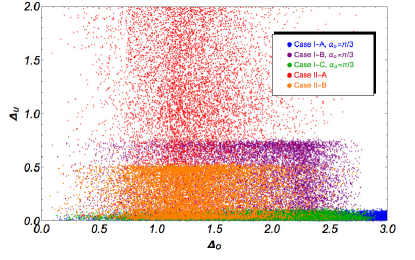
Figure 1: Plotting $\Delta_{O}$ versus $\Delta_{U}$ for the five cases indentified in Eq. (59) with $\alpha_{o}=\pi/3$.

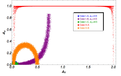
Figure 2: Plotting $\Delta_{O}$ versus $\Delta_{U}$ for the five cases indentified in Eq. (59) with $\alpha_{o}=\pi/3$.

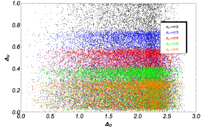
Figure 3: Plotting $\Delta_{O}$ versus $\Delta_{U}$ for the case I-B varying $\alpha_{o}=\pi/2$, $\pi/3$, $\pi/4$, $\pi/6$ and $\pi/9$.

Given the relevance of Scenario I-A, we shall now reproduce this scenario in the Standard Parametrization given in Eq. (1), where the TBM-scheme is obtained with

$$V^{SP}\,=\,O_{23}^{\pi/4}\cdot K_{{}_{D}}\cdot O_{13}\cdot O_{12}^{\phi_{o}}\,,\quad\sin\phi_{o}=\frac{1}{\sqrt{3}}\,,$$ (58)

with the angle of $O_{13}$ put to zero. For simplicity, we leave out the Majorana phases. In this parametrization, in order to have a value for $\left|V_{13}\right|\neq 0$, we have to switch on the angle $O_{13}$. However, for the unitary matrix in Eq. (58), one may check that even then, $\left|V_{23}\right|=\left|V_{33}\right|$, irrespective of the value of the angle of $O_{13}$. Thus, using this remaining parameter, one can not adjust the atmospheric mixing angle, unless, e.g. from the start, the angle of the $O_{23}$ is chosen to be different from $\pi/4$. One has to correct the atmospheric mixing angle, or from the beginning, or afterwards, with some additional extra contribution which modifies the TBM-limit. It is clear, in the Standard Parametrization, adjusting the TBM-limit for the atmospheric mixing angle is not possible using the remaining parameters. This is in clear contrast with our new parametrization and what we obtain for Scenario I-A, where the parameters available in the actual parametrization, in this case, via suitable choice for of the parameter $\varepsilon\,t_{23}$ in Eq. (58)), at the same time adjust the atmospheric mixing angle, generate a small value for $\left|V_{13}\right|$, and make possible large values for CP violation. Possibly, this may be useful for some model.

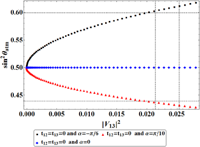
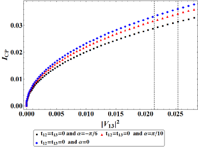
Figure 4: Plotting $\sin^{2}\theta_{atm}$ and the CP invariant $I_{cp}$ as a function of $|V_{13}^{2}|$ for scenario I-A.

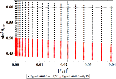
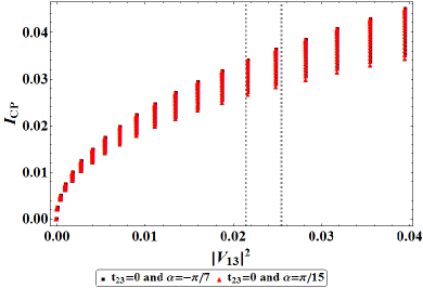
Figure 5: Plotting $\sin^{2}\theta_{atm}$ and the CP invariant $I_{cp}$ as a function of $|V_{13}^{2}|$ for scenario II-A.

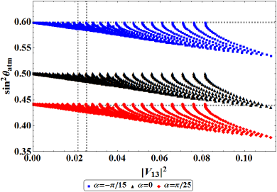
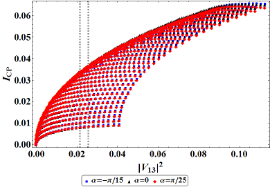
Figure 6: Plotting $\sin^{2}\theta_{atm}$ and the CP invariant $I_{cp}$ as a function of $|V_{13}^{2}|$ for scenario II-B.

V Numerical Simulation and Stability

For completeness, we give a numerical analysis of some of the scenarios described in the previous section. We choose a fixed scheme, the TBM scheme constructed with the 5 different scenarios. More precisely, we test

I-A $$:\qquad V_{o}=O_{23}^{\pi/4}O_{12}^{\phi_{o}}\,K_{\alpha_{o}}^{i}$$ (59)

I-B $$:\qquad V_{o}=O_{23}^{\pi/4}\,K_{\alpha_{o}}^{i}O_{12}^{\phi_{o}}$$

I-C $$:\qquad V_{o}=O_{23}^{\pi/4}\,O_{12}^{\phi_{1}}K_{\alpha_{o}}^{i}O_{12}^{\phi_{2}}$$

II-A $$:\qquad V_{o}=O_{23}^{\pi/4}O_{12}^{\phi_{o}}\,$$

II-B $$:\qquad V_{o}=O_{23}^{\theta_{o}}\,K_{\alpha_{o}}^{i}O_{23}^{\pi/4}O_{12}^{\phi_{o}}$$

where $\sin\phi_{o}=\sin\theta_{o}=\frac{1}{\sqrt{3}}$, $\sin\phi_{1}=\frac{1}{2}$, $\sin\phi_{2}=\frac{1}{\sqrt{6}}$. We define the $U_{o}$ as the matrix on the left of, together with the $K_{\alpha_{o}}^{i}$. In the II-A case, this is the identity matrix. We define also the $O_{o}$ as the matrix on the right of the $K_{\alpha_{o}}^{i}$. In the II-A case, this is the whole matrix $V_{o}$. For case II-B, $\alpha_{o}=0$ as pointed out in the previous section. For the other cases, we assume for $\alpha_{o}$, diverse fixed values.

We illustrate in Figs. 4-6 the correlations among the observables for the scenarios I-A, II-A and II-B. The figures plot for each scenario $\sin^{2}\theta_{atm}$ and $I_{CP}$ as a function of $|V_{13}|^{2}$ and $I_{CP}$ as a function of $|V_{13}|^{2}$, for particular values of the parameters left unconstrained in the definition of each scenario according to Table 1. Scenarios I-B and I-C are omitted since they have similar behavior as scenario I-A for these observables. A numerical analysis of Scenario I-A, was also done in Ref. Branco et al. (2015). We can conclude from Figs. 4-6 that a large CP invariant $I_{CP}$ can be obtained in agreement with the allowed experimental range of the observed parameters.

Next, we test how the lepton mixing matrix changes and the stability of our scenarios, by adding a small random perturbation to a predefined exact degenerate limit. To do this, we construct a neutrino mass matrix $M$, composed of an exact degenerate part in the form of a symmetric unitary matrix $S_{o}$ related to one of the TBM scenario schemes in Eq. (59), and a part composed of a small random perturbation $Q^{\varepsilon}$. Thus, the full quasi-degenerate neutrino mass matrix is as in Eq. (27):

$$M\,=\,\mu\,\left(S_{o}+Q^{\varepsilon}\right)\,,$$ (60)

where $S_{o}=U_{o}^{\ast}\,U_{o}^{\dagger}$, with the $U_{o}$’s of the different cases, and $Q^{\varepsilon}$ is some small complex symmetric random perturbation:

$$Q^{\varepsilon}\equiv\varepsilon^{2}\ Q\,,\quad\varepsilon^{2}=\frac{\left(\Delta m_{31}^{2}\right)^{\exp}}{2\mu^{2}}\,,$$

with $Q$ random perturbations of $O(1)$ generated by our program. We test the stability of lepton mixing of the different scenarios. We do not worry about the exact mass differences, with two (reasonable) exceptions: we take for $\varepsilon^{2}\$a fixed value. Inserting $\left(\Delta m_{31}^{2}\right)^{\exp}=2.5\times 10^{-3}\,\text{eV}^{2}$ together with a common neutrino mass $\mu\gtrsim 0.15\,\text{eV,}$ we obtain $\varepsilon^{2}\lesssim 0.05$; $\varepsilon$ is of the order of the Cabibbo angle. These values make sure that we are in a mass range where the computed output $\Delta m_{31}^{2}=O(1)\times 10^{-3}\,\text{eV}^{2}$. We discard cases generated by the perturbation where $\left|\Delta m_{31}^{2}\right|<\left|\Delta m_{21}^{2}\right|$. Further, we do not impose any other restrictions on the random perturbation $Q$ other than $Re(Q_{ij})$ and $Im(Q_{ij})$ to be real numbers between -1 and 1. However, we have checked that further restrictions on the masses do not change significantly any of the plots.

From the different mixing scenarios and the random $Q$’s in $M$, we compute the full lepton mixing $V$, i.e. the corresponding diagonalizing matrix matrix of $M$, such that $V^{\intercal}M\ V=D$ is real and positive. Following the proof in Section II, we decompose the full lepton mixing $V$ in the new parametrization, obtained as in Eq. (19). We then compare the new $U\equiv O_{23}\,O_{12}\,K_{\alpha}^{i}$ resulting from the perturbation, with the original $U_{o}$ (i.e., without the perturbation) of one of the cases in Eq. (59), and evaluate a quantity $\Delta_{U}$ giving a reasonable measure of how much $U$ and $U_{o}$ differ:

$$\Delta_{U}\,=\,\frac{1}{2}\sum\left|\,\left|U_{ij}\right|-\left|(U_{o})_{ij}\right|\,\right|\,.$$ (61)

Notice that this definition does not ”see” the phase factors of the $K_{\alpha}^{i}$ of $U$, or of the $U_{o}$. For this, we evaluate the changing on the phases $\alpha$ by defining the quantity

$$\Delta_{\alpha}\,=\,\left|\,\left|\sin\alpha\right|-\left|\sin\alpha_{o}\right|\,\right|\,,$$ (62)

that compares the phase $\alpha$ of the $K_{\alpha}^{i}$ of $U$, with the phase $\alpha_{o}$ of the $K_{\alpha_{o}}^{i}$ of $U_{o}$ and discarding differences of $\pi$. The $II-A$ case, has no $\alpha_{o}$ phases. We have also estimated how much $O$ in Eq. (19) differs from our original $O_{o}$ in Eq. (59), with

$$\Delta_{O}\,=\,\frac{1}{2}\sum\left|\,\left|O_{ij}\right|-\left|(O_{o})_{ij}\right|\,\right|\,,$$ (63)

where again we discard any sign difference. The $1/2$ in front of $\Delta_{O}$ (and $\Delta_{U}$) is a suitable normalization factor, chosen such that, e.g. in a case where the original $O_{o}=\mathbbm{1}$ and the new $O$ is such that $O=O_{12}$ (or any other elementary rotation) with an angle $\sin\theta_{12}=0.2$, then also $\Delta_{O}\approx 0.2$, of the same order of the Cabibbo angle.

In Fig. 1 and  2 we plot $\Delta_{U}$ as a function of $\Delta_{O}$ and $\Delta_{\alpha}$ as a function of $\Delta_{U}$, respectively, for the five scenarios. From Fig. 1 and  2 we find that the $\Delta_{U}$ and $\Delta_{\alpha}$ of Scenarios I-A and I-C hardly suffer any change with the perturbations. In Fig. 3, we show the variation of $\Delta_{O}$ as a function of $\Delta_{U}$ for different values of $\alpha_{o}=\pi/2$, $\pi/3$, $\pi/4$, $\pi/6$ and $\pi/9$ for Case I-B. Clearly, small $\alpha$ leads to more stability. Case I-A is not shown, since there is no apparent change of these quantities by varying $\alpha$.

Cases I-A, I-C and I-B with small $\alpha$ are the most stable with regard to $\Delta_{U}$ and $\Delta_{\alpha}$. As mentioned previously, Case I-C is somewhat artificial as it requires a certain conspiracy between two angles $\phi_{1}$ and $\phi_{2}$ angles to be near the TBM limit. Therefore, we focus on Case I-A. As shown in the previous section, generically, Scenario I-A has also the largest Majorana phases.

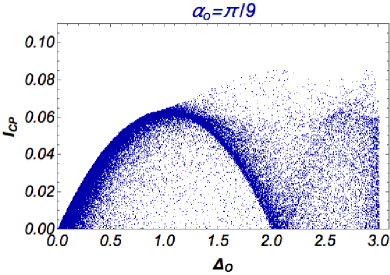
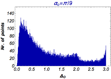
Figure 7: Plotting the CP invariant $I_{CP}$ as a function of $\Delta_{O}$ considering restricted perturbations for $Q$. The right-handed plot is an histogram showing the distribution of the values of $\Delta_{O}$ obtained from $50000$ uniformly distributed sets of input values for $Q$, restricted as indicated in Eq. (64).

With regard to the stability and variation of $\Delta_{O}$, we see that, in general, the perturbations generate large $\Delta_{O}$ contributions for all cases and in particular for Scenario I-A. It seems that this can only be improved if one imposes restrictions on the allowed perturbations forcing smaller $\Delta_{O}$’s. Maybe some kind of symmetry could accomplish this. In Fig. 7 we give an example, where the perturbations $Q$ are restricted: certain elements are taken to be zero, while the imaginary part and the diagonal real part are taken to be $0.1$ smaller than the others:

$$Q\,=\,\begin{pmatrix}0&0&0\\ 0&\frac{x_{22}}{10}&x_{23}\\ 0&x_{23}&\frac{x_{33}}{10}\end{pmatrix}+\frac{i}{10}\begin{pmatrix}0&0&0\\ 0&y_{22}&y_{23}\\ 0&y_{23}&y_{33}\end{pmatrix}$$ (64)

where the $x$’s, $y$’s are random real numbers varying between -1 and 1. For the initial phase $\alpha_{o}$, we take $\alpha_{o}=\pi/9$. We see that most of the deviations $\Delta_{O}$ (from the original $O_{o}=\mathbbm{1}$), are now around $0.2$ of the order of the Cabibbo angle, and this does not affect having large values for $I_{CP}$.

VI Conclusions

We have studied some aspects of leptonic CP violation from a new perspective. We have identified several limit scenario-cases, with mixing angles in agreement with experiment and leading to large CP violation. We proposed a new parametrization for leptonic mixing of the form $V=O_{23}\,O_{12}\,K_{\alpha}^{i}\cdot O$ to accomplish this.

If neutrinos are quasi-degenerate and Majorana, this parametrization is very useful. It may reflect some specific nature of neutrinos, suggesting that there is some major intrinsic Majorana character of neutrino mixing and CP violation, present in the left part of the parametrization, while the right part in the form of a real-orthogonal matrix $O$ with the 3 angles, reflects the fact that there are 3 neutrino families with small mass differences and results in small mixing. Thus, the intrinsic Majorana character of neutrinos may be large with a large contribution to neutrino mixing (from some yet unknown source), while the extra mixing $O$ of the families is comparable to the quark sector and may be small, of the order of the Cabibbo angle.

The new parametrization permits a new view of large leptonic CP violation. It shows interesting aspects that were less clear for the standard parametrization. We identified several limit scenario-cases and shown results for mixing and CP violation. A certain scenario (I-A) was found to be the most appealing. It only needs 2 extra parameters to fit the experimental results on lepton mixing and provides large Dirac-CP violation and large values for the Majorana-CP violating phases. We point out that the results for this scenario derives explicitly from the form of the new parametrization.

In addition and for quasi-degenerate Majorana neutrinos, the stability of the different scenarios was tested using random perturbations. We concluded that the left part of the parametrization behaves quite differently for the diverse scenarios. Scenario I-A was very stable in this respect. With respect to the right part of the parametrization, i.e., the real-orthogonal matrix $O$, the perturbations generate large contributions for all cases. This unstable part of the mixing (due to the random perturbations) can only be improved, if one imposes restrictions on the allowed perturbations. We have shown how to accomplish this.

References

- Branco et al. (2012a) G. Branco, R. G. Felipe, and F. Joaquim, Rev. Mod. Phys. 84, 515 (2012a), arXiv:1111.5332 [hep-ph] .
- King et al. (2014) S. F. King, A. Merle, S. Morisi, Y. Shimizu, and M. Tanimoto, New J. Phys. 16, 045018 (2014), arXiv:1402.4271 [hep-ph] .
- Shimizu and Tanimoto (2015) Y. Shimizu and M. Tanimoto, Mod. Phys. Lett. A30, 1550002 (2015), arXiv:1405.1521 [hep-ph] .
- Wang et al. (2013) B. Wang, J. Tang, and X.-Q. Li, Phys. Rev. D 88, 073003 (2013), arXiv:1303.1592 [hep-ph] .
- King and Luhn (2013) S. F. King and C. Luhn, Rept. Prog. Phys. 76, 056201 (2013), arXiv:1301.1340 [hep-ph] .
- Boucenna et al. (2012) S. Boucenna, S. Morisi, M. Tortola, and J. Valle, Phys. Rev. D 86, 051301 (2012), arXiv:1206.2555 [hep-ph] .
- Ferreira et al. (2012) P. Ferreira, W. Grimus, L. Lavoura, and P. Ludl, J. High Energy Phys. 1209, 128 (2012), arXiv:1206.7072 [hep-ph] .
- Branco et al. (2012b) G. Branco, R. González Felipe, F. Joaquim, and H. Serôdio, Phys. Rev. D 86, 076008 (2012b), arXiv:1203.2646 [hep-ph] .
- Hernandez and Smirnov (2013a) D. Hernandez and A. Y. Smirnov, Phys. Rev. D 87, 053005 (2013a), arXiv:1212.2149 [hep-ph] .
- Eby and Frampton (2012) D. A. Eby and P. H. Frampton, Phys. Rev. D 86, 117304 (2012), arXiv:1112.2675 [hep-ph] .
- Ge et al. (2012) S.-F. Ge, D. A. Dicus, and W. W. Repko, Phys. Rev. Lett. 108, 041801 (2012), arXiv:1108.0964 [hep-ph] .
- Toorop et al. (2011) R. d. A. Toorop, F. Feruglio, and C. Hagedorn, Phys. Lett. B 703, 447 (2011), arXiv:1107.3486 [hep-ph] .
- Zhou (2011) S. Zhou, Phys. Lett. B 704, 291 (2011), arXiv:1106.4808 [hep-ph] .
- Altarelli and Feruglio (2010) G. Altarelli and F. Feruglio, Rev. Mod. Phys. 82, 2701 (2010), arXiv:1002.0211 [hep-ph] .
- Datta et al. (2005) A. Datta, L. Everett, and P. Ramond, Phys. Lett. B 620, 42 (2005), arXiv:hep-ph/0503222 [hep-ph] .
- Hernandez and Smirnov (2013b) D. Hernandez and A. Y. Smirnov, Phys. Rev. D 88, 093007 (2013b), arXiv:1304.7738 [hep-ph] .
- Hall et al. (2000) L. J. Hall, H. Murayama, and N. Weiner, Phys. Rev. Lett. 84, 2572 (2000), arXiv:hep-ph/9911341 [hep-ph] .
- Haba and Murayama (2001) N. Haba and H. Murayama, Phys. Rev. D 63, 053010 (2001), arXiv:hep-ph/0009174 [hep-ph] .
- de Gouvea and Murayama (2003) A. de Gouvea and H. Murayama, Phys. Lett. B 573, 94 (2003), arXiv:hep-ph/0301050 [hep-ph] .
- Altarelli et al. (2012) G. Altarelli, F. Feruglio, I. Masina, and L. Merlo, J. High Energy Phys. 1211, 139 (2012), arXiv:1207.0587 [hep-ph] .
- Pontecorvo (1957) B. Pontecorvo, Sov. Phys. JETP 6, 429 (1957).
- Maki et al. (1962) Z. Maki, M. Nakagawa, and S. Sakata, Prog. Theor. Phys. 28, 870 (1962).
- Pontecorvo (1968) B. Pontecorvo, Sov. Phys. JETP 26, 984 (1968).
- Harrison et al. (2002) P. Harrison, D. Perkins, and W. Scott, Phys. Lett. B 530, 167 (2002), arXiv:hep-ph/0202074 [hep-ph] .
- Branco et al. (1999a) G. Branco, M. Rebelo, and J. Silva-Marcos, Phys. Rev. Lett. 82, 683 (1999a), arXiv:hep-ph/9810328 [hep-ph] .
- Silva-Marcos (2002) J. Silva-Marcos, (2002), arXiv:hep-ph/0212089 [hep-ph] .
- Branco et al. (2015) G. Branco, M. Rebelo, J. Silva-Marcos, and D. Wegman, Phys. Rev. D 91, 013001 (2015), arXiv:1405.5120 [hep-ph] .
- Wolfenstein (1981) L. Wolfenstein, Phys. Lett. B 107, 77 (1981).
- Branco et al. (1999b) G. C. Branco, L. Lavoura, and J. P. Silva, Int. Ser. Monogr. Phys. 103, 1 (1999b).
- Forero et al. (2014) D. Forero, M. Tórtola, and J. Valle, Phys. Rev. D 90, 093006 (2014), arXiv:1405.7540 [hep-ph] .
- Kajiyama et al. (2007) Y. Kajiyama, M. Raidal, and A. Strumia, Phys. Rev. D 76, 117301 (2007), arXiv:0705.4559 [hep-ph] .
- Giunti (2003) C. Giunti, Nucl. Phys. Proc. Suppl. 117, 24 (2003), arXiv:hep-ph/0209103 [hep-ph] .
- Xing (2003) Z.-z. Xing, J. Phys. G 29, 2227 (2003), arXiv:hep-ph/0211465 [hep-ph] .