Meta learning of bounds on the Bayes classifier error

Abstract

Meta learning uses information from base learners (e.g. classifiers or estimators) as well as information about the learning problem to improve upon the performance of a single base learner. For example, the Bayes error rate of a given feature space, if known, can be used to aid in choosing a classifier, as well as in feature selection and model selection for the base classifiers and the meta classifier. Recent work in the field of $f$-divergence functional estimation has led to the development of simple and rapidly converging estimators that can be used to estimate various bounds on the Bayes error. We estimate multiple bounds on the Bayes error using an estimator that applies meta learning to slowly converging plug-in estimators to obtain the parametric convergence rate. We compare the estimated bounds empirically on simulated data and then estimate the tighter bounds on features extracted from an image patch analysis of sunspot continuum and magnetogram images.

Index Terms—  Bayes error, divergence estimation, meta learning, classification, sunspots

1 Introduction

Meta learning is a method of learning from learned knowledge that can be used to improve the performance of various learning tasks [1, 2]. In a typical example where the learning task is classification, meta learning is applied by first training multiple classifiers on the training data. Each classifier may use either all of the training data, or only a subset which may differ from other subsets in the feature space. A test set is then fed into these classifiers and the resulting output is then used as input to train an overall meta classifier such as a majority vote or weighted majority vote. Other variations on meta learning applied to classification exist [2, 3, 4].

Meta learning can incorporate information about the feature space that is independent of the classifiers such as the Bayes error rate (BER). Consider the problem of classifying a feature vector $x$ into one of two classes $C_{1}$ or $C_{2}$. Denote the a priori class probabilities as $q_{1}=\Pr(C_{1})>0$ and $q_{2}=\Pr(C_{2})=1-q_{1}>0$. The conditional densities of $x$ given that $x$ belongs to $C_{1}$ or $C_{2}$ are denoted by $f_{1}(x)$ and $f_{2}(x)$, respectively, and the Bayes classifier assigns $x$ to $C_{1}$ if and only if $q_{1}f_{1}(x)>q_{2}f_{2}(x)$. If $p(x)=q_{1}f_{1}(x)+q_{2}f_{2}(x)$, the average error rate of this classifier, known as the BER, is

$$P_{e}^{*} = \int\min\left(\Pr\left(C_{1}|x\right),\Pr\left(C_{2}|x\right)\right)p(x)dx$$ (1)

$$= \int\min\left(q_{1}f_{1}(x),q_{2}f_{2}(x)\right)dx.$$

The BER is the minimum classification error rate that can be achieved by any classifier on $x$’s feature space [5]. Because of this property, the BER can be used in a meta learning problem where the base classifiers are trained on different feature spaces by weighting the output of the base classifiers based on the Bayes error of the underlying feature space. If a given feature space results in a lower Bayes error than another feature space, then the output of the corresponding classifier would have a higher weight as it would presumably perform better than a classifier on the alternate feature space.

The BER can be used at other stages of meta learning such as in the selection of the base classifiers and model selection. This is because the BER provides a benchmark for classification on a given feature space. If a specific classifier applied to the feature space yields an estimated error rate that is significantly above the BER, then it is likely that a different classifier or parameters may result in a lower error rate. On the other hand, if the classifier’s estimated error rate is below the BER, then the classifier is likely to be overfitting the data and may not generalize well to new samples from the feature space. A different classifier or parameters may then be chosen. This technique can also be applied in the traditional supervised learning approach where a single classifier is used.

The BER can also be beneficial for feature selection in classification problems. The BER is monotonic in the number of features in the sense that increasing the number of features does not decrease the accuracy of the Bayes classifier. However, for many classifiers, including irrelevant features can decrease the prediction accuracy [6, 7]. Including a large number of features can also be computationally burdensome and create difficulties in storage and memory [8, 9]. Thus from a practical perspective, using only a subset of the features may result in better performance. If the BER is known for all subsets of features, then a logical method of feature selection would be to choose the smallest subset of features such that the BER of that subset is negligibly larger than the BER of the full feature space [10]. The eliminated features could be considered redundant or irrelevant since including them in the classification leads to a neglible improvement in accuracy.

Unfortunately, computing the BER requires perfect knowledge of the underlying data distributions, which is rarely available. Even for parametric models of the densities, Eq. 1 requires multi-dimensional integration and has no closed form solution for many models. Evaluating the BER in these cases involves computationally intensive numerical integration, especially for high dimensions. For these reasons, many feature selection algorithms have focused on other optimality criteria such as minimizing the prediction error of a specific classifier [7] or maximizing the statistical dependency between the feature subset and class assignments via some criterion such as mutual information or correlation [11]. However, selecting features by minimizing the classifier prediction error can be computationally intensive and only provides a solution for the specified classifier. Additionally, other methods based on maximizing statistical dependency can be too restrictive or otherwise problematic [12].

Given these problems, many bounds on the BER have been derived that are related to $f$-divergences [13, 14, 15, 16]. These bounds have been used in applications involving the BER including feature selection [14, 17, 18, 19, 20].

Accurate estimation of these bounds on the BER requires accurate estimation of an $f$-divergence functional, often in a nonparametric setting. Until recently, little has been known about the properties of nonparametric $f$-divergence estimators such as convergence rates and the asymptotic distribution. In Moon and Hero [21], it was shown that the bias of simple density plug-in estimators of $f$-divergence converges very slowly to zero when the dimension of the feature space is high, which limits their utility. Nguyen et al [22] proposed an $f$-divergence estimation method based on estimating the likelihood ratio of two densities that achieves the parametric mean squared error (MSE) convergence rate when the densities are sufficiently smooth. However, this method can be computationally intensive for large sample sizes and the asymptotic distribution of the estimator is currently unknown. Berisha et al [14] also proposed a consistent estimator of specific bounds on the BER based on the construction of a minimal spanning tree (MST) that does not require density estimation. However, the convergence rate of this estimator is unknown and it is restricted to specific BER bounds instead of $f$-divergences in general. Finally, other $f$-divergence estimators have been proposed that achieve the parametric rate when the densities are sufficiently smooth [23, 24, 25]. However, some of these estimators are restricted to certain subsets of $f$-divergences, and they require an optimal kernel which can be difficult to implement and compute.

Many of these problems can be countered effectively by using meta learning. While meta learning was described above in the classification setting, it can also be applied to estimation to improve the convergence rates. This is typically done by taking a weighted sum of base estimators that individually converge slowly. Then by an appropriate choice of weights, the weighted ensemble estimator converges rapidly to the true value. For example, Sricharan et al [26] derived a nonparametric estimator of generalized entropy functionals that converges at the parametric rate by using simple plug-in density estimators as the base estimators. More recently, similar theory was applied by Moon and Hero [21, 27] to obtain a nonparametric $f$-divergence functional estimator based on a weighted ensemble of $k$-nearest neighbor (nn) estimators. This estimator enjoys the advantages of being simple to implement and achieving the parametric convergence rate when the densities are sufficiently smooth.

In this paper, we focus on estimating multiple bounds on the Bayes error derived from $f$-divergence functionals in a nonparametric setting using the weighted $k$-nn estimator from [21, 27]. We first estimate the bounds on simulated data where the true BER is computable. This gives a guide for the empirical utility of each bound. We then apply this to real data by estimating the bounds on the BER for the classification of sunspot images using the features derived in [28]. This gives a measure of the utility of the derived feature space in this supervised setting. We also compare the results to those obtained usinge the MST estimator [14]. The paper is outlined as follows. Section 2 describes the weighted $k$-nn estimator of $f$-divergence functionals while Section 3 provides the bounds on the Bayes error and their relation to $f$-divergences. In Section 4, the simulated results are presented. Section 5 describes the sunspot data and presents the estimated bounds on the BER. Section 6 concludes.

2 Meta Learning of $f$-Divergence Functionals

If $f_{1}$ and $f_{2}$ are $d$-dimensional probability densities with common support, then the $f$-divergence between $f_{1}$ and $f_{2}$ has the following form [29]:

$$D_{\phi}(f_{1},f_{2})=\int\phi\left(\frac{f_{1}(x)}{f_{2}(x)}\right)f_{2}(x)dx.$$ (2)

For $D_{\phi}$ to be considered a true divergence, the function $\phi$ must be convex and $\phi(1)=0$. This ensures that $D_{\phi}$ is nonnegative and that $D_{\phi}(f_{1},f_{2})=0$ if and only if $f_{1}=f_{2}$ which is the definition of divergence. As for general divergences, $f$-divergences are not required to be symmetric or satisfy the triangle inequality.

In this work, we are concerned with a broader class of functions that we call $f$-divergence functionals. This class consists of functions of the form in Eq. 2 except that we do not require $\phi$ to be convex or that $\phi(1)=0$. Working with $f$-divergence functionals instead of only $f$-divergences provides greater flexibility in bounding the BER.

Assume that the densities $f_{1}$ and $f_{2}$ have a common bounded support set $\mathcal{S}$; $f_{1}$ and $f_{2}$ are strictly lower bounded; and $f_{1}$, $f_{2}$, and $\phi$ are smooth. Assume that $T=N+M$ i.i.d. realizations $\mathcal{X}_{T}=\left\{\mathbf{X}_{1},\dots,\mathbf{X}_{N},\mathbf{X}_{N+1},\dots,\mathbf{X}_{N+M}\right\}$ are available from the density $f_{2}$ and $M$ i.i.d. realizations $\mathcal{Y}_{M}=\left\{\mathbf{Y}_{1},\dots,\mathbf{Y}_{M}\right\}$ are available from the density $f_{1}$, where $M$ is proportional to $T$. Under these assumptions, there exists a nonparametric estimator of $D_{\phi}$ that achieves the parametric MSE rate of $O\left(\frac{1}{T}\right)$. This estimator first calculates an ensemble of $k$-nn density estimators of the densities $f_{1}$ and $f_{2}$ at the points $\left\{\mathbf{X}_{1},\dots,\mathbf{X}_{N}\right\}$ using different values of $k$. Then for each $k$, a base plug-in estimator of $D_{\phi}$ is calculated by taking the empirical average of the $\phi$ evaluated at the likelihood ratio of the estimated densities. From [21], the bias and variance of these base estimators is known. Then using the theory of optimally weighted ensemble estimation [26], an estimator with low bias can be obtained by taking a weighted sum of the base estimators using the appropriate weights. Details are given in the following.

Let $k\leq M$ and let $\mathbf{\rho}_{2,k}(i)$ be the distance of the $k$th nearest neighbor of $\mathbf{X}_{i}$ in $\left\{\mathbf{X}_{M+1},\dots,\mathbf{X}_{N}\right\}$. Similarly, define $\mathbf{\rho}_{1,k}(i)$ be the distance of the $k$th nearest neighbor of $\mathbf{X}_{i}$ in $\left\{\mathbf{Y}_{1},\dots,\mathbf{Y}_{M}\right\}$. Then the $k$-nn density estimates at the point $\mathbf{X}_{i}$ are [30]

$$\hat{\mathbf{f}}_{j,k}(\mathbf{X}_{i})=\frac{k}{M\bar{c}\mathbf{\rho}_{j,k}^{d}(i)},$$

where $\bar{c}$ is the volume of a $d$-dimensional unit ball. The functional $D_{\phi}$ is then approximated as

$$\hat{\mathbf{D}}_{\phi,k}=\frac{1}{N}\sum_{i=1}^{N}\phi\left(\frac{\hat{\mathbf{f}}_{1,k}(\mathbf{X}_{i})}{\hat{\mathbf{f}}_{2,k}(\mathbf{X}_{i})}\right).$$

Now choose an ensemble of positive real numbers $\bar{\ell}=\left\{\ell_{1},\dots,\ell_{L}\right\}$ where $L>d-1$ and let $k(\ell)=\ell\sqrt{M}$. It was shown in [21] that the bias and variance of $\hat{\mathbf{D}}_{\phi,k(\ell)}$ are

$$\text{Bias}\left(\hat{\mathbf{D}}_{\phi,k(\ell)}\right) = \sum_{j=1}^{d}O\left(\left(\frac{\ell}{\sqrt{M}}\right)^{\frac{j}{d}}\right)+O\left(\frac{1}{\sqrt{M}}\right),$$

$$\text{Var}\left(\hat{\mathbf{D}}_{\phi,k(\ell)}\right) = O\left(\frac{1}{N}+\frac{1}{M}\right).$$

Let $w$ be a vector of weights with length $L$ and define $\hat{\mathbf{D}}_{\phi,w}:=\sum_{\ell\in\bar{\ell}}w(\ell)\hat{\mathbf{D}}_{\phi,k(\ell)}$. From the theory of optimally weighted ensemble estimation [26], there exists a weight vector $w_{0}$ such that the MSE of $\hat{\mathbf{D}}_{\phi,w_{0}}$ is $O\left(\frac{1}{T}\right)$. The weight vector $w_{0}$ achieves this by essentially zeroing out the lower order bias terms at the expense of a slight increase in the variance. $w_{0}$ can be found via an offline convex optimization problem that only depends on the sample size $T$ and the basis functions $\ell^{\frac{j}{d}}$. See [21, 26, 27] for more details.

3 Bounds on the Bayes Error Rate

Multiple upper and lower bounds on the BER related to $f$-divergences exist. A classical bound is the Chernoff bound [13]. It is derived from the fact that for $a,\,b>0$, $\min(a,b)\leq a^{\alpha}b^{1-\alpha}$ $\forall\alpha\in(0,1)$. Replacing the minimum function in Eq. 1 with this bound gives

$$P_{e}^{*}\leq q_{1}^{\alpha}q_{2}^{1-\alpha}c_{\alpha}(f_{1},f_{2}),$$ (3)

where $c_{\alpha}(f_{1},f_{2})=\int f_{1}^{\alpha}(x)f_{2}^{1-\alpha}(x)dx$ is the Chernoff $\alpha$-coefficient. The Chernoff coefficient is found by minimizing the right hand side of Eq. 3 with respect to $\alpha$:

$$c^{*}(f_{1},f_{2})=\min_{\alpha\in(0,1)}\int f_{1}^{\alpha}(x)f_{2}^{1-\alpha}(x)dx.$$ (4)

Combining this with Eq. 3 gives an upper bound on the BER.

In general, the Chernoff bound is not very tight. A tighter bound was presented in [14]. Consider the following quantity:

$$\tilde{D}_{q_{1}}(f_{1},f_{2}) = 1-4q_{1}q_{2}\int\frac{f_{1}(x)f_{2}(x)}{q_{1}f_{1}(x)+q_{2}f_{2}(x)}dx$$ (5)

$$= \int\frac{\left(q_{1}f_{1}(x)-q_{2}f_{2}(x)\right)^{2}}{q_{1}f_{1}(x)+q_{2}f_{2}(x)}dx.$$ (6)

It was shown in [14] that the BER $P_{e}^{*}$ is bounded above and below as follows:

$$\frac{1}{2}-\frac{1}{2}\sqrt{\tilde{D}_{q_{1}}(f_{1},f_{2})}\leq P_{e}^{*}\leq\frac{1}{2}-\frac{1}{2}\tilde{D}_{q_{1}}(f_{1},f_{2}).$$

Arbitrarily tight upper and lower bounds to the BER were given in [15]. We consider only the lower bound here. Define

$$g_{\alpha}(f_{1},f_{2})=\ln\left(\frac{1+e^{-\alpha}}{\exp\left(\frac{-\alpha q_{1}f_{1}(x)}{p(x)}\right)+\exp\left(\frac{-\alpha q_{2}f_{2}(x)}{p(x)}\right)}\right),$$

where $p(x)=q_{1}f_{1}(x)+q_{2}f_{2}(x)$ as before and $\alpha>0$. Then the BER is bounded below as

$$P_{e}^{*}\geq\frac{1}{\alpha}\int g_{\alpha}(f_{1},f_{2})p(x)dx=:G_{\alpha}(f_{1},f_{2}).$$ (7)

The functionals in Eqs. 3 and 5-7 all contain the form in Eq. 2. To see this, note that for the Chernoff $\alpha$ coefficient, $\phi(t)=t^{\alpha}$. For the $\tilde{D}_{q_{1}}$ based bounds, the functions are more complicated with $\phi(t)=\frac{4q_{1}q_{2}t}{q_{2}+q_{1}t}$ and $\phi(t)=\frac{\left(q_{1}t-q_{2}\right)^{2}}{q_{1}t+q_{2}}$ for Eqs. 5 and 6, respectively. The functions are even more complex for Eq. 7. However, if $t=\frac{f_{1}(x)}{f_{2}(x)}$, then

$$\exp\left(\frac{-\alpha q_{1}f_{1}(x)}{p(x)}\right) = \exp\left(\frac{-\alpha q_{1}}{q_{1}+q_{2}t^{-1}}\right),$$

$$\exp\left(\frac{-\alpha q_{2}f_{2}(x)}{p(x)}\right) = \exp\left(\frac{-\alpha q_{2}}{q_{2}+q_{1}t}\right).$$

Substituting these expressions into $G_{\alpha}(f_{1},f_{2})$ gives the required form. Thus we can use the optimally weighted ensemble divergence estimator from Section 2 to estimate all of these bounds on the Bayes error. To estimate $c^{*}(f_{1},f_{2})$, we estimate $c_{\alpha}(f_{1},f_{2})$ for multiple values of $\alpha$ (e.g. $0.01,\,0.02,\dots,0.99$) and choose the minimum.

4 Simulations

In addition to the weighted $k$-nn estimator, we use an alternate estimator for $\tilde{D}_{q_{1}}$ based on an extension of the Friedman-Rafsky (FR) multivariate two sample test statistic for comparison [31]. This estimator is derived from the MST of the combined data set $\mathcal{X}_{T}\cup\mathcal{Y}_{M}$ and does not require direct estimation of the densities $f_{1}$ and $f_{2}$ [14, 32]. However, the convergence rate and asymptotic distribution of this estimator are currently unknown.

Fig. 1: Estimated bounds on the Bayes error rate for two unit variance Gaussians with dimension $d=5$, varying sample sizes ($T=5000,\,50$), and varying means over 200 trials. Error bars correspond to a single standard deviation. The $\tilde{D}_{q_{1}}$ based lower bounds are close to the actual Bayes error for both the large and small sample regimes but are much more variant with a smaller sample size. The arbitrarily tight lower bound ($G_{\alpha}$ with $\alpha=500$) is very close to the Bayes error when $T=5000$ and when the Bayes error is low.

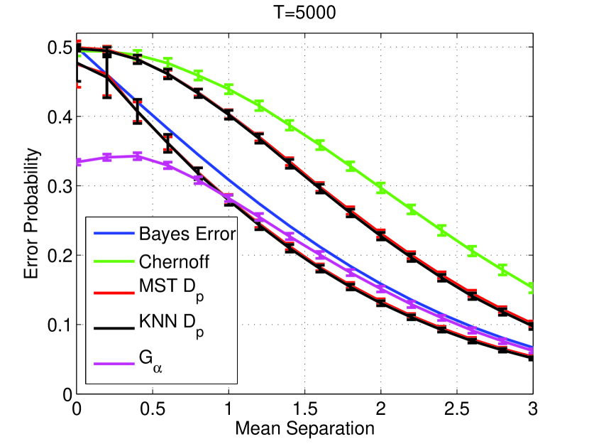
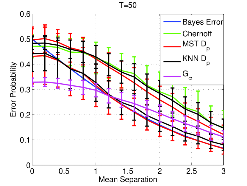
To compare the estimation performance of the various bounds on the BER, we consider 200 trials of two samples from two Gaussian distributions with unit variance and varying mean. In practice, we use a leave one out approach for the weighted $k$-nn estimator and so the number of samples from both distributions is equal to $T$. In the first experiment, we fix the dimension $d=5$ and vary the number of samples from each distribution. Figure 1 shows the cases where $T=5000$ and $50$. We choose $\alpha=500$ for $G_{\alpha}$. In the large sample regime, the bounds vary smoothly as the separation between the means of the distributions increases. The two methods for estimating $\tilde{D}_{q_{1}}$ have nearly identical results when Eq. 5 is used for the weighted $k$-nn method. If Eq. 6 is used, then the estimated bounds (not shown) are inaccurate. This underscores the importance of using an appropriate representation of the function $\phi$ when using plug-in based estimation methods as numerical errors may lead to varying results.

In the low sample regime, the estimates have much higher variance and are more biased as the lower bounds often cross the Bayes error. However, the $\tilde{D}_{q_{1}}$ based lower bounds are still fairly close to the true BER and are thus valuable for assessing the potential performance of a given feature space. Increasing the sample size to as little as 150 greatly improves the performance (not shown).

Fig. 2: Estimated bounds on the Bayes error rate for two unit variance Gaussians with varying dimension ($d=1,\,10$) and a fixed sample size of $T=1000$ over 200 trials. The estimated $\tilde{D}_{q_{1}}$ based bounds are more biased and variant when the dimension is higher.

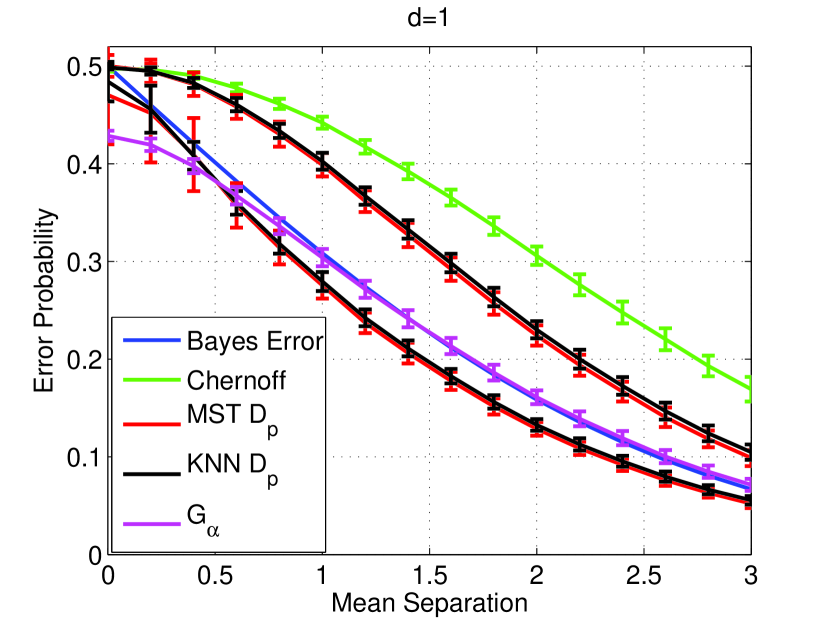
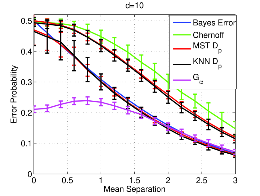
In the second experiment, we fixed the number of samples at $T=1000$ and varied the dimension. The results for $d=1$ and $10$ are given in Fig. 2. In the higher dimension, the $\tilde{D}_{q_{1}}$ lower bounds are closer to the BER which results in these estimates crossing over the BER more often. The variance in all of the estimates is also higher when $d=10$.

Several trends are apparent in both Figs. 1 and 2. One is that the variance of the $\tilde{D}_{q_{1}}$ lower bounds decreases as the BER decreases. In general, the MST-based estimator is more variant than the $k$-nn estimator except when the dimension or number of samples is high (e.g. $d=10$ or $T=5000$). This is not a substantial problem as an accurate estimate of the BER is less useful at higher values. This is because if the BER is around 0.4, then the feature space being considered does not improve the classification much beyond random guessing. Thus time and energy may be better spent on finding a new feature space for the problem instead of attempting to achieve the BER on the given feature space.

Another observation is that for $d>1$, the $G_{\alpha}$ based lower bound is not tight for higher BER when using $\alpha=500$. Increasing $\alpha$ does not substantially improve the tightness at these values due to numerical precision errors. However, it may be possible to manipulate the expression for $g_{\alpha}$ so that this is not an issue.

Overall, these results suggest that estimating the $\tilde{D}_{q_{1}}$ lower bound provides a value that is fairly close to the true BER. The weighted $k$-nn estimator appears to be less variant than the MST based estimator except when the dimension or number of samples is sufficiently high. Thus we recommend using the $\tilde{D}_{q_{1}}$ bounds to estimate the location of the BER. If this gives a range for the BER that is low (approximately less than 0.2) and there are enough samples, then $G_{\alpha}$ may be estimated for a more precise estimate of the BER. Similar results are obtained for truncated Gaussians.

5 Bounding the Bayes Error of Sunspot Images

We estimate bounds on the BER of a sunspot image classification problem. Sunspots (SS) are dark areas seen in white light images of the Sun. They correspond to regions of locally enhanced magnetic field, as can be seen on magnetogram. SS groups are commonly classified using the Mount Wilson classification scheme, which categorizes them by eye based on their morphological features in continuum (white light intensity) and magnetogram (magnetic field value) images. Several studies have shown that major solar eruptive events are strongly correlated with complex SS groups (designated as $\beta\gamma$ or $\beta\gamma\delta$ groups) and less so with simple SSs ($\alpha$ or $\beta$ groups) [33, 34].

Recent work has focused on clustering SSs using an image patch analysis of continuum and magnetogram images and by applying dictionary learning on the collection of patches [28, 35]. Two main approaches were used in [28]. In the first approach, a dictionary is learned for each SS image pair. The pairwise difference between these dictionaries is calculated by comparing the subspaces spanned by the dictionaries using the Grassmannian projection metric. These pairwise distances are then fed into a clustering algorithm. For the second approach, a single dictionary is learned from the combined collection of image patches from all SS image pairs. The dictionary coefficients corresponding to a single SS image pair are treated as samples from a distribution. The pairwise distances between these collections of coefficient samples is calculated by estimating the Hellinger distance of the underlying distribution and these distances are then fed into a clustering algorithm.

The resulting clusterings from these two approaches were found to be correlated somewhat with the Mount Wilson classification scheme. In this work, we estimate the ability of the associated feature spaces of these two approaches to classify a SS as ‘complex’ or ‘simple’ by estimating bounds on the Bayes error. We do this by estimating both the lower and upper bounds formed from $\tilde{D}_{q_{1}}$ using both the weighted $k$-nn and MST estimators for the Grassmannian approach from the pairwise distances. Bootstrapping is used on the weighted $k$-nn estimators to calculate confidence intervals. For the Hellinger distances, we only use the MST estimator as the $k$-nn density estimator is not easily defined in the space of probability distributions.

We use the same image pairs as in [28] except we exclude the $\alpha$ groups. This is to keep the number of simple and complex image pairs roughly the same (192 and 182, respectively). As in [28], we consider two types of areas: the area within the sunspot and the area near the corresponding neutral line as determined from magnetogram images. The morphology of both of these areas are taken into account in the Mount Wilson classification. The two metrics, Grassmannian and Hellinger distance, are applied within these areas separately and a weighted average is taken of the two distances. For example, if $D_{G,n}$ is the distance matrix comparing the dictionaries learned from each SS’s neutral line using the Grassmannian metric, and if $D_{G,s}$ is the distance matrix comparing the dictionaries learned from within the sunspots, then define $D_{G}(r)=rD_{G,n}+(1-r)D_{G,s}$ with $0\leq r\leq 1$. The distance matrix $D_{G}(r)$ is then used to estimate the bounds on the Bayes error for a variety of weights. For comparison, we calculate the error rate of a support vector machine (SVM) classifier with a Gaussian kernel using 10-fold cross validation to select the parameters.

Two dictionary learning methods are used: the singular value decomposition (SVD) and nonnegative matrix factorization (NMF). Figure 3 shows the estimated bounds when using SVD. Several patterns are apparent in the results. Both the estimated bounds and the SVM error rate generally increase as the weight $r$ increases when the Grassmannian metric on individual dictionaries is used. This indicates that the dictionaries extracted from within the sunspots are more relevant to this classification problem than the dictionaries from the neutral line. The opposite occurs when the Hellinger distance is used on the dictionary coefficients. In this case, the estimated bounds and SVM error rate are generally lower when the weight $r$ favors the neutral line data. Strong spatial gradients in the magnetogram along the neutral line are often associated with complex SSs. Since the learned dictionaries contain patches with magnetogram gradients (see Figs. 4 and 5 in Moon et al [28]), the distributions of the corresponding coefficients within the neutral line may be useful for distinguishing between complex and simple ARs and thus lead to the decreased bounds on the BER and improved classification.

Fig. 3: $\tilde{D}_{q_{1}}$-based upper (plain line) and lower (dashed line) bounds on the Bayes error when classifying sunspot groups as simple or complex for a variety of weights compared to the error from an SVM classifier using SVD dictionaries. A weight of $r=0$ corresponds to using only the data from within the sunspots while $r=1$ corresponds to using only the neutral line data. Confidence intervals on the weighted $k$-nn estimators are calculated via bootstrapping. The area around the neutral line and sunspots give better results when using the Hellinger and Grassmannian metrics, respectively.

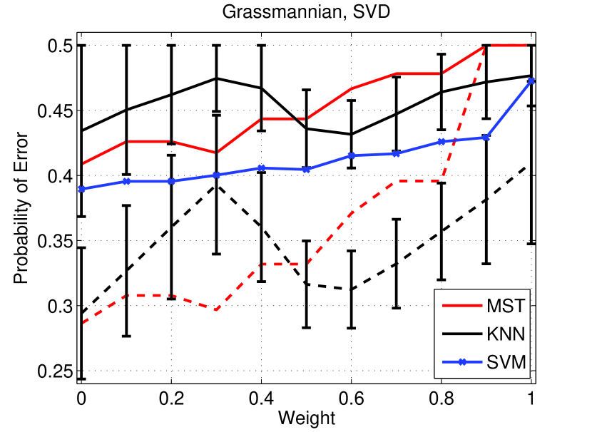
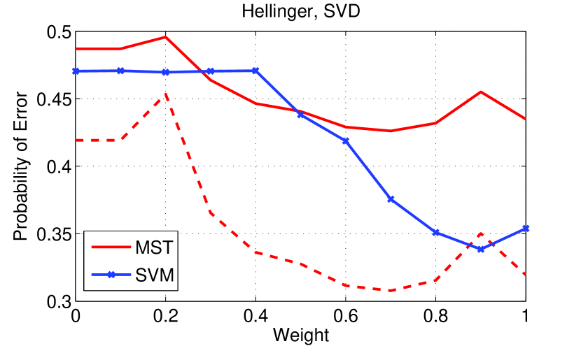
The NMF results are not shown, but similar trends are observed. For both the Grassmannian and Hellinger metrics, the estimated bounds and the SVM error rate generally decrease as the weight increases, suggesting that the neutral line is better suited for this classification problem than the data from within the sunspots when using NMF dictionaries. However, the estimated bounds, confidence intervals, and error rates are generally still high (>0.25).

In general, these results indicate that if the goal is to accurately classify SSs into complex or simple SSs based on the Mount Wilson definition, then additional or different features are required. The dictionary features may still be relevant for other learning tasks such as predicting and detecting solar eruptive events.

6 Conclusion

Applying meta learning or ensemble methods to the problem of estimating $f$-divergence functionals results in more accurate estimates. This ensemble estimator is useful for estimating multiple bounds on the Bayes error rate. By simulation, we found that the $\tilde{D}_{q_{1}}$ bounds are more accurate than the Chernoff bound and the $G_{\alpha}$ bound in the sense that they are tighter for all values of the BER. The $G_{\alpha}$ bound, however, is closer to the BER when it is small and when the dimension is low. The MST and weighted $k$-nn estimators had similar performance, suggesting that the MST based method may converge rapidly to the true value in at least some circumstances.

From the BER bounds of the sunspot data, we found that learned SVD dictionaries from the neutral line are unlikely to be helpful in classifying SSs (as either a simple SS or complex SS) based on the Mount Wilson definition. However, including the dictionary coefficients from the neutral line does seem to result in lower bounds on the BER and better classification performance than when just using the dictionary coefficients from within the sunspots. Overall, additional features are likely necessary to achieve accurate classification of sunspots into these categories.

References

- [1] P. K. Chan and S. J. Stolfo, “Meta-learning for multistrategy and parallel learning,” in Proc. 2nd. Int. Workshop on Multistrategy Learning, 1993, pp. 150–165.
- [2] A. Prodromidis, P. Chan, and S. Stolfo, “Meta-learning in distributed data mining systems: Issues and approaches,” Advances in distributed and parallel knowledge discovery, vol. 3, pp. 81–114, 2000.
- [3] P. K. Chan and S. J. Stolfo, “Toward parallel and distributed learning by meta-learning,” in AAAI workshop in Knowledge Discovery in Databases, 1993, pp. 227–240.
- [4] P. K. Chan and S. J. Stolfo, “Experiments on multistrategy learning by meta-learning,” in Proceedings of the second international conference on information and knowledge management. ACM, 1993, pp. 314–323.
- [5] T. Hastie, R. Tibshirani, and J. Friedman, The Elements of Statistical Learning, vol. 2, Springer, 2009.
- [6] D. W. Aha, D. Kibler, and M. K. Albert, “Instance-based learning algorithms,” Machine learning, vol. 6, no. 1, pp. 37–66, 1991.
- [7] R. Kohavi and G. John, “Wrappers for feature subset selection,” Artificial intelligence, vol. 97, no. 1, pp. 273–324, 1997.
- [8] D. W. Aha, “Tolerating noisy, irrelevant and novel attributes in instance-based learning algorithms,” International Journal of Man-Machine Studies, vol. 36, no. 2, pp. 267–287, 1992.
- [9] H. Liu and H. Motoda, Computational methods of feature selection, CRC Press, 2007.
- [10] G. Carneiro and N. Vasconcelos, “Minimum bayes error features for visual recognition by sequential feature selection and extraction,” in Computer and Robot Vision, 2005. Proceedings. The 2nd Canadian Conference on. IEEE, 2005, pp. 253–260.
- [11] H. Peng, F. Long, and C. Ding, “Feature selection based on mutual information criteria of max-dependency, max-relevance, and min-redundancy,” Pattern Analysis and Machine Intelligence, IEEE Transactions on, vol. 27, no. 8, pp. 1226–1238, 2005.
- [12] B. Frénay, G. Doquire, and M. Verleysen, “On the potential inadequacy of mutual information for feature selection,” in Proceedings of ESANN, 2012, vol. 2012.
- [13] H. Chernoff, “A measure of asymptotic efficiency for tests of a hypothesis based on the sum of observations,” The Annals of Mathematical Statistics, pp. 493–507, 1952.
- [14] V. Berisha, A. Wisler, A. O. Hero III, and A. Spanias, “Empirically estimable classification bounds based on a new divergence measure,” arXiv preprint arXiv:1412.6534, 2014.
- [15] H. Avi-Itzhak and T. Diep, “Arbitrarily tight upper and lower bounds on the Bayesian probability of error,” IEEE Transactions on Pattern Analysis and Machine Intelligence, vol. 18, no. 1, pp. 89–91, 1996.
- [16] W. A. Hashlamoun, P. K. Varshney, and V. Samarasooriya, “A tight upper bound on the Bayesian probability of error,” IEEE Transactions on Pattern Analysis and Machine Intelligence, vol. 16, no. 2, pp. 220–224, 1994.
- [17] G. Xuan, X. Zhu, P. Chai, Z. Zhang, Y. Q. Shi, and D. Fu, “Feature selection based on the bhattacharyya distance,” in Pattern Recognition, 2006. ICPR 2006. 18th International Conference on. IEEE, 2006, vol. 3, pp. 1232–1235.
- [18] J. Zhang and H. Deng, “Gene selection for classification of microarray data based on the bayes error,” BMC bioinformatics, vol. 8, no. 1, pp. 370, 2007.
- [19] L. Bruzzone, F. Roli, and S. B. Serpico, “An extension of the Jeffreys-Matusita distance to multiclass cases for feature selection,” Geoscience and Remote Sensing, IEEE Transactions on, vol. 33, no. 6, pp. 1318–1321, 1995.
- [20] X. Guorong, C. Peiqi, and W. Minhui, “Bhattacharyya distance feature selection,” in Pattern Recognition, 1996., Proceedings of the 13th International Conference on. IEEE, 1996, vol. 2, pp. 195–199.
- [21] K. R. Moon and A. O. Hero III, “Ensemble estimation of multivariate f-divergence,” in Information Theory (ISIT), 2014 IEEE International Symposium on. IEEE, 2014, pp. 356–360.
- [22] X. Nguyen, M. J. Wainwright, and M. I. Jordan, “Estimating divergence functionals and the likelihood ratio by convex risk minimization,” Information Theory, IEEE Transactions on, vol. 56, no. 11, pp. 5847–5861, 2010.
- [23] A. Krishnamurthy, K. Kandasamy, B. Poczos, and L. Wasserman, “Nonparametric estimation of renyi divergence and friends,” in Proceedings of The 31st International Conference on Machine Learning, 2014, pp. 919–927.
- [24] S. Singh and B. Póczos, “Exponential concentration of a density functional estimator,” in Advances in Neural Information Processing Systems, 2014, pp. 3032–3040.
- [25] S. Singh and B. Póczos, “Generalized exponential concentration inequality for rényi divergence estimation,” in Proceedings of the 31st International Conference on Machine Learning (ICML-14), 2014, pp. 333–341.
- [26] K. Sricharan, D. Wei, and A. O. Hero, “Ensemble estimators for multivariate entropy estimation,” Information Theory, IEEE Transactions on, vol. 59, no. 7, pp. 4374–4388, 2013.
- [27] K. R. Moon and A. O. Hero III, “Multivariate f-divergence estimation with confidence,” in Advances in Neural Information Processing Systems, 2014, pp. 2420–2428.
- [28] K. R. Moon, V. Delouille, J. J. Li, R. De Visscher, F. Watson, and A. O. Hero III, “Image patch analysis of sunspots and active regions. II. Clustering via dictionary learning,” arXiv preprint arXiv:1504.02762, 2015.
- [29] I. Csiszar, “Information-type measures of difference of probability distributions and indirect observations,” Studia Sci. MAth. Hungar., vol. 2, pp. 299–318, 1967.
- [30] D. O. Loftsgaarden and C. P. Quesenberry, “A nonparametric estimate of a multivariate density function,” The Annals of Mathematical Statistics, vol. 36, no. 3, pp. 1049–1051, 1965.
- [31] J. H. Friedman and L. C. Rafsky, “Multivariate generalizations of the Wald-Wolfowitz and Smirnov two-sample tests,” The Annals of Statistics, pp. 697–717, 1979.
- [32] V. Berisha and A. O. Hero III, “Empirical non-parametric estimation of the fisher information,” IEEE Signal Processing Letters, vol. 22, no. 7, pp. 988–992, 2015.
- [33] C. S. Warwick, “Sunspot configurations and proton flares,” The Astrophysical Journal, vol. 145, pp. 215, 1966.
- [34] I. Sammis, F. Tang, and H. Zirin, “The dependence of large flare occurrence on the magnetic structure of sunspots,” The Astrophysical Journal, vol. 540, no. 1, pp. 583, 2000.
- [35] K. R. Moon, J. J. Li, V. Delouille, F. Watson, and A. O. Hero III, “Image patch analysis and clustering of sunspots: A dimensionality reduction approach,” in IEEE International Conference on Image Processing. IEEE, 2014, pp. 1623–1627.