Temperature- and Field Dependent Characterization of a Conductor on Round Core Cable.

Abstract

The Conductor on Round Core (CORC) cable is one of the major high temperature superconductor cable concepts combining scalability, flexibility, mechanical strength, ease of fabrication and high current density; making it a possible candidate as conductor for large, high field magnets. To simulate the boundary conditions of such magnets as well as the temperature dependence of Conductor on Round Core cables a $1.16\text{\,}\mathrm{m}$ long sample consisting of 15, $4\text{\,}\mathrm{mm}$ wide SuperPower REBCO tapes was characterized using the “FBI” (force - field - current) superconductor test facility of the Institute for Technical Physics (ITEP) of the Karlsruhe Institute of Technology (KIT). In a five step investigation, the CORC cable’s performance was determined at different transverse mechanical loads, magnetic background fields and temperatures as well as its response to swift current changes. In the first step, the sample’s $77\text{\,}\mathrm{K}$, self-field current was measured in a liquid nitrogen bath. In the second step, the temperature dependence was measured at self-field condition and compared with extrapolated single tape data. In the third step, the magnetic background field was repeatedly cycled while measuring the current carrying capabilities to determine the impact of transverse Lorentz forces on the CORC cable sample’s performance. In the fourth step, the sample’s current carrying capabilities were measured at different background fields ($212\text{\,}\mathrm{T}$) and surface temperatures ($4.251.5\text{\,}\mathrm{K}$). Through finite element method (FEM) simulations, the surface temperatures are converted into average sample temperatures and the gained field- and temperature dependence is compared with extrapolated single tape data. In the fifth step, the response of the CORC cable sample to rapid current changes ($8.3\text{\,}\mathrm{kA}\text{\,}{\mathrm{s}}^{-1}$) was observed with a fast data acquisition system. During these tests, the sample performance remains constant, no degradation is observed. The sample’s measured current carrying capabilities correlate to those of single tapes assuming field- and temperature dependence as published by the manufacturer.

Keywords: high temperature superconductors, HTS, YBCO, REBCO, Conductor on Round Core, CORC, HTS cables, magnetic field dependence, Lorentz forces, temperature dependence, high current ramp rates

1 Introduction

Second generation high temperature superconductors (HTS) are the rare-earth-barium-copper-oxide (REBCO) tapes, often referred to as coated conductors. They are of thin tape shape, commonly with widths of $315\text{\,}\mathrm{mm}$ and thicknesses in the $50200\text{\,}\mathrm{\SIUnitSymbolMicro m}$ range. The mechanical properties as well as the performance in strong magnetic background fields surpasses first generation high temperature superconductors making REBCO tapes a desired conductor for rotating machinery, fusion magnets and high field magnets.

1.1 High temperature superconductor cable concepts

Due to their tape geometry, the cabling methods established for low temperature superconductors are not applicable. Different approaches are necessary. There are at present five experimentally proven concepts of how to combine several REBCO tapes into flexible, mechanically strong cables able to carry $\mathrm{kA}$ currents in strong background fields.

Roebel Assembled Coated Conductor (RACC) cables

are being developed at the Karlsruhe Institute of Technology (KIT), Germany, and Industrial Research Limited (IRL), New Zealand [1, 2].

Coated Conductor Rutherford Cables (CCRC)

are being developed at the Karlsruhe Institute of Technology (KIT), Germany [3, 4].

Conductor on Round Core (CORC) cables

are being developed at Advanced Conductor Technologies, USA, and the University of Colorado, USA [5, 6, 7, 8].

Twisted Stacked-Tape Cables (TSTC)

are being developed at the Massachusetts Institute of Technology, USA [9, 10, 11, 12, 13] and at the Italian National Agency for New Technologies, Energy and Sustainable Economic Development (ENEA), Italy [14].

Round Strands Composed of Coated Conductor Tapes (RSCCCT)

are being developed at the Centre de Recherches en Physique des Plasmas (CRPP) of the École Polytechnique Fédérale de Lausanne (EPFL) [15].

There are significant differences in the arrangement of the tapes, the tape consumption, the transposition, the mechanical properties as well as the in-field performance of the HTS cable concepts. Their applicability is thus depending on boundary conditions.

1.2 Conductor on Round Core Cables

Conductor on Round Core cables consist of REBCO tapes which are tightly wound around a round former in several layers using a winding angle between $30\mathrm{°}$ and $60\mathrm{°}$. The winding directions between each layer are reversed. In contrast to HTS power cables, formers with significantly smaller diameters are used. Existing CORC cables either utilize a copper rod or a copper power cable of $5.5\text{\,}\mathrm{mm}$ (or less) diameter as a former [6]. In this geometry there are only three $4\text{\,}\mathrm{mm}$ wide tapes per layer in the three inner layers. In subsequent layers, the number of tapes increases due to the increase in winding diameter. The former provides electrical and mechanical stabilization. For additional mechanical stabilization the cable can be fitted with a jacket of structural material. Hollow formers, allowing forced flow cooling of the cable, are also possible. This cable concept is shown in schematic drawing in figure 1.

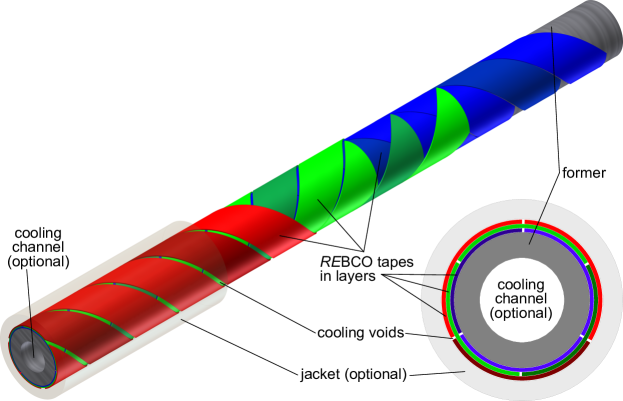
Figure 1: Schematic drawing of a CORC cable. REBCO tapes are tightly wound around a round former with a small diameter. The winding direction between the layers is reversed. The cable can optionally be fitted with a jacket of structural material for increased mechanical stabilization and with a hollow former for forced flow cooling. Picture from [16].

In CORC cables, the REBCO tapes are wound, with the superconducting layer in compression, to small diameters. This is possible without major reduction of their current carrying capabilities due to winding angles close to $45\text{\,}\mathrm{\SIUnitSymbolDegree}$, symmetrically distributing the winding strains onto the a-axis (100 direction) and b-axis (010 direction) of all REBCO crystals’ unit cells. This arrangement suppresses the impact of the winding strain on the current carrying capabilities, the so called reversible strain effect of the superconductor tapes [17]. However, even though the tapes are wound around the former in different winding directions, the transposition of the REBCO tapes in the CORC cable concept is only partial. This makes the response of CORC cables to swiftly changing currents highly interesting. The periodically changing orientation (due to the winding) of the REBCO tapes makes the cable’s current depending on the field component with the strongest critical current degradation. This however has two benefits in applications. Firstly, the field dependence of CORC cables is isotropic, the position in e.g. a solenoid magnet is of no importance. Secondly, the engineering current density $J_{\textrm{e}}$ of CORC cables is expected to increase rapidly with enhanced pinning, likely without an increase in conductor cost. In the following, a CORC cable sample is experimentally characterized in detail.

2 Experimental

2.1 Sample parameters

The investigated CORC cable sample was produced by Advanced Conductor Technologies. It was of $1.16\text{\,}\mathrm{m}$ length and consisted of 15, $4\text{\,}\mathrm{mm}$ wide SuperPower REBCO tapes stabilized with $20\text{\,}\mathrm{\SIUnitSymbolMicro m}$ thick layers of copper (Cu) plating on both sides (SCS4050). The tapes were arranged in five layers (three tapes per layer) and were wound around a round former of $5.5\text{\,}\mathrm{mm}$ diameter with a winding angle of ca. $45\mathrm{°}$. The former was a conventional stranded power cable which has been soldered into the terminations of the CORC cable sample. It provided mechanical and electrical stabilization. Three pairs of voltage taps were soldered to the REBCO tapes of the the outer layer and one pair was attached to the copper terminations of the sample. All sample parameters are summarized in table 1.

Table 1: Parameters of the investigated CORC cable sample.

parameter	CORC cable sample
sample length	$1.16\text{\,}\mathrm{m}$ including terminations, $0.96\text{\,}\mathrm{m}$ between terminations
superconductor	$4\text{\,}\mathrm{mm}$ wide, copper stabilized from SuperPower (SCS4050) - no advanced pinning
average tape $I_{\textrm{c}}$	$127.57\text{\,}\mathrm{A}$ at $77\text{\,}\mathrm{K}$, s.f. and $161.42\text{\,}\mathrm{A}$ at $4.2\text{\,}\mathrm{K}$, $12\text{\,}\mathrm{T}$
number of tapes	15 tapes in 5 layers (3 tapes per layer)
twist pitch $\tau$	$17\text{\,}\mathrm{mm}$
termination	all tapes individually soldered to cone shaped copper contacts
mechanical stabilization	stranded insulted former (power cable) with $5.5\text{\,}\mathrm{mm}$ diameter
electrical stabilization	$20\text{\,}\mathrm{\SIUnitSymbolMicro m}$ thick Cu stabilization of the tapes + Cu in the strands of former
voltage tap pairs	3 pairs at tapes in the outer layer + 1 pair at the copper contacts (the terminations)

The average critical current of the used REBCO tapes was determined after the field- and temperature dependent experiments by characterizing tapes from the same batch at $77\text{\,}\mathrm{K}$, self-field and at $4.2\text{\,}\mathrm{K}$, $12\text{\,}\mathrm{T}$. The field was applied perpendicular to the tape surface.

2.2 Measurement procedure

In a five step approach, the CORC cable sample’s performance was investigated at different transverse mechanical loads, magnetic background fields and temperatures.

• Critical current measurements at $77\text{\,}\mathrm{K}$, self-field in a liquid nitrogen bath (subsection 3.1).

• Temperature variable measurements at self-field conditions utilizing the variable temperature insert of the FBI (force - field - current) test facility (subsection 3.2).

• Impact of transverse mechanical loads generated by Lorentz forces in magnetic fields cycles of $212\text{\,}\mathrm{T}$. Degradations due to the increasing Lorentz forces will be made visible in these measurements by comparing the obtained critical currents of different load cycles (subsection 3.3).

• Critical current measurements at different fields and temperatures to determine the magnetic field and temperature dependence of CORC cables. The gained data is compared with single tape data published by the superconductor’s manufacturer (subsection 3.4).

• Response of the CORC cable sample to rapidly changing currents by measuring the voltage drop over the whole cable at a current ramp rate of $8.3\text{\,}\mathrm{kA}\text{\,}{\mathrm{s}}^{-1}$ (subsection 3.5).

2.3 Test setup

The field- and temperature dependent characterizations were performed using the FBI superconductor test facility of the Institute for Technical Physics (ITEP) of the Karlsruhe Institute of Technology (KIT) [18]. The test facility consisted of:

Current source:

A low noise DC power supply provided up to $10\text{\,}\mathrm{kA}$ of current to the sample. The measurements were performed at quasi-constant current; the current was increased slowly with a ramp rate of $20\text{\,}\mathrm{A}\text{\,}{\mathrm{s}}^{-1}$ from step to step. On each of the steps, the current was kept constant while the voltages were measured using low noise nano-voltmeters.

Magnet:

A superconducting split coil magnet delivered magnetic background fields up to $12\text{\,}\mathrm{T}$. The field was orientated perpendicular to the sample axis and the current. Approximately 4 transposition lengths of the sample were inside the $70\text{\,}\mathrm{mm}$ long high field region (field deviation less than $3\text{\,}\mathrm{\char 37\relax}$ from the peak value). Above and below the magnet, there were current leads connecting the sample to the power supply.

Variable temperature insert:

In the variable temperature insert, the central $100\text{\,}\mathrm{mm}$ of the sample were heated with heating foils while being thermally insulated from the helium bath with glass-fiber-reinforce-plastics (GFRP) G10 “cryostat”. The heated section of the sample and the high field region of the magnet were aligned. The heating system fitted tightly around the sample and was sealed with bees wax and adhesive tape at the upper and lower end to minimizes helium boil off. This system has been shown to exhibit fast response (less than $1\text{\,}\mathrm{min}$) and stable temperature, however there was a temperature gradient. The temperature gradient, as demonstrated on a CICC dummy, was low in longitudinal direction and was pronounced in radial direction [19]. As it was not possible to place temperature sensors on the CORC cable’s inside, its temperature distribution was therefore simulated (subsection 2.4). There were two Cernox temperature sensors in direct contact with the sample’s surface, their average was used as input for the model and is referred to as the surface temperature $T_{\textrm{surface}}$. The CORC cable sample equipped with the variable temperature insert is shown in figure 2.

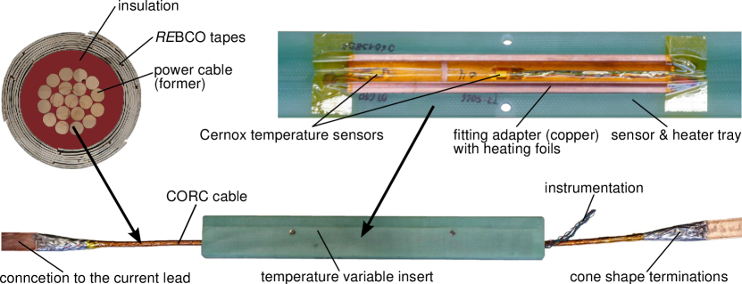
Figure 2: CORC cable sample in the variable temperature insert used in the magnetic field- and temperature dependent measurements. Picture from [6, 16].

2.4 Temperature distribution of the Conductor on Round Core cable

The heated section of the sample was modeled in full scale in 3D using the direction- and temperature dependent thermal conductivities of all constituent materials as shown in figure 3 with the commercial software package “Comsol” [20].

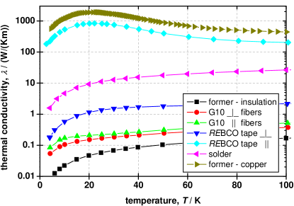
Figure 3: Thermal conductivity of the CORC cable sample’s constituent materials. Data from [21, 22, 16].

In the model, temperature sources (the average of the two Cernox sensors: surface temperature $T_{\textrm{surface}}$) and temperature sinks (the helium bath: $4.2\text{\,}\mathrm{K}$) were imposed as boundary conditions. For optimal resolution, different mesh configurations were used. The REBCO tapes were netted with a mapped mesh allowing the placement of several nodes within the width of each tape’s superconducting layer. A free tetradic mesh, with much lower node density, was used in the variable temperature insert. This simulation method is shown schematically in figure 4.

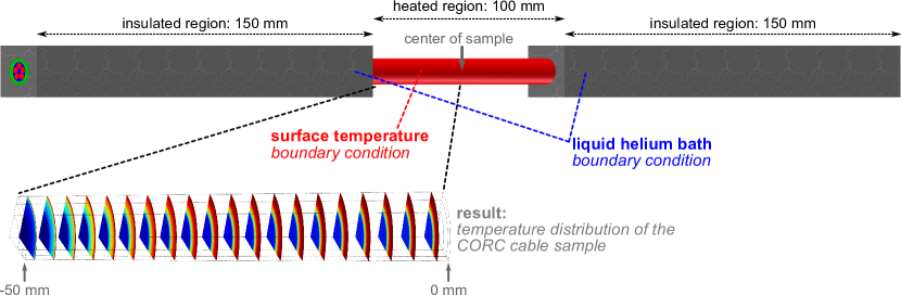
Figure 4: Schematic drawing of the FEM models used in the simulations of the temperature distribution of HTS cables in the variable temperature insert. An exemplary temperature distribution is shown as a color gradient from cold (blue) to hot (red). The figure is not up to scale.

With this method the temperature distribution was calculated for different surface temperatures $T_{\textrm{surface}}$. In regularly spaced positions along the sample (each $5\text{\,}\mathrm{mm}$), the temperatures of all tapes were averaged. In figure 5, this averaged cable temperature $T_{\textrm{average}}$ is shown from the center (position: $0\text{\,}\mathrm{mm}$) to the border of the heating section (position: $-50\text{\,}\mathrm{mm}$) for surface temperatures from $10\text{\,}\mathrm{K}$ to $100\text{\,}\mathrm{K}$.

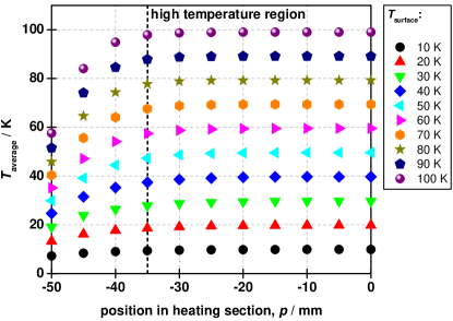
Figure 5: Simulated temperature distribution of the CORC cable sample. The average temperature of the cable $T_{\textrm{average}}$ is shown at different positions in the heating section from the border (position: $-50\text{\,}\mathrm{mm}$) to the center (position: $0\text{\,}\mathrm{mm}$) of the $100\text{\,}\mathrm{mm}$ long heating section)

From $-35\text{\,}\mathrm{mm}$ to the sample’s center (position: $0\text{\,}\mathrm{mm}$), the average temperature $T_{\textrm{average}}$ was stable. Due to the system’s symmetry this corresponded to the CORC sample’s central $70\text{\,}\mathrm{mm}$. There was a pronounced drop of the average temperature further away from the center (positions: $<-35\text{\,}\mathrm{mm}$ and $>35\text{\,}\mathrm{mm}$). The central $70\text{\,}\mathrm{mm}$ were therefore the variable temperature insert’s active zone and are referred to in the following as the sample’s high temperature region corresponding to the magnet’s high field region. Within the temperature range of interest (surface temperature: $<40\text{\,}\mathrm{K}$), the deviations from the average temperature in this zone were less than $\pm 3\text{\,}\mathrm{\char 37\relax}$. This distance of $70\text{\,}\mathrm{mm}$ was therefore a good assumption to define the working area of the variable temperature insert as well as the magnet. In this zone, magnetic field and temperature were assumed to be maximal as well as constant and the $70\text{\,}\mathrm{mm}$ were used to convert the measured voltages into electric fields regardless of the voltage taps’ separation. Outside these $70\text{\,}\mathrm{mm}$, the sample was at lower fields and/or temperatures. It was therefore away from the superconducting transition without any contribution to the measured sample voltages.

3 Results

3.1 LN₂ characterization

In the first step of the CORC cable characterization, the current carrying capabilities of the sample were measured in a liquid nitrogen (LN₂) bath at $77\text{\,}\mathrm{K}$ in self-field conditions. Due to the steep transitions and homogeneous contact resistances, a $1\text{\,}\mathrm{\SIUnitSymbolMicro V}\text{\,}{\mathrm{cm}}^{-1}$ criteria was used to determinate of the critical currents in all following investigations. As there was neither magnetic field nor heating, the actual distance between the voltage taps was used to convert voltages into electric fields. The critical currents gained from all available voltage taps are shown in table 2, subtracting any linear ohmic contributions.

Table 2: $77\text{\,}\mathrm{K}$ (LN₂ bath), self-field current carrying of the CORC cable sample for different voltage taps ($1\text{\,}\mathrm{\SIUnitSymbolMicro V}\text{\,}{\mathrm{cm}}^{-1}$ criteria). Linear ohmic contributions are subtracted.

voltage tap:	tap1	tap2	tap3	terminations
$I_{\textrm{c}}$:	$1752\text{\,}\mathrm{A}$	$1652\text{\,}\mathrm{A}$	$1757\text{\,}\mathrm{A}$	$1638\text{\,}\mathrm{A}$

Voltage taps are only available at the outer three of the 15 REBCO tapes of the sample. Even these tapes transition at slightly different currents ($16521757\text{\,}\mathrm{A}$). Thus, the voltage drop across the copper terminations (the sample’s contacts) is most relevant as it averages over the behavior of all tapes, it is therefore used for the determination of the samples current carrying capabilities in all following experiments. Using the copper contacts’ voltage taps, the $77\text{\,}\mathrm{K}$, self-field the critical current of sample is $I_{\textrm{c}}\left($77\text{\,}\mathrm{K}$,\textrm{self-field}\right)=$1638\text{\,}\mathrm{A}$$ (see [23, p. 7]). The used superconductor tapes have an average $77\text{\,}\mathrm{K}$, self-field current of $127.57\text{\,}\mathrm{A}$ (measured in LN₂ bath on several tapes of the same REBCO tape batch), resulting in a design current ($15\times$ $127.57\text{\,}\mathrm{A}$) of the CORC cable of $1913\text{\,}\mathrm{A}$. The sample’s self-field degradation is $14.38\text{\,}\mathrm{\char 37\relax}$.

3.2 Temperature dependence

In the second step, the temperature dependence of the current carrying capabilities of the CORC cable sample was investigated at self-field conditions using the variable temperature insert. Critical currents were determined with a $1\text{\,}\mathrm{\SIUnitSymbolMicro V}\text{\,}{\mathrm{cm}}^{-1}$ criteria using the voltage taps at the copper contacts. A distance of $70\text{\,}\mathrm{mm}$ (the variable temperature insert’s high temperature region) was used to convert voltages into electric fields. Outside this region, the temperatures dropped quickly therefore avoiding any influence on the measured voltages. The current bypass through the copper in the former (the power cable) was determined to be negligible. In the sample’s former, there were $19$ copper strands of $0.75\text{\,}\mathrm{mm}$ diameter resulting in a total copper cross sectional area of $8.32\text{\times}{10}^{-9}\text{\,}{\mathrm{m}}^{2}$. With a residual resistivity ratio (RRR) of $100$ and a specific resistivity of copper at room temperature of $16.78\text{\,}\mathrm{n\SIUnitSymbolOhm}\text{\,}\mathrm{m}$, the total electrical resistivity between the terminations ($0.96\text{\,}\mathrm{m}$ separation) was $19\text{\,}\mathrm{\SIUnitSymbolMicro\SIUnitSymbolOhm}$ at operating conditions. This resulted in a current bypass of $3.6\text{\,}\mathrm{A}$ at ten times the critical electric field (voltage of $7\text{\times}{10}^{-5}\text{\,}\mathrm{V}$ over the whole sample). This calculation does not account for the contact resistance between the terminations and the former and as the former was clamped into the terminations and fixed with a stainless steel screw, thus this in an upper limit of the real current bypass. The simulated temperature distribution of the sample (figure 5) was averaged in the high temperature region leading to the the average cable temperatures $T_{\textrm{average}}$ for the experiment’s measured surface temperatures $T_{\textrm{surface}}$. These temperatures as well as the statistic (derived from the averaging) and the systematic (from the temperature measurement) uncertainties are given in table 3.

Table 3: Sample surface temperatures $T_{\textrm{surface}}$, average sample temperatures $T_{\textrm{avg}}$, statistic and systematic uncertainty derived from the FEM model of the CORC sample.

surface temperature, $T_{\textrm{surface}}$	average cable temperature, $T_{\textrm{average}}$	statistic uncertainty	systematic uncertainty
$15.2\text{\,}\mathrm{K}$	$14.8\text{\,}\mathrm{K}$	$\pm 0.3\text{\,}\mathrm{K}$	$\pm 0.5\text{\,}\mathrm{K}$
$21.4\text{\,}\mathrm{K}$	$20.8\text{\,}\mathrm{K}$	$\pm 0.5\text{\,}\mathrm{K}$	$\pm 0.7\text{\,}\mathrm{K}$
$33.5\text{\,}\mathrm{K}$	$32.7\text{\,}\mathrm{K}$	$\pm 0.7\text{\,}\mathrm{K}$	$\pm 1.1\text{\,}\mathrm{K}$
$42.1\text{\,}\mathrm{K}$	$41.2\text{\,}\mathrm{K}$	$\pm 0.9\text{\,}\mathrm{K}$	$\pm 1.4\text{\,}\mathrm{K}$
$44.6\text{\,}\mathrm{K}$	$43.7\text{\,}\mathrm{K}$	$\pm 0.8\text{\,}\mathrm{K}$	$\pm 1.5\text{\,}\mathrm{K}$
$49.9\text{\,}\mathrm{K}$	$59.1\text{\,}\mathrm{K}$	$\pm 0.8\text{\,}\mathrm{K}$	$\pm 1.6\text{\,}\mathrm{K}$
$55.9\text{\,}\mathrm{K}$	$55.0\text{\,}\mathrm{K}$	$\pm 0.8\text{\,}\mathrm{K}$	$\pm 1.8\text{\,}\mathrm{K}$
$62.4\text{\,}\mathrm{K}$	$61.5\text{\,}\mathrm{K}$	$\pm 0.8\text{\,}\mathrm{K}$	$\pm 1.9\text{\,}\mathrm{K}$
$69.7\text{\,}\mathrm{K}$	$68.8\text{\,}\mathrm{K}$	$\pm 0.6\text{\,}\mathrm{K}$	$\pm 2.1\text{\,}\mathrm{K}$
$73.7\text{\,}\mathrm{K}$	$72.7\text{\,}\mathrm{K}$	$\pm 0.7\text{\,}\mathrm{K}$	$\pm 2.1\text{\,}\mathrm{K}$
$75.7\text{\,}\mathrm{K}$	$74.7\text{\,}\mathrm{K}$	$\pm 0.6\text{\,}\mathrm{K}$	$\pm 2.1\text{\,}\mathrm{K}$
$77.8\text{\,}\mathrm{K}$	$76.9\text{\,}\mathrm{K}$	$\pm 0.5\text{\,}\mathrm{K}$	$\pm 2.2\text{\,}\mathrm{K}$

The measured cable critical current $I_{\textrm{c}}$ depending on the average temperature $T_{\textrm{average}}$ is compared in figure 6 with the single REBCO tape temperature dependence published by the manufacturer [24]. Single tapes are extrapolated by normalizing to the CORC cable’s $77\text{\,}\mathrm{K}$ current carrying capabilities (from the LN₂ bath, self-field experiment in subsection 3.1). Increased self-fields at lower temperatures and higher cable currents are not considered in this extrapolation.

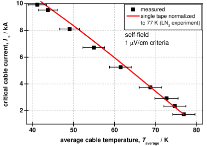
Figure 6: Temperature dependence of the critical current of the CORC cable sample (black dots) and extrapolated REBCO tapes from SuperPower (red line) at self-field conditions. The CORC cable is measured with the variable temperature insert of the FBI test facility. Its average temperature is calculated using the simulated temperature distribution presented in figure 5. Single tape temperature dependence from [24], normalized to the cables $77\text{\,}\mathrm{K}$ current carrying capabilities (LN₂ experiment, see subsection 3.1).

The temperature variable CORC cable measurement and the extrapolated single tape data are in good agreement within the uncertainty of the temperature determination (combining statistic and systematic uncertainties, see table 3). In the investigated temperature range of $4077\text{\,}\mathrm{K}$, the temperature dependence is linear for the single tapes and nearly linear for the CORC cable measurement.

3.3 Magnetic field cycles

In the third step, the CORC cable sample was checked for degradation of the current carrying capabilities due to high transverse mechanical loads. This was achieved through cycling of the magnetic background field, currents and therefore transverse loads generated by the Lorentz force. The magnetic background field was increased from $2\text{\,}\mathrm{T}$ (due to limitations of the current source, maximum current is $10\text{\,}\mathrm{kA}$) to $12\text{\,}\mathrm{T}$. Every $2\text{\,}\mathrm{T}$, the critical current was measured at $4.2\text{\,}\mathrm{K}$ using a $1\text{\,}\mathrm{\SIUnitSymbolMicro V}\text{\,}{\mathrm{cm}}^{-1}$ criteria with the voltage tap pair at the copper contacts and assuming $70\text{\,}\mathrm{mm}$ (magnet’s high field region) to calculate electric fields while subtracting any linear ohmic contribution.

The critical current index values (n-values) of all superconducting transitions are in the $3955\text{\,}$ range. N-values are obtained between the critical electric field ($1\text{\,}\mathrm{\SIUnitSymbolMicro V}\text{\,}{\mathrm{cm}}^{-1}$) and ten times the critical electric field ($10\text{\,}\mathrm{\SIUnitSymbolMicro V}\text{\,}{\mathrm{cm}}^{-1}$) using nonlinear fitting and assuming power law behavior. The current carrying capabilities are identical on the first (black curves in figure 7) to the following field cycle (red curves). During the field cycles, the maximal transverse Lorentz forces (per sample length) on the CORC cable sample of $31.4\text{\,}\mathrm{kN}\text{\,}{\mathrm{m}}^{-1}$ occur during the critical current measurements at $12\text{\,}\mathrm{T}$ magnetic background field. No irreversible degradation of the current carrying capabilities is observed, the sample’s performance remains constant during all field cycles.

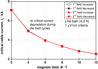
Figure 7: Critical current measurements at increasing and decreasing magnetic background fields of the CORC cable sample. There is no degradation of the sample’s current carrying capabilities in different magnetic field cycles.

3.4 Magnetic field- and temperature dependence

In the fourth step, the magnetic field- and temperature dependence of the current carrying capabilities of the CORC cable sample were determined. The sample’s critical currents were measured for sample surface temperatures from $4.2\text{\,}\mathrm{K}$ to $51.5\text{\,}\mathrm{K}$ in the magnetic field range from $2\text{\,}\mathrm{T}$ to $12\text{\,}\mathrm{T}$. The critical currents were measured each $2\text{\,}\mathrm{T}$ for different cable surface temperatures with a $1\text{\,}\mathrm{\SIUnitSymbolMicro V}\text{\,}{\mathrm{cm}}^{-1}$ criteria at the copper contacts’ voltage tap pair. A distance of $70\text{\,}\mathrm{mm}$ (high temperature & high field region) was utilized to calculate electric fields while subtracting the linear ohmic contribution of the contact resistance. The same sample surface temperature steps were used in the whole magnetic field range.

3.4.1 Behavior of the sample

Regardless of magnetic field or temperature, the shape of the transitions from superconducting state to normal conduction remain similar; all transitions are steep. In figure 8, two exemplary electric field vs. current curves are shown: high temperature (left: a) and high magnetic background field (right: b). All data is as measured, a distance of $70\text{\,}\mathrm{mm}$ is used to calculate electric fields and linear contributions are not subtracted. Voltage taps on the REBCO tape exhibit minimal linear ohmic contributions, while at the copper contact these are due to the contact resistances more pronounced. The overall contact resistance is $1.6\text{\,}\mathrm{n\SIUnitSymbolOhm}$, it is obtained by comparing the linear part’s slope of the electric field vs. cable current curves at the voltage taps on the REBCO tapes with the behavior of the whole cable, measured at the copper terminations. Using the previously described calculation method (see subsection 3.2), the current bypass is negligible and remains below $4\text{\,}\mathrm{A}$ even at ten times the critical electric field.

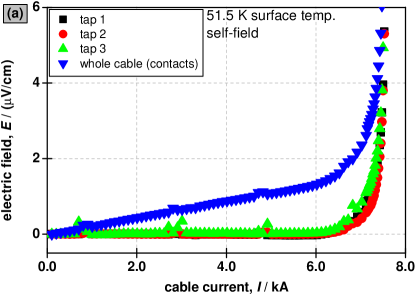
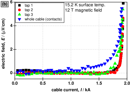
Figure 8: Exemplary electric field vs. current curves for the superconducting transitions in the field- and temperature dependent measurement of the CORC cable sample: high surface temperature (left: a) and high magnetic background field (right: b).

Similar behavior was obtained for all superconducting transitions of this sample, implying constant performance in the whole magnetic field- and temperature range. The sample’s electrical stabilization is sufficient as no significant increase of the cable temperature is observed during superconducting transitions even close to the maximal current of the test facility ($10\text{\,}\mathrm{kA}$).

3.4.2 Critical current vs. magnetic field and surface temperature

The obtained critical cable currents (y-axis) at different magnetic background fields (x-axis) and sample surface temperatures (in the legend) are shown in figure 9. The obtained field dependent curves of different sample surface temperatures are regularly spaced and follow a reciprocal dependence ($I_{\textrm{c}}=\frac{1}{\left(\alpha+\beta\cdot B\right)}$).

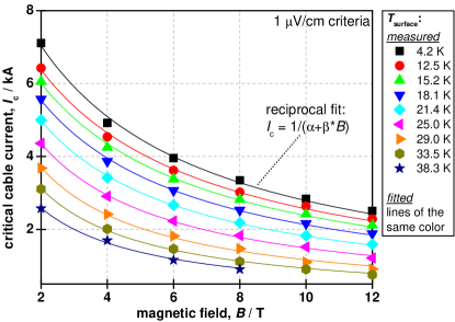
Figure 9: Magnetic field- and surface temperature $T_{\textrm{surface}}$ dependent measurements of the CORC cable sample. The measured data (points) is fitted with reciprocal functions (lines).

3.4.3 Critical current vs. magnetic field and average cable temperature

Using the simulated temperature dependence of the CORC cable sample (subsection 2.4) and averaging the temperature of the tapes for each position, an average cable temperature was calculated for the different sample surface temperatures. Surface temperatures $T_{\textrm{surface}}$, average temperatures $T_{\textrm{average}}$ as well as the statistic (derived from the averaging) and the systematic (from the temperature measurement) uncertainties are given in table 3. The critical currents at different magnetic background fields (x-axis) and effective temperatures (in the legend) are compared with the extrapolated current carrying capabilities of single REBCO tapes. The average $4.2\text{\,}\mathrm{K}$, $12\text{\,}\mathrm{T}$ current carrying capabilities of the sample’s REBCO tapes ($161.42\text{\,}\mathrm{A}$ measured on tapes of the same batch, see table 1) are extrapolated to different fields and temperatures using the single tape field- and temperature dependence factors $I_{\textrm{c}}(T,B_{\perp})/I_{\textrm{c}}($4.2\text{\,}\mathrm{K}$,$12\text{\,}\mathrm{T}$_{\perp})$ published by the REBCO tapes’ manufacturer [24]. The magnetic background field as well as the cable’s self-field are considered. Measured data (points) and extrapolated data (lines) are shown in figure 10.

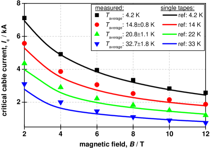
Figure 10: Field- and average cable temperature $T_{\textrm{average}}$ dependent measurements of the CORC cable sample: measurements (points) and extrapolated single tape data (lines). The $4.2\text{\,}\mathrm{K}$, $12\text{\,}\mathrm{T}$ current carrying capabilities of REBCO tapes from the same batch are extrapolated to different fields and temperatures using the single tape field- and temperature dependence published by the manufacturer [24].

Measured and extrapolated data are in good agreement, with the CORC cable currents being slightly higher than the extrapolated REBCO tapes in the majority of field and temperature combinations. At $4.2\text{\,}\mathrm{K}$, and $12\text{\,}\mathrm{T}$$\;\perp$ (perpendicular magnetic background field) the CORC cable sample carries $2.53\text{\,}\mathrm{kA}$ corresponding to a linear (one dimensional) current density of $422\text{\,}\mathrm{A}\mathrm{/}\mathrm{c}\mathrm{m}\mathrm{-}\mathrm{w}\mathrm{i}\mathrm{d}\mathrm{t}\mathrm{h}$. This perfectly matches the performance reported by the manufacturer reported for this type of conductor (SCS4050):$425\text{\,}\mathrm{A}\mathrm{/}\mathrm{c}\mathrm{m}\mathrm{-}\mathrm{w}\mathrm{i}\mathrm{d}\mathrm{t}\mathrm{h}$ at $4.2\text{\,}\mathrm{K}$, $12\text{\,}\mathrm{T}$$\;\perp$ [24, p. 8][25]). This clearly shows that the REBCO tapes’ current carrying capabilities are fully utilized in the CORC cable concept and that the sample has a temperature- and magnetic background field dependence identical to single tapes.

3.5 High current ramp rates

In the fifth step, the response of the CORC cable sample to rapidly changing currents was investigated to simulate the fast charging or discharging of magnets. Using a low noise signal amplifier and a data acquisition system, the voltage across the CORC cable sample’s copper contacts was measured during the fast ramping of the current (current ramp rate of $8.3\text{\,}\mathrm{kA}\text{\,}{\mathrm{s}}^{-1}$). The measurement was done at self-field conditions and a cable temperature of $4.2\text{\,}\mathrm{K}$. At the boundary conditions, the sample’s critical current was above the test facilities maximum current, the measured voltage was therefore the result of the contact resistance ($1.6\text{\,}\mathrm{n\SIUnitSymbolOhm}$, see subsection 3.4.1) as well as the sample’s impedance. The measured voltages (full symbols) and the voltage without the contribution of the contact resistance (hollow symbols) as well as the current ramping (line) are shown in figure 11.

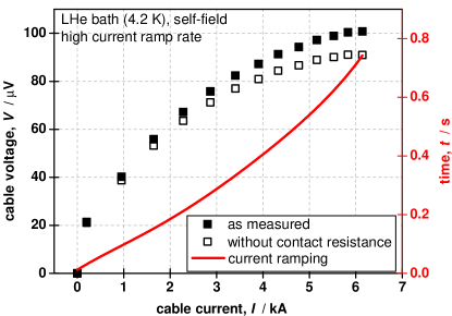
Figure 11: High current ramp rates on CORC cables. Current of the sample ($4.2\text{\,}\mathrm{K}$, self-field conditions) is increased at a ramp rate of $8.3\text{\,}\mathrm{kA}\text{\,}{\mathrm{s}}^{-1}$. The voltage drop between the copper terminations is measured with a fast data acquisition system. The measured voltages (full symbols) and the voltage without the contribution of the contact resistance (hollow symbols) as well as the current ramping (line) are shown.

No voltage spikes are observed. The maximal occurring voltage over the whole sample (length of $0.96\text{\,}\mathrm{m}$ between the terminations, see table 1) is $1.008\text{\times}{10}^{-4}\text{\,}\mathrm{V}$ and $0.910\text{\times}{10}^{-4}\text{\,}\mathrm{V}$ subtracting the contribution of the contact resistance. Combined with the average current ramp rate of $8.3\text{\,}\mathrm{kA}\text{\,}{\mathrm{s}}^{-1}$, the sample’s inductance is of the order of $1\text{\times}{10}^{-8}\text{\,}\mathrm{H}$. The corresponding electric field even remains below the critical electric field of $1\text{\,}\mathrm{\SIUnitSymbolMicro V}\text{\,}{\mathrm{cm}}^{-1}$. At this voltage the current bypass through the copper former is still negligible, it remains below $5.3\text{\,}\mathrm{A}$ using the previously described calculation method (see subsection 3.2). The investigated CORC cable sample is able to withstand fast changes of its current.

4 Discussion and conclusion

The temperature and magnetic field depended current carrying capabilities of a Conductor on Round Core (CORC) cable with 15 SuperPower SCS4050 (no advanced pinning) tapes (3 per layer) have been investigated in detail using the FBI test facility of the Institute for Technical Physics (ITEP) of the Karlsruhe Institute of Technology (KIT). A variable temperature insert locally heated the CORC cable sample. This system’s temperature distribution was modeled in fully scale with FEM using the direction and temperature dependent thermal conductivities of the sample’s constituent materials. Constant and maximal temperatures were found in a $70\text{\,}\mathrm{mm}$ long region, the high temperature region corresponding to the high temperature region of the magnet. Outside this region, temperatures and magnetic fields dropped quickly and $70\text{\,}\mathrm{mm}$ were therefore used to convert voltages into electric fields in all temperature- and magnetic field dependent measurements. The CORC cable sample’s superconducting transitions were steep and of high n-value ($3955\text{\,}$ range) allowing the use of a $1\text{\,}\mathrm{\SIUnitSymbolMicro V}\text{\,}{\mathrm{cm}}^{-1}$ criteria. The current bypass through the copper in the former is negligible. The current carrying capabilities of the REBCO tapes from the same batch have been determined (on several single tapes, not assembled to a cable). In average, each of the $4\text{\,}\mathrm{mm}$ wide tapes carried $127.57\text{\,}\mathrm{A}$ at $77\text{\,}\mathrm{K}$, self-field and $161.42\text{\,}\mathrm{A}$ at $4.2\text{\,}\mathrm{K}$ $12\text{\,}\mathrm{T}$.

The investigations were performed in five steps. In the first step the sample’s $77\text{\,}\mathrm{K}$ (LN₂ bath), self-field current was determined to $16521757\text{\,}\mathrm{A}$ depending on the used voltage tap. Due to these differences, all following experiments use the voltage taps on the copper contacts (the sample’s terminals) the averages over the behavior of all tapes. Referring to this voltage tap, the CORC cable carries $1638\text{\,}\mathrm{A}$; compared with its design value of $1913\text{\,}\mathrm{A}$, this corresponded to a self-field degradation of only $14.38\text{\,}\mathrm{\char 37\relax}$. In the second step, the sample’s self-field temperature dependence was determined in the $4277\text{\,}\mathrm{K}$ range and compared with extrapolated single tapes. The CORC cable’s temperature is derived by combining the simulated temperature distribution with the measured sample surface temperature. The single tape extrapolation uses the tapes’ temperature dependence as published by the manufacturer and normalizes with the $77\text{\,}\mathrm{K}$ (LN₂ bath), self-field cable current. Measured and extrapolated data are in good agreement within the uncertainty of the determination of the average cable temperature. In the third step, the sample’s stability against high transverse mechanical loads was investigated by repeatedly cycling the magnetic background field between $2\text{\,}\mathrm{T}$ and $12\text{\,}\mathrm{T}$. No degradation of its current carrying capability was observed during the magnetic field cycles with maximal transverse Lorentz forces (per sample length) of up to $31.4\text{\,}\mathrm{kN}\text{\,}{\mathrm{m}}^{-1}$. In the fourth step, the magnetic field- and temperature dependence of the current carrying capabilities of the CORC cable sample were determined and compared with extrapolated single tape data. The extrapolation uses the average $4.2\text{\,}\mathrm{K}$, $12\text{\,}\mathrm{T}$ current carrying capabilitiesREBCO tapes from the same batch and the field- and temperature dependence factors $I_{\textrm{c}}(T,B_{\perp})/I_{\textrm{c}}($4.2\text{\,}\mathrm{K}$,$12\text{\,}\mathrm{T}$_{\perp})$ published by the tapes’ manufacturer. Measured and extrapolated data are in good agreement, with the CORC cable’s currents being slightly higher than the extrapolated REBCO tapes in the majority of field and temperature combinations. At $4.2\text{\,}\mathrm{K}$, and $12\text{\,}\mathrm{T}$$\;\perp$ (perpendicular magnetic background field) the sample has a critical current of $2.53\text{\,}\mathrm{kA}$ corresponding to a current density of $422\text{\,}\mathrm{A}\mathrm{/}\mathrm{c}\mathrm{m}\mathrm{-}\mathrm{w}\mathrm{i}\mathrm{d}\mathrm{t}\mathrm{h}$ which perfectly matches the performance reported by the manufacturer. This clearly shows that the sample’s temperature- and field dependence is identical to that of its constituent REBCO tapes as well as that tapes’ current carrying capabilities are fully utilized. In the fifth step, the CORC cable’s response to rapidly changing currents was investigated. No voltage spikes were observed at current ramp rates of $8.3\text{\,}\mathrm{kA}\text{\,}{\mathrm{s}}^{-1}$, the inductance is of the order of $1\text{\times}{10}^{-8}\text{\,}\mathrm{H}$. Subtracting the contact resistance of the copper terminations ($1.6\text{\,}\mathrm{n\SIUnitSymbolOhm}$), the electric field remains below the critical electric field of $1\text{\,}\mathrm{\SIUnitSymbolMicro V}\text{\,}{\mathrm{cm}}^{-1}$. There was no irreversible reduction of the CORC cable’s performance in any of the experimental steps.

These finding clearly show CORC cables being very promising candidates as conductor in high field or fusion magnets.

References

- [1] W Goldacker, R Nast, G Kotzyba, S I Schlachter, a Frank, B Ringsdorf, C Schmidt, and P Komarek. High current DyBCO-ROEBEL Assembled Coated Conductor (RACC). Journal of Physics: Conference Series, 43:901–904, June 2006.
- [2] N J Long. HTS Roebel cables. In HTS4Fusion Conductor Workshop, KIT CN, Karlsruhe, 2011.
- [3] S I Schlachter, W Goldacker, F Grilli, R Heller, and A Kudymow. Coated Conductor Rutherford Cables (CCRC) for High-Current Applications: Concept and Properties. IEEE Transactions on Applied Superconductivity, 21(3):3021–3024, June 2011.
- [4] A Kario, M Vojenciak, F Grilli, A Kling, B Ringsdorf, U Walschburger, S I Schlachter, and W Goldacker. Investigation of a Rutherford cable using coated conductor Roebel cables as strands. Superconductor Science and Technology, 26(8):085019, August 2013.
- [5] D C van der Laan. YBa2Cu3O7- coated conductor cabling for low ac-loss and high-field magnet applications. Superconductor Science and Technology, 22(6):065013, June 2009.
- [6] D C van der Laan, X F Lu, and L F Goodrich. Compact GdBa2Cu3O7- coated conductor cables for electric power transmission and magnet applications. Superconductor Science and Technology, 24(4):042001, April 2011.
- [7] D C van der Laan, L F Goodrich, and T J Haugan. High-current dc power transmission in flexible RE-Ba2Cu3O7- coated conductor cables. Superconductor Science and Technology, 25(1):014003, January 2012.
- [8] D C van der Laan, P D Noyes, G E Miller, H W Weijers, and G P Willering. Characterization of a high-temperature superconducting conductor on round core cables in magnetic fields up to 20 T. Superconductor Science and Technology, 26(4):045005, April 2013.
- [9] M Takayasu, J V Minervini, and L Bromberg. US patent: Superconductor Cable (patent number: 8 437 819 B2), 2009.
- [10] M Takayasu, L Chiesa, L Bromberg, and J V Minervini. Cabling Method for High Current Conductors Made of HTS Tapes. Applied Superconductivity, IEEE Transactions on, 21(3):2340–2344, 2011.
- [11] M Takayasu, J V Minervini, L Bromberg, M K Rudziak, and T Wong. Investigation of Twisted Stacked-Tape Cable Conductor. AIP Conference Proceedings, 1435:273–280, 2012.
- [12] M Takayasu, L Chiesa, L Bromberg, and J V Minervini. HTS twisted stacked-tape cable conductor. Superconductor Science and Technology, 25(1):014011, January 2012.
- [13] L Chiesa, N C Allen, and M Takayasu. Electromechanical Investigation of 2G HTS Twisted Stacked-Tape Cable Conductors. IEEE Transactions on Applied Superconductivity, 24(3):6600405, June 2014.
- [14] G Celentano, G De Marzi, F Fabbri, L Muzzi, G Tomassetti, A Anemona, S Chiarelli, M Seri, A Bragagni, and A della Corte. Design of an Industrially Feasible Twisted-Stack HTS Cable-in-Conduit Conductor for Fusion Application. IEEE Transactions on Applied Superconductivity, 24(3):4601805, 2014.
- [15] D Uglietti, R Wesche, and P Bruzzone. Fabrication Trials of Round Strands Composed of Coated Conductor Tapes. IEEE Transactions on Applied Superconductivity, 23(3):4802104, 2013.
- [16] C Barth. High Temperature Superconductor Cable Concepts for Fusion Magnets. KIT Scientific Publishing, Karlsruhe, 1. edition, 2013.
- [17] D C van der Laan, D Abraimov, A A Polyanskii, D C Larbalestier, J F Douglas, R Semerad, and M Bauer. Anisotropic in-plane reversible strain effect in Y0.5 Gd0.5Ba2Cu3O7coated conductors. Superconductor Science and Technology, 24(11):115010, November 2011.
- [18] C M Bayer, C Barth, P V Gade, K Weiss, and R Heller. FBI Measurement Facility for High Temperature Superconducting Cable Designs. IEEE Transactions on Applied Superconductivity, 24(3):9500604, 2014.
- [19] C Barth, M Takayasu, N Bagrets, C M Bayer, K-P Weiss, and C Lange. Temperature- and Field Dependent Characterization of a Twisted Stacked-Tape Cable. Superconductor Science and Technology, 28(4):045015, 2015.
- [20] COMSOL Inc. COMSOL Multiphysicstextsuperscript®.
- [21] N Bagrets, C Barth, and K Weiss. Low Temperature Thermal and Thermo-Mechanical Properties of Soft Solders for Superconducting Applications. IEEE Transactions on Applied Superconductivity, 24(3):7800203, 2014.
- [22] N Bagrets, W Goldacker, S I Schlachter, and C Barth. Thermal properties of 2G coated conductor cable materials. CRYOGENICS, 61:8–14, 2014.
- [23] C Barth, S Drotziger, W H Fietz, W Goldacker, R Heller, and K-P Weiss. Final-Report on Construction and test of DEMO relevant cables (WP12-DAS-01-T06). Technical report, EFDA Work Program 2012 Design Assessment Studies: Superconducting Magnets (WP12-DAS01-MAG), Karslruhe Institute of Technology, CN, Eggenstein-Leopoldshafen, 2012.
- [24] D W Hazelton. 2G HTS Conductors at SuperPower. In Low Temperature High Field Superconductor Workshop, Napa, 2012. SuperPower.
- [25] SuperPower. 2G HTS Wire Specifications. In: http://www.superpower-inc.com/system/files/SP_2G+Wire+Spec+Sheet_for+web_0509.pdf.