Cosmology and Gravitation: the grand scheme for High-Energy Physics

Abstract

These lectures describe how the Standard Model of cosmology ($\Lambda$CDM) has developped, based on observational facts but also on ideas formed in the context of the theory of fundamental interactions, both gravitational and non-gravitational, the latter being described by the Standard Model of high energy physics. It focuses on the latest developments, in particular the precise knowledge of the early Universe provided by the observation of the Cosmic Microwave Background and the discovery of the present acceleration of the expansion of the Universe. While insisting on the successes of the Standard Model of cosmology, we will stress that it rests on three pillars which involve many open questions: the theory of inflation, the nature of dark matter and of dark energy. We will devote one chapter to each of these issues, describing in particular how this impacts our views on the theory of fundamental interactions. More technical parts are given in italics. They may be skipped altogether.

0.1 A not so brief history of modern cosmology

Cosmology has been an enquiry of the human kind probably since the dawn of humanity. Modern cosmology was born in the early XX^th century with the bold move of Einstein and contemporaries to apply the equations of general relativity, the theory of gravity, to the whole Universe. This has led to many successes and/or suprises, the most notable of which being presumably the discovery of extra-galactic objects which recede from our own Galaxy, i.e. the discovery of the expansion of the Universe [Le27, Hu29]. This led to the development of the Big Bang theory, with the early Universe being a hot and dense medium (a prediction confirmed by the discovery of the cosmic microwave background by Penzias and Wilson in 1965 [PW65]), and thus a laboratory for studying elementary particles. A picture thus emerged in the 1970s, not only based on the theory of gravity, but also on non-gravitational interactions described by the Standard Model of high energy physics, which was being finalized at the same time (its experimental confirmation would take another 40 years and has culminated in the discovery of the Higgs particle in 2012).

A first success of the particle physics approach to cosmology has been the understanding of the abundancy of light elements in the 80s. This was the first quantitative success of cosmology. Meanwhile, the development of gauge symmetries and the understanding of the rôle of spontaneous symmetry breaking in fundamental interactions led the community to focus its attention on phase transitions in the early Universe, in particular associated with the quark-gluon transition, the breaking of the electroweak symmetry or even of the grand unified symmetry. It is in this context that, in the early 80s, the theory of inflation was proposed [St80, Gu81] to solve some of the mysteries of the standard Big Bang theory.

The theory of inflation included a model for the genesis of density fluctuations responsible for the formation of large scale structures, such as galaxies or clusters of galaxies: the quantum fluctuations during the exponential (de Sitter) expansion. But this implied the presence of fluctuations in the otherwise homogeneous and istropic Cosmic Microwave Background. Such fluctuations were observed by the COBE satellite, at the level of one part in 100 000. Generic models of inflation predicted also in a very elegant manner that space (not spacetime!) is flat, any spatial curvature being erased by the exponential expansion. According to Einstein’s equations, this implied that the average energy density in the Universe had the critical value $\rho_{c}\sim 10^{-26}{\rm kg}/{\rm m}^{3}$.

This was a prediction not supported by observation. It was known since the 1930s that there was a significant amont of non-luminous –or dark– matter in the Universe: in 1933, Fritz Zwicky, by studying the velocity distribution of galaxies in the Coma cluster, had identified that there was $400$ times more mass than expected from their luminosity. This had been confirmed by studying subsequently the rotation curves of many other galaxies. But the total of luminous and dark matter could not account for more than $30\%$ of the critical energy density (other components like radiation are subdominant at present times). Models of open inflation were even constructed to reconcile inflation with observation.

The clue came in 1999 [HZS98a, SCP99] when it was observed that the expansion of the Universe is presently accelerating. Since matter or radiation tend to decelerate the expansion, one has to resort to a new form of energy, named dark energy, to understand this acceleration. Was this the component which would provide the missing $70\%$ to account for a total energy density $\rho_{c}$ and thus a spatially flat Universe? The answer came from a more precise study of the fluctuations in the CMB through the space mission WMAP (and more recently Planck): they conclude indeed that these fluctuations are consistent with spatial flatness.

The latest cosmology results from the Planck mission, released this year, have confirmed the predictions of the simplest models of inflation, a rather remarkable feat since they are associated with dynamics active in the first fractions of seconds after the big bang, and they allow tu fully understand the imprints observed 350 000 years after the big bang.

We thus have at our disposal a Standard Model of cosmology which is sometimes compared with the Standard Model of high energy physics: in both cases, no major experimental/observational data seems to be in conflict with the Model. There is however one big difference. The Standard Model of cosmology rests on three “pillars” –inflation, dark matter, dark energy– which are very poorly known: we have at present no microscopic theory of inflation, and we ignore the exact nature of dark matter or dark energy.

For example, there are convincing arguments that dark matter is made of weakly interacting massive particles of a new type, and a large experimental programme has been set up to identify them. Their discovery would be of utmost importance because this would be the first sign of physics beyond the Standard Model of particle physics. But it remains a possibility –though not a favored one– to explain the observed facts through a modification of gravity at different scales (from galaxies to clusters and cosmological scales). Finally, axion dark matter would be a minimal extension fof the Standard Model, accounting for dark matter.

The discovery of the Higgs has provided us with the first example of a fundamental scalar field (at least fundamental at the scale where we observe it). this a welcome for cosmology since microscopic models of accleration of the expansion of the Universe –whether inflation or dark energy– make heavy use of such fields. They have the double advantage of being non-vanishing without breaking the symmetries of spacetime (like Lorentz symmetry) and of having the potential of providing an unclustered background. they also appear naturally in the context of extensions of the Standard Model, like supersymmetry or extra dimensions.

Scalar fields thus provide valuable toy models of inflation or dark energy. However, such toys models are difficult to implement into realistic high energy physics models because of the constraints existing on physics beyond the Standard Models of particle physics and cosmology.

In what follows, we will review the successes of the Standard Model of cosmology, focussing on the most recent results. And we will consider the three pillars of this Model —inflation, dark matter, dark energy– and identify the most pressing questions concerning these three concepts.

In what follows some more technical discussions are given in italics. They can be skipped altogether. Background material is also provided in Appendices, most of it being intended for the reader who wants to reproduce some of the more advanced results.

We start in this first Chapter with an introduction, partly historical, to the main concepts of cosmology.

0.1.1 Gravity governs the evolution of the Universe

The evolution of the universe at large is governed by gravity, and thus described by Einstein’s equations. We recall that general relativity is based on the assumption made by Einstein that observations made in an accelerating reference are indistinguishable from those made in a gravitational field (as illustrated on a simple example in Fig. 1).

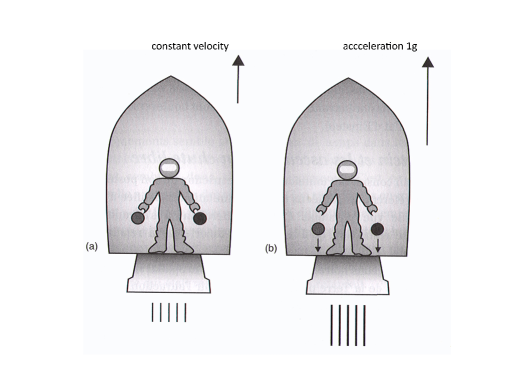
Figure 1: (a) When the astronaut in a rocket in uniform motion (constant velocity) drops the balls, they float around. (b) If the rocket accelerates by $1$ g, the balls fall to the ground and the astronaut has no way to identify whether this due to acceleration or to a gravitational field (i.e. the Earth attraction).

This has several consequences, the most notable of which being that the curves followed by light (null geodesics) are not straight lines (see Fig. 2).

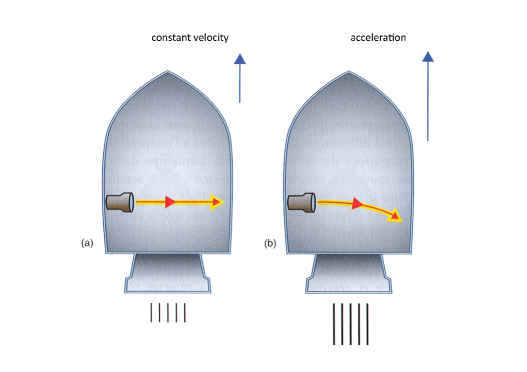
Figure 2: If light propagates along straight lines in the rocket in uniform motion (a), it must deviate from a straight line when the rocket accelerates (b). Thus it must propagate along curved lines in gravitational fields.

Einstein’s equations are highly non-linear second order differential equations for the metric $g_{\mu\nu}$. They read:

$$G_{\mu\nu}\equiv R_{\mu\nu}-{1\over 2}g_{\mu\nu}R=8\pi G_{{}_{N}}T_{\mu\nu}+\lambda g_{\mu\nu}\ .$$ (3)

where $R_{\mu\nu}$ is the Ricci tensor, $R$ the associated curvature scalar (see Appendix .7) and $T_{\mu\nu}$ the energy-momentum tensor; finally $\lambda$ is the cosmological constant which has the dimension of an inverse length squared.

Thus Einstein’s equations relate the geometry of spacetime (the left-hand side of (3)) with its matter field content (the right-hand side).

Einstein equations are field equations. Of which field? This is better understood in the weak gravitational field limit, that is in the limit of an almost flat spacetime. In this case, the metric is approximated by

$$g_{\mu\nu}\sim\eta_{\mu\nu}+h_{\mu\nu}(x)\ ,$$ (4)

where $\eta_{\mu\nu}$ is the Minkowski metric and $h_{\mu\nu}(x)$ is interpreted as the spin-2 graviton field. In particular, we note that

$$g_{00}=1+2\Phi\ ,$$ (5)

where $\Phi$ is the Newtonian potential which satisfies the Poisson equation $\Delta\Phi=4\pi G_{{}_{N}}\rho$.

Einstein used his equations not just to describe a given gravitational system like a planet or a star but the evolution of the whole universe. In his days, this was a bold move: it should be remembered how little of the universe was known at the time these equations were written. “In 1917, the world was supposed to consist of our galaxy and presumably a void beyond. The Andromeda nebula had not yet been certified to lie beyond the Milky Way.”[Pais [Pais] p. 286] Indeed, it is in this context that Einstein introduced the cosmological constant in order to have a static solution (until it was observed by Hubble that the universe is expanding) for the universe.

More precisely [Pais], Einstein first noticed that a slight modification of the Poisson equation, namely

$$\Delta\Phi-\lambda\Phi=4\pi\ G_{{}_{N}}\rho$$ (6)

allowed a solution with a constant density $\rho$ ($\Phi=-4\pi G_{{}_{N}}\rho/\lambda$) and thus a static Newtonian universe. In the context of general relativity, he found a static solution of (3) under the condition that

$$\lambda={1\over r^{2}}=4\pi G_{{}_{N}}\rho\ ,$$ (7)

where $r$ is the spatial curvature (see Exercise 1-1). It was soon shown that this Einstein universe is unstable to small perturbations.

Exercise 1-1 : Consider the following metric

$$g_{00}=1\ ,\quad g_{ij}=-\delta_{ij}+{x_{i}x_{j}\over x^{2}-r^{2}}\ ,\ x^{2}=\sum_{i=1}^{3}x_{i}^{2}\ .$$ (8)

a) Show that it is a solution of Einstein’s equations (3) in the case of non-relativistic matter with a constant energy density $\rho$ satisfying the condition (7).

b) Prove that, in the Newtonian limit, one recovers (6).

Hints: a) $\Gamma^{i}{}_{jk}=r^{-2}\left[x_{i}\delta_{jk}-x_{i}x_{j}x_{k}/(x^{2}-r^{2})\right]$ which gives $R_{ij}=-2g_{ij}/r^{2}$.

b) In the Newtonian limit, $G_{00}\sim\Delta g_{00}$ with $g_{00}$ given by (4).

0.1.2 An expanding Universe

Other solutions to the Einstein equations were soon discovered. The first exact non-trivial one was found in late 1915 by Schwarzschild, who was then fighting in the German army, within a month of the publication of Einstein’s theory and presented on his behalf by Einstein at the Prussian Academy in the first days of 1916 [Sc16], just before Schwarzschild death from a illness contracted at the front. It describes static isotropic regions of empty spacetime ($\lambda=0$), such as the ones encountered in the exterior of a static star of mass $M$ and radius $R$:

$$ds^{2}=\left(1-{2G_{{}_{N}}M\over r}\right)dt^{2}-\left(1-{2G_{{}_{N}}M\over r}\right)^{-1}dr^{2}-r^{2}d\theta^{2}-r^{2}\sin^{2}\theta d\phi^{2}\ .$$ (9)

In 1917, de Sitter proposed a time-dependent vacuum solution in the case where $\lambda\not=0$ [dS17a, dS17b]:

$$ds^{2}=dt^{2}-e^{2Ht}d{\bf x}^{2}\ ,\quad H^{2}\equiv\lambda^{2}/3\ .$$ (10)

But, since there exists time-dependent solutions, why should the Universe be static? This led to the so-called “Great Debate” between Harlow Shapley and Heber D. Curtis in 1920. H. Shapley was supporting the view that the Universe is composed of only one big Galaxy, the spiral nebulae being just nearby gas clouds (he was also arguing –rightfully– that our Sun is far from the center of this big Galaxy). H.D. Curtis, on the other hand considered, that the Universe is made of many galaxies like our own, and that some of these galaxies had already been identified, in the form of the spiral nebulae (and he was supporting the view that our Sun is close to the centre of our relatively small Galaxy).

In 1925, Edwin Hubble studies, with the 100 inch Hooker telescope of Mount Wilson, the Cepheids which are variable stars in the Andromeda nebula M31. He shows that the distance is even greater than the size proposed by Shapley for our Milky Way: M31 is a galaxy of its own, the Andromeda galaxy (at a distance of $3.10^{6}$ light-years from us) [Hu26].

In 1929, Hubble [Hu29] discovers, by combining spectroscopic measurements with measures of distance, that galaxies at a distance $d$ from us recede at a velocity $v$ following the law:

$$v\sim H_{0}d\ ,$$ (11)

the constant of proportionality being henceforth called the Hubble constant (see Fig. 3). As a consequence of the Hubble law, the Universe is expanding!

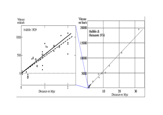
Figure 3: Hubble plot (radial velocity vs distance) of extragalactic “nebulae” obtained by Hubble in his original article of 1929 [Hu29] and by Hubble and Humason two years later [HH31].

The velocities $v$ are measured by Hubble through the Doppler shift of spectroscopic lines of the light emitted by the galaxy: if $\lambda_{{\rm emit}}$ is the wavelength of some spectrocopic line of the light emitted by a galaxy (receding from us at velocity $v$) and $\lambda_{{\rm obs}}$ of the corresponding line in the light observed by us, then

$$1+z\equiv{\lambda_{{\rm obs}}\over\lambda_{{\rm emit}}}={1+v/c\over\sqrt{1-v^{2}/c^{2}}}\sim 1+v/c\ .$$ (12)

Hence $v\sim zc$.

Let us note that stars within galaxies, such are our Sun, are not individually subject to the expansion: they have fallen into the gravitational potential ofthe galaxy and are thus not receding from one another (see Exercise 1-2). This is why one had first to identify extragalactic objects before discovering the expansion: only galaxies, or clusters of galaxies, recede from one another.

Exercise 1-2 : The purpose of this exercise is to show that, in the case where a fluctuation of density appears (such as when galaxies form), the massive objects (stars) decouple from the general expansion to fall into the local gravitational potential [Pe67, We87].

In a matter-dominated universe of uniform density $\rho$, a perturbation appears in the form of a sphere with uniform excess density $\Delta\rho$. Assuming that the gravitational field inside the sphere is described by the Robertson-Walker metric with positive curvature constant $\Delta k>0$, the evolution is governed by the equations

$${{\dot{a}}^{2}\over a^{2}}+{\Delta k\over a^{2}} = {1\over 3}(\rho+\Delta\rho)\ ,$$ (13)

$$a^{3}(\rho+\Delta\rho) = C\ ,$$ (14)

where $C$ is a constant and we neglect the cosmological constant.

a) Show that the solution is given parametrically by

$$a(t) = {C\over 6\Delta k}(1-\cos\eta)\ ,$$ (15)

$$t = t_{0}+{C\over 6\Delta k^{3/2}}(\eta-\sin\eta)\ .$$ (16)

Note that this does not assume that $\Delta\rho$ is small.

b) Show that, as $t\rightarrow t_{0}$, one has $a(t)=(C/3)^{1/3}\left[3(t-t_{0})/2\right]^{2/3}\sim(t-t_{0})^{2/3}$, as in the rest of the matter-dominated universe. Verify that, whereas $\rho=(4/3)(t-t_{0})^{-2}(\sim a^{-3})$, $\Delta\rho=(9/5)\Delta ka^{-2}\sim(t-t_{0})^{-4/3}$.

c) How long does it take before the system starts to collapse to a bound system or to a singularity?

Hints: a) $a{\dot{a}}^{2}+a\Delta k=C/3$

b) Make an expansion in $\eta$ to the subleading order ($\eta$ is small when $t\rightarrow t_{0}$).

c) From (15) the expansion stops and the collapse starts at $\eta=\pi$ or $t-t_{0}=\pi C/(6\Delta k^{3/2})$.

Exercise 1-3 : Identify the redefinition of coordinates $\bar{t}=\bar{t}(t,r)$, $\bar{r}=\bar{r}(t,r)$ which allows to write the de Sitter metric (10)

$$ds^{2}=dt^{2}-e^{2Ht}(dr^{2}+r^{2}d\Omega^{2})\ ,$$ (17)

into the following form:

$$ds^{2}=\left(1-{\bar{r}^{2}\over R_{H}^{2}}\right)d\bar{t}^{2}-\left(1-{\bar{r}^{2}\over R_{H}^{2}}\right)^{-1}d{\bar{r}}^{2}-\bar{r}^{2}d\Omega^{2}\ ,\quad R_{H}\equiv H^{-1}\ .$$ (18)

The first equation is known as the flat form of the de Sitter metric (see (19) below), the second one is the static form (compare with the Schwarzschild metric (9)).

Hints: $e^{Ht}=e^{H\bar{t}}\sqrt{1-H^{2}\bar{r}^{2}}$ and $r=\bar{r}e^{-Ht}$.

0.1.3 Friedmann-Lemaître-Robertson-Walker universe

As one gets to larger and larger distances, the Universe becomes more homogeneous and isotropic. Under the assumption that it reaches homogeneity and isotropy on scales of order $100$ Mpc ($1$ pc $=3.262$ light-year $=3.086\times 10^{16}$ m) and larger, one may first try to find a homogeneous and isotropic metric as a solution of Einstein’s equations. The most general ansatz is, up to coordinate redefinitions, the Robertson-Walker metric:

$$ds^{2} = c^{2}dt^{2}-a^{2}(t)\ \gamma_{ij}dx^{i}dx^{j},$$ (19)

$$\gamma_{ij}dx^{i}dx^{j} = {dr^{2}\over 1-kr^{2}}+r^{2}\left(d\theta^{2}+\sin^{2}\theta d\phi^{2}\right),$$ (20)

where $a(t)$ is the cosmic scale factor, which is time-dependent in an expanding or contracting universe. Such a universe is called a Friedmann-Lemaître universe. The constant $k$ which appears in the spatial metric $\gamma_{ij}$ can take the values $\pm 1$ or $0$: the value $0$ corresponds to flat space, i.e. usual Minkowski spacetime; the value $+1$ to closed space ($r^{2}<1$) and the value $-1$ to open space. Note that $r$ is dimensionless whereas $a$ has the dimension of a length. From now on, we set $c=1$, except otherwise stated.

For the energy-momentum tensor that appears on the right-hand side of Einstein’s equations, we follow our assumption of homogeneity and isotropy and assimilate the content of the Universe to a perfect fluid:

$$T_{\mu\nu}=-pg_{\mu\nu}+(p+\rho)U_{\mu}U_{\nu}\quad,$$ (21)

where $U^{\mu}$ is the velocity 4-vector ($U^{t}=1,U^{i}=0$). It follows from (21) that $T_{tt}=\rho$ and $T_{ij}=a^{2}p\gamma_{ij}$. The pressure $p$ and energy density $\rho$ usually satisfy the equation of state:

$$p=w\rho\quad.$$ (22)

The constant $w$, called the equation of state parameter, takes the value $w\sim 0$ for non-relativistic matter (negligible pressure) and $w=1/3$ for relativistic matter (radiation). In all generality, the perfect fluid consists of several components with different values of $w$.

One obtains from the $(0,0)$ and $(i,j)$ components of the Einstein equations (3) (see Exercise B-1 of Appendix .7):

$$3\left({{\dot{a}}^{2}\over a^{2}}+{k\over a^{2}}\right) = 8\pi G_{{}_{N}}\rho+\lambda,$$ (23)

$${\dot{a}}^{2}+2a{\ddot{a}}+k = -8\pi G_{{}_{N}}a^{2}p+a^{2}\lambda,$$ (24)

where we use standard notations: $\dot{a}$ is the first time derivative of the cosmic scale factor, $\ddot{a}$ the second time derivative.

The first of the preceding equations can be written as the Friedmann equation, which gives an expression for the Hubble parameter $H\equiv\dot{a}/a$ measuring the rate of the expansion of the Universe:

$$H^{2}\equiv{{\dot{a}}^{2}\over a^{2}}={1\over 3}\left(\lambda+8\pi G_{{}_{N}}\rho\right)-{k\over a^{2}}\ .$$ (25)

The cosmological constant appears as a constant contribution to the Hubble parameter. We note that, setting $k=0$ and $\rho=0$, one recovers de Sitter solution (10): $\dot{a}^{2}/a^{2}=\lambda/3$ i.e. $a(t)\sim e^{Ht}$. For the time being, we will set $\lambda$ to zero and return to it in subsequent chapters.

Next, we note that, assuming $k=0$, we have at present time:

$$\rho={3H_{0}^{2}\over 8\pi G_{{}_{N}}}\equiv\rho_{c}\sim 10^{-26}{\rm kg}/{\rm m}^{3}\ ,$$ (26)

where $H_{0}$ is the Hubble constant, i.e. the present value of the Hubble parameter. This corresponds to approximately one galaxy per Mpc³ or $5$ protons per m³. In fundamental units where $\hbar=c=1$, this is of the order of $\left(10^{-3}\hbox{eV}\right)^{4}$. We easily deduce from (25) that space is open (resp. closed) if at present time $\rho<\rho_{c}$ (resp. $\rho<\rho_{c}$). Hence the name critical density for $\rho_{c}$.

Friedmann equation (25) can be understood on very simple grounds: since the universe at large scale is homogeneous and isotropic, there is no specific location and motion in the universe should not allow to identify any such location. This implies that the most general motion has the form ${\bf v}(t)=H(t){\bf x}$ where ${\bf x}$ and ${\bf v}$ denote the position and the velocity and $H(t)$ is an arbitrary function of time. Since ${\bf v}=\dot{\bf x}$, one obtains ${\bf x}=a(t){\bf r}$, where ${\bf r}$ is a constant for a given body (called the comoving coordinate) and $a(t)$ is related to $H(t)$ through $H=\dot{a}/a$. Now, consider a particle of mass $m$ located at position ${\bf x}$: the sum of its kinetic and gravitational potential energy is constant. Denoting by $\rho$ the energy density of the (homogeneous) universe, we have

$${1\over 2}m{\bf v}^{2}-{4\pi\over 3}G_{{}_{N}}m\rho\left|{\bf x}\right|^{2}=\hbox{cst}\ .$$ (27)

Writing this constant $-km{\bf r}^{2}/2$, we obtain from (27)

$${{\dot{a}}^{2}\over a^{2}}={8\pi\over 3}G_{{}_{N}}\rho-{k\over a^{2}}\ ,$$ (28)

which is nothing but Friedmann equation (25) (with vanishing cosmological constant).

Friedmann equation should be supplemented by the conservation of the energy-momentum tensor which simply yields:

$$\dot{\rho}=-3H(p+\rho)\quad.$$ (29)

Hence a component with equation of state (22) has its energy density scaling as $\rho\sim a(t)^{-3(1+w)}$. Thus non-relativistic matter (often referred to as matter) energy density scales as $a^{-3}$. In other words, the energy density of matter evolves in such a way that $\rho a^{3}$ remains constant. Radiation scales as $a^{-4}$ and a component with equation of state $p=-\rho$ ($w=-1$) has constant energy density.

We note for future use that, if a component with equation of state (22) dominates the energy density of the universe (as well as the curvature term $-k/a^{2}$), then (28) has a scaling solution

$$a(t)\sim t^{\nu}\ ,\quad\hbox{with}\ \nu={2\over 3(1+w)}\ .$$ (30)

For example, in a matter-dominated universe, $a(t)\sim t^{2/3}$, and in a radiation-dominated universe, $a(t)\sim t^{1/2}$.

Differentiating the Friedmann equation with respect to time, and using the energy-momentum conservation (29), one easily obtains

$$\ddot{a}=-{4\pi G_{{}_{N}}\over 3}a(3p+\rho)+a{\lambda\over 3}\ .$$ (31)

This allows to recover (24) from Friedmann equation and energy-momentum conservation.

0.1.4 Redshift

In an expanding or contracting universe, the Doppler frequency shift undergone by the light emitted from a distant source gives a direct information on the time dependence of the cosmic scale factor $a(t)$. To obtain the explicit relation, we consider a photon propagating in a fixed direction ($\theta$ and $\phi$ fixed). Its equation of motion is given as in special relativity by setting $ds^{2}=0$ in (19):

$$c^{2}dt^{2}=a^{2}(t){dr^{2}\over 1-kr^{2}}\quad.$$ (32)

Thus, if a photon (an electromagnetic wave) leaves at time $t$ a galaxy located at distance $r$ from us, it will reach us at time $t_{0}$ such that

$$\int_{t}^{t_{0}}{cdt\over a(t)}=\int_{0}^{r}{dr\over\sqrt{1-kr^{2}}}$$ (33)

The electromagnetic wave is emitted with the same amplitude at a time $t+T$ where the period $T$ is related to the wavelength of the emitted wave $\lambda$ by the relation $\lambda=cT$. It is thus received with the same amplitude at the time $t_{0}+T_{0}$ given by

$$\int_{t+T}^{t_{0}+T_{0}}{cdt\over a(t)}=\int_{0}^{r}{dr\over\sqrt{1-kr^{2}}}\quad,$$ (34)

the wavelength of the received wave being simply $\lambda_{0}=cT_{0}$. Since $T_{0},T\ll t_{0},t$, we obtain from comparing (33) and (34)

$${cT_{0}\over a_{0}}={cT\over a(t)}\qquad\hbox{i.e.}\qquad{\lambda_{0}\over\lambda}={a_{0}\over a(t)}\quad,$$ (35)

where $a_{0}$ is the present value of the cosmic scale factor.

Defining the redshift parameter $z$ as the fractional increase in wavelength $z=(\lambda_{0}-\lambda)/\lambda$, we have

$$1+z={a_{0}\over a(t)}\quad.$$ (36)

One may thus replace time by redshift since time decreases monotonically as redshift increases.

0.1.5 The universe today: energy budget

The Friedmann equation

$$H^{2}\equiv{{\dot{a}}^{2}\over a^{2}}={1\over 3}\left(\lambda+8\pi G_{{}_{N}}\rho\right)-{k\over a^{2}}\ .$$ (37)

allows to define the Hubble constant $H_{0}$, i.e. the present value of the Hubble parameter, which sets the scale of our Universe at present time. Because of the troubled history of the measurement of the Hubble constant, it has become customary to express it in units of $100\ \hbox{km}.\hbox{s}^{-1}.\hbox{Mpc}^{-1}$ which gives its order of magnitude. Present measurements give

$$h_{0}\equiv{H_{0}\over 100\ \hbox{km}.\hbox{s}^{-1}.\hbox{Mpc}^{-1}}=0.7\pm 0.1\quad.$$

The corresponding length and time scales are:

$$\ell_{H_{0}} \equiv {c\over H_{0}}=3000\ h_{0}^{-1}\ \hbox{Mpc}=9.25\times 10^{25}\ h_{0}^{-1}\ \hbox{m},$$ (38)

$$t_{H_{0}} \equiv {1\over H_{0}}=3.1\times 10^{17}\ h_{0}^{-1}\ \hbox{s}=9.8\ h_{0}^{-1}\ \hbox{Gyr}.$$ (39)

It has become customary to normalize the different forms of energy density in the present Universe in terms of the critical density $\rho_{c}=3H_{0}^{2}/(8\pi G_{{}_{N}})$ defined in (26). Separating the energy density $\rho_{{}_{M0}}$ presently stored in non-relativistic matter (baryons, neutrinos, dark matter,…) from the density $\rho_{{}_{R0}}$ presently stored in radiation (photons, relativistic neutrino if any), one defines:

$$\Omega_{{}_{M}}\equiv{\rho_{{}_{M0}}\over\rho_{c}},\;\;\;\;\Omega_{{}_{R}}\equiv{\rho_{{}_{R0}}\over\rho_{c}},\;\;\;\;\Omega_{\Lambda}\equiv{\lambda\over 3H_{0}^{2}},\;\;\Omega_{k}\equiv-{k\over a_{0}^{2}H_{0}^{2}}\ .$$ (40)

The last term comes from the spatial curvature and is not strictly speaking a contribution to the energy density. One may add other components: we will refrain to do so in this Chapter and defer this to the last one.

Then the Friedmann equation taken at time $t_{0}$ simply reads

$$\Omega_{{}_{M}}+\Omega_{{}_{R}}+\Omega_{\Lambda}=1-\Omega_{k}\ .$$ (41)

Since matter dominates over radiation in the present Universe, we may neglect $\Omega_{{}_{R}}$ in the preceding equation. As we will see in the next Chapters, present observational data tend to favor the following set of values: $\Omega_{k}\sim 0$ (see Section 0.2.1) and $\Omega_{{}_{M}}\sim 0.3$, $\Omega_{\Lambda}\sim 0.7$ (see Section 0.5.1 and Fig. 22). The matter density is not consistent with the observed density of luminous matter ($\Omega_{{\rm luminous}}\sim 0.04$) and thus calls for a nonluminous form of matter, dark matter which will be studied in Section 0.4.

Using the dependence of the different components with the scale factor $a(t)=a_{0}/(1+z)$, one may then rewrite the Friedmann equation at any time as:

$$H^{2}(t) = H_{0}^{2}\left[\Omega_{\Lambda}+\Omega_{{}_{M}}\left({a_{0}\over a(t)}\right)^{3}+\Omega_{{}_{R}}\left({a_{0}\over a(t)}\right)^{4}+\Omega_{k}\left({a_{0}\over a(t)}\right)^{2}\right]\ ,$$ (42)

$$\hbox{or}\ H^{2}(z) = H_{0}^{2}\left[\Omega_{{}_{M}}(1+z)^{3}+\Omega_{{}_{R}}(1+z)^{4}+\Omega_{k}(1+z)^{2}+\Omega_{\Lambda}\right]\ .$$ (43)

where $a_{0}$ is the present value of the cosmic scale factor and all time dependences (or alternatively redshift dependence) have been written explicitly. We note that, even if $\Omega_{{}_{R}}$ is negligible in (41), this is not so in the early Universe because the radiation term increases faster than the matter term in (42) as one gets back in time (i.e. as $a(t)$ decreases). If we add an extra component $X$ with equation of state $p_{{}_{X}}=w_{{}_{X}}\rho_{{}_{X}}$, it contributes an extra term $\Omega_{{}_{X}}\left(a_{0}/a(t)\right)^{3(1+w_{{}_{X}})}$ where $\Omega_{{}_{X}}=\rho_{{}_{X}}/\rho_{c}$.

An important information about the evolution of the universe at a given time is whether its expansion is accelerating or decelerating. The acceleration of our universe is usually measured by the deceleration parameter $q$ which is defined as:

$$q\equiv-{\ddot{a}a\over\dot{a}^{2}}\quad.$$ (44)

Using (31) of Section 0.2 and separating again matter and radiation, we may write it at present time $t_{0}$ as:

$$q_{0}=-{1\over H_{0}^{2}}\left({\ddot{a}\over a}\right)_{t=t_{0}}={1\over 2}\Omega_{{}_{M}}+\Omega_{{}_{R}}-\Omega_{\Lambda}\quad.$$ (45)

Once again, the radiation term $\Omega_{{}_{R}}$ can be neglected in this relation. We see that in order to have an acceleration of the expansion ($q_{0}<0$), we need the cosmological constant to dominate over the other terms.

We can also write the deceleration parameter in (44) in terms of redshift as in (43)

$$q={H_{0}^{2}\over 2H(z)^{2}}\left[\Omega_{{}_{M}}(1+z)^{3}+2\Omega_{{}_{R}}(1+z)^{4}-2\Omega_{\Lambda}\right]\quad.$$ (46)

This shows that the universe starts accelerating at redshift values $1+z\sim\left(2\Omega_{\Lambda}/\Omega_{{}_{M}}\right)^{1/3}$ (neglecting $\Omega_{{}_{R}}$), that is typically redshifts of order $1$.

The measurements of the Hubble constant and of the deceleration parameter at present time allow to obtain the behaviour of the cosmic scale factor in the last stages of the evolution of the universe:

$$a(t)=a_{0}\left[1+{t-t_{0}\over t_{H_{0}}}-{q_{0}\over 2}{(t-t_{0})^{2}\over t_{H_{0}}^{2}}+\cdots\right]\ .$$ (47)

0.1.6 The early universe

Table 1 summarizes the history of the universe in the context of the big bang model with an inflationary epoch. We are referring to the different stages using time, redshift or temperature. The last two can be related using the conservation of entropy.

Indeed, one can show, using the second law of thermodynamics ($TdS=dE+pdV$) that the entropy per unit volume is simply the quantity

$$s\equiv{S\over V}={\rho+p\over T}$$ (48)

and that the entropy in a covolume $sa^{3}$ remains constant. The entropy density is dominated by relativistic particles and reads

$$s = {2\over 3}g_{s}(T)a_{{}_{BB}}T^{3}\quad,$$ (49)

$$g_{s}(T) = \sum_{{\rm bosons}\ i}g_{i}\left({T_{i}\over T}\right)^{3}+{7\over 8}\sum_{{\rm fermions}\ i}g_{i}\left({T_{i}\over T}\right)^{3}\quad,$$ (50)

where the sum extends only to the species in thermal equilibrium and $a_{{}_{BB}}\equiv\pi^{2}k^{4}/(15c^{3}\hbar^{3})=7.56\times 10^{-16}\ {\rm J}\cdot{\rm m}^{-3}\cdot{\rm K}^{-4}$ is the blackbody constant.

We deduce from the constancy of $sa^{3}$ that $g_{s}\left(aT\right)^{3}$ remains constant. Hence the temperature $T$ of the universe behaves as $a^{-1}$ whenever $g_{s}$ remains constant. We conclude that as we go back in time ($a$ decreases), temperature increases, as well as energy density. The early universe is hot and dense. It might even reach a stage where our equations no longer apply because it becomes infinitely hot and dense: this is the initial singularity, sarcastically (but successfully) called big bang by Fred Hoyle, on a BBC radio show in 1949.

We note that some caution has to be paid whenever some species drop out of thermal equilibrium. Indeed, a given species drops out of equilibrium when its interaction rate $\Gamma$ drops below the expansion rate $H$. For example neutrinos decouple at temperatures below 1 MeV. Their temperature continues to decrease as $a^{-1}$ and thus remains equal to $T$. However when $kT$ drops below $2m_{e}$, electrons annihilate against positrons with no possibility of being regenerated and the entropy of the electron-positron pairs is transferred to the photons. Since $\left.g_{s}\right|_{\gamma,e^{\pm}}=2+4\cdot 7/8=11/2$ and $\left.g_{s}\right|_{\gamma}=2$, the temperature of the photons becomes multiplied by a factor $(11/4)^{1/3}$. Since the neutrinos have already decoupled, they are not affected by this entropy release and their temperature remains untouched. Thus we have

$${T\over T_{\nu}}=\left({11\over 4}\right)^{1/3}\sim 1.40\quad.$$ (51)

We can then compute the value of $g_{s}$ for temperatures much smaller than $m_{e}$: $g_{s}=2+(7/8)6(4/11)=3.91$. We deduce that, at present time ($T_{0}=2.725$ K), $s_{0}/k=2890\ {\rm cm}^{-3}$.

Table 1: The different stages of the cosmological evolution in the standard scenario, given in terms of time $t$ since the big bang singularity, the energy $kT$ of the background photons and the redshift $z$. The double line following nucleosynthesis indicates the part of the evolution which has been tested through observation. The values $(h_{0}=0.7,\Omega_{{}_{M}}=0.3,\Omega_{\Lambda}=0.7)$ are adopted to compute explicit values.

$t$	$kT_{\gamma}$ (eV)	$z$
$t_{0}\sim 15$ Gyr	$2.35\times 10^{-4}$	$0$	now
$\sim$ Gyr	$\sim 10^{-3}$	$\sim 10$	formation of galaxies
$t_{{}_{\rm rec}}\sim 4\times 10^{5}$ yr	$0.26$	$1100$	recombination
$t_{{}_{\rm eq}}\sim 4\times 10^{4}$ yr	$0.83$	$3500$	matter-radiation equality
$3$ min	$6\times 10^{4}$	$2\times 10^{8}$	nucleosynthesis
$1$ s	$10^{6}$	$3\times 10^{9}$	$e^{+}e^{-}$ annihilation
$4\times 10^{-6}$ s	$4\times 10^{8}$	$10^{12}$	QCD phase transition
$<4\times 10^{-6}$ s	$>10^{9}$		baryogenesis
			inflation
$t=0$		$\infty$	big-bang

As we have seen in (30), it follows from the Friedmann equation that, if the Universe is dominated by a component of equation of state $p=w\rho$, then the cosmic scale factor $a(t)$ varies with time as $t^{2/[3(1+w)]}$. We start at time $t_{0}$ with the energy budget: $\Omega_{{}_{M}}=0.3,\Omega_{\Lambda}=0.7,\Omega_{k}\sim 0$ (see next Chapters). Radiation consists of photons and relativistic neutrinos. Since generically

$$\rho_{{}_{R}}={1\over 2}g(T)a_{{}_{BB}}T^{4}\ ,$$ (52)

where $g(T)$ is the effective number of degrees of freedom

$$g(T)=\sum_{{\rm bosons}\ i}g_{i}\left({T_{i}\over T}\right)^{4}+{7\over 8}\sum_{{\rm fermions}\ i}g_{i}\left({T_{i}\over T}\right)^{4}$$ (53)

(we have taken into account the possibility that the species $i$ may have a thermal distribution at a temperature $T_{i}$ different from the temperature $T$ of the photons), we have

$$\rho_{{}_{R}}(t)=\rho_{\gamma}(t)\left[1+{7\over 8}\left({4\over 11}\right)^{4/3}\ N_{\nu}^{{\rm rel}}(t)\right]\quad,$$ (54)

where $N_{\nu}^{{\rm rel}}(t)$ is the number of relativistic neutrinos at time $t$. At present time $t_{0}$, we have $\Omega_{\gamma}=\rho_{\gamma}(t_{0})/\rho_{c}=2.48\times 10^{-5}\ h^{-2}$ and the mass limits on neutrinos imply $N_{\nu}^{{\rm rel}}(t_{0})\leq 1$. In any case, $\Omega_{{}_{R}}\ll\Omega_{{}_{M}}$.

For redshifts larger than 1, the cosmological constant becomes subdominant and the universe is matter-dominated ($a(t)\sim t^{2/3}$). In the early phase of this matter-dominated epoch, the Universe is a ionized plasma with electrons and protons: it is opaque to photons. But, at a time $t_{{}_{{\rm rec}}}$, electrons recombine with the protons to form atoms of hydrogen and, because hydrogen is neutral, this induces the decoupling of matter and photon: from then on ($t_{{}_{{\rm rec}}}<t<t_{0}$), the universe is transparent. This is the important recombination stage. After decoupling the energy density $\rho_{\gamma}\sim T^{4}$ of the primordial photons is redshifted according to the law

$${T(t)\over T_{0}}={a_{0}\over a(t)}=1+z\quad.$$ (55)

One observes presently this cosmic microwave background (CMB) as a radiation with a black-body spectrum at temperature $T_{0}=2.725$ K or energy $kT_{0}=2.35\times 10^{-4}$ eV.

Since the binding energy of the ground state of atomic hydrogen is $E_{b}=13.6$ eV, one may expect that the energy $kT_{{}_{{\rm rec}}}$ is of the same order. It is substantially smaller because of the smallness of the ratio of baryons to photons $\eta=n_{b}/n_{\gamma}\sim 5\times 10^{-10}$. Indeed, according to the Saha equation, the fraction $x$ of ionized atoms is given by

$${n_{p}n_{e}\over n_{H}n_{\gamma}}={x^{2}\over(1-x)}\eta={4.05c^{3}\over\pi^{2}}\left({m_{e}\over 2\pi kT}\right)^{3/2}e^{-E_{b}/kT}\quad.$$ (56)

Hence, because $\eta\ll 1$, the ionized fraction $x$ becomes negligible only for energies much smaller than $E_{b}$. A careful treatment gives $kT_{{}_{{\rm rec}}}\sim 0.26$ eV.

As we proceed back in time, radiation energy density increases more rapidly (as $a(t)^{-4}$) than matter ($a(t)^{-3}$) (as $a(t)$ decreases). At time $t_{{\rm eq}}$, there is equality. This corresponds to

$${1\over 1+z_{{\rm eq}}}={a(t_{{\rm eq}})\over a_{0}}={1.68\ \Omega_{\gamma}\over\Omega_{{}_{M}}}={4.17\times 10^{-5}\over\Omega_{{}_{M}}h_{0}^{2}}\quad,$$ (57)

where we have assumed 3 relativistic neutrinos at this time.

As we go further back in time, we presumably reach a period where matter overcame antimatter. It is indeed a great puzzle of our Universe to observe so little antimatter, when our microscopic theories treat matter and antimatter on equal footing. More quantitatively, one has to explain the following very small number:

$$\eta\equiv{n_{B}\over n_{\gamma}}={n_{b}-n_{\bar{b}}\over n_{\gamma}}\sim 6\times 10^{-10}\ ,$$ (58)

where $n_{B}=n_{b}-n_{\bar{b}}$ (resp. $n_{\gamma}$) is the baryon (resp. photon) number density, based on baryon $b$ and antibaryon $\bar{b}$ counts. The actual number comes from the latest Planck data [Planck13_16].

Sakharov [Sa67] gave in 1967 the necessary ingredients to generate an asymmetry between matter and antimatter:

• a process that destroys baryon number,

• a violation of the symmetry between matter and antimatter (the so-called charge conjugation), as well as a violation of the time reversal symmetry,

• an absence of thermal equilibrium.

The Standard Model ensures the second set of conditions (CP violation which was discovered by Cronin and Fitch [CF64] is accounted for by the phase of the CKM matrix). The expanding early universe provides the third condition. It remains to find a process that destroys baryon number. Different roads were followed: non-perturbative processes (sphaleron) at the electroweak phase transition; proton decay in the context of grand unified theories; decay of heavy neutrinos which leads to lepton number violation, and consequently to baryon number violation (leptogenesis).

0.2 The days where cosmology became a quantitative science: cosmic microwave background

We have recalled briefly in Section 0.1.6 the history of the Universe (see Table 1). The very early universe is a ionized plasma, and thus is opaque to light. But we have seen that, soon after matter-radiation equality, electrons recombined with the protons to form neutral atoms of hydrogen, which induces the decoupling of matter and photon. From this epoch on, the universe becomes transparent to light. The primordial gas of photons produced at this epoch cools down as the universe expands (following 55) and forms nowadays the cosmic microwave background (CMB).

Bell Labs radio astronomers Arno Penzias and Robert Wilson were using a large horn antenna in 1964 and 1965 to map signals from the Milky Way, when they accidently discovered the CMB [PW65]. The discovery of this radiation was a major confirmation of the hot big bang model: its homogeneity and isotropy was a signature of its cosmological origin. However, the degree of homogeneity and isotropy of this radiation was difficult to reconcile with the history of the Universe as understood from the standard big bang theory: radiation coming from regions of the sky which were not supposed to be causally connected in the past had exactly the same properties.

It was for such reasons that the scenario of inflation was proposed [St80, Gu81]: an exponential expansion of the Universe right after the big bang. In the solution proposed by A. Guth [Gu81], the set up was the spontaneous breaking of the grand unified theory: the corresponding phase transition was providing the vacuum energy necessary to initiate such an exponential expansion. This scenario proved to be difficult to realize and it was followed by many variants: new inflation [Li82], chaotic inflation [Li83], …

We have said that, for $t<t_{{}_{{\rm rec}}}$, i.e. $z>1100$, the Universe is a ionized plasma, opaque to electromagnetic radiation. This means that, when we observe the early Universe, we hit a “wall” at the corresponding redshift: the earlier Universe appears to our observation as a blackbody, and should thus radiate according to the predictions of Planck. This is certainly the largest blackbody that one could think of. This blackbody spectrum of the CMB was indeed observed [MA90] by the FIRAS instrument onboard the COsmic Background Explorer (COBE) satellite launched in 1989 by NASA (see Fig. 4).

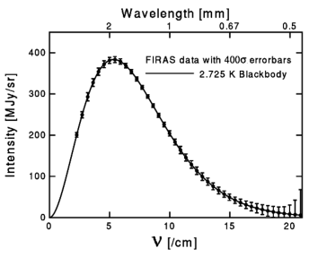
Figure 4: Blackbody spectrum of the CMB as observed by the instrument FIRAS onboard the COBE satellite [MA90]

More precisely, the CMB has the nearly perfect thermal spectrum of a black body at temperature $T_{\gamma}=2.725$ K (corresponding to a number density $n_{\gamma}=411$ cm^-3):

$$d\rho_{\gamma}=2hf{1\over e^{hf/kT_{\gamma}}-1}{4\pi f^{2}df\over c^{3}}$$ (59)

(the first factor accounts for the two polarizations) or

$${d\rho_{\gamma}\over d\ln f}=3.8\times 10^{-15}\hbox{J/m}^{3}\left({f\over f_{\gamma}}\right)^{4}{e-1\over e^{f/f_{\gamma}}-1}\ ,$$ (60)

where $f_{\gamma}=kT_{\gamma}/h=5.7\times 10^{10}$ Hz.

Another expectation for COBE was the presence of fluctuations in the CMB. Indeed, if inflation was to explain the puzzle of isotropy and homogeneity of the CMB through the whole sky, one expected that quantum fluctuations produced during the inflation phase would show up to some degree as tiny fluctuations of temperature in the CMB. Such fluctuations were discovered by the instrument DMR (Differential Microwave Radiometers) onboard COBE, at the level of one part to $10^{5}$ [Sm92] (see Fig. 5).

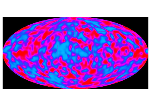
Figure 5: Temperature fluctuations in the CMB observed by COBE [Sm92] (the galaxy is removed). The galaxy as well as the dipole component associated to the Doppler effect due to the motion of the Earth have been removed. Blue areas are colder than average, red areas are warmer but no $7^{\circ}$ region varies from the mean by more than $200$ $\mu$K ($\Delta T/T\sim 8.10^{-5}$).

It is primarily homogeneous and isotropic but includes fluctuations at a level of $10^{-5}$, which are of much interest since they are .

Since the days of COBE, there has been an extensive study of the CMB fluctuations to identify the imprints of the recombination and earlier epochs. This uses the results of ground, balloon or space missions (WMAP in the US and most recently Planck in Europe). We will review this in some details in the next Section.

0.2.1 CMB

Before discussing the spectrum of CMB fluctuations, we introduce the important notion of a particle horizon in cosmology.

Because of the speed of light, a photon which is emitted at the big bang ($t=0$) will have travelled a finite distance at time $t$. The proper distance (248) measured at time $t$ is simply given by the integral:

$$d_{ph}(t) = a(t)\int_{0}^{t}{cdt^{\prime}\over a(t^{\prime})}$$

$$= {\ell_{H_{0}}\over 1+z}\int_{z}^{\infty}{dz\over\left[\Omega_{{}_{M}}(1+z)^{3}+\Omega_{{}_{R}}(1+z)^{4}+\Omega_{k}(1+z)^{2}+\Omega_{\Lambda}\right]^{1/2}}\quad,$$

where, in the second line, we have used (.8). This is the maximal distance that a photon (or any particle) could have travelled at time $t$ since the big bang. In other words, it is possible to receive signals at a time $t$ only from comoving particles within a sphere of radius $d_{h}(t)$. This distance is known as the particle horizon at time $t$.

A quantity of relevance for our discussion of CMB fluctuations is the horizon at the time of the recombination i.e. $z_{{}_{{\rm rec}}}\sim 1100$. We note that the integral on the second line of (0.2.1) is dominated by the lowest values of $z$: $z\sim z_{{}_{{\rm rec}}}$ where the universe is still matter dominated. Hence

$$d_{ph}(t_{{}_{{\rm rec}}})\sim{2\ell_{H_{0}}\over\Omega_{{}_{M}}^{1/2}z_{{}_{{\rm rec}}}^{3/2}}\sim 0.3\ \hbox{Mpc}\ .$$ (62)

One may introduce also the Hubble radius

$$R_{H}(t)=H^{-1}(z)\ ,$$ (63)

which will play an important role in the following discussion. This scale characterizes the curvature of spacetime at the time $t$ (see for example Exercise B.1.b). We note that the particle horizon is simply twice the Hubble radius at recombination, as can be checked from (43):

$$R_{H}(t_{{}_{{\rm rec}}})\sim{\ell_{H_{0}}\over\Omega_{{}_{M}}^{1/2}z_{{}_{{\rm rec}}}^{3/2}}\ .$$ (64)

This radius is seen from an observer at present time under an angle

$$\theta_{H}(t_{{}_{{\rm rec}}})={R_{H}(t_{{}_{{\rm rec}}})\over d_{A}(t_{{}_{{\rm rec}}})}\ ,$$ (65)

where the angular distance has been defined in (257). We can compute analytically this angular distance under the assumption that the universe is matter dominated (see Exercise C-1). Using (260), we have

$$d_{A}(t_{{}_{{\rm rec}}})={a_{0}r\over 1+z_{{}_{{\rm rec}}}}\sim{2\ell_{H_{0}}\over\Omega_{{}_{M}}z_{{}_{{\rm rec}}}}\ .$$ (66)

Thus, since, in our approximation, the total energy density $\Omega_{{}_{T}}$ is given by $\Omega_{{}_{M}}$,

$$\theta_{H}(t_{{}_{{\rm rec}}})\sim\Omega_{{}_{T}}^{1/2}/(2z_{{}_{{\rm rec}}}^{1/2})\sim 0.015\ \hbox{rad}\ \Omega_{{}_{T}}^{1/2}\sim 1^{\circ}\ \Omega_{{}_{T}}^{1/2}\ .$$ (67)

We have written in the latter equation $\Omega_{{}_{T}}$ instead of $\Omega_{{}_{M}}$ because numerical computations show that, in case where $\Omega_{\Lambda}$ is non-negligible, the angle depends on $\Omega_{{}_{M}}+\Omega_{\Lambda}=\Omega_{{}_{T}}$.

We can now discuss the evolution of photon temperature fluctuations. For simplicity, we will assume a flat primordial spectrum of fluctuations: this leads to predictions in good agreement with experiment; moreover, as we will see in the next Section, it is naturally explained in the context of inflation scenarios.

Before decoupling, the photons are tightly coupled with the baryons through Thomson scattering. In a gravitational potential well, gravity tends to pull this baryon-photon fluid down the well whereas radiation pressure tends to push it out. Thus, the fluid undergoes a series of acoustic oscillations. These oscillations can obviously only proceed if they are compatible with causality i.e. if the corresponding wavelength is smaller than the horizon scale or the Hubble radius: $\lambda=2\pi a(t)/k<R_{H}(t)$ or

$$k>2\pi{a(t)\over R_{H}(t)}\sim t^{-1/3}\ .$$ (68)

Figure 6: Evolution of the photon temperature fluctuations before the recombination. This diagram illustrates that oscillations start once the corresponding Fourier mode enters the Hubble radius (these oscillations are fluctuations in temperature, along a vertical axis orthogonal to the two axes that are drawn on the figure).

Starting with a flat primordial spectrum, we see that the first oscillation peak corresponds to $\lambda\sim R_{H}(t_{{}_{{\rm rec}}})$, followed by other compression peaks at $R_{H}(t_{{}_{{\rm rec}}})/n$ (see Fig. 6). They correspond to an angular scale on the sky:

$$\theta_{n}\sim{R_{H}(t_{{}_{{\rm rec}}})\over d_{A}(t_{{}_{{\rm rec}}})}{1\over n}={\theta_{H}(t_{{}_{{\rm rec}}})\over n}\ .$$ (69)

Since photons decouple at $t_{{}_{{\rm rec}}}$, we observe the same spectrum presently (up to a redshift in the photon temperature).

Experiments usually measure the temperature difference of photons received by two antennas separated by an angle $\theta$, averaged over a large fraction of the sky. Defining the correlation function

$$C(\theta)=\left\langle{\Delta T\over T_{0}}({\bf n}_{1}){\Delta T\over T_{0}}({\bf n}_{2})\right\rangle$$ (70)

averaged over all ${\bf n}_{1}$ and ${\bf n}_{2}$ satisfying the condition ${\bf n}_{1}\cdot{\bf n}_{2}=\cos\theta$, we have indeed

$$\left\langle\left({T({\bf n}_{1})-T({\bf n}_{2})\over T_{0}}\right)^{2}\right\rangle=2\left(C(0)-C(\theta)\right).$$ (71)

We may decompose $C(\theta)$ over Legendre polynomials:

$$C(\theta)={1\over 4\pi}\sum_{l}^{\infty}(2l+1)C_{l}P_{l}(\cos\theta)\ .$$ (72)

The monopole ($l=0$), related to the overall temperature $T_{0}$, and the dipole ($l=1$), due to the Solar system peculiar velocity, bring no information on the primordial fluctuations. A given coefficient $C_{l}$ characterizes the contribution of the multipole component $l$ to the correlation function. If $\theta\ll 1$, the main contribution to $C_{l}$ corresponds to an angular scale $\theta\sim\pi/l\sim 200^{\circ}/l$. The previous discussion (see (67) and (69)) implies that we expect the first acoustic peak at a value $l\sim 200\Omega_{{}_{T}}^{-1/2}$.

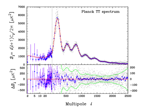
Figure 7: This figure compares the temperature spectrum for the best fit $\Lambda$CDM model, in red, with the temperature angular power spectrum observed by the Planck collaboration (in blue, averaged over bins of width $\Delta l\sim 31$ with 1 $\sigma$ errors). The gray dots are the unbinned data. In the lower panel, the green lines show the $\pm 1\sigma$ errors on the individual power spectrum estimates.[Planck13_16]

The power spectrum obtained by the Planck experiment is shown in Fig. 7. One finds the first acoustic peak at $l\sim 200$, which constrains the $\Lambda$CDM model used to perform the fit to $\Omega_{{}_{T}}=\Omega_{{}_{M}}+\Omega_{\Lambda}\sim 1$. Many other constraints may be inferred from a detailed study of the power spectrum [WMAP03, Planck13_16].

0.2.2 Baryon acoustic oscillations

We noted in the previous section that, before decoupling, baryons and photons were tightly coupled and the baryon-photon fluid underwent a series of acoustic oscillations, which have left imprints in the CMB: the characteristic distance scale is the sound horizon, which is the comoving distance that sound waves could travel from the Big Bang until recombination at $z=z_{*}$:

$$r_{s}=\int_{0}^{t_{*}}{c_{s}(t)\over 1+z}dt=\int_{z_{*}}^{\infty}{c_{s}(z)\over H(z)}dz\ ,$$ (73)

where $c_{s}$ is the sound velocity. This distance has been recently measured with precision by the Planck collaboration to be $r_{s}=144.96\pm 0.66$ Mpc [Planck13_16].

We have until now followed the fate of photons after decoupling. Similarly, once baryons decouple from the radiation, their oscillations freeze in, which leads to specific imprints in the galaxy power spectrum, such as the characteristic scale $r_{s}$. Indeed, remember that, until recombination, baryons and photons were tightly coupled (but not dark matter). Thus a given matter density perturbation may have travelled a distance $r_{s}$ in the case of baryons under the influence of radiation pressure (to which the photons are sensitive), whereas it did not move in the case of dark matter. This will lead, once (dark and baryonic) matter has collapsed into galaxies, to a secondary peak a distance $r_{s}$ away in the distribution of separations of pairs of galaxies. In 2005, Eisenstein and collaborators [Ei05], using data from the Sloan Digital Sky Survey, have indeed identified such a baryon acoustic peak in the matter power spectrum (Fourier transform of the two-point correlation function) on scales of order $105h^{-1}\sim 150$ Mpc. Figure 41 shows how the $\Lambda$CDM model just described fares with respect to observations by comparison with a model with $\Omega_{\Lambda}=0$, a small value of the Hubble parameter and a small fraction of matter which does not cluster on small scale (relic neutrinos or quintessence).

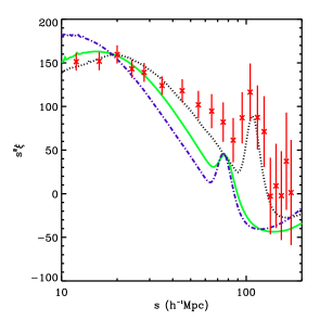
Figure 8: Correlation function in redshift space for the best-fit power-law $\Lambda$CDM model (dotted line) and for the best-fit model with $\Omega_{\Lambda}=0,H_{0}=46$ km/s/Mpc and a relic neutrino component $\Omega_{\nu}=0.12$ (solid line) or a quintessence component $\Omega_{Q}=0.12$ (dot-dashed line) [BDRS06].

The acoustic peak provides a standard ruler which can be used for measuring distances: measurements along the line of sight depend on $H(z)r_{s}$ whereas measurements transverse to the line of sight depend on the angular diameter distance $d_{A}(z)/r_{s}$. In fact, because the analysis rests on spherically-averaged two-point statistics, the distance scale determined is $d_{V}$ defined as:

$$\left({d_{V}(z)\over r_{s}}\right)^{3}\equiv\left({d_{A}(z)\over r_{s}}\right)^{2}{cz\over H(z)r_{s}}\ .$$ (74)

Measuring the acoustic scale at $z=0$ provides a standard distance ruler which allows to identify $H_{0}$, and then $\Omega_{{}_{M}}$ (from $\Omega_{{}_{M}}h^{2}$). Going to higher $z$, this allows to put constraints on the recent history of the Universe, and thus on the evolution of the dark matter component.

0.2.3 Inflation

The inflation scenario has been proposed to solve a certain number of problems faced by the cosmology of the early universe [Gu81]. Among these one may cite:

• the flatness problem

  If the total energy density $\rho_{T}$ of the universe is presently close to the critical density, it should have been even more so in the primordial universe. Indeed, we can write (25) of Section 0.2 as

  $${\rho_{T}(t)\over\rho_{c}(t)}-1={k\over\dot{a}^{2}}\quad,$$ (75)

  where $\rho_{c}(t)=3H^{2}(t)/(8\pi G_{{}_{N}})$ and the total energy density $\rho_{T}$ includes the vacuum energy. If we take for example the radiation-dominated era where $a(t)\sim t^{1/2}$, then (75) can be written as ($\dot{a}\sim t^{-1/2}\sim a^{-1}$)

  $${\rho_{T}(t)\over\rho_{c}(t)}-1=\left[{\rho_{T}(t_{{}_{U}})\over\rho_{c}(t_{{}_{U}})}-1\right]\left({a(t)\over a(t_{{}_{U}})}\right)^{2}=\left[{\rho_{T}(t_{{}_{U}})\over\rho_{c}(t_{{}_{U}})}-1\right]\left({kT_{{}_{U}}\over kT}\right)^{2}\quad,$$ (76)

  where we have used the fact that $T(t)\propto a(t)^{-1}$ and we have taken as a reference point the epoch $t_{{}_{U}}$ of the grand unification phase transition. This means that, if the total energy density is close to the critical density at matter-radiation equality (as can be inferred from the present value), it must be even more so at the time of the grand unification phase transition: by a factor $\left(1\hbox{eV}/10^{16}\hbox{GeV}\right)^{2}\sim 10^{-50}$! Obviously, the choice $k=0$ in the spatial metric ensures $\rho_{{}_{T}}=\rho_{c}$ but the previous estimate shows that this corresponds to intial conditions which are highly fine tuned.

• the horizon problem

  We have stressed in the previous Sections the isotropy and homogeneity of the cosmic microwave background and identified its primordial origin. It remains that the horizon at recombination is seen on the present sky under an angle of $2^{\circ}$. This means that two points opposite on the sky were separated by about 100 horizons at the time of recombination, and thus not causally connected. It is then extremely difficult to understand why the cosmic microwave background should be isotropic and homogeneous over the whole sky.

• the monopole problem

  Monopoles occur whenever a simple gauge group is broken to a group with a $U(1)$ factor. This is precisely what happens in grand unified theories. In this case their mass is of order $M_{{}_{U}}/g^{2}$ where $g$ is the value of the coupling at grand unification. Because we are dealing with stable particles with a superheavy mass, there is a danger to overclose the universe, i.e. to have an energy density much larger than the critical density.. We then need some mechanism to dilute the relic density of monopoles.

Inflation provides a remarkably simple solution to these problems: it consists in a period of the evolution of the universe where the expansion is exponential. Indeed, if the energy density of the universe is dominated by the vacuum energy $\rho_{{\rm vac}}$ (or by some constant form of energy), then the Friedmann equation reads

$$H^{2}={\dot{a}^{2}\over a^{2}}={\rho_{{\rm vac}}\over 3m_{{}_{P}}^{2}}\ .$$ (77)

where $m_{{}_{P}}\equiv\left(8\pi G_{{}_{N}}\right)^{-1/2}$ is the reduced Planck mass. If $\rho_{{\rm vac}}>0$,this is readily solved as

$$a(t)=H_{{\rm vac}}^{-1}e^{H_{{\rm vac}}t}\quad\hbox{with}\ H_{{\rm vac}}\equiv\sqrt{{\rho_{{\rm vac}}\over 3m_{{}_{P}}^{2}}}\ .$$ (78)

Such a behaviour is in fact observed whenever the magnitude of the Hubble parameter changes slowly with time i.e. is such that $\left|\dot{H}\right|\ll H^{2}$.

As we have seen in (10), such a space was first proposed by de Sitter [dS17a, dS17b] with very different motivations and is thus called de Sitter space.

Obviously a period of inflation will ease the horizon problem. Indeed, the particle horizon size during inflation reads, following (0.2.1)

$$\left.d_{ph}(t)\right|_{{\rm de\ Sitter}}=a(t)\int_{t_{i}}^{t}{cdt^{\prime}\over a(t^{\prime})}={c\over H_{{\rm vac}}}\ e^{H_{{\rm vac}}(t-t_{i})}\ \hbox{for}\ H_{{\rm vac}}(t-t_{i})\gg 1.$$ (79)

It follows that a period of inflation extending from $t_{i}$ to $t_{f}=t_{i}+\Delta_{t}$ contributes to the particle horizon size a value $ce^{H_{{\rm vac}}\Delta t}/H_{{\rm vac}}$, which can be very large

We note that de Sitter space also has a finite event horizon. This is the maximal distance that comoving particles can travel between the time $t$ where they are produced and $t=\infty$ (compare with (0.2.1):

$$d_{eh}(t)=a(t)\int_{t}^{\infty}{cdt^{\prime}\over a(t^{\prime})}\ .$$ (80)

In the case of de Sitter space, this is simply

$$\left.d_{eh}(t)\right|_{{\rm de\ Sitter}}={c\over H_{{\rm vac}}}=R_{H}\ ,$$ (81)

i.e. it corresponds to the Hubble radius (constant for de Sitter spacetime). This allows to make an analogy between de Sitter spacetime and a black hole: we will see in Section 0.3.2 that a Schwarzschild black hole of mass $M$ has an event horizon at the Schwarzschild radius $R_{S}=2G_{{}_{N}}M$ (see also Exercise 1-3 of Section 0.1 for a comparison between the Schwarzschild and the de Sitter metric in its static form). Thus, just as black holes evaporate by emitting radiation at Hawking temperature $T_{H}=1/(4\pi R_{S})$ (see Eq. (136)), an observer in de Sitter spacetime feels a thermal bath at temperature $T_{H}=H/(2\pi)$.

We see that it is the event horizon that fixes here the cut-off scale of microphysics. Since it is equal here to Hubble radius, and since the Hubble radius is of the order of the particle horizon for matter or radiation-dominated universe, it has become customary to compare the comoving scale associated to physical processes with the Hubble radius (we already did so in our discussion of acoustic peaks in CMB spectrum; see Fig. 6, and Fig. 9 below).

A period of exponential expansion of the universe may also solve the monopole problem by diluting the concentration of monopoles by a very large factor. It also dilutes any kind of matter. Indeed, a sufficiently long period of inflation “empties” the universe. However matter and radiation may be produced at the end of inflation by converting the energy stored in the vacuum. This conversion is known as reheating (because the temperature of the matter present in the initial stage of inflation behaves as $a^{-1}(t)\propto e^{-H_{{\rm vac}}t}$, it is very cold at the end of inflation; the new matter produced is hotter). If the reheating temperature is lower than the scale of grand unification, monopoles are not thermally produced and remain very scarce.

Finally, it is not surprising that the universe comes out very flat after a period of exponential inflation. Indeed, the spatial curvature term in the Friedmann equation is then damped by a factor $a^{-2}\propto e^{-2H_{{\rm vac}}\Delta t}$. For example, a value $H_{{\rm vac}}\Delta t\sim 60$ (one refers to it as $60$ $e$-foldings) would easily account for the huge factor $10^{50}$ of adjustment that we found earlier.

Most inflation models rely on the dynamics of a scalar field in its potential. Inflation occurs whenever the scalar field evolves slowly enough in a region where the potential energy is large. The set up necessary to realize this situation has evolved with time: from the initial proposition of Guth [Gu81] where the field was trapped in a local minimum to “new inflation” with a plateau in the scalar potential [Li82, AS82], chaotic inflation [Li83] where the field is trapped at values much larger than the Planck scale and more recently hybrid inflation [Li91] with at least two scalar fields, one allowing an easy exit from the inflation period.

The equation of motion of a homogeneous scalar field $\phi(t)$ with potential $V(\phi)$ evolving in a Friedmann-Robertson-Walker universe is:

$$\ddot{\phi}+3H\dot{\phi}=-V^{\prime}(\phi).$$ (82)

where $V^{\prime}(\phi)\equiv dV/d\phi$. The term $3H\dot{\phi}$ is a friction term due to the expansion. The corresponding energy density and pressure are:

$$\rho = {1\over 2}\dot{\phi}^{2}+V(\phi)\ ,$$ (83)

$$p = {1\over 2}\dot{\phi}^{2}-V(\phi)\ .$$ (84)

We may note that the equation of conservation of energy $\dot{\rho}=-3H(p+\rho)$ takes here simply the form of the equation of motion (82). These equations should be complemented with the Friedmann equation (77).

When the field is slowly moving in its potential, the friction term dominates over the acceleration term in the equation of motion (82) which reads:

$$3H\dot{\phi}\simeq-V^{\prime}(\phi)\quad.$$ (85)

The curvature term may then be neglected in the Friedmann equation (77) which gives

$$H^{2}\simeq{\rho\over 3m_{{}_{P}}^{2}}\simeq{V\over 3m_{{}_{P}}^{2}}\ .$$ (86)

Then the equation of conservation $\dot{\rho}=-3H(p+\rho)=-3H\dot{\phi}^{2}$ simply gives

$$\dot{H}\simeq-{\dot{\phi}^{2}\over 2m_{{}_{P}}^{2}}\ .$$ (87)

It is easy to see that the condition $|\dot{H}|\ll H^{2}$ amounts to $\dot{\phi}^{2}/2\ll\rho/3\sim V(\phi)/3$, i.e. a kinetic energy for the scalar field much smaller than its potential energy. Using (85) and (86), the latter condition then reads

$$\epsilon\equiv{1\over 2}\left({m_{{}_{P}}V^{\prime}\over V}\right)^{2}\ll 1\ .$$ (88)

The so-called slow roll regime is characterized by the two equations (85) and (86), as well as the condition (88). It is customary to introduce another small parameter:

$$\eta\equiv{m_{{}_{P}}^{2}V^{\prime\prime}\over V}\ll 1\quad,$$ (89)

which is easily seen to be a consequence of the previous equations.

An important quantity to be determined is the number of Hubble times elapsed during inflation. From some arbitrary time $t$ to the time $t_{e}$ marking the end of inflation (i.e. of the slow roll regime), this number is given by

$$N(t)=\int_{t}^{t_{e}}H(t)dt\ .$$ (92)

It gives the number of e-foldings undergone by the scale factor $a(t)$ during this period (see (78). Since $dN=-Hdt=-Hd\phi/\dot{\phi}$, one obtains from (85) and (86)

$$N(\phi)=\int_{\phi_{e}}^{\phi}{1\over m_{{}_{P}}^{2}}{V\over V^{\prime}}d\phi\ .$$ (93)

During the inflationary phase, the scalar fluctuations of the metric may be written in a conformal Newtonian coordinate system as:

$$ds^{2}=a^{2}\left[(1+2\Phi)d\eta^{2}-(1-2\Phi)\delta_{ij}dx^{i}dx^{j}\right]\ ,$$ (94)

where $\eta$ is conformal time ($ad\eta=dt=da/\dot{a}$). We may write the correlation function in Fourier space ${\cal P}_{S}(k)$ by

$$\langle\Phi_{{\bf k}}\Phi^{*}_{{\bf k^{\prime}}}\rangle=2\pi^{2}k^{-3}{\cal P}_{S}(k)\delta^{3}\left({\bf k}-{\bf k^{\prime}}\right)\ .$$ (95)

The origin of fluctuations is found in the quantum fluctuations of the scalar field during the de Sitter phase. Indeed, if we follow a given comoving scale $a(t)/k$ with time (see Fig. 9), we have seen in Section 0.2.1 that, some time during the matter-dominated phase, it enters the Hubble radius. Since $a(t)$ is growing (even exponentially during inflation) whereas the Hubble radius is constant during inflation, this means that at a much earlier time, it has emerged from the Hubble radius of the de Sitter phase. In this scenario, the origin of the fluctuations is thus found in the heart of the de Sitter event horizon: using quantum field theory in curved space, one may compute the amplitude of the quantum fluctuations of the scalar field; their wavelengths evolve as $a(t)/k$ until they outgrow the event horizon i.e. the Hubble radius; they freeze out and continue to evolve classically. The fluctuation spectrum produced is given by

$${\cal P}_{S}(k)=\left[\left({H^{2}\over\dot{\phi}^{2}}\right)\left({H\over 2\pi}\right)^{2}\right]_{k=aH}={1\over 12\pi^{2}m_{{}_{P}}^{6}}\left({V^{3}\over V^{\prime 2}}\right)_{k=aH}\ ,$$ (96)

where the subscript $k=aH$ means that the quantities are evaluated at Hubble radius crossing, as expected. We also note that $H$ i.e. $R_{H}$ sets the scale of quantum fluctuations in the de Sitter phase (see Appendix .9 for details, in particular Eq. (300)): $R_{H}$ is indeed the dynamical scale associated with the physics of fluctuations (which happens to coincide with either of the kinematical scales which are the particle horizon for the matter dominated phase, or the event horizon in the inflation phase).

Figure 9: Evolution of a physical comoving fluctuation scale with respect to the Hubble radius during the inflation phase ($R_{H}(t)=H_{{\rm vac}}^{-1}$), the radiation dominated phase ($R_{H}(t)=2t$) and matter dominated phases ($R_{H}(t)=3t/2$).

The scalar spectral index $n_{S}(k)$ is computed to be (see Exercise D-1 in Appendix .9):

$$n_{S}(k)-1\equiv{d\ln{\cal P}_{S}(k)\over d\ln k}=-6\epsilon+2\eta\ .$$ (97)

Thus, because of the slow roll, the fluctuation spectrum is almost scale invariant, a result that we have alluded to when we discussed the origin of CMB fluctuations. One of the highlights of the Planck cosmology results [Planck13_16, Planck13_22] is the confirmation that the spectrum is not scale invariant i.e. $n_{S}$ is different from $1$:

$$n_{S}=0.9603\pm 0.0073\ .$$ (98)

In other words, we are really in a slow roll phase, i.e. an unstable phase which is crucial since eventually one has to get out of inflation and reheat.

The observation by the COBE satellite of the largest scales has set an important constraint on inflationary models by putting an important constraint on the size of fluctuations (see the caption of Figure 5). Specifically, in terms of the value of the scalar potential at horizon crossing, this constraint known as COBE normalization, reads (see (96):

$${1\over m_{{}_{P}}^{3}}{V^{3/2}\over V^{\prime}}=5.3\times 10^{-4}\ .$$ (99)

Using the slow roll parameter introduced above in (88), the COBE normalization condition can be written as

$$V^{1/4}\sim 0.03\ \varepsilon^{1/4}\ m_{{}_{P}}\ .$$ (100)

Besides scalar fluctuations, inflation produces fluctuations which have a tensor structure, i.e. primordial gravitational waves. They can be written as perturbations of the metric of the form

$$ds^{2}=a^{2}\left[\eta_{\mu\nu}+h^{TT}_{\mu\nu}\right]\ ,$$ (101)

where $h^{TT}_{\mu\nu}$ is a traceless transverse tensor (which has two physical degrees of freedom i.e. two polarizations). The corresponding tensor spectrum is given by

$${\cal P}_{T}(k)={8\over m_{{}_{P}}^{2}}\left({H\over 2\pi}\right)^{2}\ ,$$ (102)

with a corresponding spectral index

$$n_{T}(k)\equiv{d\ln{\cal P}_{T}(k)\over d\ln k}=-2\epsilon\ .$$ (103)

We note that the ratio ${\cal P}_{T}/{\cal P}_{S}$ depends only on $\dot{\phi}^{2}/H^{2}$ and thus on $\epsilon$, which yields the consistency condition:

$$r\equiv{{\cal P}_{T}\over{\cal P}_{S}}={8\dot{\phi}^{2}\over m_{{}_{P}}^{2}H^{2}}=16\epsilon=-8n_{T}\ .$$ (104)

0.2.4 Inflation scenarios

We conclude this discussion by reviewing briefly the main classes of inflation models. Let us note that, for an inflationary model, the whole observable universe should be within the Hubble radius at the beginning of inflation. This corresponds to a scale

$$k=a_{0}H_{0}=\left.aH\right|_{h.c.}\ .$$ (105)

where $h.c.$ stands for “horizon crossing”. This puts a constraint on the number of e-foldings (93) between horizon crossing and the end of inflation (i.e. end of the slow roll regime) necessary for the inflation to be efficient. More generally, one defines [LL93] $N(k)$ as the number of e-foldings between the time of horizon crossing of the scale $k$ ($t_{k,h.c.}$ at which $k=aH(t_{k,h.c.})$) and the end of inflation ($t_{e}$):

$$N(k)\equiv\ln\left(a(t_{e})/a(t_{k,h.c.})\right)\ .$$ (106)

Distinguishing the time when the universe reheats ($t_{rh}$) and the time of matter-radiation equality ($t_{eq}$), we have

$${a(t_{k,h.c.})\over a_{0}} = e^{-N(k)}{a(t_{e})\over a(t_{rh})}\cdot{a(t_{rh})\over a(t_{eq})}\cdot{a(t_{eq})\over a_{0}}$$

$$= e^{-N(k)}\left({\rho(t_{rh})\over\rho(t_{e})}\right)^{1/3}\left({\rho(t_{eq})\over\rho(t_{rh})}\right)^{1/4}{a(t_{eq})\over a_{0}}$$

$$= e^{-N(k)}\left({\rho(t_{rh})\over\rho(t_{e})}\right)^{1/3}\left({\rho_{0}\over\rho(t_{rh})}\right)^{1/4}\left({a(t_{eq})\over a_{0}}\right)^{1/4}\,$$

where we used $\rho(t_{eq})=\rho_{0}(a_{0}/a(t_{eq}))^{3}$ and we have assumed matter domination between the end of inflation and reheating. Using $k=aH(t_{k,h.c.})$ and $H(t_{k,h.c.})/H_{0}=\left(\rho_{k,h.c.}/\rho_{0}\right)^{1/2}$, one obtains from (106), with transparent notations:

$$N(k)=62-\ln{k\over a_{0}H_{0}}-\ln{10^{16}\ \hbox{GeV}\over V_{k,h.c.}^{1/4}}+\ln{V_{k,h.c.}^{1/4}\over V_{e}^{1/4}}-{1\over 3}\ln{V_{e}^{1/4}\over\rho_{rh}^{1/4}}\ .$$ (108)

In the rather standard case where $V_{k,h.c.}\sim V_{e}\sim\rho_{rh}\sim\left(10^{16}\ \hbox{GeV}\right)^{4}$, this requires $60$ e-folding for inflation to be efficient at the scale of the observable Universe. A length scale corresponding to $200$ Mpc (hence $k=2\pi/200$ Mpc) corresponds to $N(k)\sim 50$.

The three main classes of inflation models (see Figs. 10 and 11) are:

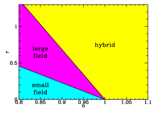
Figure 10: Regions corresponding to the different inflation models in the plot $r$ vs $n_{s}$ [DKK97]

• convex potentials or large field models ($0<\eta<2\epsilon$)

  The potential is typically a single monomial potential:

  $$V(\phi)=\lambda m_{{}_{P}}^{4}\left({\phi\over m_{{}_{P}}}\right)^{n}\ ,$$ (109)

  with $n>1$. Since the slow roll parameters are $\epsilon=n^{2}(m_{{}_{P}}/\phi)^{2}/2$ and $\eta=n(n-1)(m_{{}_{P}}/\phi)^{2}$, the slow roll regime corresponds to $\phi\gg m_{{}_{P}}\sqrt{n(n-1)}$ (for $n>2$). Because the field has a value larger than the Planck scale (hence the name “large field model”), this might seem out of the reach of the effective low energy gravitation theory. But A. Linde [Li83] argued that the criterion is rather $V<m_{{}_{P}}^{4}$; in fact, he suggested that the scalar field emerges from the Planck era with a value $\phi_{0}$ such that $V(\phi_{0})\sim m_{{}_{P}}^{4}$ i.e. $\phi_{0}\sim m_{{}_{P}}/\lambda^{1/n}$. This corresponds to the chaotic inflation scenario, the simplest example of which being a quadratic potential [Li83]. A difficulty is that the COBE normalisation imposes an unnaturally small value for the $\lambda$ coupling: $\lambda\sim(5.3\times 10^{-4}n)^{2n/(n-2)}$. Another drawback is the large value of the field which makes it necessary to include all non renormalisable corrections of order $\left(\phi/M_{{}_{P}}\right)^{n+p}$, unless they are forbidden by some symmetry.

  The limit case in this class is the exponential potential

  $$V(\phi)=V_{0}\exp(-\lambda\phi/m_{{}_{P}})$$ (110)

  which leads to a power law inflation [LM85]: $a(t)\propto t^{2/\lambda^{2}}$. This model yields $\eta=2\epsilon=\lambda^{2}$, hence $r=-8(n_{S}-1)$. It is incomplete since inflation does not end.

  

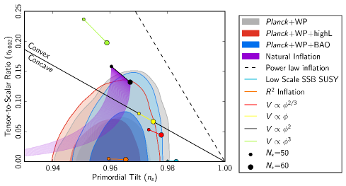
  Figure 11: Constraints set by Planck data on various inflation models in the plot $r$ (evaluated at the pivot scale $k_{*}=0.002$ Mpc^-1) vs $n_{s}$ [Planck13_22]. Small dots correspond to models with $50$ e-foldings, large dots to $60$ e-foldings.

• concave potential or small field models ($\eta<0$)

  In this class, illustrated first by the new inflation scenario [Li82, AS82], the field $\phi$ starts at a small value and rolls along an almost flat plateau (where $V^{\prime\prime}(\phi)<0$) before falling to its ground state. This type of potential, often encountered in symmetry breaking transitions may be parametrized, during the phase transition by:

  $$V(\phi)=V_{0}\left[1-\left({\phi\over\mu}\right)^{p}+\cdots\right]\ ,$$ (111)

  where the dots indicate higher order terms not relevant for inflation. In the same class appears the so-called “natural inflation” potential [BG86, FFO90]

  $$V(\phi)=V_{0}\left[1+\cos(\phi/f)\right]\ .$$ (112)

  A difficulty shared by the class of small field models is the unnaturalness of the initial conditions: why start at the height of the potential, in a plateau region or close to an unstable extremum? In the case of a symmetry breaking potential, the rationale could be thermal: the restoration of the symmetry at high temperature naturally leads to start at the unstable “false vacuum”.

  The first model proposed for inflation [St80] was based on a modification of gravity described by the following action:

  $$S={m_{{}_{P}}^{2}\over 2}\int d^{4}x\sqrt{-\tilde{g}}\left(\tilde{R}+\alpha\tilde{R}^{2}\right)\ ,$$ (113)

  where $\tilde{R}$ is the Ricci scalar associated with the metric $\tilde{g}_{\mu\nu}$. It may be proved that this is equivalent to standard Einstein gravity plus a scalar field with a potential that falls in the same class as we just discussed (see Exercise 2-1).

• hybrid models ($0<2\epsilon<\eta$)

  The field rolls down to a minimum of large vacuum energy (where $V^{\prime\prime}(\phi)<0$) from a small initial value. Inflation ends because, close to this minimum, another direction in field space takes over and brings the system to a minimum of vanishing energy [Li91]. Such models, which thus require several fields, were constructed in order to allow inflation at scales much smaller than the Planck scale. In this case (see (100), $\epsilon$ can be very small and thus $r$ as well. This class of model is the only one that can accomodate values of $n_{S}$ larger than $1$ (i.e. a blue spectrum).

  We note that, for most models, the inflation scale is much larger than the TeV scale. This should in principle lead us to consider inflation models in the context of supersymmetry, in order to avoid an undesirable fine tuning of parameters. In fact, supersymmetric (and superstring) theories are plagued with the presence of numerous flat directions: this might be a blessing for the search of inflation potential. Two such types of potentials rely on the properties of basic supersymmetry multiplets: they are called $F$-term [CLLSW94, St95] and $D$-term [BD96, Ha96] inflation and fall in the category of hybrid inflation. They are not presently favoured by Planck data because they give too large values of $n_{S}$ (of the order of $0.98$).

Exercise 2-1 : We show that a certain class of 4-dimensional models which extend Einstein theory are equivalent to Einstein gravity with a scalar field coupled to the metric (i.e. a scalar-tensor theory). This class of models is described by the following action:

$$S={m_{{}_{P}}^{2}\over 2}\int d^{4}x\sqrt{-\tilde{g}}f(\tilde{R})+S_{m}(\psi,\tilde{g}_{\mu\nu})\ ,$$ (115)

where $\tilde{R}$ is the Ricci scalar associated with the metric $\tilde{g}_{\mu\nu}$, and $f(\tilde{R})$ is a general function of this Ricci scalar. We note that the Starobinsky action (113) corresponds to $f(\tilde{R})=\tilde{R}+\alpha\tilde{R}^{2}$.

Let us consider the more general action:

$$S={m_{{}_{P}}^{2}\over 2}\int d^{4}x\sqrt{-\tilde{g}}\left[f(\chi)+{df\over d\chi}(\tilde{R}-\chi)\right]+S_{m}(\psi,\tilde{g}_{\mu\nu})\ .$$ (116)

a) Show that the variation of (116) with respect to $\chi$ leads to (115).

b) Redefining the metric and the scalar field through

$$g_{\mu\nu}\equiv{df\over d\chi}\tilde{g}_{\mu\nu}\ \ ,\ \ \phi\equiv-\sqrt{{3\over 2}}m_{{}_{P}}\log{df\over d\chi}\ ,$$ (117)

show that one recovers the familiar form of the scalar-tensor gravity:

$$S=\int d^{4}x\sqrt{-g}\left[{m_{{}_{P}}^{2}\over 2}R-{1\over 2}\partial^{\mu}\phi\partial_{\mu}\phi-V(\phi)\right]+S_{m}(\psi,A^{2}(\phi)g_{\mu\nu})\ ,$$ (118)

where one will express the potential $V(\phi)$ in terms of $\chi$, $f(\chi$ and $df/d\chi$, and give the explicit form of $f(\phi)$.

c) Identify the potential $V(\phi)$ in the case of the Starobinsky function $f(\chi)=\chi+\alpha\chi^{2}$.

Hints: a) $\chi=\tilde{R}$, under the condition that $f^{\prime\prime}\not=0$.

b) $V\equiv m_{{}_{P}}^{2}{\chi df/d\chi-f\over 2(df/d\chi)^{2}}$ and $A(\phi)=\exp\left[\phi/(m_{{}_{P}}\sqrt{6})\right]$.

0.3 Light does not say it all (1): the violent Universe

The Universe is the siege of many violent phenomena; one may cite explosions like supernovae, gamma ray bursts (GRB) or the emission of energetic particles by active galaxy nuclei (AGN), quasars, blazars… The time constants $\tau$ associated with the phenomena are very short on the scale of the Universe. For example, a GRB may be visible on the sky only for a few seconds. This means that the distance scales $c\tau$ involved are very small: the distance that light travels in $10$ seconds is only 3 million km, that is $0.002$ astronomical unit ($1$ a.u. is the Sun-Earth distance). Indeed, very compact objects, such as neutron stars or black holes, are at the heart of such violent phenomena. We will start by reviewing the origin of such compact astrophysical objects, which appear at the end of the life of a star.

0.3.1 The end of the life of a star: from white dwarfs to neutron stars and black holes

The evolution of a generic gravitational system such as a star is governed by two competing processes: gravitational forces which tend to contract the system and thermal pressure which is due to the thermonuclear reactions within, which tendto expand the sytem. In a stable star like our Sun at present, the two processes balance each other. But when the nuclear fuel is exhausted, the (core of the) star starts to collapse under the effect of gravity; the gravitational energy thus released heats up the outer layers of the star, which produces the explosive phenomena that we observe.

But what is the fate of the collapsing core? Gravitational pressure is eventually counterbalanced by quantum degeneracy pressure. Let us explain the nature of this pressure. Since matter is made of fermions of spin $1/2$, Pauli principle applies: two fermions cannot be in the same state. Fermionic matter will thus resist at some point to excessive pressure.

Let us be more quantitative. Since there are $4\pi p^{2}dp/(2\pi\hbar)^{3}$ levels per unit volume with momentum between $p$ and $p+dp$ and two spin states per level, the number of fermions per unit volume is given in terms of the maximal momentum by

$$n={2\over(2\pi\hbar)^{3}}\int_{0}^{p_{F}}4\pi k^{2}dk={p_{F}^{3}\over 3\pi^{2}\hbar^{3}}\ .$$ (119)

The energy of the highest level, or Fermi energy $\epsilon_{F}$, is therefore given in terms of the number density $n$. If the particles are non-relativistic, then

$$\epsilon_{F}={p_{F}^{2}\over 2m}={1\over 2}\left(3\pi^{2}\right)^{2/3}\hbar^{2}{n^{2/3}\over m}\ .$$ (120)

On the other hand, the gravitational energy per nucleon of a system of size $R$ and mass $M$ (with $N=4\pi R^{3}n_{N}/3=M/m_{N}$ nucleons) is

$$\epsilon_{g}={G_{{}_{N}}Mm_{N}\over R}=G_{{}_{N}}m_{N}^{2}{N\over R}=\left({4\pi\over 3}\right)^{1/3}G_{{}_{N}}m_{N}^{2}N^{2/3}n_{N}^{1/3}\ .$$ (121)

The Fermi energy starts to dominate over the gravitational energy for

$$n_{N}^{1/3}>{2\over(3\pi^{2})^{2/3}}\left({G_{{}_{N}}m_{N}^{2}m\over\hbar^{2}}\right)N^{2/3}\nu^{2/3},$$ (122)

where $\nu=n_{N}/n$ ($\nu$ depends on the species of the fermions that are degenerate; see below), or

$$RM^{1/3}<{1\over\alpha_{G}}{\hbar\over mc}m_{N}^{1/3}\nu^{-2/3}\ ,$$ (123)

where, as above, $\alpha_{{}_{G}}\equiv(G_{{}_{N}}m_{N}^{2}/\hbar c)\sim 6\times 10^{-39}$.

We see from (122) that gravitational collapse is first stopped by the quantum degeneracy of electrons: the corresponding astrophysical objects are known as white dwarfs. Writing thus $m=m_{e}$ and $\nu=2$ (two nucleons per electron), we find that $RM^{1/3}\sim 10^{-2}R_{\odot}M_{\odot}^{1/3}$. A white dwarf with $M=M_{\odot}$ has radius $R\sim 10^{-2}R_{\odot}$ and density $\rho\sim 10^{6}\rho_{\odot}$. It is more compact than a star.

If density continues to increase, the value of the Fermi energy is such that the fermions are relativistic: it follows from (119) that $p_{F}>mc$ reads $\left(3\pi^{2}\right)^{1/3}\hbar n^{1/3}>mc$ or, using $n=3N/\left(4\pi\nu R^{3}\right)$,

$$R<\left({9\pi\over 4}\right)^{1/3}{\hbar c\over mc^{2}}N^{1/3}\nu^{-1/3}\ .$$ (124)

But, since $\epsilon_{F}\sim p_{F}c=\left(3\pi^{2}\right)^{1/3}\hbar cn^{1/3}$, both $\epsilon_{F}$ and $\epsilon_{g}$ scale like $n^{1/3}$. Quantum degeneracy pressure can overcome gravitational collapse only for $N<3\sqrt{\pi}\alpha_{G}^{-3/2}/(2\nu^{2})$, or

$$M<3\sqrt{\pi}\alpha_{G}^{-3/2}m_{N}/(2\nu^{2})\sim 1\ M_{\odot}/\nu^{2}\ .$$ (125)

This bound is the well-known Chandrasekhar limit for white dwarf masses (a more careful computation gives a numerical factor of $5.87$ [Wei]). The radius of the object then satisfies (see (124))

$$R<{3\sqrt{\pi}\over 2}\alpha_{G}^{-1/2}{\hbar c\over mc^{2}}{1\over\nu}\ .$$ (126)

Setting $m=m_{e}$ gives a limit value of some $10^{4}$ km.

For even higher densities, most electrons and protons are converted into neutrons through inverse beta decay ($p+e^{-}\rightarrow n+\nu$). A new object called neutron star forms when the neutron Fermi energy balances the gravitational energy. Writing $m=m_{n}$ instead of $m_{e}$ in (123), we now have $RM^{1/3}\sim 10^{-5}R_{\odot}M_{\odot}^{1/3}$: a neutron star with $M=M_{\odot}$ has radius $R\sim 10^{-5}R_{\odot}$ and density $\rho\sim 10^{15}\rho_{\odot}$.

The bound (125) obtained above in the case of relativistic fermions (neutrons in this case) is called the Oppenheimer-Volkoff bound: more precisely, the maximal mass of a neutron star is $M=0.7\ M_{\odot}$, with a corresponding radius $R=9.6$ km (cf. (126) with $m=m_{n}$). If the mass is larger, the star undergoes gravitational collapse and forms a black hole.

0.3.2 Gravitational collapse: black holes

Let us first backtrack a little and return to Einstein’s equations (3). Because they are non-linear, there are few solutions known. The first exact non-trivial solution was found in late 1915 by Schwarzschild, who was then fighting in the German army, within a month of the publication of Einstein’s theory and presented on his behalf by Einstein at the Prussian Academy in the first days of 1916 [Sc16], just before Schwarzschild death from a illness contracted at the front. It describes static isotropic regions of empty spacetime, such as the ones encountered in the exterior of a static star of mass $M$ and radius $R$.

The Schwarzschild solution reads, for $r>R$ (see Exercise 3-1),

$$ds^{2}=\left(1-{2G_{{}_{N}}M\over r}\right)dt^{2}-\left(1-{2G_{{}_{N}}M\over r}\right)^{-1}dr^{2}-r^{2}d\theta^{2}-r^{2}\sin^{2}\theta d\phi^{2}\ .$$ (127)

The Schwarzschild solution is singular at $r=R_{S}\equiv 2G_{{}_{N}}M$, a distance known as the Schwarzschild radius. This is not a problem as long as $R_{S}<R$ since this solution describes the exterior region of the star. A different metric describes the interior. On the other hand, we will see in Section 0.3.2 that, in the case where $R<R_{S}$, i.e. $2G_{{}_{N}}M/R>1$, the system undergoes gravitational collapse and turns into a black hole.

Exercise 3-1 : In this exercise, we derive the Schwarzschild solution (127). Because we look for static isotropic solutions, we may always write the spacetime metric as:

$$ds^{2}=e^{2\nu(r)}dt^{2}-e^{2\lambda(r)}dr^{2}-r^{2}\left(d\theta^{2}+\sin^{2}\theta d\phi^{2}\right)\ .$$ (128)

In other words, the only non-vanishing elements of the metric are:

$$g_{tt}=e^{2\nu(r)},\ g_{rr}=-e^{2\lambda(r)},\ g_{\theta\theta}=-r^{2},\ g_{\phi\phi}=-r^{2}\sin^{2}\theta\ .$$ (129)

a) Work out the Christoffel symbols from (242) and the Ricci tensor components from (244).

b) Show that the Einstein’s equations in the vacuum simply amount to a condition of vanishing Ricci tensor:

$$R_{\mu\nu}=0\ .$$ (130)

c) From the vanishing of $R_{tt}$ and $R_{rr}$ and the fact that, at large distance from the star, space should be flat, both $\lambda$ and $\nu$ should vanish at spatial infinity. Hencededuce that

$$\lambda=-\nu\ .$$ (131)

d) From the vanishing of $R_{\theta\theta}$, deduce that

$$g_{tt}=e^{2\nu}=1-{2G_{{}_{N}}M\over r}\ .$$ (132)

Hints: a)

$$R_{tt} = \left(\nu^{\prime\prime}+\nu^{\prime 2}-\lambda^{\prime}\nu^{\prime}+{2\nu^{\prime}\over r}\right)e^{2(\nu-\lambda)}\ ,$$

$$R_{rr} = -\nu^{\prime\prime}-\nu^{\prime 2}+\lambda^{\prime}\nu^{\prime}+{2\lambda^{\prime}\over r}\ ,$$

$$R_{\theta\theta} = 1-\left(1+r\nu^{\prime}-r\lambda^{\prime}\right)e^{-2\lambda}\ ,$$

$$R_{\phi\phi} = R_{\theta\theta}\sin^{2}\theta\ .$$ (133)

b) (3) reads $R_{\mu\nu}-{1\over 2}g_{\mu\nu}R=0$. Contracting with $g^{\mu\nu}$ yields $R=0$.

d) The constant of integration is identified with the mass $M$ because, in the Newtonian limit, $g_{tt}=1+2\Phi$ where $\Phi$ is the Newtonian potential.

Exercise 3-2 : What is the Schwarzschild radius of the sun? of an astrophysical object of mass $3\times 10^{6}\ M_{\odot}$?

Hints: Do not forget that we have set $c=1$. Otherwise, $R_{S}=2G_{{}_{N}}M/c^{2}$, that is $2.95$ km for the sun, $8.85\times 10^{9}$ m $=0.06$ au for an object of mass $3\times 10^{6}\ M_{\odot}$.

We now understand that, when (the core of) a star of mass $M$ in gravitational collapse overcomes the degeneracy pressure of neutrons to reach a size $R<R_{S}=2G_{{}_{N}}M$, nothing seems to drastically change for observers located at distances $r>R_{S}$. However, the behaviour of the Schwarzschild metric 127 appears to be singular: $g_{tt}$ vanishes and $g_{rr}$ diverges. It took some time (Lemaître again!) to realize that this was not the sign of a real singualrity but was just an artifact of the choice of coordinates: other choices lead to a regular behaviour (see Exercise 3-3). The true singularity lies at $r=0$ where the collapsing matter ends up.

In order to understand the nature of the surface at $r=R_{S}$, let us keep for a moment longer the Schwarzschild coordinates and consider sending a light signal radially from some point $r_{1}$ to $r_{2}>r_{1}$ where it is received a time $\Delta t$ later. Since $ds^{2}=0$ (as well as $d\theta=d\phi=0$), we have simply

$$\Delta t=\int_{r_{1}}^{r_{2}}{dr\over\left(1-R_{S}/r\right)}\ .$$ (134)

If $r_{1}<R_{S}$, this is finite only for $r_{2}<R_{S}$, in which case it is simply $r_{2}-r_{1}+R_{S}\ln\left[(R_{S}-r_{2})/(R_{S}-r_{1})\right]$. In other words, signals emitted from within the Schwarschild radius never reach the outside. There is really a breach of communication. Indeed, the surface $r=R_{S}$ is an event horizon (see Section 0.2.1).

Let us take this opportunity to present a classical interpretation of the Schwarzschild radius. Remember that the existence of black holes was conceived by Michell [Mi1784] and Laplace [Laplace] centuries earlier than general relativity. Indeed, the classical condition for escape a body of mass $m$ and velocity $v$ from a spherical star of mass $M$ and radius $R$ is

$${1\over 2}mv^{2}>{G_{{}_{N}}mM\over R}\ .$$ (135)

Thus, not even light ($v=c$) can escape the attraction of the star if $R<2G_{{}_{N}}M/c^{2}$, the Schwarzschild radius.

We note that the Schwarzschild horizon is a fictitious surface, in the sense that an observer crossing this surface would not experience anything particular (we said that there exist coordinates where the behaviour at $R_{S}$ is regular), except deformations due to tidal forces because it comes closer to a very massive object. But once it has crossed this fictitious surface, there is no way to backtrack: the further information that might be gained is lost for ever to the outside world. A useful picture is the one of a person swimming in a river with a waterfall downstream: swimming in the river involves no danger as long as one is safely far from the waterfall, but, at some point the swimmer crosses a fictitious line (the “horizon” of the waterfall) which is the point of no return: even the best swimmer is attracted towards the “singularity” of the waterfall.

So far, our description has been purely classical. Quantum mechanical processes change this picture. Indeed, S. Hawking [Ha75] pointed out that black holes emit radiation through what is known as the process of evaporation. Indeed, it can be shown that an accelerated observer sees a thermal bath of particles at a temperature $T=\hbar a/(2\pi)$ ($a$ being the acceleration): this is the so-called Unruh effect [Un76]. Now, an observer who is at a fixed distance $r>R_{S}$ from the horizon of a black hole in Schwarzschild coordinates has an acceleration $a=R_{S}(1-R_{S}/R)^{1/2}/(2r^{2})$ (see Exercise 3-4). For $r\sim R_{S}$, it thus observes a thermal bath of particles at a temperature measured by an observer at infinity to be

$$T_{H}={\hbar\over 4\pi R_{S}}$$ (136)

The Hawking evaporation process is important to understand the non-observation of primoridal black holes, which would be due to fluctuations of density during the Planck era: such primordial black holes have evaporated.

A final comment using the Schwarzschild coordinates (127): we see that, when $r$ crosses $R_{S}$, the respective signs of $g_{tt}$ and $g_{rr}$ changes. In other words, $t$ becomes a spatial coordinates and $r$ becomes time: the movement towards the central singularity is the clock that ticks.

Exercise 3-3 : Define the Kruskal coordinates $(v,u,\theta,\phi$) related to the Schwarzschild coordinates $(t,r,\theta,\phi)$ through [Kr60]:

$$\hbox{for}\ r>R_{S}\ , u=\left(r/R_{S}-1\right)^{1/2}e^{r/2R_{S}}\cosh(t/2R_{S})\ ,$$

$$v=\left(r/R_{S}-1\right)^{1/2}e^{r/2R_{S}}\sinh(t/2R_{S})\ ,$$

$$\hbox{for}\ r<R_{S}\ , u=\left(1-r/R_{S}\right)^{1/2}e^{r/2R_{S}}\sinh(t/2R_{S})\ ,$$ (137)

$$v=\left(1-r/R_{S}\right)^{1/2}e^{r/2R_{S}}\cosh(t/2R_{S})\ .$$

Deduce from (127) the form of the metric in Kruskal coordinates:

$$ds^{2}={4R_{S}^{3}\over r}e^{-r/R_{S}}\left(dv^{2}-du^{2}\right)-r^{2}\left(d\theta^{2}+\sin^{2}\theta d\phi^{2}\right),$$ (138)

where $r$ is given as an implicit function of $u$ and $v$:

$$\left({r\over R_{S}}-1\right)e^{r/R_{S}}=u^{2}-v^{2}\ .$$ (139)

In order to be more quantitative, let us follow the analysis of Oppenheimer and Snyder [OS39] who were the first to discuss the collapse into a black hole. We consider a fluid of negligible pressure, thus described by the energy-momentum tensor (see (21)) $T_{\mu\nu}=\rho U_{\mu}U_{\nu}$, and study its spherically symmetric collapse.

It turns out that we have already studied this system when we discussed the evolution of a homogeneous and isotropic universe in Section 0.1.3. The metric is given by

$$ds^{2}=d\hat{t}^{2}-a^{2}(\hat{t})\left({d\hat{r}^{2}\over 1-k\hat{r}^{2}}+\hat{r}^{2}d\hat{\theta}^{2}+\hat{r}^{2}\sin^{2}\hat{\theta}d\hat{\phi}^{2}\right)\ ,$$ (140)

as in (19) and the Einstein tensor components are the same as in (246,247). We normalize the coordinate $\hat{r}$ so that $a(0)=1$. Thus

$$\rho(\hat{t})=\rho(0)/a^{3}(\hat{t})$$ (141)

and Einstein’s equations simply read:

$$\dot{a}^{2}+k = {8\pi G_{N}\over 3}{\rho(0)\over a}\ ,$$ (142)

$$\dot{a}^{2}+2a\ddot{a}+k = 0\ .$$ (143)

Assuming that the fluid is initially at rest ($\dot{a}=0$), we obtain from (142)

$$k={8\pi G_{N}\over 3}\rho(0)\ .$$ (144)

Thus, (142) simply reads

$$\dot{a}^{2}(\hat{t})=k\left[a^{-1}(\hat{t})-1\right]\ .$$ (145)

The solution is given by the parametric equation of a cycloid:

$$\hat{t} = {\psi+\sin\psi\over 2\sqrt{k}}\ ,$$

$$a = {1+\cos\psi\over 2}\ .$$ (146)

We see that $a$ vanishes for $\psi=\pi$, that is after a time

$$\tau={\pi\over 2\sqrt{k}}={\pi\over 2}\left({3\over 8\pi G_{{}_{N}}\rho(0)}\right)^{1/2}\ .$$ (147)

Thus a sphere initially at rest with energy density $\rho(0)$ and negligible pressure collapses to a state of infinite energy density in a finite time $\tau$.

In the case of a star of radius $R$ and mass $M$, this solution for the interior of the star should be matched with the Schwarzschild solution (127) describing the exterior. The correspondence between the interior and exterior coordinates is simply $r=Ra(\hat{t})$, $\theta=\hat{\theta}$ and $\phi=\hat{\phi}$, with a more complicate relation between $t$ and $\hat{t}$ (see Ref. [Wei] section 11.9). The first relation ensures that

$$k={2MG_{{}_{N}}\over R^{3}}={R_{S}\over R^{3}}\ ,$$ (148)

in agreement with (144) and $M=(4\pi/3)\rho(0)R^{3}$.

Exercise 3-4 : We consider an observer at rest outside the horizon of a black hole described by the Schwarzschild metric (127) which we write (see Exercise 3-1):

$$ds^{2}=e^{2\nu(r)}dt^{2}-e^{-2\nu(r)}dr^{2}-r^{2}\left(d\theta^{2}+\sin^{2}\theta d\phi^{2}\right)\ .$$ (149)

The observer velocity is $U^{\mu}=\xi^{\mu}/\sqrt{\xi^{2}}$ with $\xi^{\mu}\equiv\delta_{0}^{\mu}$.

a) Show that $\xi_{\mu;\nu}=\xi_{\mu}w_{\nu}-\xi_{\nu}w_{\mu}$, where $w_{\mu}\equiv\partial_{\mu}\nu$ (the covariant derivative $\xi_{\mu;\nu}$ is defined in (245) of Appendix .7).

b) Deduce that the acceleration $A^{\mu}\equiv U^{\rho}\nabla_{\rho}U^{\mu}$ of the observer is simply $A^{\mu}=-w^{\mu}$.

c) Show that the acceleration $a^{2}\equiv-w^{\mu}w_{\mu}$ is given for the observer at fixed $r$, $\theta$ and $\phi$ by

$$a={G_{{}_{N}}M\over r^{2}(1-2G_{{}_{N}}M/r)^{1/2}}\ .$$ (150)

We finally note that, at large distance, the black hole is only caracterized by its mass $M$. Black holes are indeed very simple objects, somewhat similar to particles: Schwarzschild black holes are only characterized by their mass. Other more complex solutions were found later but it was realized that one can only add spin (rotating or Kerr black holes) and charge (charged black holes) but no other independent characteristics: in the picturesque language used by Wheeler, it is said that black holes can have no hair. In a sense, the black holes of general relativity are very similar to fundamental particles, which are caracterized by a finite set of numbers (including mass, spin, and electric charge).

Astrophysical black holes are somewhat more complex because of their material environment, as we will now see.

0.3.3 Astrophysical black holes

For a long time, black holes were considered as a curiosity of general relativity and did not have the status of other stellar objects. This has changed in the last decade which has seen mounting evidence that, at the center of our own galaxy (Milky Way) cluster, there is a massive black hole associated with the compact radio source Sagittarius A^∗. Observations of the motions of nearby stars by the imager/spectrometer NAOS/CONICA working in the infrared [Ot03] have indeed confirmed the presence of a very massive object ($(2.6\pm 0.2).10^{6}$ solar mass) localized in a very small region (a fraction of an astronomical unit, see Fig. 12), which seems only compatible with a black hole.

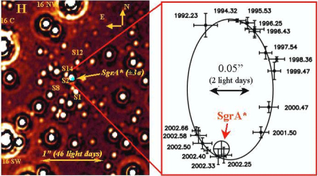
Figure 12: Left: NAOS/CONICA image of the central 2” (Sgr A^∗ in light blue). Right: orbit of the star S2 around Sgr A^∗ [Ot03].

Since then, black holes have been identified in many instances and their role might be central in many phenomena. We have seen that they are very simple gravitational objects. But these simple objects accrete matter, and are thus associated with very diverse phenomena. A picture has emerged, which seems to be valid at very diverse scales (see Fig. 13) of a black hole surrounded by an accretion disk and a torus of dust, with two opposite relativistic jets, which are supposedly formed during the gravitational collapse through a recombination of the magnetic fields. Of course, at the centre of this complex structure, lies the black hole surrounded by its horizon. But the complex phenomena that take place in this surrounding region allow to detect indirectly the black hole.

Let us review some of the astrophysical occurences of black holes.

First, our galaxy is not the only onewhich has a cventral black hole. This is believed to be very general, and in many cases the blck hole and its environment is much more active than our own. Active galaxies are galaxies where the dominant energy output is not due to stars. In the case of Active Galactic Nuclei (AGN), the non-thermal radiation comes from a central region of a few parsecs around the centre of the galaxy. The most famous example of such AGNs is provided by quasi-stellar objects (QSOs) or quasars: these starlike objects turn out to be associated with the point-like optical emission from the nucleus of an active galaxy.

The typology of active extragalactic objects is very complex: radio loud and radio quiet quasars, Seyfert galaxies, BL Lacs or blazars… There has been an effort to build a unified picture [BBR84]: the apparent diversity in the observations would then result from the diversity of perspectives from which we observers see these highly non-isotropic objects. Typically, the model for radio-loud AGNs includes (see Fig. 13, right panel): a central engine, a pair of oppositely directed relativistic jets (cones of semi-angle around $1^{\circ}$) an accretion disk (of size of the order of $1$ parsec), and a torus of material (of size of the order of $100$ parsec) which obscures the central engine when one observes it sideways. Depending on the relative angle between the line of sight and the jet axis, observation may vary in important ways.

Figure 13: Unified picture of the system surrounding an astrophysical black hole in the case of a gamma ray burst (left), a microblazar (centre) and a blazar (right). In the first two cases, the central object is a stellar mass black hole and the size of the accretion disk is about $1000$ km. In the latter (AGN), it is a supermassive black hole of potentially several million solar masses and the accretion disk is of the order of $1$ billion kms.

Gamma ray bursts (GRB) are the most luminous events observed in the universe. They were discovered accidentally by the American military satellites VEGA which were designed to monitor the nuclear test ban treaty of 1963. The first burst was found in 1969, buried in gamma-ray data from 1967: two Vela satellites had detected more or less identical signals, showing the source to be roughly the same distance from each satellite [KSO73].

A GRB explosion can be as luminous as objects which are in our vicinity, such as the Crab nebula, although they are very distant. The initial flash is short (from a few seconds to a few hundred for a long GRB, a fraction of a second for a short one). From 1991 to 2000, BATSE (Burst and Transient Source Experiment) has allowed to detect some 2700 bursts and showed that their distribution is isotropic, a good argument in favor of their cosmological origin. In 1997 (February 28), the precise determination of the position of a GRB (hence named 970228) by the Beppo-SAX satellite allowed ground telescopes to discover a rapidly decreasing optical counterpart, called afterglow. Typically in the afterglow, the photon energy decreases with time as a power law (from X ray to optical, IR and radio) as well as the flux: it stops after a few days or weeks. The study of afterglows gives precious information on the dynamics of GRBs. The launch of the SWIFT satellite on 20 November 2004 has started a new era for the understanding of GRBs.

Given the time scales involved (a few milliseconds for the rise time of the gamma signal), the size of the source must be very small: it cannot exceed the distance that radiation can travel in the same time interval, i.e. at most a few hundred kilometers. Energy must have been ejected in an ultra-relativistic flow which converted its kinetic energy into radiation away from the source: the Lorentz factors involved are typically of the order of $100$!

This flow is collimated and forms a jet of half opening angle $\theta$. The observational evidence for this collimation is an achromatic break in the afterglow light curve: for $t>t_{{\rm jet}}$, it decreases faster than it would in the spherical case [Rh99, SPH99]. If we assume that the relativistic jet, after emitting a fraction $\eta_{\gamma}$ of its kinetic energy into prompt $\gamma$ rays, hits a homogeneous medium with a constant number density $n$, the break appears in the afterglow light curve when the Lorentz factor $\gamma$ becomes of the order of $1/\theta$. This gives a relation between the half opening angle $\theta$ and the break time $t_{{\rm jet}}$ [SPH99]:

$$\theta={0.161\over(1+z)^{3/8}}\left({t_{{\rm jet}}\over 1\ {\rm day}}\right)^{3/8}\left({10^{52}\ {\rm ergs}\over E_{\gamma,{\rm iso}}}\right)^{1/8}\left({n\over 1\ {\rm cm}^{3}}\right)^{1/8}\eta_{\gamma}^{1/8}\ ,$$ (151)

where $E_{\gamma,{\rm iso}}$ is the isotropic equivalent gamma ray energy.

In the collapsar model of Woosley [Wo93], long GRBs are associated with the explosion of a rapidly rotating massive star which collapses into a spinning black hole (see Fig. 13 left panel). The burst and its afterglow have been successfully explained by the interaction of a highly relativistic jet with itself (internal shocks [PX94, RM94]) and with the circumstellar medium (external shocks [RM92]). Typically, one expects per day $10^{6}$ collapses of massive stars in the Universe; $10^{3}$ give rise to a GRB and approximately $1$ of these is pointing towards us its jet. Hence, one may observe from earth about one GRB per day.

Supernovae explosions also provide very bright events in the sky, some of them being visible to the naked eye. Supernovae explosions were thus recorded in 1006, 1054, 1181, 1572 and 1604 . The Sn 1987 A explosion allowed the detection of neutrinos and gamma emission.

The modern theory of supernovae was initiated in the 30s by Baade and Zwicky [BZ34].

Supernovae follow a classification according to spectroscopy. In type I supernovae, hydrogen lines are absent whereas they are present in type II. Moreover, type I has subclasses: for example, type Ia involves intermediate mass elements (Si). Each type corresponds to a different mechanism for the explosion. In particular, type II and type Ia have a completely different interpretation.

We will focus first on type II supernovae.

Presupernova stars ($M>8M_{\odot}$) have an onion-like structure. From the outer to the inner layers, one finds increasingly heavy elements: $H$, $He$, $C$, $O$, $Ne$, $Si$ and $Fe$.

As $Si$ is consumed by nuclear reactions, the mass of the $Fe$ core increases . The resulting density increase then turns the electrons relativistic and makes electronic capture ($p+e\rightarrow n+\nu$) energetically favorable. This diminishes the degenerate electron pressure and leads to the collapse of the core. Since $\rho_{core}\sim 10^{12}$ kg.m^-3, the collapse time is typically $\left(G_{{}_{N}}\rho\right)^{-1/2}\sim 0.1$ s.

This time, neutrinos produced as electrons are turned into neutrons, are trapped in the imploding core. The critical density for which neutrinos are trapped, is typically $\rho\sim 2\times 10^{14}$ kg/m³. As the core is crushed to higher densities, the density approaches that of a neutron star ($\rho\sim 2\times 10^{17}$ kg/m³) and matter becomes almost incompressible. If the process was elastic, the kinetic energy would be enough to bring it back to the initial state. Typically

$$E\sim G_{{}_{N}}M_{core}\left({1\over R_{NS}}-{1\over R_{WD}}\right)\sim{G_{{}_{N}}M_{core}\over R_{NS}}\sim 3\times 10^{46}\ \hbox{J}\ .$$ (152)

This is not completely so but there is a rebound of the core which sends a shock wave outward. Meanwhile, the stellar matter has started to free fall since it is no longer sustained by its core. The falling matter meets the outgoing shock wave and turns it into an accretion wave.

Neutrinos emitted from the core heat up and expand the bubble thus formed. Convection and neutrino heating thus convey a fraction of the order of one percent of the neutron star gravitational mass (152) to the accretion front. This is enough to make it explode.

One word of caution however: numerical models that try to reproduce supernovae explosions have been until now unable to explode the supernovae! One needs to start the explosion artificially. It therefore remains possible that one is still missing a key ingredient in the recipe.

The bulk of the star blown off by the explosion makes what is known as a supernova remnant. It sweeps the interstellar medium at great velocity ($10000$ km/s) and may remain visible for $10^{5}$ to $10^{6}$ years. A large fraction of the interstellar medium is thus swept by supernovae remnants (see Exercise 3-1). This is important since this is believed to be the way the heaviest nuclear elements are scattered in the universe (primordial nucleosynthesis produces no element heavier than ${}^{7}\hbox{Li}$).

Exercise 3-4 : a) Assuming approximately one supernova explosion every 30 years in our galaxy (assimilated to a disk of radius $15$ kpc and thickness $200$ pc), compute the corresponding rate ${\cal R}$ of supernovae explosions per pc³ and per year.

b) If every supernova leads to a remnant of radius $R=100$ pc that lasts for $t\sim 10^{6}$ yrs, what fraction of the galaxy volume is filled by the supernova remnant?

Hints: a) ${\cal R}\sim 2.3\times 10^{-13}$ pc^-3.yr^-1.

b)$1-\exp\left[-(4\pi/3)R^{3}{\cal R}t\right]\sim 0.5$.

SNIa events on the other hand are thermonuclear explosions of white dwarfs. More precisely, a carbon-oxygen white dwarf accretes matter (from a companion star or by coalescence with another white dwarf) which causes its mass to exceed the Chandrasekhar limit. The central core collapses, making the carbon burn and causing a wave of combustion to propagate through the star, disrupting it completely. The total production of energy is thus almost constant. For a white dwarf of radius $1500$ to $2000$ km, about $2\times 10^{51}$ ergs is released in a few seconds during which takes place the acceleration of the material. This is followed by a period of free expansion. Virtually all the energy of the explosion goes into the expansion. The luminosity of the supernova, on the other hand, finds its origin in the nuclear decay of the ${}^{56}\hbox{Ni}$ freshly synthesized. The energy release in the nuclear decays ${}^{56}\hbox{Ni}\rightarrow{}^{56}\hbox{Co}\rightarrow{}^{56}\hbox{Fe}$, with respective lifetimes of $8.8$ and $111$ days, represents a few percent of the initial energy release.

This model allows to understand the homogeneity of the observed type Ia supernovae explosions and why they have been used successfully as standard candles in cosmology (see Section 0.5.1 of Chapter 0.5). The structure of a white dwarf is determined by degenerate electrons and thus independent of detailed chemical composition (see Section 0.3.1). The rate of expansion is set by the total energy available since the complete white dwarf is disrupted. Finally, the absolute brightness is determined by the radioactive decay of ${}^{56}\hbox{Ni}$ produced during the explosion. Less Ni means a lower luminosity but also lower temperature in the gas and thus lower opacity and more rapid energy escape. Thus dimmer supernovae are quicker i.e. have narrower light curves.

0.3.4 High energy cosmic particles

As explained above, compact objects and the violent phenomena associated with their formation are important to understand the origin of high energy cosmic particles. It is important to identify the potential sites of acceleration. Obviously, the jets described in the preceding Section are sources of energetic particles. Shock fronts, such as supernovae remnants, are also the siege of acceleration for particles whose multiple scattering off magnetized clouds lead to multiple encounters with the shock front.

M. Hillas [Hi84] has proposed a general discussion of potential acceleration sites, in terms of the magnetic fields $B$ availalble and the size $R$ of the site. The Larmor radius of the particle $r_{L}=E/(qBc)$ (in relativistic regime) may, with increasing energy $E$, become larger than the dimension $R$ of the accelerating site. We thus have the condition ($q=Ze$)

$$E<E_{{\rm max}}=qBcR=Z\left({B\over 1\ \mu\hbox{G}}\right)\left({R\over 1\ \hbox{Mpc}}\right)9.3\ 10^{20}\hbox{eV}\ .$$ (153)

Note that this is the work of the electric field ${\cal E}=Bc$ over the maximal distance $R$. In the case of acceleration on magnetic clouds or a shock wave (where ${\cal E}=BV$), the maximal energy reads:

$$E_{{\rm max}}=ZeBVR\ .$$ (154)

In the case where acceleration involves large Lorentz factors $\gamma$, an extra factor $\gamma$ should be included to account for the energy being measured in the lab frame (also ${\cal E}=\gamma BV$).

This general criterion allows to draw the now classical Hillas diagram which identifies the possible acceleration sites in a plot $\log\left(B/1\ \hbox{G}\right)$ vs. $\log\left(R/1\ \hbox{km}\right)$. As can be seen on Fig. 14, given species of cosmic particles accelerated at given energies are represented by diagonal lines (from top to bottom on the figure: protons of $10^{21}$ eV, protons of $10^{20}$ eV and iron nuclei of $10^{20}$ eV).

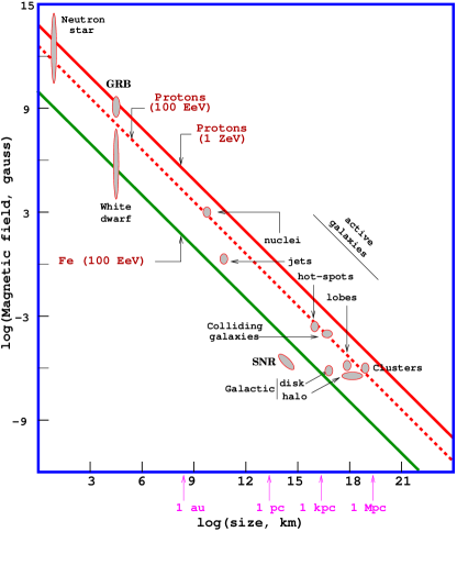
Figure 14: Hillas diagram showing size and magnetic fields of potential acceleration sites. Sites below the diagonal lines cannot accelerate protons above $10^{21}$ eV, protons above $10^{21}$ eV and Fe nuclei above $10^{20}$ eV, respectively from top to bottom.

0.4 Light does not say it all (2): dark matter

We have known for a long time that the Universe has a dark component, and is not only luminous matter and radiation: already in 1933, by studying the velocity distribution of galaxies, Zwicky [Zw33] discovered that the Coma cluster had $400$ times more mass than expected from its luminosity. Through the XX^th century, it was realized that non-luminous matter, dark matter, is needed at all scales from galactic to cosmological. This pleads for a form of matter which is not included in the Standard Model, hence for physics beyond the Standard Model. Indeed, the detection of dark matter might be the first sign of physics beyond the Standard Model. Hence the programs of direct or indirect dark matter detection are of key importance not only for astrophysics but also for high energy physics.

0.4.1 The observational case

As we alluded to above, dark matter was first identified by Fritz Zwicky [Zw33, Zw37] in 1933 when studying the velocity distribution of galaxies in the Coma cluster. Using the virial theorem

$$2\langle E_{{\rm kin}}\rangle=-\langle E_{{\rm pot}}\rangle$$ (155)

(where $\langle\cdots\rangle$ indicates time averaging), he concluded that there is $400$ times more mass than expected from the luminosity.

This was consistently confirmed by the study of the rotation curves of galaxies i.e. the velocity $v(r)$ of stars as function of their distance $r$ to the centre of the galaxy. Using again the virial theorem (155), we have for stars in the outer regions of the galaxy, since $E_{{\rm kin}}\sim mv^{2}$ and $E_{{\rm pot}}\sim G_{{}_{N}}mM/r$ ($m$ is the mass of the star, $M$ of the galaxy),

$$v\propto\sqrt{{G_{{}_{N}}M\over r}}\ .$$ (156)

Thus, one should see the velocity decrease as $r^{-1/2}$ for stars at the border of the galaxy. This is not what is observed. Indeed, the rotation curves of galaxies, which were studied thoroughly through the 60s and 70s showed (see Figure 15) that the velocities do not start decreasing at the border of the luminous galaxy, as if there was more matter beyond. In fact, one needs a factor of order $10$ more matter in spiral galaxies. The extra matter forms a halo that extends beyond the luminous galaxy.

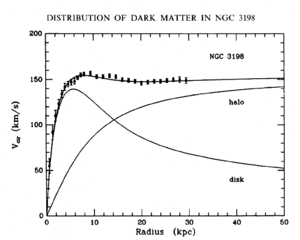
Figure 15: Rotation curve $v(r)$ for the galaxy NGC 3198. The curve labeled “disk” indicates the curve due to the stars in the galaxy, which extend only to $10$ kpc; the curve labeled “halo” is the one that would be due solely to a spherical halo of dark matter.

For example, the modern picture of our own Galaxy, the Milky Way, is one of a luminous bulge of a few kpc at the centre of a disk of radius $12.5$ kpc and thickness $0.3$ kpc, containing some $10^{11}$ stars, surrounded by a nearly spherical halo of dark matter of typical radius $30$ kpc (see Appendix .6 for the definition of a parsec).

But dark matter is not only present in galaxies. We have seen that it was first identified by Zwicky in clusters of galaxy. This is now confirmed by many observation of clusters. X-ray studies have revealed the presence of large amounts of intergalactic gas which is very hot, and hence emits X-rays. The total mass of the gas is greater than that of the galaxies by roughly a factor of two. However this is not enough mass to keep the galaxies within the cluster. Since this gas is in approximate hydrostatic equilibrium with the cluster gravitational field, the mass distribution can be determined, which leads to a total mass estimate approximately six times larger than the mass of the individual galaxies or of the hot gas.

A powerful tool for mapping dark matter is gravitational lensing, which is based on the deflection of light by matter: the light of a distant galaxy is deflected by an accumulation of matter present on the line of sight, just as it is by a lens (see Fig. 16). The deviation of light rays depends on the ratio of distances between observer, lens and source, as well as on the mass of the deflector.

More precisely, the “lens equation” may be with written as (see Fig. 15 for notations):

$${\bf\theta}_{I}={\bf\theta}_{S}+{D_{LS}\over D_{OS}}{\bf\alpha}\ .$$ (157)

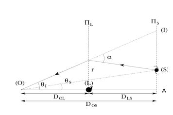
Figure 16: Configuration of a gravitational lens: $S$ is the astrophysical source, $O$ is the observer, $L$ is the (point) lens and $I$ is the image. The source lies at an angle $\theta_{S}$ from the axis $OL$ but is seen at an angle $\theta_{I}$: the deviation angle is thus $\alpha$.

It is well-known that the deflection angle of a light ray passing an object of mass $M$ with an impact parameter $b$ is $\alpha=4G_{{}_{N}}M/(bc^{2})$ (see for example [Schutz] p.286). Hence the lensing effect allows to detect the mass distribution.

Massive clusters may induce multiple images of background galaxies. One then talks of strong lensing [WCOT95]. The shape of a single galaxy can also be deformed into an arclet through lensing. In the case of weak lensing, the effect is measured through the deformation of the shape of galaxies but, because galaxies do not have a circular shape, it can only be measured statistically: galaxies tend through lensing to have aligned shapes [Me99].

Finally, we have seen in Section 0.1.5 that cosmological data shows that dark matter is also needed at the largest scales. An illustration of this is the map of dark matter that the Planck collaboration could draw using the gravitational lensing of the CMB light (see Fig. 17).

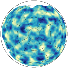
Figure 17: Large scale structures detected by Planck through their lensing potential (galactic North) [Planck13_17]

Since the only proof of existence of dark matter is gravitational (rotation curves, lensing,…), one may wonder whether the observed phenomena are due to a modification of gravity, which would then be different from what general relativity predicts at the corresponding scales. Besides the difficulty of finding a theory that encompasses all the successes of general relativity, the problem is to modify gravity at all the scales where we see signs of dark matter, that is galaxies, clusters of galaxies and cosmological scales.For example, the MOND theory [Mi83a, Mi83b] has been proposed to explain the rotation curves of galaxies but is only Newtonian and requires to be generalized [Be04a] in order to be valid at the scale of the Universe.

The existence of the bullet cluster (see Fig. 18) where two galaxies collide has been presented as a support of dark matter [Cl06] because the luminous parts of the galaxies are displaced with respect to their halos: because dark matter is weakly coupled, the halos (detected through gravitational lensing) continue their way during the collision whereas their luminous matter counterparts (detected through their X-ray emission) are deformed.

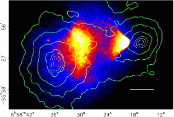
Figure 18: X-ray image of the merging cluster 1E0657-558 obtained by the satellite Chandra, over which is superimposed in green contours the weak lensing reconstruction of the dark matter halos [Cl06].

0.4.2 Dark matter particles

What is dark matter? Since it is nonluminous it is not electrically charged, and the only possible candidate within the Standard Model is the neutrino. But the random motion of neutrinos (the technical term is “free streaming”) would wash out any density fluctuation and prevent the formation of galaxies; one expresses this by saying that neutrinos are hot dark matter. Instead, we need cold dark matter i.e. particles with smaller free streaming length.

Moreover, we need dark matter particles in sufficient quantity. This means that they cannot be in thermal equilibrium today: they must have decoupled from the thermal history of the Universe at some early time. Typically, there are two competing effects to modify the abundance of a species $X$: $X\bar{X}$ annihilation and expansion of the Universe. Indeed, the faster is the dilution associated with the expansion, the least effective is the annihilation because the particles recede from one another. When the temperature drops below the mass $m_{{}_{X}}$, the annihilation rate becomes smaller than the expansion rate and there is a freezing of the number of particles in a covolume. In more quantitative term, this reads for the freezing temperature $T_{f}$:

$$n_{{}_{X}}(T_{f})<\sigma_{{\rm ann}}v>\sim H(T_{f})\ ,$$ (158)

where $<\sigma_{{\rm ann}}v>$ is the thermal average of the $X\bar{X}$ annihilation cross-section times the relative velocity of the two particles annihilating. One finds for the present density (in units of $\rho_{c}$ as usual) (see Ref. [Binetruy] Section 5.5)

$$\Omega_{{}_{X}}h_{0}^{2}\sim{1.07\times 10^{9}\ {\rm GeV}^{-1}\over g_{*}^{1/2}M_{{}_{P}}}\ {x_{f}\over<\sigma_{{\rm ann}}v>}\quad.$$ (159)

where $x_{f}\equiv m_{{}_{X}}/(kT_{f}\sim 20$ and $g_{*}$ is the total number of relativistic degrees of freedom present in the universe at the time of decoupling.

We note that the smaller the annihilation cross section is, the larger is the relic density. We find $\Omega_{X}\sim(100\ \hbox{TeV})^{-2}(\leavevmode\nobreak\ <\sigma_{{\rm ann}}v\leavevmode\nobreak\ >\leavevmode\nobreak\ )^{-1}\sim 0.1\ \hbox{pb}/<\sigma_{{\rm ann}}v>$ (in units where ${/\hskip-5.69054pth}=c=1$, $1$ pb $=2.5\times 10^{-9}$ GeV^-2). This should be compared with the latest result $\Omega_{DM}=0.1187\pm 0.0017$ coming from Planck [Planck13_16].

Thus $\Omega_{{}_{X}}$ will be of the right order of magnitude if $<\sigma_{{\rm ann}}v>$ is of the order of a picobarn, which is a typical order of magnitude for an electroweak process. Also writing dimensionally

$$<\sigma_{{\rm ann}}v>\ \sim{\alpha^{2}\over m_{X}^{2}}\ ,$$ (160)

where $\alpha$ is a generic coupling strength, we find that $\Omega_{{}_{X}}$ is of order 1 for a mass $m_{X}\sim\alpha\times 1000\ \hbox{TeV}$, i.e. in the TeV range. This is why one is searching for a weakly interacting massive particle (or wimp).

There is also the possibility that dark matter particles have produced non-thermally, e.g. from the decay of heavy particles.

A puzzle which is not addressed by the wimp scenario is why dark matter and baryonic matter densities are basically of the same order:

$${\rho_{DM}\over\rho_{B}}\sim 5\ .$$ (161)

Indeed, baryon density arises from baryogenesis (see section 0.1.6) and thus results from a small mismatch between baryons and antibaryons, as seen from (58). On the other hand, the wimp density results from the freezing regime described by (158). There is no reason that the two scenarios lead to similar energy densities, as in (161). This puzzle is addressed by the Asymmetric Dark Matter scenarios (see the review by C. Zurek [Zu13] and references therein). The idea is that dark matter has an asymmetry in the number density of matter over anti-matter similar to the one for baryons:

$$n_{X}-n_{\bar{X}}\sim n_{b}-n_{\bar{b}}\ .$$ (162)

The abundance is therefore approximately one part in $10^{10}$ in comparison with the thermal abundance (see (58)). Eq. (162) suggests that $m_{X}$ is typically $5$ times the proton mass, as a typical baryon mass. Thus generic Asymmetric Dark Matter models tend to favor light dark matter particles.

One may search for dark matter particles through direct detection using their elastic collisions with nuclei $XN\rightarrow XN$ in ultra-low background detectors. The energy of the recoiling nucleus is typically from a few keV to tens of keV. The recoil rate after integration over the dark matter velocity $v$ distribution is

$$R\sim 3.5\times 10^{-2}{\hbox{events}\over\hbox{kg.day}}{100\over A}\left[{100\hbox{GeV}\over m_{{}_{X}}}\times{\sigma_{XN}\over 1\hbox{pb}}\times{\langle v\rangle\over 220\hbox{km.s}^{-1}}\times{\rho\over 0.3\hbox{GeV.cm}^{-3}}\right]\ ,$$ (163)

where $A$ is the atomic mass of the recoil nucleus, $\sigma_{XN}$ the cross-section for dark matter particle-nucleus elastic scattering and $\rho$ the local density of dark matter in our Galaxy. In the case of a neutralino wimp, $\sigma_{XN}$ can be as low as $10^{-12}$ pb, which yields a rate of $10^{-8}$ events/ton.year! Present, and future, experimental limits are shown on Fig. 19. One should note that there is below $10^{-12}$ pb ($10^{-8}$ pb for low-mass particles) an irreducible neutrino background corresponding to the reaction $\nu N\rightarrow\nu N$. Experiments of the next decade should be able to reach this limit.

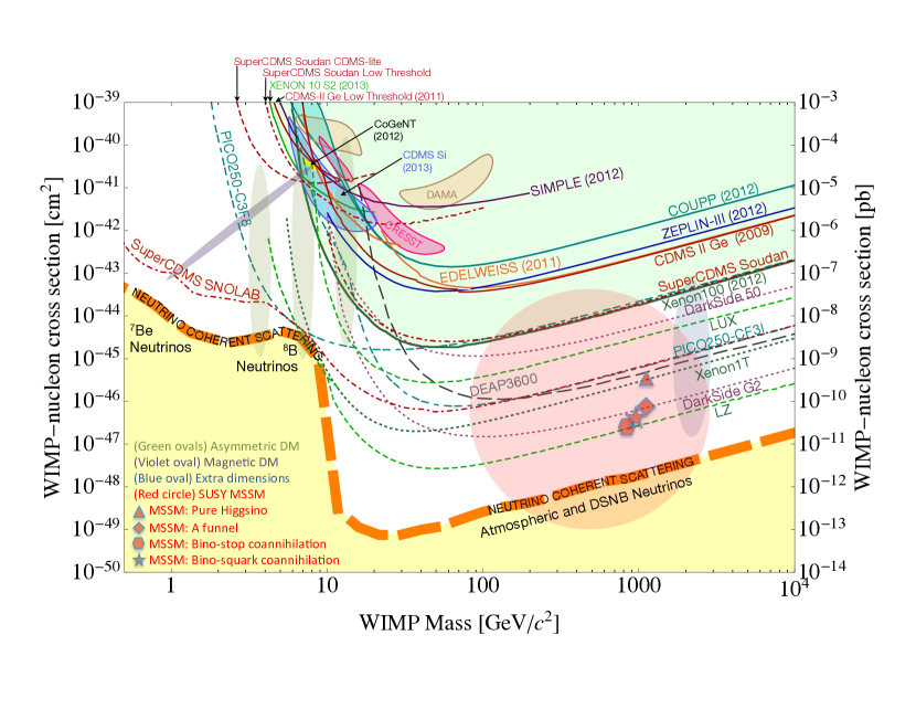
Figure 19: Sensitivities of some running and planned direct detection dark matter experiments to the spin-independent elastic scattering cross-section. Full curves correspond to limits from existing experiments, dashed curves to predicted sensitivities of future experiments. The full brown, pink, blue and yellow regions correspond respectively to the regions allowed by potential signals observed by the DAMA, CREST, CDMS and CoGeNT experiments. The light red disk corresponds to the region favoured by supersymmetric models. The thick yellow line corresponds to the irreducible neutrino background.

Dark matter particles may also be searched for through their annihilation products in massive celestal objects. This is known as indirect detection. Indeed, because they are massive, they tend to accumulate in gravitational potentials, such as the centre of the Sun, or the centre of our Galaxy. They annihilate there into pairs of energetic particles, the energy of which is directly connected with the mass $m_{X}$ of the dark matter particles. One may therefore search for excess of energetic particles (positrons, photons, neutrinos) in the direction of galactic centres such as in our own Milky Way. An excess of energetic positrons (energy of a few tens to few hundred GeV) has actually been observed by the PAMELA, Fermi and AMS-02 experiments. It remains to be seen if this arises from the annihilation of dark matter or from astrophysical sources, such as pulsars: we have seen at the end of Section 0.3 that a certain number of astrophysical sources produce energetic particles. This is indeed a limitation, at least at present, of the indirect detection of dark matter: it needs to be complemented by either direct detection or detection at colliders.

0.4.3 WIMPs and physics beyond the Standard Model

We would like to stress in this section that the presence of a WIMP in a theory is deeply connected with the naturalness of the electroweak scale.

Let us start by recalling what is the naturalness problem (see for example [Binetruy]). As is well-known, the Higgs squared mass $m_{h}^{2}$ receives quadratically divergent corrections. In the context of an effective theory valid up to a cut-off scale $\Lambda$ where a more fundamental theory takes over, $\Lambda$ is the mass of the heavy degrees of freedom of the fundamental theory. Their contribution in loops, quadratic in their mass, destabilizes the Higgs mass and thus the electroweak scale ($m_{h}^{2}\sim\lambda v^{2}$ where $\lambda$ is the scalar self-coupling and $v\sim 1/(G_{{}_{F}}\sqrt{2})^{1/2}\sim 250\ \hbox{GeV}$ is the Higgs vacuum expectation value. More precisely, we have at one loop

$$\delta m_{h}^{2}={3m_{t}^{2}\over 2\pi^{2}v^{2}}\Lambda_{t}^{2}-{6M_{{}_{W}}^{2}+3M_{{}_{Z}}^{2}\over 8\pi^{2}v^{2}}\Lambda_{g}^{2}-{3m_{h}^{2}\over 8\pi^{2}v^{2}}\Lambda_{h}^{2}\ ,$$ (164)

where for completeness we have assumed different cut-offs for the top loops ($\Lambda_{t}$), the gauge loops ($\Lambda_{g}$) and the scalar loops ($\Lambda_{h}$) [BHR06]. The naturalness condition states that the order of magnitude of the Higgs mass is not destabilized by the radiative corrections i.e. $\left|\delta m_{h}^{2}\right|<m_{h}^{2}$. This translates into the conditions:

$$\Lambda_{t} \sim \sqrt{{2\over 3}}\ {\pi v\over m_{t}}m_{h}\sim 3.5m_{h}\ ,$$ (165)

$$\Lambda_{g} \sim {2\sqrt{2}\pi v\over\sqrt{6M_{{}_{W}}^{2}+3M_{{}_{Z}}^{2}}}m_{h}\sim 9m_{h}\ ,$$ (166)

$$\Lambda_{h} \sim {2\sqrt{2}\pi v\over\sqrt{3}}\sim 1.3\ \hbox{TeV}\ .$$ (167)

Thus one should introduce new physics at a scale $\Lambda_{t}\sim 3.5m_{h}$. We will illustrate our argument with two examples: supersymmetry and extra dimensions. In the two cases, one introduces new physics at the scale $\Lambda_{t}$ (supersymmetric particles or Kaluza-Klein modes).

Typically, these models require the presence of a symmetry that prevents direct coupling between the Standard Model (SM) fermions and the new fields that one has introduced: otherwise, such couplings introduce new mixing patterns incompatible with what is observed in flavor mixings (compatible with the Standard Model). This symmetry is usually a parity (i.e. a discrete symmetry) which is the low energy remnant of a continuous symmetry which operates at the level of the underlying fundamental theory: SM fermions are even under this parity whereas the new fields are odd. Among these new fields, the lightest odd-parity particle (we will refer to it as the LOP) is stable: it cannot decay into SM fermions because of the parity; it cannot decay into the new fields because it is the lightest. It is massive and weakly interacting. It thus provides an adequate candidate for a WIMP.

Let us take our examples in turn. In the case of supersymmetry, the parity operation is R-parity (which usually proceeds from a continuous R-symmetry broken by gaugino masses i.e. supersymmetry breaking). And the LOP is the Lightest Supersymmetric Particle, the famous LSP, the lightest neutralino in the simplest models.

In the case of extra dimensions, say a $5$-dimensional model, the local symmetry is $5$-dimensional Lorentz invariance. It ensures conservation of the Kaluza-Klein levels: if $A^{(n)}$ is the $n$th Kaluza-Klein mode of the massless $5$-dimensional field $A$ (in other words, the $4$-dimensional field with mass $m=n/R$, where $R$ is the radius of the $5$th dimension), then in the reaction $A^{(n)}+B^{(p)}\rightarrow C^{(q)}+D^{(r)}$, we have $n+p=q+r$. At energies smaller than $R^{-1}$, this turns into a Kaluza-Klein parity $(-1)^{n}$. The LOP is then the lightest Kaluza-Klein mode, usually $B^{(1)}$, the first mode of the $U(1)_{Y}$ gauge boson [ST02].

In realistic models, there is often the possibility that other odd-parity fields are almost degenerate in mass with the LOP. This leads to the possibility of co-annihilations, that is annihilations of the LOP against these almost degenerate fields, and to a modification of the relic density in the corresponding region of parameter space.

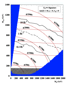
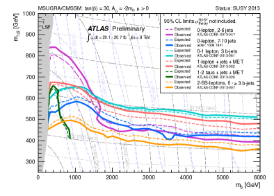
Figure 20: Upper panel: Contours in a parameter space of supersymmetry models in the plot ($m_{0}$, $m_{1/2}$) for the discovery of the missing energy plus jets signature of new physics by the ATLAS experiment at the LHC. The three sets of contours correspond to levels of integrated luminosity at the LHC (in fb^-1), contours of constant squark mass, and contours of constant gluino mass [To02].
Lower panel: Exclusion limits at $95\%$ CL for $8$ TeV, $20$ fb^-1 integrated luminosity analyses in the ($m_{0}$, $m_{1/2}$) plane for the MSUGRA/CMSSM model with the remaining parameters set to $\tan\beta=30,A_{0}=-2m_{0},\mu>0$. Part of the model plane accommodates a lightest neutral scalar Higgs boson mass of 125 GeV [ATLAS_SUSY13].

Searches at LHC are based on the missing energy signal corresponding to the LSP (see Fig. 20). Since LSP are produced in pairs, they are difficult to reconstruct in all generality. But, in the case of a specific model, one may be able to reconstruct the mass of the LSP as well as the relic density.

0.4.4 Other candidates for dark matter

Among the many other candidates proposed for dark matter, one may single out the axion field since it is introduced to solve one puzzle of the Standard Model known as the strong CP problem, which remains to be solved. Moreover, from the point of view of cosmology, this is an interesting illustration of a low-mass and wery weakly interacting particle, as we will encounter in the next Chapter.

As we have already seen, CP symmetry is violated in weak interactions. But the symmetries of the Standard Model allow as well a CP-violating term in the QCD Lagrangian $(\theta g^{2}/32\pi^{2})G^{a}_{\mu\nu}\tilde{G}^{a\mu\nu}$, where $G^{a}_{\mu\nu}$ is the gluon field strength and $g$ the QCD gauge coupling. For non-zero quark masses, this term leads to unobserved CP-violating effects in the strong sector.

The most common way to solve the puzzle is to introduce a scalar field $a(x)$ called axion, with Lagrangian

$${\cal L}_{a}={1\over 2}\partial^{\mu}a\partial_{\mu}a+{g^{2}\over 32\pi^{2}}{a(x)\over f_{a}}G^{a}_{\mu\nu}\tilde{G}^{a\mu\nu}\ ,$$ (168)

where $f_{a}$ is an energy scale, called the axion decay constant (by analogy with the pion decay constant). Strong interactions generate an effective potential for $a(x)$ whose minimum corresponds to no violation of CP. The non-renormalisable interaction $aG\cdot\tilde{G}$ is obtained as the low energy effect of the breaking of a $U(1)$ global symmetry, known as the Peccei-Quinn symmetry [PQ77a, PQ77b], spontaneously broken at the scale $f_{a}$: the axion is the pseudo-Goldstone boson associated with this breaking [We78, Wi78].

The axion mass is

$$m_{a}\sim 6.10^{-6}\ \hbox{eV}\left({10^{12}\hbox{GeV}\over f_{a}}\right)\ .$$ (169)

Its coupling to ordinary matter is proportional to $1/f_{a}$ and can be calculated in specific models. It couples to leptons and to photons, the latter being of the form

$${\cal L}_{a\gamma\gamma}=-g_{a\gamma}{\alpha\over\pi}{a(x)\over f_{a}}\ {\bf E}.{\bf B}\ ,$$ (170)

where ${\bf E}$ and ${\bf B}$ are the electric and magnetic fields, $\alpha$ is the fine structure constant and $g_{a\gamma}$ is a model-dependent coefficient of order $1$. Moreover, since $m_{a}\ll\Lambda_{QCD}$, the axion coupling to quarks should be described through its coupling to hadrons, which occurs through small mixing with the $\pi_{0}$ and $\eta$ mesons. All of these interactions can play a role in searches for the axion, and allows the axion to be produced or detected in the laboratory and emitted by the sun or other stars. Its non-discovery leaves us with an axion window $10^{-6}$ eV $<m_{a}<3.10^{-3}$ eV, or correspondingly, $2.10^{9}$ GeV $<f_{a}<6.10^{12}$ GeV.

Let us describe briefly the cosmology of the axion field (see the review by P. Sikivie [Si08] for a more thorough treatment). The breaking of the $U(1)$ symmetry corresponds to a phase transition, known as the Peccei-Quinn phase transition, at a temperature of order $f_{a}$. This phase transition is characterized by the formation of comic strings.

If the reheat temperature after inflation is smaller than $f_{a}$, then one starts the evolution in the reheated universe with an homogeneous axion field. When the temperature reaches the QCD scale, the effective potential turns on and the axion acquires a mass. At a time $t_{*}\sim m_{a}^{-1}$ ($T_{*}\sim 1$ GeV), the axion starts to oscillate around its minimum. These oscillations do not dissipate into other forms of energy, and thus contribute to the cosmological energy density an amount

$$\Omega_{a}\left({h_{0}\over 0.7}\right)^{2}\sim 0.15\left({f_{a}\over 10^{12}\hbox{GeV}}\right)^{7/6}\left({a(t_{*})\over f_{a}}\right)^{2}\ ,$$ (171)

where $a(t_{*})$ is the axion value at $t_{*}$, which measures the misalignment of the axion with respect to its final minimum. Such a contribution is thus called vacuum realignment.

If the reheat temperature is larger than $f_{a}$, then the cosmic strings produced at the Peccei-Quinn phase transition become at time $t_{*}$ the boundaries of domain walls. This leads to a potential domain wall problem (too much energy stored in the domain walls). There is a certain number of cases where this can be avoided. In this case [Si08],

$$\Omega_{a}\left({h_{0}\over 0.7}\right)^{2}\sim 0.7\left({f_{a}\over 10^{12}\hbox{GeV}}\right)^{7/6}\ .$$ (172)

0.5 Light does not say it all (3): dark energy

We have seen in the introduction that the observation of the acceleration of the expansion of the Universe in 1998-1999 provided a way out of an increasingly uncomfortable tension between models and observation. On one hand, the observed (luminous and dark) matter could account for only a fraction of the critical density $\rho_{c}=10^{-26}$ kg/m³ (other forms of energy being negligible at present time). On the other hand, the standard theory of inflation erased any curvature and naturally led to a spatially flat universe for which $\rho=\rho_{c}$. The discovery of the acceleration of the expansion led to introduce a new component, named dark energy, of a type unknown so far since all known forms of energy (non-relativistic matter, radiation) decelerate the expansion.

In this last chapter, after briefly reviewing the observational case, we will illustrate dark energy models with the example of quintessence, identify some of the problems posed by dark energy models, and the fundamental questions associated with the acceleration of the expansion of the Universe.

0.5.1 Acceleration of the expansion of the Universe: supernovae of type Ia as standard candle

The approach that has made the first case for the acceleration of the expansion of the Universe uses supernovae of type Ia as standard candles (see Section 0.3.3). Two groups, the Supernova Cosmology Project [SCP99] and the High-$z$ Supernova Search [HZS98a] have found that distant supernovae appear to be fainter than expected in a flat matter-dominated Universe. If this is to have a cosmological origin, this means that, at fixed redshift, they are at larger distances than expected in such a context and thus that the Universe expansion is accelerating.

More precisely, one uses the relation (253) between the flux $\phi$ received on Earth and the luminosity $L$ of the supernova. Traditionally, flux and luminosity are expressed on a log scale as apparent magnitude $m_{B}$ and absolute magnitude $M$ (magnitude is $-2.5\ \log_{10}$ luminosity + constant). The relation then reads

$$m_{B}=5\log(H_{0}d_{L})+M-5\log H_{0}+25.$$ (173)

The last terms are $z$-independent, if one assumes that supernovae of type Ia are standard candles; they are then measured by using low $z$ supernovae. The first term, which involves the luminosity distance $d_{L}$, varies logarithmically with $z$ up to corrections which depend on the geometry, more precisely on $q_{0}$ for small $z$ as can be seen from (256). This allows to compare with data cosmological models with different components participating to the energy budget, as can be seen from Fig. 21.

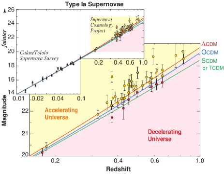
Figure 21: Hubble plot (magnitude versus redshift) for Type Ia supernovae observed at low redshift by the Calan-Tololo Supernova Survey and at moderate redshift by the Supernova Cosmology Project.

In the case of a model with matter and cosmological constant as dominant components, $q_{0}=\Omega_{{}_{M}}/2-\Omega_{\Lambda}$ and the measurement can be turned into a limit in the $\Omega_{M}-\Omega_{\Lambda}$ plane see Fig. 22).

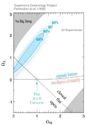
Figure 22: Best-fit coincidence regions in the $\Omega_{M}-\Omega_{\Lambda}$ plane, based on the analysis of 42 type Ia supernovae discovered by the Supernova Cosmology Project [SCP99].

Let us note that this combination $\Omega_{{}_{M}}/2-\Omega_{\Lambda}$ is ‘orthogonal’ to the combination $1-\Omega_{k}=\Omega_{M}+\Omega_{\Lambda}$ measured in CMB experiments. The two measurements are therefore complementary: this is sometimes referred to as ‘cosmic complementarity’.

An important question raised by the analysis above is whether supernovae are truly standard candles. Otherwise, the observation could be interpreted as an history effect: for some reasons, older supernovae would be dimmer. Indeed, strictly speaking, supernovae of type Ia are not standard candles: dimmer supernovae are quicker (see Section 0.3.3). In practice, one thus has to correct the light curves using a phenomenological stretch factor. It is thus more precise to state that supernovae of type Ia are standardizable candles. Moreover, the type of measurement discussed above is sensitive to many possible systematic effects (evolution besides the light-curve timescale correction, presence of dust, etc.), and this has fuelled a healthy debate on the significance of supernova data as well as a thorough study of possible systematic effects by the observational groups concerned.

0.5.2 Cosmological constant and vacuum energy

An obvious solution to the acceleration of the expansion is the introduction of a cosmological constant (see (45) remembering that $q_{0}$ is a deceleration parameter). But there is a severe conceptual problem associated with the cosmological constant, which we now describe.

Considering (25) in flat space at present time implies the general following constraint on $\lambda$:

$$|\lambda|\leq H_{0}^{2}\ .$$ (174)

In other words, the length scale $\ell_{\Lambda}\equiv|\lambda|^{-1/2}$ associated with the cosmological constant must be larger than the Hubble length $\ell_{H_{0}}\equiv cH_{0}^{-1}=h_{0}^{-1}.10^{26}$ m, and thus be a cosmological distance.

This is not a problem as long as one remains classical: $\ell_{H_{0}}$ provides a natural cosmological scale for our present Universe. The problem arises when one tries to combine gravity with the quantum theory. Indeed, from Newton’s constant and the Planck constant $\hbar$, we can construct the (reduced) Planck mass scale

$$m_{{}_{P}}=\sqrt{\hbar c/(8\pi G_{{}_{N}})}=2.4\times 10^{18}\;{\rm GeV/c}^{2}\ .$$ (175)

The corresponding length scale is the Planck length

$$\ell_{{}_{P}}={\hbar\over m_{{}_{P}}c}=8.1\times 10^{-35}\;{\rm m}\ .$$ (176)

The above constraint now reads:

$$\ell_{\Lambda}\equiv|\lambda|^{-1/2}\geq\ell_{H_{0}}={c\over H_{0}}\sim 10^{60}\ \ell_{{}_{P}}\ .$$ (177)

In other words, there are more than sixty orders of magnitude between the scale associated with the cosmological constant and the scale of quantum gravity.

A rather obvious solution is to take $\lambda=0$. This is as valid a choice as any other in a pure gravity theory. Unfortunately, it is an unnatural one when one introduces any kind of matter. Indeed, set $\lambda$ to zero but assume that there is a nonvanishing vacuum (i.e. ground state) energy: $<T_{\mu\nu}>=\rho_{{\rm vac}}g_{\mu\nu}$; then the Einstein equations (3) read

$$R_{\mu\nu}-{1\over 2}g_{\mu\nu}R=8\pi G_{{}_{N}}T_{\mu\nu}+8\pi G_{{}_{N}}\rho_{{\rm vac}}g_{\mu\nu}\ .$$ (178)

As first noted by Zel’dovich [Ze68], the last term is interpreted as an effective cosmological constant (from now on, we set $\hbar=c=1$):

$$\lambda_{{\rm eff}}=8\pi G_{{}_{N}}\rho_{{\rm vac}}\equiv{\Lambda^{4}\over m_{{}_{P}}^{2}}\ .$$ (179)

Generically, $\rho_{{\rm vac}}$ receives a non-zero contribution from symmetry breaking: for instance, the scale $\Lambda$ would be typically of the order of $100$ GeV in the case of the electroweak gauge symmetry breaking or $1$ TeV in the case of supersymmetry breaking. Moreover, it is divergent in the context of the (non-renormalizable) theory of gravity, which would thus favour a value as large as the Planck scale. But the constraint (177) now reads:

$$\Lambda\leq 10^{-30}\;m_{{}_{P}}\sim 10^{-3}\ {\rm eV}.$$ (180)

It is this very unnatural fine-tuning of parameters (in explicit cases $\rho_{{\rm vac}}$ and thus $\Lambda$ are functions of the parameters of the theory) that is referred to as the cosmological constant problem, or more accurately the vacuum energy problem.

If the acceleration observed is indeed due to the cosmological constant, its value is as large as the upper bounds obtained in the previous subsection allow:

$$\lambda\sim H_{0}^{2}\ ,\quad\ell_{\Lambda}\sim\ell_{H_{0}}\ ,\quad\Lambda\sim 10^{-3}\ \hbox{eV}\ .$$ (181)

Regarding the latter scale $\Lambda$, which characterizes the vacuum energy ($\rho_{{\rm vac}}\equiv\Lambda^{4}$), one may note the interesting numerical coincidence:

$${1\over\Lambda}\sim\sqrt{\ell_{H_{0}}\ell_{{}_{P}}}\sim 10^{-4}\ {\rm m}\ .$$ (182)

This relation underlines the fact that the vacuum energy problem involves some deep connection between the infrared regime (the infrared cut-off being $\ell_{H_{0}}$) and the ultraviolet regime (the ultraviolet cut-off being $\ell_{{}_{P}}$), between the infinitely large and the infinitely small.

As an illustration of what such a relation could tell us about some very fundamental aspects of physics (if it is not a mere numerical coicidence), we will follow the approach developed by T. Padmanabhan [Pa08]. As we will discuss later, the value of the cosmological constant might be related to the way that the short distance theory reacts to long distance fluctuations. Let us consider a 3-dimensional domain of size $L$ (e.g. the horizon $\ell_{H_{0}}$). From the point of view of the quantum theory, it consists of $N=(L/\ell_{{}_{P}})^{3}$ elementary cells. For each individual cell, a “natural value” for the energy stored is provided by the scale $m_{{}_{P}}$ characteristic of quantum gravity. This yields

$$\rho\sim{m_{{}_{P}}\over\ell_{{}_{P}}^{3}}\sim{1\over\ell_{{}_{P}}^{4}}\ ,$$ (183)

which is some 120 orders of magnitude larger than observed.

Alternatively, if a mechanism, yet to be determined, cancels this bulk energy, vacuum energy may be produced by the energy fluctuations. The Poissonian fluctuation in energy is $\Delta\epsilon\sim 1/\ell_{{}_{P}}$, which corresponds to an energy for overall fluctuations $\Delta E^{2}\sim N/\ell_{{}_{P}}^{2}$, or an energy density

$$\rho\sim{\sqrt{N}\over\ell_{{}_{P}}L^{3}}\sim{1\over\ell_{{}_{P}}^{5/2}L^{3/2}}\ ,$$ (184)

which again does not reproduce (182) ($\rho_{{\rm vac}}=\Lambda^{4}$).

If we make the further assumption that the relevant degrees of freedom lie on the surface (as the degrees of freedom of a black hole lie on the horizon), then $N=(L/\ell_{{}_{P}})^{2}$ and

$$\rho\sim{\sqrt{N}\over\ell_{{}_{P}}L^{3}}\sim{1\over\ell_{{}_{P}}^{2}L^{2}}\ ,$$ (185)

which is fully consistent with (182). Is this telling us something on the quantization of spacetime, hence of gravity? We will return to this question below.

0.5.3 Supersymmetry

The most natural reason why vacuum energy would be vanishing is a symmetry argument. It turns out that, among the various spacetime symmetries available, global supersymmetry is the symmetry intimately connected with the vanishing of the vacuum energy.

We recall that supersymmetry is a symmetry between bosons and fermions which plays an important rôle in high energy physics, mainly because, through a cancellation between the boson and the fermion fields, it controls severely the quantum fluctuations. Many believe that the Standard Model is the effective theory of a more fundamental theory valid at higher energies, with more boson and fermion fields. These fields should, to some level, make themselves known through the quantum energy fluctuations to which they participe. The fact that we find no trace of them seems to suggest that these fluctuations are tightly constrained, i.e. that the underlying theory is supersymmetric.

Among the various spacetime symmetries, supersymmetry is rather unique. Indeed, in the same way as the generator of time and space translations is the 4-momentum operator $P^{\mu}\equiv(P^{0}=H,P^{i})$, and the generator of spacetime rotations is the tensor $M^{\mu\nu}$, the only other generators carrying a Lorentz index are the generators of supersymmetry $Q_{r}$, where $r$ is a spinor index. In fact, the combination of two supersymmetry transformations is merely a translation in spacetime. This is expressed by the following algebra:

$$\{Q_{r},\bar{Q}_{s}\}=2\gamma^{\mu}_{rs}\ P_{\mu}\ ,$$ (186)

where $\bar{Q}\equiv Q\gamma^{0}$ and $\gamma^{\mu}$ are the gamma matrices introduced by Dirac to write a relativistic fermion (electron) equation. Since the generator of time translations $P_{0}$ is the Hamiltonian $H$, we may easily infer from (186) an expression for the Hamiltonian of the system:

$$H={1\over 4}\sum_{r}Q_{r}^{2}\quad.$$ (190)

It follows that the energy of the vacuum $|0\rangle$ can be expressed as:

$$\langle 0|H|0\rangle={1\over 4}\sum_{r}\parallel Q_{r}|0\rangle\parallel^{2}\ .$$ (191)

Thus, the vacuum energy vanishes if and only if supersymmetry is a symmetry of the vacuum: $Q_{r}|0\rangle=0$ for all $r$.

The problem however is that, at the same time, supersymmetry predicts equal boson and fermion masses and therefore needs to be broken since this is not observed in Nature. The amount of breaking necessary to push the supersymmetric partners high enough not to have been observed yet, typically $\Lambda\sim$ TeV, is incompatible with the limit (180).

Moreover, in the context of cosmology, we should consider supersymmetry in a gravity context and thus work with its local version, supergravity (following (186), local supersymmetry transformations are associated with local spacetime translations which are nothing but the reparameterizations which play a central role in general relativity). In this context, the criterion of vanishing vacuum energy is traded for one of vanishing mass for the gravitino, the supersymmetric partner of the graviton (which allows to cancel the constant vacuum energy at the expense of generating a mass $m_{{}_{3/2}}$ for the gravitino field; see e.g. Ref. [Binetruy], section 6.3 for a more complete treatment). Local supersymmetry is then absolutely compatible with a nonvanishing vacuum energy, preferably a negative one (although possibly also a positive one). This is both a blessing and a problem: supersymmetry may be broken while the cosmological constant remains small, but we have lost our rationale for a vanishing, or very small, cosmological constant and fine-tuning raises again its ugly head.

In some supergravity theories, however, one may recover the vanishing vacuum energy criterion.

0.5.4 Why now?

In the case where the acceleration of the expansion is explained by a cosmological constant, one has to explain why this constant contribution appears to start to dominate precisely now. This is the “Why now?” or cosmic coincidence problem summarized in Fig. 23, the coincidence being between the onset of acceleration and the present time (on the scale of the age of the Universe). In order to avoid any reference to us (and hence any anthropic interpretation, see below), we may rephrase the problem as follows. Why does the dark energy starts to dominate at a time $t_{\Lambda}$ (redshift $z_{\Lambda}\sim 1$) which almost coincides with the epoch $t_{G}$ (redshift $z_{G}\sim 3$ to $5$) of galaxy formation?

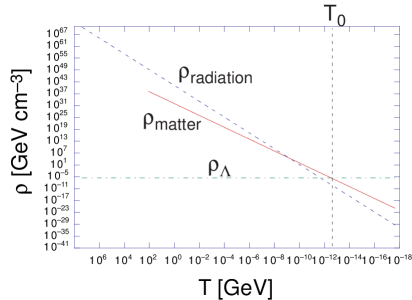
Figure 23: The cosmic coincidence problem illustrated in the case of a cosmological constant

Exercise 5-1 : In this exercise, we will study the evolution of a flat ($k=0$) universe with a non-relativistic matter component (energy density $\rho_{{}_{M}}$) and a cosmological term (or equivalently vacuum energy density $\rho_{\Lambda}=\lambda/(8\pi G_{{}_{N}})$). The relevant equations of evolution are obtained from (23), (29) and (31):

$$H={\dot{a}^{2}\over a^{2}} = {8\pi G_{{}_{N}}\over 3}(\rho_{{}_{M}}+\rho_{\Lambda})\ ,$$ (192)

$${\ddot{a}\over a} = -{4\pi G_{{}_{N}}\over 3}(\rho_{{}_{M}}-2\rho_{\Lambda})\ ,$$ (193)

$$\dot{\rho}_{{}_{M}} = -3H\rho_{M}\ .$$ (194)

a) Defining $H_{\Lambda}\equiv\left(8\pi G_{{}_{N}}\rho_{\Lambda}/3\right)^{1/2}$, show that the solution to the system of equations is given by

$$a(t)=C\left(\sinh{3\over 2}H_{\Lambda}t\right)^{2/3}\ ,$$ (195)

where $C$ is a constant. Compute the Hubble parameter $H$ as well as the ratio $\rho_{{}_{M}}/\rho_{\Lambda}$ as a function of time $t$ and $H_{\Lambda}$.

b) Compute the present Hubble constant $H_{0}$ in terms of $H_{\Lambda}$ and $\Omega_{{}_{M}}$. What is the age of the Universe $t_{0}$ in terms of $H_{0}$ and $\Omega_{{}_{M}}$?

c) Plot $a(t)/C$ and $\rho_{{}_{M}}/\rho_{\Lambda}$ in terms of time. When is the equality between matter and vacuum energy reached? Hints: a) $H=H_{\Lambda}/\tanh(3H_{\Lambda}t/2)$ and $\rho_{{}_{M}}/\rho_{\Lambda}=\left[\sinh(3H_{\Lambda}t/2)\right]^{-2}$.

b) $H_{0}=H_{\Lambda}/\sqrt{1-\Omega_{{}_{M}}}$,

$$t_{0}={2\over 3H_{0}}{1\over\sqrt{1-\Omega_{{}_{M}}}}\ln{1+\sqrt{1-\Omega_{{}_{M}}}\over\sqrt{\Omega_{{}_{M}}}}\ .$$ (196)

0.5.5 More dynamics: dark energy vs modification of gravity

An alternate possibility is that the cosmological constant is much smaller or even vanishing and that the acceleration is due to some new form of energy –known as dark energy– or some modifications of gravity. These two possibilities correspond to modifications of either sides of Einstein’s equations (3). Let us envisage briefly these two cases.

First, we may try to identify a new component $\rho_{{}_{X}}$ of the energy density with negative pressure:

$$p_{{}_{X}}=w_{{}_{X}}\rho_{{}_{X}},\;\;w_{{}_{X}}<0\ .$$ (197)

Note that the equation of state parameter $w_{{}_{X}}$ may not be constant and may thus evolve with time.

Observational data constrains such a dynamical component, referred to in the literature as dark energy, just as it did with the cosmological constant. For example, in a spatially flat Universe with only matter and this unknown component $X$, one obtains from (31) with $\rho=\rho_{M}+\rho_{{}_{X}}$, $p=w_{{}_{X}}\rho_{{}_{X}}$ the following form for the Hubble parameter and the deceleration parameter (compare with (43) and (46))

$$H^{2}(z) = H_{0}^{2}\left[\Omega_{{}_{M}}(1+z)^{3}+\Omega_{{}_{X}}(1+z)^{3(1+w_{{}_{X}})}\right]\ ,$$ (198)

$$q(z) = {H_{0}^{2}\over 2H(z)^{2}}\left[\Omega_{{}_{M}}(1+z)^{3}+\Omega_{{}_{X}}(1+3w_{{}_{X}})(1+z)^{3(1+w_{{}_{X}})}\right]\ ,$$ (199)

where $\Omega_{X}=\rho_{{}_{X}}/\rho_{c}$. At present time (compare with (45)),

$$q_{0}={\Omega_{M}\over 2}+(1+3w_{{}_{X}}){\Omega_{{}_{X}}\over 2}\ .$$ (200)

The acceleration of the expansion observed requires that $\Omega_{{}_{X}}$ dominates with $w_{{}_{X}}<-1/3$.

In Fig. 24, we present constraints in the $(\Omega_{{}_{M}},w_{{}_{X}})$ plane, obtained recently [SNLS11] from combining observations using supernovae and BAO as well as CMB results from WMAP.

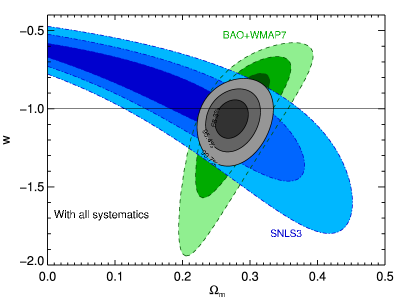
Figure 24: Confidence contours in the $(\Omega_{{}_{M}},w_{{}_{X}})$ plane arising from supernova results from SuperNova Legacy Survey (SNLS) 3 year results (in blue) and combined BAO/WMAP7 constraints (in green) [see Ref. [SNLS11]].

An important property of dark energy is that it does not appear to be clustered (just as a cosmological constant). Otherwise, its effects would have been detected locally, as is the case for dark matter. This points towards scalar fields, which generically have this property. Indeed, an attractive property of scalar fields is that they easily provide a diffuse background by resisting gravitational attraction. The key quantity when discussing gravitational clustering is the speed of sound defined as

$$c_{s}^{2}\equiv{\delta p\over\delta\rho}\ .$$ (202)

It is a measure of how the pressure of the field resists gravitation clustering. In most models of dark energy, we have $c_{s}^{2}\sim 1$, which explains why such scalar dark energy does not cluster: its own pressure resists gravitational collapse.

It should be stressed that, until recently, no fundamental scalar field had been observed in Nature. The discovery of a Higgs particle at the LHC high energy collider has obviously promoted the status of fundamental scalar particles.

In the next section, we will illustrate the dynamics of dark energy on the example of a scalar field evolving with time along its potential. This is often referred to as quintessence. Such scalar fields turn out to be extremely light: the only dimensionful parameter in the problem being the Hubble constant $H_{0}$, their mass is $\hbar H_{0}\sim 10^{-33}\ {\rm eV}$ (see e.g. (233) below). The exchange of such fields leads to a long range force: the range is the inverse of the mass (times $\hbar c$), typically $\ell_{H_{0}}$ i.e. the size of the observable universe. This force is therefore similar to gravity and can hardly be disentangled from it. Gravitational tests such as the test of the equivalence principle thus apply not to the gravitational force alone but to the combination of gravity and this new force. This compels this force associated with dark energy to share many properties with gravity. One may thus talk of a gravitational type force.

The second possibility is to modify the left-hand side of Einstein’s equations, i.e. to look for a modification of gravity (we already mentionned that possibility in Section 0.4.1 for explaining observational data traditionally accounted fo by dark matter). This is a notoriously difficult task because the current theory of gravity, general relativity, has passed many stringent experimental and observational tests: equivalence principle, Lorentz invariance,…. Any alternative theory should first pass these tests equally successfully before being further considered.

Again, the distinction with the previous case where one introduces a new dynamical component is not as clear-cut as it would first seem. Indeed, through field redefinitions, alternate theories of gravity may be rewritten as Einstein gravity plus a dynamical scalar field. Or if one goes to more spatial dimensions, the graviton of the higher-dimensional theory may be regarded as a standard 4-dimensional graviton plus a collection of scalar (spin zero) or vector (spin one) fields.

Hence, the distinction between what is often presented as the two ways to account for the observed acceleration of the expansion is not so clear.

0.5.6 The example of quintessence

A scalar field $\phi$ which has reached the minimum $\phi_{0}$ of its potential energy $V(\phi$) amounts to a cosmological constant in the form of vacuum energy: its kinetic energy is vanishing and its potential energy is the constant $V(\phi_{0})$. A more dynamical candidate for dark energy is a scalar field which is still slowly evolving in its potential [We88, PR88, RP88, CDS98]. One often refers to this field as a quintessence field.

To be more explicit, let us consider the general action which describes a real scalar field $\phi$ minimally coupled with Einstein gravity.

$${\cal S}=\int d^{4}x\sqrt{-g}\left[-{m_{{}_{P}}^{2}\over 2}R+{1\over 2}\partial^{\mu}\phi\partial_{\mu}\phi-V(\phi)\right]\ .$$ (203)

Computing the corresponding energy-momentum tensor, we obtain the pressure and energy density (note the parallel with Section 0.2.3 where we discussed inflation models)

$$p_{\phi} = {1\over 2}\dot{\phi}^{2}-V(\phi)\quad,$$ (204)

$$\rho_{\phi} = {1\over 2}\dot{\phi}^{2}+V(\phi)\quad,$$ (205)

where, in the latter, we identify the field kinetic energy $\dot{\phi}^{2}/2$ and the potential energy $V(\phi)$. The corresponding equation of motion is, if one neglects the spatial curvature ($k\sim 0$),

$$\ddot{\phi}+3H\dot{\phi}=-{dV\over d\phi}\ ,$$ (206)

where, besides the standard terms, one recognizes the friction term $3H\dot{\phi}$ due to expansion. We deduce, as expected,

$$\dot{\rho}_{\phi}=-3H(p_{\phi}+\rho_{\phi})\ .$$ (207)

We have for the equation of state parameter

$$w_{\phi}\equiv{p_{\phi}\over\rho_{\phi}}={{1\over 2}\dot{\phi}^{2}-V(\phi)\over{1\over 2}\dot{\phi}^{2}+V(\phi)}\geq-1\quad.$$ (208)

If the kinetic energy is subdominant ($\dot{\phi}^{2}/2\ll V(\phi)$), we clearly obtain $-1\leq w_{\phi}\leq 0$. In any case $-1\leq w_{\phi}\leq+1$.

Let us look in more details at the dynamics of such a quintessence scalar field. For this purpose, it is useful to identify scaling solutions which we define as solutions where the $\phi$ energy density scales as a power of the cosmic scale factor:

$$\rho_{\phi}\propto a^{-n_{\phi}}\ ,\quad n_{\phi}\ \hbox{constant}\ .$$ (209)

This will allow us to identify two of the main examples of dynamical potential for quintessence:

• the exponential potential:

  $$V(\phi)=V_{0}e^{-\lambda\phi}\ ;$$ (210)

• the Ratra-Peebles potential [RP88, PR88],

  $$V(\phi)={M^{4+\alpha}\over\phi^{\alpha}}\ ,\quad\alpha>0\ .$$ (211)

As we will see, the interest of such solutions is that they correspond to attractors in the cosmological evolution of the scalar field.

Since it follows from (209) that $\dot{\rho}_{\phi}/\rho_{\phi}=-n_{\phi}H$, we deduce from (207) a relation between $n_{\phi}$ and the equation of state parameter $w_{\phi}$:

$$w_{\phi}={n_{\phi}\over 3}-1\ .$$ (212)

Hence the scaling solutions that we look for, exist only in epochs of the cosmological evolution where the equation of state parameter may be considered as constant (it could still be constant piecewise).

Since the dark energy (quintessence) density is expected to emerge from the background (radiation or matter) energy density, we consider the evolution of a scalar field $\phi$ with constant parameter $w_{\phi}$, during a phase dominated by a background fluid with equation of state parameter

$$w_{{}_{B}}={n_{{}_{B}}\over 3}-1$$ (213)

Following (30), we have $a(t)\sim t^{2/n_{{}_{B}}}$ ($n_{{}_{B}}=4$ for radiation, $3$ for non-relativistic matter,…).

From (204) and (205), we obtain

$$\dot{\phi}^{2}={n_{\phi}\over 3}\rho_{\phi}\ ,\quad V(\phi)=\left(1-{n_{\phi}\over 6}\right)\rho_{\phi}\ .$$ (214)

Hence $\dot{\phi}^{2}\sim a^{-n_{\phi}}$ and $\dot{\phi}\sim t^{-n_{\phi}/n_{{}_{B}}}$. We thus distinguish two cases: i) $n_{\phi}=n_{{}_{B}}$ Clearly this implies $w_{\phi}=w_{{}_{B}}>0$ and the quintessence field $\phi$ cannot be interpreted as the dark energy component. We have

$$\phi=\phi_{0}+{2\over\lambda}\ \ln(t/t_{0})\ ,$$ (215)

with $\lambda$ constant. Then

$$V(\phi)\sim\rho_{\phi}\sim a^{-n_{\phi}}\sim t^{-2}\sim e^{-\lambda\phi}\ .$$ (216)

Hence, we find a scaling behavior for the exponential potential (210) in a background such that $n_{{}_{B}}=n_{\phi}$ ($w_{{}_{B}}=w_{\phi}$). The solution of the equation of motion (206) then reads

$$\phi={1\over\lambda}\ln\left({V_{0}\lambda^{2}\over 2}{n_{{}_{B}}\over 6-n_{{}_{B}}}t^{2}\right)\ ,$$ (217)

and the energy density (205)

$$\rho_{\phi}={12\over\lambda^{2}n_{{}_{B}}t^{2}}\ .$$ (218)

Since $H^{2}=(\rho_{{}_{B}}+\rho_{\phi})/3\sim[2/(n_{{}_{B}}t)]^{2}$,

$${\rho_{\phi}\over\rho_{{}_{B}}+\rho_{\phi}}\sim{n_{{}_{B}}\over\lambda^{2}}\ .$$ (219)

Hence $\rho_{\phi}/\rho_{{}_{B}}$ tends to be constant in this scenario. One calls this property “tracking”. This is obviously compatible with our initial assumptions only if $\lambda^{2}>n_{{}_{B}}$.

What happens if $\lambda^{2}\leq n_{{}_{B}}$?

It turns out that the scaling solution corresponds to a totally different regime: the scalar field is the dominant contribution to the energy density. We do not have to redo the calculation: it is identical to the previous one with the only changes $w_{{}_{B}}\rightarrow w_{\phi}$ or $n_{{}_{B}}\rightarrow n_{\phi}$ (for example, $H^{2}=(\rho_{{}_{B}}+\rho_{\phi})/3\sim[2/(n_{\phi}t)]^{2}$: the scalar energy density determines the evolution of the Universe). But then (219) reads $1\sim n_{\phi}/\lambda^{2}$, i.e.

$$w_{\phi}=-1+{\lambda^{2}\over 3}\ .$$ (220)

Thus, if $\lambda^{2}<2$, the scalar field $\phi$ may provide the dark energy component.

To summarize the two regimes that we have obtained for the exponential potential (210):

• if $\lambda^{2}\leq n_{{}_{B}}$, the scaling solution has $w_{\phi}=-1+\lambda^{2}/3$ and $\rho_{\phi}/(\rho_{\phi}+\rho_{{}_{B}})\sim 1$ ($\phi$ is the dominant species),

• if $\lambda^{2}>n_{{}_{B}}$, the scaling solution has $w_{\phi}=w_{{}_{B}}$ and $\rho_{\phi}/(\rho_{{}_{B}}+\rho_{\phi})\sim n_{{}_{B}}/\lambda^{2}$ (the background energy density dominates; the scalar field energy density tracks it).

ii) $n_{\phi}\not=n_{{}_{B}}$ Then $\phi\sim t^{-{n_{\phi}\over n_{{}_{B}}}+1}$ and we now have

$$V(\phi)\sim\rho_{\phi}\sim a^{-n_{\phi}}\sim t^{-2n_{\phi}/n_{{}_{B}}}\sim\phi^{-2{n_{\phi}\over n_{{}_{B}}-n_{\phi}}}\ .$$ (221)

Hence, we find a scaling behaviour for the Ratra-Peebles potential (211) in a background characterized by $n_{{}_{B}}\not=n_{\phi}$ (or $w_{{}_{B}}\not=w_{\phi}$). We have

$$n_{\phi}={\alpha n_{{}_{B}}\over\alpha+2}\quad\hbox{or}\quad w_{\phi}={\alpha w_{{}_{B}}-2\over\alpha+2}\ .$$ (222)

The complete solution of the equation of motion (206) is

$$\phi=\left({\alpha(\alpha+2)^{2}n_{{}_{B}}\ M^{4+\alpha}t^{2}\over 2\left[6(\alpha+2)-n_{{}_{B}}\alpha\right]}\right)^{{1\over\alpha+2}}\ .$$ (223)

As we advertised in the beginning, these scaling solutions correspond to attractors in the cosmological evolution of the scalar field. We show in Fig. 25 the full phase diagram for the exponential potential with $\lambda=2$ during matter domination ($n_{{}_{B}}=3$). The coordinates are $x\equiv\dot{\phi}/(\sqrt{6}Hm_{{}_{P}}^{2})$ and $y\equiv\sqrt{V}/(\sqrt{3}Hm_{{}_{P}}^{2})$. The stable (spiral) attractor is found at $x=y=\sqrt{3/8}$.

Figure 25: Phase space diagram for the exponential potential (210) with $\lambda=2$ and $n_{{}_{B}}=3$ (matter domination) [CLW98]

Exercise 5-2 : We show in this exercise that the solution (223) of the Ratra-Peebles potential (211) is also an attractor.

a) Show that a small perturbation $\delta\phi$ satisfies the equation

$$\delta\ddot{\phi}+{6\over n_{{}_{B}}t}\delta\dot{\phi}+{2(\alpha+1)\over n_{{}_{B}}(\alpha+2)^{2}t^{2}}\left[6(\alpha+2)-n_{B}\alpha\right]\delta\phi=0\ .$$ (224)

b) Look for a solution of the form $\delta\phi\sim t^{\gamma}$ and express $\gamma$ in terms of $n_{{}_{B}}$ and $\alpha$.

c) Assume $\alpha>0$ and standard values of $n_{{}_{B}}$. Show that the two solutions obtained in b) decay as $\delta\phi\sim t^{-(6-n_{{}_{B}})/2n_{{}_{B}}}$: the solution (223) is an attractor.

Hints: b)

$$\gamma=-{6-n_{{}_{B}}\over 2n_{{}_{B}}}\pm{\sqrt{-\left[3\alpha^{2}(3n_{{}_{B}}-2)(6-n_{{}_{B}})-12\alpha(n_{{}_{B}}^{2}-16n_{{}_{B}}+12)-4(n_{{}_{B}}^{2}-36n_{{}_{B}}+36)\right]}\over 2n_{{}_{B}}(\alpha+2)}\ .$$ (225)

c) The reduced discriminant of the second order polynomial in $\alpha$ which is under the square root is simply $288n_{{}_{B}}^{3}>0$. The corresponding roots are then negative for $8-\sqrt{52}\sim 0.79<n_{{}_{B}}<6$ and the term is thus negative for $\alpha>0$ and $n_{{}_{B}}$ in this range. The square root contributes as an oscillating term and the two solutions corresponding to (225) decay as $\delta\phi\sim t^{-(6-n_{{}_{B}})/2n_{{}_{B}}}$.

The reader may have noticed that the type of field solutions that we have found is very similar to those encountered at the onset of inflation. This is not surprising since we are introducing dynamics through the slow roll of a field down its potential. Let us look a little closer at the field evolution in the case of the Ratra-Peebles potential (211).

We have found the attractor scaling solution [RP88, PR88] $\phi\propto a^{n_{B}/(2+\alpha)}$, $\rho_{\phi}\propto a^{-\alpha n_{B}/(2+\alpha)}$ in the case where the background density dominates. Thus $\rho_{\phi}$ decreases at a slower rate than the background density ($\rho_{B}\propto a^{-n_{B}}$) and tracks it until it becomes of the same order, at a given value $a_{{}_{Q}}$. We thus have:

$${\phi\over m_{{}_{P}}} \sim \left({a\over a_{{}_{Q}}}\right)^{n_{B}/(2+\alpha)},$$ (226)

$${\rho_{\phi}\over\rho_{B}} \sim \left({a\over a_{{}_{Q}}}\right)^{2n_{B}/(2+\alpha)}.$$ (227)

Exercise 5-3 : Compute the time $t_{{}_{Q}}$ at which $\rho_{\phi}\sim\rho_{{}_{M}}$ in terms of $M$ and $m_{{}_{P}}$. Check that $\phi$ at $t_{{}_{Q}}$ does not depend on $M$. Hints: $\rho_{M}\sim m_{{}_{P}}^{2}/t^{2}$ and $\rho_{\phi}\sim M^{{2(\alpha+4)\over\alpha+2}}t^{-{2\alpha\over\alpha+2}}$ give $t_{{}_{Q}}\sim m_{{}_{P}}^{{\alpha+2\over 2}}M^{-{\alpha+4\over 2}}$. The corresponding value for the equation of state parameter is given by (222):

$$w_{\phi}=-1+{\alpha(1+w_{B})\over 2+\alpha}.$$ (228)

Shortly after $\phi$ has reached for $a=a_{{}_{Q}}$ a value of order $m_{{}_{P}}$, it satisfies the usual slow roll conditions (using the notations (88 and (89) introduced in the context of inflation)

$$\epsilon\equiv{1\over 2}\left({m_{{}_{P}}V^{\prime}\over V}\right)^{2}=(\alpha/2)(m_{{}_{P}}/\phi)^{2}\ll 1\ ,\quad\eta\equiv{m_{{}_{P}}^{2}V^{\prime\prime}\over V}=\alpha(\alpha+1)(m_{{}_{P}}/\phi)^{2}\ll 1\ .$$ (229)

Therefore (228) provides a good approximation to the present value of $w_{\phi}$. Thus, at the end of the matter-dominated era, this field may provide the quintessence component that we are looking for.

Two features are interesting in this respect. One is that this scaling solution is reached for rather general initial conditions, i.e. whether $\rho_{\phi}$ starts of the same order or much smaller than the background energy density [ZWS99].

The second is the present value of $\rho$. Typically, since in this scenario $\phi$ is of order $m_{{}_{P}}$ when the quintessence component emerges, we must choose the scale $M$ in such a way that $V(m_{{}_{P}})\sim\rho_{c}$. The constraint reads:

$$M\sim\left(H^{2}_{0}m_{{}_{P}}^{2+\alpha}\right)^{1/(4+\alpha)}.$$ (230)

We may note that this gives for $\alpha=2$, $M\sim 10$ MeV, not such an atypical scale for high energy physics.

Exercise 5-4 : In the case of slow roll, the equation of motion (206) simply reads $3H\dot{\phi}=-V^{\prime}(\phi)$.

a) Under this assumption, show that

$$\ddot{\phi}=-{4\pi G_{{}_{N}}\over 3}{V^{\prime}\over H^{2}}\sum_{i}(p_{i}+\rho_{i})$$ (231)

where the summation is over all components of the Universe.

b) Deduce that, in the case where only matter and dark energy are nonnegligible at present time $t_{0}$ ($\Omega_{M}+\Omega_{\phi}=1$),

$$\left.{\ddot{\phi}\over V^{\prime}}\right|_{t_{0}}\sim-{1\over 2}(1-\Omega_{\phi})\ .$$ (232)

Hence slow roll requires that $\Omega_{\phi}\sim 1$. Hints: a) Use $\dot{H}=-4\pi G_{{}_{N}}\sum_{i}(p_{i}+\rho_{i})$.

However appealing, the quintessence idea is difficult to implement in the context of realistic models [Ca98, KL99]. The main problem lies in the fact that the quintessence field must be extremely weakly coupled to ordinary matter. This problem can take several forms:

$\bullet$ The quintessence field must be very light. If we return to our example of the Ratra-Peebles potential (211), $V^{\prime\prime}(m_{{}_{P}})$ provides an order of magnitude for the mass-squared of the quintessence component:

$$m_{\phi}\sim M\left({M\over m_{{}_{P}}}\right)^{1+\alpha/2}\sim H_{0}\sim 10^{-33}\ {\rm eV}.$$ (233)

using (230). The exchange of such a field leads to a long-range force: the range is typically $\ell_{H_{0}}$, the size of the presently observable Universe. Since this force has not been observed yet, this means that the field $\phi$ must be very weakly coupled to matter in order to comply with the constraints imposed on gravitational-type forces by the very stringent tests of the equivalence principle.

$\bullet$ The quintessence field is presently evolving with time. This may generate a time dependence of what we call the constants of Nature. Indeed, it turns out that, in modern particle theories, many of the constants of nature have a dynamical origin: they are expressed in terms of quantum fields which have settled down to their vacuum values in our present Universe. For example, in the models discussed above, it is difficult to find a symmetry that would prevent any coupling of the form

$$\beta{\phi\over m_{{}_{P}}}F^{\mu\nu}F_{\mu\nu}$$ (234)

to the gauge field kinetic term (or any given power of $\phi$). Since the quintessence behaviour is associated with time-dependent values of the field of order $m_{{}_{P}}$, this would generate, in the absence of fine tuning, corrections of order one to the gauge coupling. But the time dependence of the fine structure constant for example is very strongly constrained [Uz03]: $|\dot{\alpha}/\alpha|<5\times 10^{-17}{\rm yr}^{-1}$. This yields a limit [Ca98]:

$$|\beta|\leq 10^{-8}{m_{{}_{P}}H_{0}\over\langle\dot{\phi}\rangle},$$ (235)

where $\langle\dot{\phi}\rangle$ is the average over the last $2\times 10^{9}$ years. Let us recall [Wi06] that the non-constancy of constants is not compatible with the principle of local position invariance (i.e. independence on the the location in time and space where a non-gravitational experiment is performed) which forms part of the Einstein’s equivalence principle. This in turn leads to violations of the universality of the weak equivalence principle [No02].

$\bullet$ We have seen that, in the simplest models, the regime of interest is reached when the quintessence field $\phi$ value becomes larger than $m_{{}_{P}}$. In this instance, as well as in the context of (single field) chaotic inflation, there has been discussions whether this remains in the sub-Planck domain: strictly speaking, the answer is yes since what characterizes the Planck domain are energy densities of order $m_{{}_{P}}^{4}$, whereas here $\rho_{\phi}$ remains much smaller because of the specific form of the potential (see e.g. (210) or (211)). It remains that, in such a context, one must take into account all non-renormalisable interactions of order $(\phi/m_{{}_{P}})^{n}$ compatible with the symmetries.

All the preceding shows that there is extreme fine tuning in the couplings of the quintessence field to ordinary matter, unless they are forbidden by some symmetry. This is somewhat reminiscent of the fine tuning associated with the cosmological constant. Let us stress however that the quintessence solution does not claim to solve the cosmological constant (vacuum energy) problem described above. Quintessence may explain the acceleration of the expansion of the Universe but has nothing to say about the cancellation of the bulk of the vacuum energy arising from quantum fluctuations.

0.5.7 Back to the cosmological constant

Let us conclude this Section by reviewing some of the attempts to address the problem of the cosmological constant.

Relaxation mechanisms

In the days where it was believed that vacuum energy was vanishing, one had to look for a mechanism to fully cancel the contribution of order $m_{{}_{P}}^{4}$. One naturally advocated mechanisms that relaxed the cosmological constant to zero through the equations of motions of some dynamical fields.

For example, in the context of string models, any dimensionful parameter is expressed in terms of the fundamental string scale $M_{{}_{S}}$ and of vacuum expectation values of scalar fields. The physics of the cosmological constant and of its relaxation to a vanishing value would then be associated with the dynamics of the corresponding scalar fields.

However, Steven Weinberg [We89] has constrained the possible mechanisms for the relaxation of the cosmological constant by proving the following “no-go” theorem: it is not possible to obtain a vanishing cosmological constant as a consequence of the equations of motion of a finite number of fields. Weinberg’s no-go theorem relies on a series of assumptions: Lorentz invariance, finite number of constant fields, possibility of globally redefining these fields… All attempts to propose a relaxation mechanism have tried to avoid the conclusions of the theorem by relaxing one of these assumptions.

Anthropic considerations

The anthropic principle approach can be sketched as follows. We consider regions of spacetime with different values of $t_{G}$ (time of galaxy formation) and $t_{\Lambda}$, the time when the cosmological constant starts to dominate i.e. when the Universe enters a de Sitter phase of exponential expansion. Clearly galaxy formation must precede this phase otherwise no observer (similar to us) would be able to witness it. Thus $t_{G}\leq t_{\Lambda}$. On the other hand, regions with $t_{\Lambda}\gg t_{G}$ have not yet undergone any de Sitter phase of re-acceleration and are thus “phase-space suppressed” compared with regions with $t_{\Lambda}\sim t_{G}$. Hence the regions favoured have $t_{\Lambda}\stackrel{{\scriptstyle>}}{{\sim}}t_{G}$ and thus $\rho_{\Lambda}\sim\rho_{M}$.

This was quantified by S. Weinberg [We87, MSW97], who obtained the following bound:

$$\rho_{\Lambda}<{\pi^{2}\over 3}\rho_{0}(1+z_{G})^{3}\ ,$$ (236)

where $\rho_{0}$ is the present energy density and $z_{G}$ the redshift corresponding to galaxy formation. Using $z_{G}=4.5$ as originally chosen by Weinberg [We87], one finds $0<\rho_{\Lambda}/\rho_{{}_{M}}<550$. More recent observations of a galaxy at $z=8.6$ [Le10] or the existence of dwarf galaxies at $z\sim 10$ [Lo06] give a larger anthropic range:

$$0<\rho_{\Lambda}/\rho_{{}_{M}}<4000\ .$$ (237)

Emergent gravity

The alternative approach is to return to the origin of the vacuum energy problem. We stressed in Section 0.5.2 that this problem arises in the context of a quantum treatment of gravity (both $\hbar$ and $G_{{}_{N}}$ are involved). At present we do not have a fully valid theory of quantum gravity. Presumably, it involves as well a quantum version of spacetime. It is probable that, just as our notion of continuous and elastic matter is only valid in a large distance approximation, our notion of continuous space and time is also only valid at large distance. Of course, it remains to be seen by which "objects" one should replace continuous space and time, for distances smaller than the Planck length, and what is the corresponding theory. In any case, space and time would be emergent notions, and probably also gravity. For what concerns us here, it could be that the solution to the vacuum problem should be searched in this deeper context. And maybe dark energy is telling us something about this underlying theory. Let us also note that, if spacetime is an emergent notion, then its symmetries are also emergent: one may expect at some level violations of Lorentz invariance for example, which lead to violations of Einstein’s equivalence principle.

Holography

Until now we have considered gravity as a fundamental force which is on the same footing as the other three. However, one aspect of gravity is strikingly different from what we encounter with other interactions: it is the phenomenon of gravitational collapse. As we have seen in Section 0.3.2, if a quantity $E$ of (gravitating) energy is localized in a region of spacetime of size $R$ smaller than the Schwarzschild radius defined as:

$$R_{S}\equiv 2{G_{{}_{N}}E\over c^{2}}\,$$ (238)

it undergoes gravitational collapse. This has been used by some (e.g. [DG10]) to consider that the high-energy (ultraviolet) regime of gravity is classical: before reaching Planckian energies, regions of spacetime undergo gravitational collapse and turn into black holes, which are classical objects. This may have some far reaching consequences for the issues we are dealing with here, especially vacuum energy.

Indeed, let us return to the considerations that led to the estimate $\rho\sim m_{{}_{P}}/\ell_{{}_{P}}^{3}$ (see (183)) for the vacuum energy density in the context of quantum field theory. Consider a spherical region of radius $R$ and energy density given by (183): $\rho=m_{{}_{P}}^{4}$. Then the total energy reads:

$$E={4\pi\over 3}R^{3}\rho={4\pi\over 3}m_{{}_{P}}\left(Rm_{{}_{P}}\right)^{3}\ .$$ (239)

But the system will undergo gravitational collapse when $R<R_{S}$ that is, using (238) $R<\left(Rm_{{}_{P}}\right)^{3}/3m_{{}_{P}}$ i.e. $R>1/m_{{}_{P}}=\ell_{{}_{P}}$. Hence, for any volume larger than the elementary cell, on cannot concentrate a vacuum energy density $\rho=m_{{}_{P}}^{4}$, at least in the case (that we consider here) that vacuum energy is gravitating: the system is unstable and undergoes gravitational collapse. The maximal energy density for a macroscopic region of size $R$ is ($E<R/(2G_{{}_{N}})$)

$$\rho_{max}=E/(4\pi R^{3}/3)={3\over 8\pi G_{{}_{N}}R^{2}}$$ (240)

Let us extend these considerations to the whole observable Universe of size $R\sim H_{0}^{-1}$: we can only store a vacuum energy density

$$\rho<{3H_{0}^{2}\over 8\pi G_{N}}=\rho_{c}\ .$$ (241)

Taken at face value, this would mean that the vacuum energy density has the value it has because our observable Universe is very large. This cannot be true at all times: otherwise, one can easily check that the presence of dark energy can be absorbed in a redefinition of Newton’s constant; up to this redefinition, the Universe would behave as if there is no dark energy and thus the recent phase of acceleration of the expansion would remain unexplained. If pushed to its full consequences, this leads to a new way of considering the quantum evolution of the Universe [Bi12].

0.5.8 Concluding remarks

The most fascinating aspect of the dark energy problem is the number of fundamental questions it connects with: how did the Universe emerge from a quantum state to become so large and so old? why does dark energy emerge so late in the evolution of the Universe? does it relate to the nature of space and time as we know them? has spacetime emerged from something else? is general relativity the ultimate theory of gravity? if not, are its basic principles violated at some scale? what is a quantum state of the Universe? what is the status of an observer in such a Universe? are there multiple universes? are there more than four dimensions?…

One of the reasons is that dark energy appears to be connected with vacuum energy, which is the most fundamental issue faced by theorists in fundamental physics, an issue that illustrates the difficulties encountered at the interface between general relativity, the present theory of gravity, and the quantum theory. In some sense, the situation is reminiscent of the one encountered at the end of the XIX^th century, where one had two very successful theories, Newtonian gravity and electromagnetism (summarized into the Maxwell equations). The Michelson-Morley experiment in 1887 was the experimental observation that led Einstein and others to reconsider the foundations. Similarly, both general relativity and the quantum theory, the latter described at the level of (non-gravitational) fundamental interactions by the Standard Model, are extremely successful theories. Moreover, the recent successes of cosmology have shown that our picture of the early Universe based on these two pillars is not simply qualitative but is supported quantitatively by increasingly precise observations. Is dark energy the signal of a new era? It remains to be seen its exact connection with the issue of vacuum energy. But more importantly, it is at present a conceptual difficulty, rather than a clear experimental sign of the inconsistency of the overall picture. We are still lacking our Michelson-Morley experiment.

From this perspective, it is reassuring that we have in front of us in the next decade or so a very substantial experimental programme, which includes not only increasingly precise and complete observational data, but also experiments of many types, that might help us identify the road to follow in order to reconsider the foundations of physics.

.6 Astrophysical constants and scales

Constants The tradition in astrophysics is to use the CGS system. Whereas there are in some specific cases useful quantities to be defined (such as the parsec), centimeter and gram seem hardly relevant. We thus use here the international system. Note that $1$ kg.m${}^{-3}=10^{-3}$ g.cm^-3 , $1$ J $=10^{7}$ erg, $1$ W $=10^{7}$ erg.s^-1. Speed of light: $c=299\ 792\ 458$ m s^-1

Newtonian gravitational constant: $G_{{}_{N}}=6.6742\times 10^{-11}$ m³ kg^-1 s^-2

$\alpha_{G}\equiv G_{{}_{N}}m_{p}^{2}/(\hbar c)=5.906\times 10^{-39}$

Fine structure constant: $\alpha\equiv e^{2}/(4\pi\epsilon_{0}\hbar c)=7.297\times 10^{-3}=1/137$

Thomson cross section: $\sigma_{T}=8\pi r_{e}^{2}/3=0.665$ barn $=0.665\times 10^{-28}$ m²

Boltzmann constant: $k_{B}=1.380\times 10^{-23}$ J.K${}^{-1}=8.617\times 10^{-5}$ eV.K^-1

Planck constant: $\hbar=1.054\times 10^{-34}$ J.s

Typical length scales

Planck length: $\ell_{{}_{P}}=\sqrt{8\pi G_{{}_{N}}\hbar/c^{3}}=8.1\times 10^{-35}$ m

Classical electron radius: $r_{e}=e^{2}/(4\pi\epsilon_{0}m_{e}c^{2})=2.817\times 10^{-15}$ m

Solar radius: $R_{\odot}=6.9598\times 10^{8}$ m

Astronomical unit (au) = Sun-Earth distance = $1.4960\times 10^{11}$ m

Parsec (au/arc sec): $1$ pc $=3.262$ light-year $=3.086\times 10^{16}$ m

Sun-galactic center distance: $10$ kpc

Milky way galaxy disk radius (luminous matter): $15$ kpc

Presently visible universe: $6$ Gpc

Typical mass scales

Reduced Planck mass: $m_{{}_{P}}=\sqrt{\hbar c/(8\pi G_{{}_{N}})}=2.14\times 10^{18}$ GeV$/c^{2}=3.81\times 10^{-9}$ kg

Solar mass: $M_{\odot}=1.989\times 10^{30}$ kg

Milky Way galaxy mass: $4$ to $10\times 10^{11}\ M_{\odot}$

Typical luminosities

Solar luminosity: $L_{\odot}=3.85\times 10^{33}$ erg/s $=3.85\times 10^{26}$ W

Typical densities

Present mean density of the universe: $\rho_{0}\sim\rho_{c}=10^{-26}$ kg.m^-3

Interstellar medium: $10^{-22}$ kg.m^-3

Sun: $\rho_{\odot}=1408$ kg/m^-3

Neutron star: $10^{18}$ kg.m^-3

.7 General relativity

In the context of general relativity, one defines the Christoffel symbol or affine connection $\Gamma^{\rho}{}_{\mu\nu}$ which is the analogue of the gauge field (it appears in covariant derivatives). It is defined in terms of the metric as:

$$\Gamma^{\rho}{}_{\mu\nu}={1\over 2}g^{\rho\sigma}\left[\partial_{\mu}g_{\nu\sigma}+\partial_{\nu}g_{\mu\sigma}-\partial_{\sigma}g_{\mu\nu}\right]\quad,$$ (242)

where $g^{\rho\sigma}$ is the inverse metric tensor: $g^{\rho\sigma}g_{\sigma\tau}=\delta^{\rho}_{\tau}$.

In the same way that one defines the field strength by differentiating the gauge field, one introduces the Riemann curvature tensor:

$$R^{\mu}{}_{\nu\alpha\beta}=\partial_{\alpha}\Gamma^{\mu}{}_{\nu\beta}-\partial_{\beta}\Gamma^{\mu}{}_{\nu\alpha}+\Gamma^{\mu}{}_{\alpha\sigma}\Gamma^{\sigma}{}_{\nu\beta}-\Gamma^{\mu}{}_{\beta\sigma}\Gamma^{\sigma}{}_{\nu\alpha}\quad.$$ (243)

By contracting indices, one then defines the Ricci tensor $R_{\mu\nu}$ and the curvature scalar $R$

$$R_{\mu\nu}\equiv R^{\alpha}{}_{\mu\alpha\nu},\quad,\quad R\equiv g^{\mu\nu}R_{\mu\nu}\quad.$$ (244)

One also uses the Christoffel symbols to define the covariant derivatives:

$$V_{\mu;\nu} = \nabla_{\nu}V_{\mu}\equiv\partial_{\nu}V_{\mu}-\Gamma^{\rho}{}_{\mu\nu}V_{\rho}\ ,$$

$$V^{\mu}{}_{;\nu} = \nabla_{\nu}V^{\mu}\equiv\partial_{\nu}V^{\mu}+\Gamma^{\mu}{}_{\nu\rho}V^{\rho}\ .$$ (245)

Exercise B-1 : In the case of the Robertson-Walker metric (19),

a) compute the non-vanishing Christoffel symbols (242),

b) using the fact that the Ricci tensor associated with the 3-dimensional metric $\gamma_{ij}$ is simply $R_{ij}(\gamma)=2k\gamma_{ij}$, compute the components of the Ricci tensor and the scalar curvature (244),

c) deduce the components of the Einstein tensor $G_{\mu\nu}$ defined in (3): The components of the Einstein tensor now read (see Exercise 2-1):

$$G_{tt} = 3\left({{\dot{a}}^{2}\over a^{2}}+{k\over a^{2}}\right),$$ (246)

$$G_{ij} = -\gamma_{ij}\left({\dot{a}}^{2}+2a{\ddot{a}}+k\right),$$ (247)

Hints: a) $\Gamma^{i}{}_{jt}=\delta^{i}_{j}\dot{a}/a$, $\Gamma^{t}{}_{ij}=a\dot{a}\gamma_{ij}$, $\Gamma^{i}{}_{jk}=\Gamma^{i}{}_{jk}(\gamma)$.

b) $R_{tt}=-3\ddot{a}/a$, $R_{ij}=\left(2k+\ddot{a}a+2\dot{a}^{2}\right)\gamma_{ij}$, $R=-6\left(k+\ddot{a}a+\dot{a}^{2}\right)/a^{2}$.

.8 Measure of distances

Measuring cosmological distances allows to study the geometry of spacetime. Depending on the type of observation, one may define several distances.

First consider a photon travelling in an expanding or contracting Friedmann universe. Its equation of motion is fixed by the condition $ds^{2}=0$ (as in Eq. (32) of Chapter 0.1). One then defines the proper distance as

$$d(t)\equiv a(t)\int_{0}^{r}{dr\over\sqrt{1-kr^{2}}}=a(t)\int_{t}^{t_{0}}{cdt^{\prime}\over a(t^{\prime})}\ .$$ (248)

Using

$$\int_{t}^{t_{0}}{cdt\over a(t)}=\int_{a(t)}^{a_{0}}{cda\over a\dot{a}}=\int_{a(t)}^{a_{0}}{cda\over a^{2}H}=\int_{0}^{z}{cdz\over H(z)}\,$$

we may extract from (248) the proper distance at time $t_{0}$:

$$d(t_{0})=a_{0}\int_{0}^{r}{dr\over\sqrt{1-kr^{2}}} = a_{0}\left\{\begin{array}[]{ll}\sin^{-1}r&k=+1\\ r&k=0\\ \sinh^{-1}r&k=-1\end{array}\right.$$

$$= \ell_{H_{0}}\int_{0}^{z}{dz\over\left[\Omega_{{}_{M}}(1+z)^{3}+\Omega_{{}_{R}}(1+z)^{4}+\Omega_{k}(1+z)^{2}+\Omega_{\Lambda}\right]^{1/2}}$$

where $\ell_{H_{0}}=cH_{0}^{-1}$.

If a photon source of luminosity $L$ (energy per unit time) is placed at a distance $r$ from the observer, then the energy flux $\phi$ (energy per unit time and unit area) received by the observer is given by

$$\phi={L\over 4\pi a_{0}^{2}r^{2}(1+z)^{2}}\equiv{L\over 4\pi d_{L}^{2}}\quad.$$ (253)

The two powers of $1+z$ account for the photon energy redshift and the time dilatation between emission and observation. The quantity $d_{L}\equiv a_{0}r(1+z)$ is called luminosity distance.

If the source is at a redshift $z$ of order one or smaller, the effect of spatial curvature is unimportant and we can approximate the integral $\int_{0}^{r}dr/\sqrt{1-kr^{2}}$ in (248) by simply $r$ (i.e. the value for $k=0$). This equation gives

$$a_{0}r\sim\int_{t}^{t_{0}}{a_{0}cdt\over a(t)}=\int_{a}^{a_{0}}{a_{0}cda\over a\dot{a}}\sim\ell_{H_{0}}\int_{a}^{a_{0}}{da\over a\left[1-q_{0}H_{0}(t-t_{0})\right]}$$ (254)

where we have used the development (47) with $t_{H_{0}}=\ell_{H_{0}}/c=H_{0}^{-1}$. Using $H_{0}(t-t_{0})\sim(a-a_{0})/a_{0}\ll 1$ and $a=a_{0}/(1+z)$, we obtain for $z\ll 1$

$$a_{0}r=\ell_{H_{0}}z\left(1-{1+q_{0}\over 2}z+\cdots\right)\quad.$$ (255)

Thus, the luminosity distance reads, for $z\ll 1$,

$$d_{L}=\ell_{H_{0}}z\left(1-{1+q_{0}\over 2}z+\cdots\right)(1+z)=\ell_{H_{0}}z\left(1+{1-q_{0}\over 2}z+\cdots\right)\quad.$$ (256)

Hence measurement of deviations to the Hubble law ($d_{L}=\ell_{H_{0}}z$) at moderate redshift allow to measure the combination $\Omega_{{}_{M}}/2-\Omega_{\Lambda}$ (see (45)).

Another distance is defined in cases where one measures the angular diameter $\delta$ of a source in the sky. If $D$ is the diameter of the source, then $D/\delta$ would be the distance of the source in Euclidean geometry. In a universe with a Robertson-Walker metric, it turns out to be $a(t)r=a_{0}r/(1+z)$. This defines the angular diameter distance $d_{A}$

$$d_{A}={d_{L}\over(1+z)^{2}}\quad.$$ (257)

Several distance measurements tend to point towards an evolution of the present universe dominated by the cosmological constant contribution and thus a late acceleration of its expansion, as we will now see.

Exercise C-1 : We compute exactly the luminosity distance $d_{L}=a_{0}r(1+z)$ or angular distance $d_{A}=a_{0}r/(1+z)$ in the case of a matter-dominated universe. Defining

$$\zeta_{k}(r)\equiv\left\{\begin{array}[]{ll}\sin^{-1}r&k=+1\\ r&k=0\\ \sinh^{-1}r&k=-1\end{array}\right.\ ,$$ (258)

use (.8) which reads, in the case of a matter-dominated universe,

$$a_{0}\zeta_{k}(r)=\ell_{H_{0}}\int_{0}^{z}{dz\over\left[\Omega_{{}_{M}}(1+z)^{3}+(1-\Omega_{{}_{M}})(1+z)^{2}\right]^{1/2}}$$ (259)

to prove Mattig’s formula [Ma58]:

$$a_{0}r=2\ell_{H_{0}}{\Omega_{{}_{M}}z+\left(\Omega_{{}_{M}}-2\right)\left[\sqrt{1+\Omega_{{}_{M}}z}-1\right]\over\Omega_{{}_{M}}^{2}(1+z)}\ .$$ (260)

Hints: For $k\not=0$, change to the coordinate $u^{2}=k(\Omega-1)/\left[\Omega(1+z)\right]$ in order to compute the integral (259). Using the last of equations (40), which reads $\ell_{H_{0}}^{2}/a_{0}^{2}=k(\Omega-1)$, one obtains

$$\zeta_{k}(r)=2\left(\zeta_{k}\left[\sqrt{{k(\Omega-1)\over\Omega}}\right]-\zeta_{k}\left[\sqrt{{k(\Omega-1)\over(1+z)\Omega}}\right]\right)\ ,$$

from which (260) can be inferred.

.9 Perturbations with scalar fields

We study in this Appendix the perturbations of a scalar field coupled to gravity, following Ref. [GM99]. This has obvious implications for the study of inflation or dark energy models.

We consider the most general local action for a scalar field coupled to Einstein gravity:

$${\cal S}=-{m_{{}_{P}}^{2}\over 2}\int d^{4}x\sqrt{g}R+\int d^{4}x\sqrt{g}\ p(X,\phi)\ ,$$ (261)

where we have defined

$$X\equiv{1\over 2}g^{\mu\nu}\partial_{\mu}\phi\partial_{\nu}\phi\ .$$ (262)

One may describe this system as a perfect fluid, with the standard energy-momentum tensor (21):

$$T_{\mu\nu}=-pg_{\mu\nu}+(p+\rho)U_{\mu}U_{\nu}\quad,$$ (263)

Indeed, varying with respect to the metric, we find

$$\delta{\cal S} = \int\sqrt{g}\left[Xp_{,X}U_{\mu}U_{\nu}-{1\over 2}pg_{\mu\nu}\right]\delta g^{\mu\nu}$$ (264)

$$\equiv {1\over 2}\int T_{\mu\nu}\delta g^{\mu\nu}\ ,$$

with $U_{\mu}\equiv\partial_{\mu}\phi/(2X)^{1/2}$. Thus, the energy-momentum tensor has the form (263) with the function $p(X,\phi)$, i.e. the scalar Lagrangian, as the pressure (hence the notation) and the energy density:

$$\rho=2Xp_{,X}-p\ .$$ (265)

In the case where $p=X-V(\phi)$, one recovers (205,204).

In the following, a quantity will play an important role; it is the speed of sound:

$$c_{s}^{2}\equiv{\delta p\over\delta\rho}={p_{,X}\over\rho_{,X}}={p+\rho\over 2X\rho_{,X}}\ .$$ (266)

We start with a background metric described by (19) (for simplicity, we assume that space is flat: $k=0$; for the general case, see Ref. [GM99]) and with a background scalar configuration $\varphi(t)$ which satisfies (29) (or equivalently the scalar field equation of motion).

Perturbing this background, we write in the longitudinal gauge [MFB92]

$$ds^{2}=(1+2\Phi)dt^{2}-(1-2\Phi)a^{2}(t)\gamma_{ij}dx^{i}dx^{j}\ ,$$ (267)

where $\Phi$ is the Newtonian potential, and we take for the scalar field

$$\phi(t,x)=\varphi(t)+\delta\varphi(t,x)\ .$$ (268)

Then

$$\delta G^{0}{}_{0} = 2\left[{1\over a^{2}}\Delta\Phi-3H\dot{\Phi}-3H^{2}\Phi\right]\ ,$$ (269)

$$\delta G^{0}{}_{i} = 2\left[\dot{\Phi}+H\Phi\right]_{,i}\ ,$$ (270)

where, as usual, $H^{2}=8\pi G_{{}_{N}}\rho/3$. As for the variation of the energy-momentum tensor, we have

$$\delta T^{0}{}_{0}=\delta\rho=\rho_{,X}\delta X+\rho_{,\phi}\delta\varphi\ ,\quad\delta T^{0}{}_{i}=(p+\rho)\delta U_{i}\ .$$ (271)

Note for the latter that $U_{0}=1$, $U_{i}=0$ but $\delta U_{i}=(\delta\varphi/\dot{\varphi})_{,i}\not=0$. For the former, we use $\dot{\rho}=-3H(p+\rho)=\rho_{,X}\dot{X}+\rho_{,\phi}\dot{\phi}$. One finds

$$\delta T^{0}{}_{0} = -3H(p+\rho){\delta\varphi\over\dot{\varphi}}+{p+\rho\over c_{s}^{2}}\left[\left({\delta\varphi\over\dot{\varphi}}\right)^{\cdot}-\Phi\right]\ ,$$ (272)

$$\delta T^{0}{}_{i} = (p+\rho)\left({\delta\varphi\over\dot{\varphi}}\right)_{,i}\ .$$ (273)

We thus obtain from $\delta G_{\mu\nu}=8\pi G_{{}_{N}}\delta T_{\mu\nu}$

$$\left({\delta\varphi\over\dot{\varphi}}\right)^{\cdot} = \left(1+{c_{s}^{2}\over 4\pi G_{{}_{N}}a^{2}(p+\rho)}\Delta\right)\Phi\ ,$$ (274)

$$\left(a\Phi\right)^{\cdot} = 4\pi G_{{}_{N}}a(p+\rho)\left({\delta\varphi\over\dot{\varphi}}\right)\ .$$ (275)

The other Einstein’s equations are redundant. We may now define the new variables $\xi$ and $\zeta$:

$$a\Phi=4\pi G_{{}_{N}}H\xi\ ,\quad{\delta\varphi\over\dot{\varphi}}={\zeta\over H}-{4\pi G_{{}_{N}}\over a}\xi\ ,$$ (276)

which satisfy the equations of motion

$$\dot{\xi} = {a(p+\rho)\over H^{2}}\ \zeta\ ,$$ (277)

$$\dot{\zeta} = {c_{s}^{2}H^{2}\over a^{3}(p+\rho)}\ \Delta\xi\ .$$ (278)

Defining

$$z\equiv{a(p+\rho)^{1/2}\over c_{s}H}$$ (279)

and differentiating with respect to conformal time ($\xi^{\prime}\equiv\ d\xi/d\eta=a\dot{\xi}$ and so on), we may write the system of differential equations simply as

$$\xi^{\prime}=c_{s}^{2}z\zeta\ ,\quad\zeta^{\prime}={1\over z^{2}}\Delta\xi\ ,$$ (280)

which can be turned into a single differential equation for $\zeta$. Indeed, defining $v\equiv z\zeta$, we find

$$v^{\prime\prime}-c_{s}^{2}\Delta v-{z^{\prime\prime}\over z}v=0\ .$$ (281)

This can be derived from the following action:

$${\cal S}={1\over 2}\int\left[v^{\prime 2}+c_{s}^{2}v\Delta v+{z^{\prime\prime}\over z}v^{2}\right]d\eta d^{3}x\ .$$ (282)

If we look for plane wave solutions of (281) i.e. $v=v_{\bf k}e^{-i{\bf k}.{\bf x}}$, we find two regimes:

• at long wavelength (${\bf k}^{2}c_{s}^{2}\ll|z^{\prime\prime}/z|$), a non-decaying solution $v_{\bf k}\propto z$.

• at short wavelength (${\bf k}^{2}c_{s}^{2}\ll|z^{\prime\prime}/z|$), an oscillating solution $v_{\bf k}\propto\exp(ikc_{s}\eta)$.

Quantization of scalar field in curved spacetime

We now turn to the quantization of the scalar degrees of freedom. The fact that we are in a non-trivial background gravitational field brings some new features but, since the background is only time dependent, the quantization procedure may be broadly inspired by the flat spacetime case.

Let us consider a generic scalar field (this could be for example the gravitational potential). The standard commutation relations

$$\left[\Phi(\eta,{\bf x}),\Phi(\eta,{\bf x^{\prime}})\right]=\left[\Pi(\eta,{\bf x}),\Pi(\eta,{\bf x^{\prime}})\right]=0\ ,\quad\left[\Phi(\eta,{\bf x}),\Pi(\eta,{\bf x^{\prime}})\right]=i\delta^{3}({\bf x}-{\bf x^{\prime}})$$ (283)

involves the canonical momentum $\Pi=\delta{\cal L}/\delta\partial_{\eta}\Phi$ (we are using here the conformal time $\eta$).

One may decompose the operator $\Phi$ over the complete orthonormal basis of the eigenfunctions of the Laplace operator. In the spatially flat case that we are considering here, these are simply the plane waves: $\chi_{\bf k}(\eta)e^{-i{\bf k}.{\bf x}}$ (we note that we are making full use of spatial translation invariance, which remains a symmetry). We thus write

$$\Phi(\eta,{\bf x})={1\over\sqrt{2}}\int{d^{3}k\over(2\pi)^{3/2}}\left[e^{-i{\bf k}.{\bf x}}\chi_{\bf k}(\eta)a^{\dagger}_{\bf k}+e^{i{\bf k}.{\bf x}}\chi_{\bf k}^{*}(\eta)a_{\bf k}\right]\ ,$$ (284)

where the operators $a_{\bf k}$ and $a^{\dagger}_{\bf k}$ satisfy the commutation rules

$$\left[a_{\bf k},a_{\bf k^{\prime}}\right]=\left[a^{\dagger}_{\bf k},a^{\dagger}_{\bf k^{\prime}}\right]=0\ ,\quad\left[a_{\bf k},a^{\dagger}_{\bf k^{\prime}}\right]=\delta^{3}({\bf k}-{\bf k^{\prime}})\ .$$ (285)

This is consistent with (283) under the condition

$$\chi^{\prime}_{\bf k}(\eta)\chi_{\bf k}^{*}(\eta)-\chi^{\prime*}_{\bf k}(\eta)\chi_{\bf k}(\eta)=2i\ .$$ (286)

The $\chi_{k}(\eta)$ modes satisfy an equation of the type

$$\chi^{\prime\prime}_{\bf k}(\eta)+E_{\bf k}^{2}\chi_{\bf k}(\eta)=0\ ,$$ (287)

where $E_{\bf k}^{2}$ includes a mass-squared term and possibly other contributions such as the one that would arise from a non-minimal coupling of the scalar field to gravity.

In Minkowski spacetime, on constructs a Fock space of states obtained by applying a product of creation (negative frequency) operators on the vacuum state $|0\rangle$, defined as the state annihilated by all positive frequency operators $a_{\bf k}$: $a_{\bf k}|0\rangle=0$. This relies on the invariance under the Poincaré group which gives an absolute meaning to these notions. More precisely, in Minkowski spacetime, the operator $\partial/\partial t$ is a Killing vector orthogonal to the spacelike hypersurfaces $t=$ constant and the plane wave modes $e^{-ik.x}$ are eigenfunctions of this Killing vector with eigenvalues $-ik_{0}=-i\omega$ of a given sign.

In curved spacetime (see for example the book by Birrell and Davies [Birrell]), the Poincaré group is no longer a symmetry group of spacetime and correspondingly there is no time-invariant notion of positive or negative frequency. There is thus no possibility of agreeing on a specific vacuum state for all inertial measuring devices. One may still rely, in some cases, on specific symmetries such as translation invariance, conformal symmetry or the de Sitter group to constrain the description of vacuum states.

[See the review by Mukhanov, Feldman and Brandenberger [MFB92]]

We thus choose a given time $\eta_{0}$ in order to define a vacuum state $|0\rangle_{\eta_{0}}$ such that, for all ${\bf k}$, $a_{\bf k}|0\rangle_{\eta_{0}}=0$. These annihilation operators are the operator factors of the positive frequency modes $\chi^{+}_{\bf k}\equiv\chi_{\bf k}^{*}(\eta)$ in the expansion (284) (similarly we define the negative frequency modes $\chi^{-}_{\bf k}\equiv\chi_{\bf k}(\eta)$). If all $E_{\bf k}$ are positive, it turns out that one find such modes: they are the solutions of (287) with the following initial conditions at time $\eta_{0}$:

$$\chi_{\bf k}(\eta_{0})=E_{\bf k}^{-1/2}(\eta_{0})\ ,\quad\chi^{\prime}_{\bf k}(\eta_{0})=iE_{\bf k}^{1/2}(\eta_{0})\ ,$$ (288)

consistent with the consistency condition (286). Since these solutions obviously depend on $\eta_{0}$, we will affect them a superscript $(0)$ in what follows.

At a later time $\eta_{1}$, we define along the same lines a new vacuum $|0\rangle_{\eta_{1}}$, which is annihilated by all operators $b_{\bf k}$. These operators appear in an expansion of the type (284) but with new positive frequency modes $\chi^{+(1)}_{\bf k}$. Since equation (287) is linear, there is a linear relation between the positive and negative frequency modes at $\eta_{0}$ and $\eta_{1}$:

$$\chi_{\bf k}^{(1)+} = \alpha_{\bf k}\chi_{\bf k}^{(0)+}+\beta_{\bf k}\chi_{\bf k}^{(0)-}\ ,\quad\left|\alpha_{\bf k}\right|^{2}-\left|\beta_{\bf k}\right|^{2}=1\ ,$$

$$\chi_{\bf k}^{(1)-} = \beta^{*}_{\bf k}\chi_{\bf k}^{(0)+}+\alpha^{*}_{\bf k}\chi_{\bf k}^{(0)-}\ ,$$ (289)

where we have used (286).

This defines the Bogoliubov coefficients $\alpha_{\bf k}$ and $\beta_{\bf k}$. Obviously we have in parallel for the operators

$$b_{\bf k} = +\alpha^{*}_{\bf k}a_{\bf k}-\beta^{*}_{\bf k}a^{\dagger}_{\bf k}\ ,$$

$$b^{\dagger}_{\bf k} = -\beta_{\bf k}a_{\bf k}+\beta_{\bf k}a^{\dagger}_{\bf k}\ .$$ (290)

Let us give an example to illustrate the physical meaning of the Bogoliubov coefficients. We start with the vacuum $|0\rangle_{\eta_{0}}$ at time $\eta_{0}$ and compute at $\eta_{1}$ the number of particles $b^{\dagger}_{\bf k}b_{\bf k}$. It is given by

$${}_{\eta_{0}}\langle 0\left|b^{\dagger}_{\bf k}b_{\bf k}\right|0\rangle_{\eta_{0}}=\left|\beta_{\bf k}\right|^{2}\ ,$$ (291)

where we have used (290). Thus, even though we have prepared the system in the vacuum state at time $\eta_{0}$, the number of particles is non-vanishing at time $\eta_{1}$. Fluctuations can be produced quantum mechanically from the vacuum through the coupling of the scalar field to gravity.

If not all energies are positive, then we cannot define a set of modes through the boundary conditions (288). This is in particular the situation encountered in the case of inflation. There, the symmetries of de Sitter space help to define the so-called de Sitter invariant vacuum through the conditions:

$$\chi_{\bf k}(\eta_{0})={1\over k^{3/2}}\left({\cal H}_{0}+ik\right)\ ,\quad\chi^{\prime}_{\bf k}(\eta_{0})={i\over k^{1/2}}\left({\cal H}_{0}+ik-i{\cal H}^{\prime}_{0}/k\right)\ ,$$ (292)

where ${\cal H}_{0}=a^{\prime}(\eta_{0})/a(\eta_{0})=a(\eta_{0})H_{0}$. We recover (288) at small wavelength i.e. for $k\ll{\cal H}_{0}$. We note that, whereas the small wavelength behavior is universal, the large wavelength behaviour strongly depends on the choice of vacuum.

Perturbations

Let us now apply this formalism to the quantum generation of perturbations. We are interested in fluctuations of the Newtonian gravitational potential. Using (275) and (276), we have

$$\zeta=\Phi\left[1+{2\over 3}{\rho\over p+\rho}\right]+{2\over 3}{\rho\over p+\rho}{\dot{\Phi}\over H}\ .$$ (293)

Since $\Phi$ is constant in any phase where $p/\rho$ is constant (say matter or radiation domination), then in such a phase, $\zeta$ is simply proportional to the gravitational potential. We thus consider the scalar variable $\zeta$ in what follows and write:

$$\zeta(\eta,{\bf x})={1\over\sqrt{2}}\int{d^{3}k\over(2\pi)^{3/2}}\left[e^{-i{\bf k}.{\bf x}}\zeta_{\bf k}(\eta)a^{\dagger}_{\bf k}+e^{i{\bf k}.{\bf x}}\zeta_{\bf k}^{*}(\eta)a_{\bf k}\right]\ ,$$ (294)

We have $\zeta_{\bf k}=v_{\bf k}/z$, where $v_{\bf k}$ satisfies, according to (281),

$$v^{\prime\prime}_{\bf k}+\left(c_{s}^{2}{\bf k}^{2}-{z^{\prime\prime}\over z}\right)v_{\bf k}=0\ .$$ (295)

One often characterizes the fluctuations through the power spectrum ${\cal P}^{\zeta}_{\bf k}(\eta)$ which is defined from the $2$-point correlation function:

$$\langle 0\left|\zeta({\bf x},\eta)\zeta({\bf x}+{\bf r},\eta)\right|0\rangle=\int_{k=0}^{k=+\infty}{dk\over k}{\sin kr\over kr}{\cal P}^{\zeta}_{\bf k}(\eta)\ .$$ (296)

Using the decomposition (294), one easily obtains

$${\cal P}^{\zeta}_{\bf k}(\eta)={k^{3}\over 2\pi^{2}}\left|\zeta_{\bf k}\right|^{2}={k^{3}\over 2\pi^{2}}{\left|v_{\bf k}\right|^{2}\over|z|^{2}}\ .$$ (297)

As we have seen above, Eq. (295) has two distinct regimes depending of the relative magnitude of $c_{s}k$ and $z^{\prime\prime}/z$. In the case of slow roll inflation, the main dependence with time in $z$, as given in (279), comes from the scale factor. Hence $z^{\prime\prime}/z\sim a^{\prime\prime}/a\sim(aH)^{2}$. Hence we have to compare $c_{s}k$ with $aH$ i.e. the comoving wavelength $a/k$ with the sound horizon length $c_{s}/H$.

In the case of short wavelength (smaller than the sound horizon), the normalized solution is

$$v_{\bf k}={1\over(2kc_{s})^{1/2}}e^{ikc_{s}\eta}\ .$$ (298)

For long wavelengths (larger than the sound horizon), it is

$$v_{\bf k}=C_{\bf k}z\ ,$$ (299)

where the constant $C_{\bf k}$ may be obtained by continuity between the two approximate solutions at the scale of sound horizon: $|C_{\bf k}|^{2}=1/(2kc_{s}z_{s})$, with $z_{s}$ the value of $z$ at horizon crossing.

We thus have the behavior indicated on Fig. 9: the quantum fluctuations are created at small wavelength and grow until they cross the (sound) horizon. From then on they grow mechanically until they reneter the horizon and are observed in the matter dominated epoch. We thus obtain the power spectrum:

$${\cal P}^{\zeta}_{\bf k}=\left.{k^{3}\over 2\pi^{2}}|C_{\bf k}|^{2}\right|_{k=aH/c_{s}}=\left.{1\over c_{s}}{H^{2}\over p+\rho}\left({H\over 2\pi}\right)^{2}\right|_{k=aH/c_{s}}\ .$$ (300)

The spectral index is defined as

$$n_{S}(k)-1={d\ln{\cal P}^{\zeta}_{\bf k}\over d\ln k}\ .$$ (301)

Thus, inflation predicts a departure from a scale invariant spectrum ($n_{S}=1$).

Exercise D-1 : Show that, in the case of slow roll inflation (Section 0.2.3), the spectral index is simply given by

$$n_{S}=1-6\epsilon+2\eta\ .$$ (302)

Hints: In this case, $c_{s}=1$. Moreover,

$$n_{S}(k)-1\sim{1\over H}{d\ln{\cal P}^{\zeta}_{\bf k}\over dt}=-6\left(1+{p\over\rho}\right)-2{\ddot{\phi}\over H\dot{\phi}}.$$

Use then (90).