Neutrino Physics

Abstract

The Standard Model has been incredibly successful in predicting the outcome of almost all the experiments done up so far. In it, neutrinos are mass-less. However, in recent years we have accumulated evidence pointing to tiny masses for the neutrinos (as compared to the charged leptons). These masses allow neutrinos to change their flavour and oscillate. In these lectures I review the properties of neutrinos in and beyond the Standard Model.

0.1 Introduction

The last decade witnessed a revolution in neutrino physics. It has been observed that neutrinos have nonzero masses, and that leptons mix. This fact was proven by the observation that neutrinos can change from one type, or “flavour”, to another. Almost all the knowledge we have gathered about neutrinos, is only fifteen years old. But before diving into the recent "news" about neutrinos, lets find out how neutrinos were born.

The ’20s witnessed the assassination of many sacred cows, and physics was no exception, one of physic’s most holly principles, the conservation of energy, appeared not to hold within the subatomic world. For some radioactive nuclei, it seemed that part of its energy just disappear, leaving no footprint of its existence.

In 1920, in a letter to a conference, Pauli wrote, "Dear radioactive Ladies and Gentlemen, … as a desperate remedy to save the principle of energy conservation in beta decay, … I propose the idea of a neutral particle of spin half". Pauli postulated that the energy loss was taken off by a new particle, whose properties were such that it would not yet be seen: it had no electric charge and rarely interacted with matter at all. This way, the neutrino was born into the world of particle physics.

Soon afterwards, Fermi wrote the four-Fermi Hamiltonian for beta decay using the neutrino, electron, neutron and proton. A new field came to existence: the field of weak interactions. And two decades after Pauli’s letter, Cowan and Reines finally observed anti-neutrinos emitted by a nuclear reactor. As more and more particles were discovered in the following years and observed to participate in weak processes, weak interactions got legitimacy as a new force of nature and the neutrino became a key ingredient of this interactions.

Further experiments over the course of the next 30 years showed us that there were three kinds, or “flavours” of neutrinos (electron neutrinos ($\nu_{e}$), muon neutrinos ($\nu_{\mu}$) and tau neutrinos ($\nu_{\tau}$)) and that, as far as we could tell, had no mass at all. The neutrino saga might have stop there, but new experiments in solar physics taught us that the neutrino story was just beginning….

Within the Standard Model, neutrinos have zero mass and therefore interact diagonally in flavour space,

$$W^{+}\longrightarrow e^{+}\;+\;\nu_{e}\;\;\;\;\;\;;\;\;\;\;\;\;Z\longrightarrow\nu_{e}\;+\;\bar{\nu}_{e}$$

$$W^{+}\longrightarrow\mu^{+}\;+\;\nu_{\mu}\;\;\;\;\;\;;\;\;\;\;\;\;Z\longrightarrow\nu_{\mu}\;+\;\bar{\nu}_{\mu}$$ (1)

$$W^{+}\longrightarrow\tau^{+}\;+\;\nu_{\tau}\;\;\;\;\;\;;\;\;\;\;\;\;Z\longrightarrow\nu_{\tau}\;+\;\bar{\nu}_{\tau}$$

Since they are mass-less, they move at the speed of light and therefore their flavour remains the same from production up to detection. It is obvious then, that at least as flavour is concerned, zero mas neutrinos are almost not interesting as compared to quarks.

On the other hand, neutrinos masses different from zero, mean that there are three neutrino mass eigenstates $\nu_{i},i=1,2,\ldots$, each with a mass $m_{i}$. The meaning of leptonic mixing can be understood by analysing the leptonic decays, $W^{+}\longrightarrow\nu_{i}+\overline{\ell_{\alpha}}$ of the charged $W$ boson. Where, $\alpha=e,\mu$, or $\tau$, and $\ell_{e}$ represents the electron, $\ell_{\mu}$ the muon, or $\ell_{\tau}$ the tau. We refer to particle $\ell_{\alpha}$ as the charged lepton of flavour $\alpha$. Mixing essentially means that when the $W^{+}$ decays to a given flavour of charged lepton $\overline{\ell_{\alpha}}$, the neutrino that comes along is not always the same mass eigenstate $\nu_{i}$. Any of the different $\nu_{i}$ can show up. The amplitude for the decay of a $W^{+}$ to a specific combination $\overline{\ell_{\alpha}}+\nu_{i}$ is designated by $U^{*}_{\alpha i}$. The neutrino that is emitted in $W^{+}$ decay along with the given charged lepton $\overline{\ell_{\alpha}}$ is then

$$|\nu_{\alpha}>=\sum_{i}U_{\alpha i}^{*}\;|\nu_{i}>\leavevmode\nobreak\ \leavevmode\nobreak\ .$$ (2)

This particular combination of mass eigenstates is the neutrino of flavour $\alpha$.

The quantities $U_{\alpha i}$ can be collected in a unitary matrix (analogue to the CKM matrix of the quark sector) known as the leptonic mixing matrix [1]. The unitarity of $U$ guarantees that every time a neutrino of flavour $\alpha$ interacts in a detector and produces a charged lepton, such a charged lepton will be always $\ell_{\alpha}$, the charged lepton with flavour $\alpha$. That is, a $\nu_{e}$ indefectibly creates an $e$, a $\nu_{\mu}$ a $\mu$, and a $\nu_{\tau}$ a $\tau$.

The relation (2), describing a neutrino of definite flavour as a linear combination of mass eigenstates, may be inverted to describe each mass eigenstate $\nu_{i}$ as a linear combination of flavours:

$$|\nu_{i}>=\sum_{\alpha}U_{\alpha i}\;|\nu_{\alpha}>\leavevmode\nobreak\ \leavevmode\nobreak\ .$$ (3)

The $\alpha$-flavour "content" (or fraction) of $\nu_{i}$ is clearly $|U_{\alpha i}|^{2}$. When a $\nu_{i}$ interacts and generates a charged lepton, this $\alpha$-flavour fraction becomes the probability that the emerging charged lepton be of flavour $\alpha$.

0.2 Neutrino oscillations in vacuum

A standard neutrino flavour transition, or "oscillation", can be understood as follows. A neutrino is produced by a source together with a charged lepton $\overline{\ell_{\alpha}}$ of flavour $\alpha$. Therefore, at the production point, the neutrino is a $\nu_{\alpha}$. Then, after birth, the neutrino travels a distance $L$ until it is detected. There, it is where it reaches a target with which it interacts and produces another charged lepton $\ell_{\beta}$ of flavour $\beta$. Thus, at the interaction point, the neutrino is a $\nu_{\beta}$. If $\beta\neq\alpha$ (for example, if $\ell_{\alpha}$ is a $\mu$ but $\ell_{\beta}$ is a $\tau$), then, during its trip from the source to the detection point, the neutrino has transitioned from a $\nu_{\alpha}$ into a $\nu_{\beta}$.

This morphing of neutrino flavour, $\nu_{\alpha}\longrightarrow\nu_{\beta}$, is a text-book example of a quantum-mechanical effect.

Because, as described by Eq. (2), a $\nu_{\alpha}$ is really a coherent superposition of mass eigenstates $\nu_{i}$, the neutrino that propagates since it is created until it interacts, can be any one of the $\nu_{i}$’s, therefore we must add the contributions of all the different $\nu_{i}$ coherently. Then, the transition amplitude, Amp($\nu_{\alpha}\longrightarrow\nu_{\beta}$) contains a share of each $\nu_{i}$ and it is a product of three factors. The first one is the amplitude for the neutrino born at the production point in combination with an $\overline{\ell_{\alpha}}$ to be, specifically, a $\nu_{i}$. As we have mentioned already , this amplitude is given by $U_{\alpha i}^{*}$. The second factor is the amplitude for the $\nu_{i}$ created by the source to propagate until it reaches the detector. We will call this factor Prop($\nu_{i}$) and will find out its value later. The third factor is the amplitude for the charged lepton produced by the interaction of the $\nu_{i}$ with the detector to be, specifically, an $\ell_{\beta}$. As the Hamiltonian that describes the interaction of neutrinos, charged leptons and $W$ bosons is hermitian , it ensues that if Amp($W\longrightarrow\overline{\ell_{\alpha}}\nu_{i})=U_{\alpha i}^{*}$, then Amp$(\nu_{i}\longrightarrow\ell_{\beta}W)=U_{\beta i}$. Therefore, the third and last factor in the $\nu_{i}$ contribution is $U_{\beta i}$, and

$$\mathrm{Amp}(\nu_{\alpha}\longrightarrow\nu_{\beta})=\sum_{i}U_{\alpha i}^{*}\;\;\mathrm{Prop}(\nu_{i})\;\;U_{\beta i}\leavevmode\nobreak\ \leavevmode\nobreak\ .$$ (4)

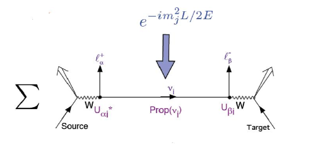
Figure 1: Neutrino flavour change (oscillation) in vacuum

It still remains to be established the value of Prop($\nu_{i}$). To determine it, we’d better study the $\nu_{i}$ in its rest frame. We will label the time in that system $\tau_{i}$. If $\nu_{i}$ does have a rest mass $m_{i}$, then in this frame its state vector satisfies the good old Schrödinger equation

$$i\frac{\partial}{\partial\tau_{i}}|\nu_{i}(\tau_{i})>\;=m_{i}|\nu_{i}(\tau_{i})>\leavevmode\nobreak\ \leavevmode\nobreak\ .$$ (5)

whose solution is given clearly by

$$|\nu_{i}(\tau_{i})>\;=e^{-im_{i}\tau_{i}}|\nu_{i}(0)>\leavevmode\nobreak\ \leavevmode\nobreak\ .$$ (6)

Then, the amplitude for the mass eigenstate $\nu_{i}$ to propagate for a time $\tau_{i}$, is simply the amplitude $<\nu_{i}(0)|\nu_{i}(\tau_{i})>$ for observing the original $\nu_{i}$ $|\nu_{i}(0)>$ after some time as the evoluted state $|\nu_{i}(\tau_{i})>$, i.e. $\exp[-im_{i}\tau_{i}]$. Thus Prop($\nu_{i}$) is only this amplitude where we have used that the time taken by $\nu_{i}$ to travel from the neutrino source to the detector is $\tau_{i}$, the proper time.

Nevertheless, if we want Prop($\nu_{i}$) to be of any use to us, we must write it first in terms of variables in the laboratory system. The natural choice is obviously the laboratory-frame distance, $L$, that the neutrino covers between the source and the detector, and the laboratory-frame time, $t$, that slips away during the journey. The distance $L$ is set by the experimentalists through the selection of the place of settlement of the source and that of the detector. Likewise, the value of the time $t$ is selected by the experimentalists through their election for the time at which the neutrino is created and that when it is detected. Thus, $L$ and $t$ are chosen (hopefully carefully) by the experiment design, and are the same for all the $\nu_{i}$ components of the beam. Different $\nu_{i}$ do travel through an identical distance $L$, in an identical time $t$.

We still need two other laboratory-frame variables, they are the laboratory-frame energy $E_{i}$ and momentum $p_{i}$ of the neutrino mass eigenstate $\nu_{i}$. With the four lab-frame variable and using Lorentz invariance, we can obtain the phase $m_{i}\tau_{i}$ in the $\nu_{i}$ propagator Prop($\nu_{i}$) we have been looking for, which (expressed in terms of laboratory frame variables) is given by

$$m_{i}\tau_{i}=E_{i}t-p_{i}L\leavevmode\nobreak\ \leavevmode\nobreak\ .$$ (7)

At this point however one may argue that, in real life, neutrino sources are basically constant in time, and that the time $t$ that slips away since the neutrino is produced till it dies in the detector is actually not measured. This argument is right. In real life, an experiment averages over the time $t$ used by the neutrino to complete its journey. However, lets consider that two constituents of the neutrino beam, the first one with energy $E_{1}$ and the second one with energy $E_{2}$ (both measured in the lab frame), contribute coherently to the neutrino signal produced in the detector. Now, if we call $t$ to the the time used by the neutrino to cover the distance separating the production and detection points, then by the time the constituent whose energy is $E_{j}\;(j=1,2)$ arrives to the detector, it has raised a phase factor $\exp[-iE_{j}t]$. Therefore, we will have an interference between the $E_{1}$ and $E_{2}$ beam participants that will include a phase factor $\exp[-i(E_{1}-E_{2})t]$. When averaged over the non-observed travel time $t$, this factor goes away, except when $E_{2}=E_{1}$. Therefore, only components of the neutrino beam that share the same energy contribute coherently to the neutrino oscillation signal [2, 3]. Specifically, only the different mass eigenstate constituents of a beam that have the same energy contribute coherently to the oscillation signal.

A mass eigenstate $\nu_{i}$, with mass $m_{i}$, and energy $E$, has a momentum $p_{i}$ given by

$$p_{i}=\sqrt{E^{2}-m_{i}^{2}}\cong E-\frac{m_{i}^{2}}{2E}\leavevmode\nobreak\ \leavevmode\nobreak\ .$$ (8)

Where, we have used that as the masses of the neutrinos are miserably small, $m_{i}^{2}\ll E^{2}$ for any energy $E$ attainable at a realistic experiment. From Eqs. (7) and (8), we see that at energy $E$ the phase $m_{i}\tau_{i}$ appearing in Prop($\nu_{i}$) takes the value

$$m_{i}\tau_{i}\cong E(t-L)+\frac{m_{i}^{2}}{2E}L\leavevmode\nobreak\ \leavevmode\nobreak\ .$$ (9)

As the phase $E(t-L)$ appears in all the interfering terms it will eventually disappear when calculating the transition amplitude. Thus, we can get rid of it already now and use

$$\mathrm{Prop}(\nu_{i})=\exp[-im_{i}^{2}\frac{L}{2E}]\leavevmode\nobreak\ \leavevmode\nobreak\ .$$ (10)

Applying this result, we can obtain from Eq. (4) that the amplitude for a neutrino born as a $\nu_{\alpha}$ to be detected as a $\nu_{\beta}$ after covering a distance $L$ through vacuum with energy $E$ yields

$$\mathrm{Amp}(\nu_{\alpha}\longrightarrow\nu_{\beta})=\sum_{i}U_{\alpha i}^{*}\,e^{-im_{i}^{2}\frac{L}{2E}}U_{\beta i}\leavevmode\nobreak\ \leavevmode\nobreak\ .$$ (11)

The expression above is valid for an arbitrary number of neutrino flavours and mass eigenstates. The probability P($\nu_{\alpha}\longrightarrow\nu_{\beta}$) for $\nu_{\alpha}\longrightarrow\nu_{\beta}$ can be found by squaring it, giving

$$\mathrm{P}(\nu_{\alpha}\longrightarrow\nu_{\beta}) = |\mathrm{Amp}(\nu_{\alpha}\longrightarrow\nu_{\beta})|^{2}$$ (12)

$$= \delta_{\alpha\beta}-4\sum_{i>j}\Re(U^{*}_{\alpha i}U_{\beta i}U_{\alpha j}U^{*}_{\beta j})\sin^{2}\left(\Delta m^{2}_{ij}\frac{L}{4E}\right)$$

$$\phantom{\delta_{\alpha\beta}}+2\sum_{i>j}\Im(U^{*}_{\alpha i}U_{\beta i}U_{\alpha j}U^{*}_{\beta j})\sin\,\left(\Delta m^{2}_{ij}\frac{L}{2E}\right)\leavevmode\nobreak\ \leavevmode\nobreak\ ,$$

with

$$\Delta m_{ij}^{2}\equiv m_{i}^{2}-m_{j}^{2}\leavevmode\nobreak\ \leavevmode\nobreak\ .$$ (13)

In order to get Eq. (12) we have used that the mixing matrix $U$ is unitary.

The oscillation probability P($\nu_{\alpha}\longrightarrow\nu_{\beta}$) we have just obtained corresponds to that of a neutrino, and not to an antineutrino, as we have used that the oscillating neutrino was produced along with a charged antilepton $\bar{\ell}$, and gives birth to a charged lepton $\ell$ once it reaches the detector. The corresponding probability P($\overline{\nu_{\alpha}}\longrightarrow\overline{\nu_{\beta}}$) for an antineutrino oscillation can be obtained from P($\nu_{\alpha}\longrightarrow\nu_{\beta}$) taking advantage of the fact that the two transitions $\overline{\nu_{\alpha}}\longrightarrow\overline{\nu_{\beta}}$ and $\nu_{\beta}\longrightarrow\nu_{\alpha}$ are CPT conjugated processes. Thus, assuming that neutrino interactions respect CPT[4],

$$\mathrm{P}(\overline{\nu_{\alpha}}\longrightarrow\overline{\nu_{\beta}})=\mathrm{P}(\nu_{\beta}\longrightarrow\nu_{\alpha})\leavevmode\nobreak\ \leavevmode\nobreak\ .$$ (14)

Then, from Eq. (12) we obtain that

$$\mathrm{P}(\nu_{\beta}\longrightarrow\nu_{\alpha};\>U)=\mathrm{P}(\nu_{\alpha}\longrightarrow\nu_{\beta};\>U^{*})\leavevmode\nobreak\ \leavevmode\nobreak\ .$$ (15)

Therefore, if CPT is a good symmetry (with respect to neutrino interactions), Eq. (12) tells us that

$$\mathrm{P}(\shortstack{{\tiny(\rule[0.86108pt]{5.0pt}{0.28453pt})} \\ [-.7ex] $\nu_{\alpha}$}\longrightarrow\shortstack{{\tiny(\rule[0.86108pt]{5.0pt}{0.28453pt})} \\ [-.7ex] $\nu_{\beta}$}) = \delta_{\alpha\beta}-4\sum_{i>j}\Re(U^{*}_{\alpha i}U_{\beta i}U_{\alpha j}U^{*}_{\beta j})\sin^{2}\left(\Delta m^{2}_{ij}\frac{L}{4E}\right)$$ (16)

$$\phantom{\delta_{\alpha\beta}}{\rm\raise 3.44444pt\hbox{+}\kern-8.99994pt\lower 2.58334pt\hbox{{\tiny(}--{\tiny)}}}\;2\sum_{i>j}\Im(U^{*}_{\alpha i}U_{\beta i}U_{\alpha j}U^{*}_{\beta j})\sin\,\left(\Delta m^{2}_{ij}\frac{L}{2E}\right)\leavevmode\nobreak\ \leavevmode\nobreak\ .$$

These expressions make it clear that if the mixing matrix $U$ is complex, P($\overline{\nu_{\alpha}}\longrightarrow\overline{\nu_{\beta}}$) and P($\nu_{\alpha}\longrightarrow\nu_{\beta}$) will not be identical, in general. As $\overline{\nu_{\alpha}}\longrightarrow\overline{\nu_{\beta}}$ and $\nu_{\alpha}\longrightarrow\nu_{\beta}$ are CP conjugated processes, P$(\overline{\nu_{\alpha}}\longrightarrow\overline{\nu_{\beta}})\neq\mathrm{P}(\nu_{\alpha}\longrightarrow\nu_{\beta})$ would be an evidence of CP violation in neutrino oscillations. So far, CP violation has been observed only in the quark sector, so its measurement in neutrino oscillations would be quite exciting.

So far, we have been working in natural units, if we return now the $\hbar$’s and $c$ factor (we have happily left out) into the oscillation probability we find that

$$\sin^{2}\left(\Delta m^{2}_{ij}\frac{L}{4E}\right)\;\;\longrightarrow\;\;\sin^{2}\left(\Delta m^{2}_{ij}c^{4}\frac{L}{4\hbar cE}\right)$$ (17)

Having done that, it is easy and instructive to explore the semi-classical limit, $\hbar\longrightarrow 0$. In this limit the oscillation length goes to zero (the oscillation phase goes to infinity) and the oscillations are averaged out. The same happens if we let the mass difference $\Delta m^{2}$ become large. This is exactly what happens in the quark sector (and the reason why we never study quark oscillations despite knowing that mass eigenstates do not coincide with flavour eigenstates).

In terms of real life units (which are not "natural" units), the oscillation phase is given by

$$\Delta m^{2}_{ij}\frac{L}{4E}=1.27\,\Delta m^{2}_{ij}(\mathrm{eV}^{2})\frac{L\,(\mathrm{km})}{E\,(\mathrm{GeV})}\leavevmode\nobreak\ \leavevmode\nobreak\ .$$ (18)

then, since $\sin^{2}[1.27\,\Delta m^{2}_{ij}(\mathrm{eV}^{2})L\,(\mathrm{km})/E\,(\mathrm{GeV})]$ can be experimentally observed only if its argument is of order unity or larger, an experimental set-up with a baseline $L$ (km) and an energy $E$ (GeV) is sensitive to neutrino mass squared differences $\Delta m^{2}_{ij}(\mathrm{eV}^{2})$ larger that or equal to $\sim[L\,(\mathrm{km})/E\,(\mathrm{GeV}]^{-1}$. For example, an experiment with $L\sim 10^{4}$ km, roughly the size of Earth’s diameter, and $E\sim 1$ GeV is sensitive to $\Delta m^{2}_{ij}$ down to $\sim\!10^{-4}$ eV². This fact makes it clear that neutrino oscillation experiments can test super tiny neutrino masses. It does so by exhibiting quantum mechanical interferences between amplitudes whose relative phases are proportional to these super tiny neutrino mass squared differences, which can be transformed into sizeable effects by choosing an $L/E$ large enough.

But let’s keep analysing the oscillation probability and see whether we can learn more about neutrino oscillations by studying its expression.

It is clear from $\mathrm{P}(\shortstack{{\tiny(\rule[0.86108pt]{5.0pt}{0.28453pt})} \\ [-.7ex] $\nu_{\alpha}$}\longrightarrow\shortstack{{\tiny(\rule[0.86108pt]{5.0pt}{0.28453pt})} \\ [-.7ex] $\nu_{\beta}$})$ that if neutrinos have zero mass, in such a way that all $\Delta m^{2}_{ij}=0$, then, $\mathrm{P}(\shortstack{{\tiny(\rule[0.86108pt]{5.0pt}{0.28453pt})} \\ [-.7ex] $\nu_{\alpha}$}\longrightarrow\shortstack{{\tiny(\rule[0.86108pt]{5.0pt}{0.28453pt})} \\ [-.7ex] $\nu_{\beta}$})=\delta_{\alpha\beta}$. Therefore, the experimental observation that neutrinos can morph from one flavour to a different one indicates that neutrinos are not only massive but also that their masses are not degenerate. Actually, it was precisely this evidence the one that led to the conclusion that neutrinos are massive.

However, every neutrino oscillation seen so far has involved at some point neutrinos that travel through matter. But the expression we derived is valid only for flavour change in vacuum, and does not take into account any interaction between the neutrinos and the matter traversed between their source and their detector. Thus, one might ask whether flavour-changing interactions between neutrinos and matter are indeed responsible of the observed flavour changes, and not neutrino masses. Regarding this question, two points can be made. First, although it is true that the Standard Model of elementary particle physics contains only mass-less neutrinos, it provides an amazingly well corroborated description of neutrino interactions, and this description clearly establishes that neutrino interactions with matter do not change flavour. Second, for at least some of the observed flavour changes, matter effects are expected to be miserably small, and there is solid evidence that in these cases, the flavour transition probability depends on $L$ and $E$ through the combination $L/E$, as anticipated by the oscillation hypothesis. Modulo a constant, $L/E$ is precisely the proper time that goes by in the rest frame of the neutrino as it covers a distance $L$ possessing an energy $E$. Thus, these flavour transitions behave as if they were a progression of the neutrino itself over time, rather than a result of interaction with matter.

Now, suppose the leptonic mixings were trivial. This would mean that in the decay $W^{+}\longrightarrow\overline{\ell_{\alpha}}+\nu_{i}$, which as we established has an amplitude $U_{\alpha i}^{*}$, the emerging charged antilepton $\overline{\ell_{\alpha}}$ of flavour $\alpha$ comes along always with the same neutrino mass eigenstate $\nu_{i}$. That is, if $U_{\alpha i}^{*}\neq 0$, then $U_{\alpha j}$ becomes zero for all $j\neq i$. Therefore, from Eq. (16) it is clear that, $\mathrm{P}(\shortstack{{\tiny(\rule[0.86108pt]{5.0pt}{0.28453pt})} \\ [-.7ex] $\nu_{\alpha}$}\longrightarrow\shortstack{{\tiny(\rule[0.86108pt]{5.0pt}{0.28453pt})} \\ [-.7ex] $\nu_{\beta}$})=\delta_{\alpha\beta}$. Thus, the observation that neutrinos can change flavour indicates mixing.

Then, there are basically two ways to detect neutrino flavour change. The first one is to observe, in a beam of neutrinos which are all created of the same flavour, say $\alpha$, some appearance of neutrinos of a new flavour $\beta$ that is different from the flavour $\alpha$ we started with. This is what is called an appearance experiment. The second way is to start with a beam of identical $\nu_{\alpha}$s, whose flux is known, and observe that this known $\nu_{\alpha}$ flux is depleted. This is called a disappearance experiment.

As Eq. (16) shows, the transition probability in vacuum does not only depend on $L/E$ but also oscillates with it. It is because of this fact that neutrino flavour transitions are named “neutrino oscillations”. Now notice also that neutrino transition probabilities depend only on neutrino squared-mass splittings, and not on the individual squared neutrino masses themselves. Thus, oscillation experiments can only measure the neutrino squared-mass spectral pattern, but not its absolute scale, i.e. the distance above zero the entire pattern lies.

It is clear that neutrino transitions cannot modify the total flux in a neutrino beam, but simply alter its distribution between the different flavours. Actually, from Eq. (16) and the unitarity of the $U$ matrix, it follows that

$$\sum_{\beta}\mathrm{P}(\shortstack{{\tiny(\rule[0.86108pt]{5.0pt}{0.28453pt})} \\ [-.7ex] $\nu_{\alpha}$}\longrightarrow\shortstack{{\tiny(\rule[0.86108pt]{5.0pt}{0.28453pt})} \\ [-.7ex] $\nu_{\beta}$})=1\leavevmode\nobreak\ \leavevmode\nobreak\ ,$$ (19)

where the sum runs over all flavours $\beta$, including the original flavour $\alpha$. Eq. (19) makes it transparent that the probability that a neutrino morphs its flavour, added to the probability that it does not do so, is one. Ergo, flavour transitions do not change the total flux. Nevertheless, some of the flavours $\beta\neq\alpha$ into which a neutrino can oscillate into may be sterile flavours; that is, flavours that do not take part in weak interactions and therefore escape detection. If any of the original (active) neutrino flux turns into sterile, then an experiment measuring the total active neutrino flux—that is, the sum of the $\nu_{e},\;\nu_{\mu}$, and $\nu_{\tau}$ fluxes—will find it to be less than the original flux. In the experiments performed up today, no flux was ever missed.

In the literature, description of neutrino oscillation normally assume that the different mass eigenstates $\nu_{i}$ that contribute coherently to a beam share the same momentum, rather than the same energy as we have argued they must have. While the supposition of equal momentum is technically wrong, it is an inoffensive mistake, since, as can easily be shown [5], it conveys to the same oscillation probabilities as we have found.

A relevant and interesting case of the (not that simple) formula for P$(\overline{\nu_{\alpha}}\longrightarrow\overline{\nu_{\beta}})$ is the case where only two flavours participate in the oscillation. The only-two-neutrino scenario is a rather rigorous description of a vast number of experiments. Lets assume then, that only two mass eigenstates, which we will name $\nu_{1}$ and $\nu_{2}$, and two corresponding flavour states, which we will name $\nu_{\mu}$ and $\nu_{\tau}$, are relevant. There is then only one squared-mass splitting, $m^{2}_{2}-m^{2}_{1}\equiv\Delta m^{2}$. Even more, neglecting phase factors that can be proven to have no effect on oscillation, the mixing matrix $U$ takes the simple form

$$\left(\begin{array}[]{c}\nu_{\mu}\\ \nu_{\tau}\end{array}\right)=\left(\begin{array}[]{cc}\phantom{-}\cos\theta&\sin\theta\\ -\sin\theta&\cos\theta\end{array}\right)\left(\begin{array}[]{c}\nu_{1}\\ \nu_{2}\end{array}\right)$$ (20)

The $U$ of Eq. (20) is just a 2$\times$2 rotation matrix, and the rotation angle $\theta$ within it is referred to as the mixing angle. Inserting the $U$ of Eq. (20) and the unique $\Delta m^{2}$ into the general expression for P$(\overline{\nu_{\alpha}}\longrightarrow\overline{\nu_{\beta}})$, Eq. (16), we immediately find that, for $\beta\neq\alpha$, when only two neutrinos are relevant,

$$\mathrm{P}(\overline{\nu_{\alpha}}\longrightarrow\overline{\nu_{\beta}})=\sin^{2}2\theta\sin^{2}\left(\frac{\Delta m^{2}\;L}{4E}\right)\leavevmode\nobreak\ \leavevmode\nobreak\ .$$ (21)

Moreover, the survival probability, i.e. the probability that the neutrino remains with the same flavour its was created with is, as usual, unity minus the probability that it changes flavour.

0.3 Neutrino oscillations in matter

When we create a beam of neutrinos on earth through an accelerator and send it up to thousand kilometres away to a meet detector, the beam does not move through vacuum, but through matter, earth matter. The beam of neutrinos then scatters (coherently forward) from particles it meets along the way. Such a scattering can have a large effect on the transition probabilities. We will assume that neutrino interactions with matter are flavour conserving, as described by the Standard Model. Then a neutrino in matter have two possibilities to enjoy coherent forward scattering from matter particles . First, if it is an electron neutrino, $\nu_{e}$—and only in this case—can exchange a $W$ boson with an electron. Neutrino-electron coherent forward scattering via $W$ exchange opens up an extra interaction potential energy $V_{W}$ suffered exclusively by electron neutrinos. Obviously, this additional weak interaction energy has to be proportional to $G_{F}$, the Fermi coupling constant. In addition, the interaction energy coming from $\nu_{e}-e$ scattering grows with $N_{e}$, the number of electrons per unit volume. From the Standard Model, we find that

$$V_{W}=+\sqrt{2}\,G_{F}\,N_{e}\leavevmode\nobreak\ \leavevmode\nobreak\ ,$$ (22)

clearly, this interaction energy affects also antineutrinos (in a opposite way though), it changes sign if we replace the $\nu_{e}$ by $\overline{\nu_{e}}$.

The second interaction corresponds to the case where a neutrino in matter exchanges a $Z$ boson with an matter electron, proton, or neutron. The Standard Model teaches us that weak interactions are flavour blind. Every flavour of neutrino enjoys them, and the amplitude for this $Z$ exchange is always the same. It also teaches us that, at zero momentum transfer, the $Z$ couplings to electrons and protons have equal strength and opposite sign. Therefore, counting on the fact that the matter through which our neutrino moves is electrically neutral (it contains equal number of electrons and protons), the electron and proton contribution to coherent forward neutrino scattering through $Z$ exchange will add up to zero. Then, the effect of the $Z$ exchange contribution to the interaction potential energy $V_{Z}$ will be equal to all flavors and will depends exclusively on $N_{n}$, the number density of neutrons. From the Standard Model, we find that

$$V_{Z}=-\frac{\sqrt{2}}{2}\,G_{F}\,N_{n}\leavevmode\nobreak\ \leavevmode\nobreak\ ,$$ (23)

as was the case before, for $V_{W}$, this contribution will flip sign if we replace the neutrinos by anti-neutrinos.

But we already learnt that Standard Model interactions do not change neutrino flavour. Therefore, unless non-Standard-Model flavour changing interactions play a role, neutrino flavour transitions or neutrino oscillations points also to neutrino mass and mixing even when neutrinos are propagating through matter.

Neutrino propagation in matter is easy to understand when analyzed through a time dependent Schrödinger equation in the laboratory frame

$$i\frac{\partial}{\partial t}|\nu(t)>\;=\mathcal{H}|\nu(t)>\leavevmode\nobreak\ \leavevmode\nobreak\ .$$ (24)

where, $|\nu(t)\!>$ is a multicomponent neutrino vector state, in which each neutrino flavour corresponds to one component. In the same way, the Hamiltonian $\mathcal{H}$ is a matrix in flavour space. To make our lives easy, lets analyze the case where only two neutrino flavours are relevant, say $\nu_{e}$ and $\nu_{\mu}$. Then

$$|\nu(t)>\;=\left(\begin{array}[]{c}f_{e}(t)\\ f_{\mu}(t)\end{array}\right)\leavevmode\nobreak\ \leavevmode\nobreak\ ,$$ (25)

where $f_{e}(t)^{2}$ is the fraction of the neutrino that is a $\nu_{e}$ at time $t$, and similarly for $f_{\mu}(t)$. Analogously, $\mathcal{H}$ is a 2$\times$2 matrix in $\nu_{e}-\nu_{\mu}$ space.

It will prove to be clarifying to work out the two flavour case in vacuum first, and add matter effects afterwards. Using Eq. (2) for $|\nu_{\alpha}>$ as a linear combination of mass eigenstates, we can see that the $\nu_{\alpha}-\nu_{\beta}$ matrix element of the Hamiltonian in vacuum, $\mathcal{H}_{\mathrm{Vac}}$, can be written as

$$<\nu_{\alpha}|\mathcal{H}_{\mathrm{Vac}}|\nu_{\beta}> = <\sum_{i}U^{*}_{\alpha i}\nu_{i}|\mathcal{H}_{\mathrm{Vac}}|\sum_{j}U^{*}_{\beta j}\nu_{j}>$$ (26)

$$= \sum_{j}U_{\alpha j}U^{*}_{\beta j}\sqrt{p^{2}+m_{j}^{2}}\leavevmode\nobreak\ \leavevmode\nobreak\ .$$

where we are supposing that neutrino belongs to a beam where all its mass components (the mass eigenstates) share the same definite momentum $p$. (As we have already mentioned, this supposition is technically wrong, however it leads anyway to the right oscillation probability.) In the second line of Eq. (26), we have used that

$$\mathcal{H}_{\mathrm{Vac}}|\nu_{j}>=E_{j}|\nu_{j}>$$ (27)

with $E_{j}=\sqrt{p^{2}+m_{j}^{2}}$ the energy of the mass eigenstate $\nu_{j}$ with momentum $p$, and the fact that the mass eigenstates of the Hermitian Hamiltonian $\mathcal{H}_{\mathrm{Vac}}$ constitute a basis and therefore are orthogonal.

As we have already mentioned, neutrino oscillations are the archetype quantum interference phenomenon, where only the relative phases of the interfering states play a role. Therefore, only the relative energies of these states, which set their relative phases, are relevant. As a consequence, if it proves to be convenient, we can feel free to happily remove from the Hamiltonian $\mathcal{H}$ any contribution proportional to the identity matrix $I$. As we have said, this substraction will leave unaffected the differences between the eigenvalues of $\mathcal{H}$, and therefore will leave unaffected the prediction of $\mathcal{H}$ for flavour transitions.

It goes without saying that as in this case only two neutrinos are relevant, there are only two mass eigenstates, $\nu_{1}$ and $\nu_{2}$, and only one mass splitting $\Delta m^{2}\equiv m^{2}_{2}-m^{2}_{1}$, and therefore the $U$ matrix is given by Eq. (20). Inserting this matrix into Eq. (26), and applying the high momentum approximation $(p^{2}+m^{2}_{j})^{1/2}\cong p+m^{2}_{j}/2p$, and removing from $\mathcal{H}_{\mathrm{Vac}}$ a term proportional to the the identity matrix (a removal we know is going to be harmless), we get

$$\mathcal{H}_{\mathrm{Vac}}=\frac{\Delta m^{2}}{4E}\left(\begin{array}[]{cc}-\cos 2\theta&\sin 2\theta\\ \phantom{-}\sin 2\theta&\cos 2\theta\end{array}\right)\leavevmode\nobreak\ \leavevmode\nobreak\ .$$ (28)

To write this expression, we have used that $p\cong E$, where $E$ is the average energy of the neutrino mass eigenstates in our neutrino beam of ultra high momentum $p$.

It is not difficult to corroborate that the Hamiltonian $\mathcal{H}_{\mathrm{Vac}}$ of Eq. (28) for the two neutrino scenario would give an identical oscillation probability , Eq. (21), as the one we have already obtained in a different way. For example, lets have a look at the oscillation probability for the process $\nu_{e}\longrightarrow\nu_{\mu}$. From Eq. (20) it is clear that in terms of the mixing angle, the electron neutrino state composition is

$$|\nu_{e}>\;=\phantom{-}|\nu_{1}>\cos\theta+|\nu_{2}>\sin\theta\leavevmode\nobreak\ \leavevmode\nobreak\ ,$$ (29)

while that of the muon neutrino is given by

$$|\nu_{\mu}>\;=-|\nu_{1}>\sin\theta+|\nu_{2}>\cos\theta\leavevmode\nobreak\ \leavevmode\nobreak\ .$$ (30)

Now, the eigenvalues of $\mathcal{H}_{\mathrm{Vac}}$, 25, read

$$\lambda_{1}=-\frac{\Delta m^{2}}{4E}\leavevmode\nobreak\ \leavevmode\nobreak\ ,\;\lambda_{2}=+\frac{\Delta m^{2}}{4E}\leavevmode\nobreak\ \leavevmode\nobreak\ .$$ (31)

The eigenvectors of this Hamiltonian, $|\nu_{1}>$ and $|\nu_{2}>$, can also be written in terms of $|\nu_{e}>$ and $|\nu_{\mu}>$ by means of Eqs. (29) and (30). Therefore, with $\mathcal{H}$, its vacuum expression, $\mathcal{H}_{\mathrm{Vac}}$ of Eq. (28), the Schrödinger equation of Eq. (24) tells us that if at time $t=0$ we begin from a $|\nu_{e}>$, then after some time $t$ this $|\nu_{e}>$ will progress into the state

$$|\nu(t)>\;=|\nu_{1}>e^{+i\frac{\Delta m^{2}}{4E}t}\cos\theta+|\nu_{2}>e^{-i\frac{\Delta m^{2}}{4E}t}\sin\theta\leavevmode\nobreak\ \leavevmode\nobreak\ .$$ (32)

Thus, the probability P$(\nu_{e}\longrightarrow\nu_{\mu})$ that this evoluted neutrino be detected as a different flavour $\nu_{\mu}$, from Eqs. (30) and (32), is given by,

$$\mathrm{P}(\nu_{e}\longrightarrow\nu_{\mu}) = |<\nu_{\mu}|\nu(t)>|^{2}$$ (33)

$$= |\sin\theta\cos\theta(-e^{i\frac{\Delta m^{2}}{4E}t}+e^{-i\frac{\Delta m^{2}}{4E}t})|^{2}$$

$$= \sin^{2}2\theta\sin^{2}\left(\Delta m^{2}\frac{L}{4E}\right)\leavevmode\nobreak\ \leavevmode\nobreak\ .$$

Where we have substituted the time $t$ travelled by our highly relativistic state by the distance $L$ it has covered. The flavour transition or oscillation probability of Eq. (33), as expected, is exactly the same we have found before, Eq. (21).

We can now move on to analyze neutrino propagation in matter. In this case, the 2$\times$2 vacuum Hamiltonian $\mathcal{H}_{\mathrm{Vac}}$ receives two additional contributions and becomes $\mathcal{H}_{M}$, which is given by

$$\mathcal{H}_{M}=\mathcal{H}_{\mathrm{Vac}}+V_{W}\left(\begin{array}[]{cc}1&0\\ 0&0\end{array}\right)+V_{Z}\left(\begin{array}[]{cc}1&0\\ 0&1\end{array}\right)\leavevmode\nobreak\ \leavevmode\nobreak\ .$$ (34)

In the new Hamiltonian, the first additional contribution corresponds to the interaction potential due to $W$ exchange, Eq. (22). As this interaction is suffered only by $\nu_{e}$, this contribution is different from zero only in the upper left, $\nu_{e}-\nu_{e}$, element of $\mathcal{H}_{M}$. The second additional contribution, the last term of Eq. (34) comes from the interaction potential due to $Z$ exchange, Eq. (23). Since this interaction is flavour blind, it affects every neutrino flavour in the same way, its contribution to $\mathcal{H}_{M}$ is proportional to the identity matrix, and can be safely neglected. Then

$$\mathcal{H}_{M}=\mathcal{H}_{\mathrm{Vac}}+\frac{V_{W}}{2}+\frac{V_{W}}{2}\left(\begin{array}[]{cc}1&0\\ 0&-1\end{array}\right)\leavevmode\nobreak\ \leavevmode\nobreak\ ,$$ (35)

where (for reasons that are going to become clear later) we have divided the $W$-exchange contribution into two pieces, one a multiple of the identity matrix (that we will disregard in the next step) and, a piece that it is not a multiple of the identity matrix. Disregarding the first piece as promised, we have from Eqs. (28) and (35)

$$\mathcal{H}_{M}=\frac{\Delta m^{2}}{4E}\left(\begin{array}[]{cc}-(\cos 2\theta-A)&\sin 2\theta\\ \sin 2\theta&(\cos 2\theta-A)\end{array}\right)\leavevmode\nobreak\ \leavevmode\nobreak\ ,$$ (36)

where

$$A\equiv\frac{V_{W}/2}{\Delta m^{2}/4E}=\frac{2\sqrt{2}G_{F}N_{e}E}{\Delta m^{2}}\leavevmode\nobreak\ \leavevmode\nobreak\ .$$ (37)

Clearly, $A$ shows the size (the importance) of the matter effects as compared to the neutrino squared-mass splitting and signal the situations when they become important.

Now, if we define

$$\Delta m^{2}_{M}\equiv\Delta m^{2}\sqrt{\sin^{2}2\theta+(\cos 2\theta-A)^{2}}$$ (38)

and

$$\sin^{2}2\theta^{M}\equiv\frac{\sin^{2}2\theta}{\sin^{2}2\theta+(\cos 2\theta-A)^{2}}\leavevmode\nobreak\ \leavevmode\nobreak\ ,$$ (39)

$\mathcal{H}_{M}$ can be given as

$$\mathcal{H}_{M}=\frac{\Delta m^{2}_{M}}{4E}\left(\begin{array}[]{cc}-\cos 2\theta^{M}&\sin 2\theta^{M}\\ \phantom{-}\sin 2\theta^{M}&\cos 2\theta^{M}\end{array}\right)\leavevmode\nobreak\ \leavevmode\nobreak\ .$$ (40)

That is, the Hamiltonian in matter, $\mathcal{H}_{M}$, becomes formally identical to its vacuum counterpart, $\mathcal{H}_{\mathrm{Vac}}$, Eq. (28), except that the vacuum parameters $\Delta m^{2}$ and $\theta$ are now given by the matter ones, $\Delta m^{2}_{M}$ and $\theta^{M}$, respectively.

Obviously, the eigenstates of $\mathcal{H}_{M}$ are not identical to their vacuum counterparts. The splitting between the squared masses of the matter eigenstates is not the same as the vacuum splitting $\Delta m^{2}$, and the same happens with the mixing angle, the mixing in matter—the angle that rotates from the $\nu_{e},\nu_{\mu}$ basis, to the mass basis—is different from the vacuum mixing angle $\theta$. Clearly however, all the physics of neutrino propagation in matter is controlled by the matter Hamiltonian $\mathcal{H}_{M}$. However, according to Eq. (40), at least at the formal level, $\mathcal{H}_{M}$ has the same functional dependence on the matter parameters $\Delta m^{2}_{M}$ and $\theta^{M}$ in as the vacuum Hamiltonian $\mathcal{H}_{\mathrm{Vac}}$, Eq. (28), on the vacuum ones, $\Delta m^{2}$ and $\theta$. Therefore, $\Delta m^{2}_{M}$ corresponds to the effective splitting between the squared masses of the eigenstates in matter, and $\theta^{M}$ corresponds to the effective mixing angle in matter.

In a typical experimental set-up where the neutrino beam is generated by an accelerator and sent away to a detector that is, say, several hundred, or even thousand kilometers away, it traverses through earth matter, but only superficially , it does not get deep into the earth. The matter density met by such a beam en voyage can be taken to be approximately constant. Therefore, the electron density $N_{e}$ is also constant, and the same happens with the parameter $A$, and the matter Hamiltonian $\mathcal{H}_{M}$. They all become approximately position independent, and therefore quite analogue to the vacuum Hamiltonian $\mathcal{H}_{\mathrm{Vac}}$, which was absolutely position independent. Comparing Eqs. (40) and (28), we can immediately conclude that since $\mathcal{H}_{\mathrm{Vac}}$ gives rise to the vacuum oscillation probability P$(\nu_{e}\longrightarrow\nu_{\mu})$ of Eq. (33), $\mathcal{H}_{M}$ must give rise to a matter oscillation probability of the form

$$\mathrm{P}_{M}(\nu_{e}\longrightarrow\nu_{\mu})=\sin^{2}2\theta^{M}\sin^{2}\left(\Delta m^{2}_{M}\frac{L}{4E}\right)\leavevmode\nobreak\ \leavevmode\nobreak\ .$$ (41)

That is, the oscillation probability in matter (formally) is the same as in vacuum, except that the vacuum parameters $\theta$ and $\Delta m^{2}$ are replaced by their matter counterparts.

In theory, judging simply its potential, matter effects can have very drastic effects. From Eq. (39) for the effective mixing angle in matter, $\theta^{M}$, we can appreciate that even when the vacuum mixing angle $\theta$ is incredible small, say, $\sin^{2}2\theta=10^{-4}$, if we get to have $A\cong\cos 2\theta$, then $\sin^{2}2\theta^{M}$ can be brutally enhanced as compared to its vacuum value and can even reach its maximum possible value, one. This brutal enhancement of a tiny mixing angle in vacuum up to a sizeable one in matter is the “resonant” version of the Mikheyev-Smirnov-Wolfenstein effect [6, 7, 8, 9]. In the beginning of solar neutrino experiments, people entertained the idea that this brutal enhancement was actually taking place inside the sun. Nonetheless, as we will see soon the solar neutrino mixing angle is quite sizeable ($\sim 34^{\circ}$) already in vacuum [10]. Then, although matter effects on the sun are important and they do enhance the solar mixing angle, unfortunately they are not as drastic as we once dreamt.

0.4 Evidence for neutrino oscillations

0.4.1 Atmospheric and accelerator neutrinos

Almost fifteen year have elapsed since we were presented convincing evidence of neutrino masses and mixings, and since then, the evidence has only grown. SuperKamiokande (SK) was the first experiment to present compelling evidence of $\nu_{\mu}$ disappearance in their atmospheric neutrino fluxes, see [12] . In Fig. 2 the zenith angle (the angle subtended with the horizontal) dependence of the multi-GeV $\nu_{\mu}$ sample is shown together with the disappearance as a function of $L/E$ plot. These data fit amazingly well the naive two component neutrino hypothesis with

$$\Delta m^{2}_{\mbox{atm}}=2-3\times 10^{-3}{\mbox{eV}}^{2}\;\;\;{\mbox{and}}\;\;\;\sin^{2}\theta_{\mbox{atm}}=0.50\pm 0.15$$ (42)

Roughly speaking SK corresponds to an $L/E$ for oscillations of 500 km/GeV and almost maximal mixing (the mass eigenstates are nearly even admixtures of muon and tau neutrinos). No signal of an involvement of the third flavour, $\nu_{e}$ is found so the assumption is that atmospheric neutrino disappearance is basically $\nu_{\mu}\longrightarrow\nu_{\tau}$.

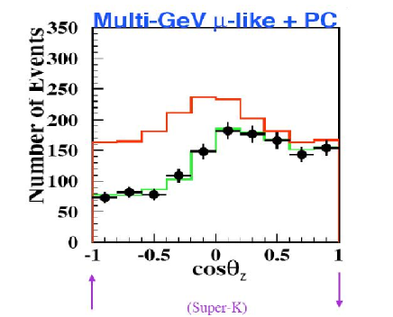
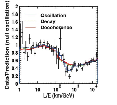
Figure 2: Superkamiokande’s evidence for neutrino oscillations both in the zenith angle and L/E plots

After atmospheric neutrino oscillations were established, two new experiments were built, sending (man-made) beams of $\nu_{\mu}$ neutrinos to detectors located at large distances: the K2K experiment [13, 14], sends neutrinos from the KEK accelerator complex to the old SK mine, with a baseline of 120 km while the MINOS experiment [15], sends its beam from Fermilab, near Chicago, to the Soudan mine in Minnesota, a baseline of 735 km. Both experiments have seen evidence for $\nu_{\mu}$ disappearance consistent with the one found by SK. The results of both are summarised in Fig. 3.

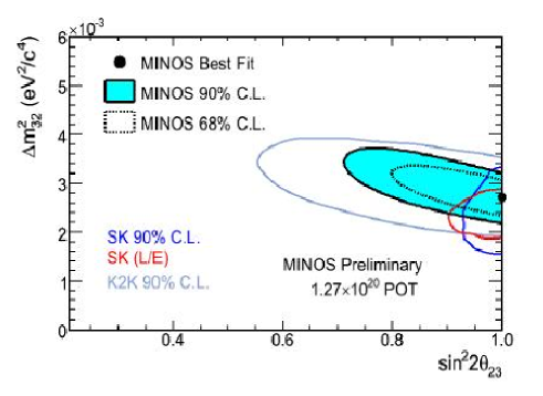
Figure 3: Allowed regions in the $\Delta m^{2}_{\mbox{atm}}$ vs $\sin^{2}\theta_{\mbox{atm}}$ plane for MINOS data as well as for K2K data and two of the SK analyses. MINOS’s best fit point is at $\sin^{2}\theta_{\mbox{atm}}=1$ and $\Delta m^{2}_{\mbox{atm}}=2.7\times 10^{-3}{\mbox{eV}}^{2}$.

0.4.2 Reactor and solar neutrinos

The KamLAND reactor experiment, an antineutrino disappearance experiment, receiving neutrinos from sixteen different reactors, at distances ranging from hundred to thousand kilometers, with an average baseline of 180 km and neutrinos of a few ev, [16, 17], has seen evidence of neutrino oscillations . Such evidence was collected not only at a different $L/E$ than the atmospheric and accelerator experiments but also consists on oscillations involving electron neutrinos, $\nu_{e}$, the ones which were not involved before. These oscillations have also been seen for neutrinos coming from the sun (the sun produces only electron neutrinos). However,in order to compare the two experiments we should assume that neutrinos (solar) and antineutrinos (reactor) behave in the same way, i.e. assume CPT conservation. The best fit values in the two neutrino scenario for the KamLAND experiment are

$$\Delta m^{2}_{\odot}=8.0\pm 0.4\times 10^{-5}\mbox{eV}^{2}\;\;\;\mbox{and}\;\;\;\sin^{2}\theta_{\odot}=0.31\pm 0.03$$ (43)

In this case, the $L/E$ involved is 15 km/MeV which is more than an order of magnitude larger than the atmospheric scale and the mixing angle, although large, is clearly not maximal.

Fig. 4 shows the disappearance probability for the $\bar{\nu}_{e}$ for KamLAND as well as several older reactor experiments with shorter baselines.The second panel depicts the flavour content of the ⁸Boron solar neutrino flux (with GeV energies) measured by SNO, [18], and SK, [19]. The reactor outcome can be explained in terms of two flavour oscillations in vacuum, given that the fit to the disappearance probability, is appropriately averaged over $E$ and $L$.

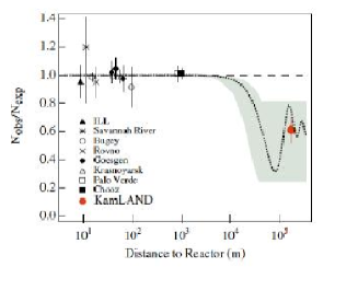
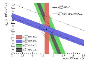
Figure 4: Disappearance of the $\bar{\nu}_{e}$ observed by reactor experiments as a function of distance from the reactor. The flavour content of the ⁸Boron solar neutrinos for the various reactions for SNO and SK. CC: $\nu_{e}+d\longrightarrow e^{-}+p+p$, NC:$\nu_{x}+d\longrightarrow\nu_{x}+p+n$ and ES: $\nu_{\alpha}+e^{-}\longrightarrow\nu_{\alpha}+e^{-}$.

The analysis of neutrinos coming from the sun is slightly more sophisticated because it should include the matter effects that the neutrinos suffer since they are born (at the centre of the sun) until they leave it, which are important at least for the ⁸Boron neutrinos. The pp and ⁷Be neutrinos are less energetic and therefore are not significantly altered by the presence of matter and leave the sun as if it where ethereal. ⁸Boron neutrinos on the other hand, leave the sun strongly affected by the presence of matter and this is evidenced by the fact that they leave the sun as the $\nu_{2}$ mass eigenstate and therefore do not undergo oscillations. This difference is, as mentioned, due mainly to their differences at birth. While pp (⁷Be) neutrinos are created with an average energy of 0.2 MeV (0.9 MeV), ⁸B are born with 10 MeV and as we have seen the impact of matter effects grows with the energy of the neutrino.

However, we should stress that we do not really see solar neutrino oscillations. To trace the oscillation pattern, we need a kinematic phase of order one. In the case of neutrinos coming from the sun the kinematic phase is

$$\Delta_{\odot}=\frac{\Delta m^{2}_{\odot}L}{4E}=10^{7\pm 1}.$$ (44)

Therefore, solar neutrinos behave as "effectively incoherent" mass eigenstates once they leave the sun, and remains being so once they reach the earth. Consequently the $\nu_{e}$ survival probability is given by

$$\langle P_{ee}\rangle=f_{1}\cos^{2}\theta_{\odot}+f_{2}\sin^{2}\theta_{\odot}$$ (45)

where $f_{1}$ is the $\nu_{1}$ content or fraction of $\nu_{\mu}$ and $f_{2}$ is the $\nu_{2}$ content of $\nu_{\mu}$ and therefore both fractions satisfy

$$f_{1}+f_{2}=1.$$ (46)

However, as we have mentioned, pp and ⁷Be solar neutrinos are not affected by the solar matter and oscillate as in vacuum and thus, in their case $f_{1}\approx\cos^{2}\theta_{\odot}=0.69$ and $f_{2}\approx\sin^{2}\theta_{\odot}=0.31$. In the ⁸B a neutrino case, however, matter effects are important and the corresponding fractions are substantially altered, see Fig. 5.

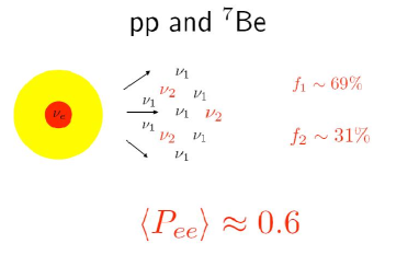
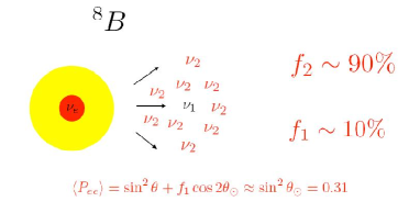
Figure 5: The sun produces $\nu_{e}$ in the core but once they exit the sun thinking about them in the mass eigenstate basis is useful. The fraction of $\nu_{1}$ and $\nu_{2}$ is energy dependent above 1 MeV and has a dramatic effect on the ⁸Boron solar neutrinos, as first observed by Davis.

In a two neutrino scenario, the day-time CC/NC measured by SNO, which is roughly identical to the day-time average $\nu_{e}$ survival probability, $\langle P_{ee}\rangle$, reads

$$\left.\frac{CC}{NC}\right|_{\mbox{day}}=\langle P_{ee}\rangle=f_{1}\cos^{2}\theta_{\odot}+f_{2}\sin^{2}\theta_{\odot},$$ (47)

where $f_{1}$ and $f_{2}=1-f_{1}$ are the $\nu_{1}$ and $\nu_{2}$ contents of the muon neutrino, respectively, averaged over the ⁸B neutrino energy spectrum appropriately weighted with the charged current current cross section. Therefore, the $\nu_{1}$ fraction (or how much $f_{2}$ differs from 100% ) is given by

$$f_{1}=\frac{\left(\left.\frac{CC}{NC}\right|_{\mbox{day}}-\sin^{2}\theta_{\odot}\right)}{\cos 2\theta_{\odot}}=\frac{\left(0.347-0.311\right)}{0.378}\approx 10\%$$ (48)

where the central values of the last SNO analysis, [18], were used. As there are strong correlations between the uncertainties of the CC/NC ratio and $\sin^{2}\theta_{\odot}$ it is not obvious how to estimate the uncertainty on $f_{1}$ from their analysis. Note, that if the fraction of $\nu_{2}$ were 100%, then $\left.\frac{CC}{NC}\right|_{\mbox{day}}=\sin^{2}\theta_{\odot}$.

Using the analytical analysis of the Mikheyev-Smirnov-Wolfenstein (MSW) effect, provided in [20], one can obtain the mass eigenstate fractions, which are given by

$$f_{2}=1-f_{1}=\langle\sin^{2}\theta_{\odot}^{M}+P_{x}\cos 2\theta_{\odot}^{M}\rangle_{{}^{8}{\mbox{B}}},$$ (49)

with $\theta_{\odot}^{M}$ being the mixing angle as given at the $\nu_{e}$ production point and $P_{x}$ is the probability of the neutrino to hop from one mass eigenstate to the second one during the Mikheyev-Smirnov resonance crossing. The average $\langle...\rangle_{{}^{8}{\mbox{B}}}$ is over the electron density of the ⁸B $\nu_{e}$ production region in the centre of the Sun as given by the Solar Standard Model and the energy spectrum of ⁸B neutrinos appropriately weighted with SNO’s charged current cross section. All in all, the ⁸B energy weighted average content of $\nu_{2}$’s measured by SNO is

$$f_{2}=91\pm 2\%{\mbox{ at the 95 \% C.L.}}$$ (50)

Therefore, it is obvious that the ⁸B solar neutrinos are the purest mass eigenstate neutrino beam known so far and SK super famous picture of the sun taken (underground) with neutrinos is made with approximately 90% of $\nu_{2}$ .

On March 8, 2012 a newly built reactor neutrino experiment, the Daya Bay experiment, located in China, announced the measurement of the third mixing angle [11], the only one which was still missing and found it to be

$$\sin^{2}(2\theta_{12})=0.092\pm 0.017\;$$ (51)

The fact that this angle, although smaller that the other two, is still sizeable opens the door to a new generation of neutrino experiments aiming to answer the open questions in the field.

0.5 $\nu$ Standard Model

Now that we have understood the physics behind neutrinos oscillations and have learnt the experimental evidence about the parameters driving this oscillations, we can move ahead and construct the Neutrino Standard Model:

• it consists of three light ($m_{i}$ $<$ 1 eV) neutrinos, i.e. it involves only two mass differences

  $\Delta m^{2}_{\mbox{atm}}\approx 2.5\times 10^{-3}\mbox{eV}^{2}$ and $\Delta m^{2}_{\mbox{solar}}\approx 8.0\times 10^{-5}{\mbox{eV}}^{2}$ .

• so far we have not seen any experimental indication (or need) for additional neutrinos. As we have measured long time ago the invisible width of the $Z$ boson and found it to be 3, if new neutrinos are going to be incorporated into the model, they cannot couple to the $Z$ boson, they cannot enjoy weak interactions, so we call them sterile. However, as sterile neutrinos have not been seen, and are not needed, our Neutrino Standard Model will contain only the three active flavours: $e$, $\mu$ and $\tau$.

  

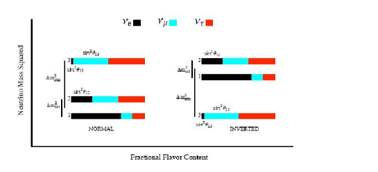
  Figure 6: Flavour content of the three neutrino mass eigenstates (not including the dependence on the cosine of the CP violating phase $\delta$).If CPT is conserved, the flavour content must be the same for neutrinos and anti-neutrinos. Notice that oscillation experiments cannot tell us how far above zero the entire spectrum lies.

• the unitary mixing matrix, called the PMNS matrix, which describes the relation between flavour eigenstates and mass eigenstates, comprises three mixing angles (the so called solar mixing angle:$\theta_{12}$, the atmospheric mixing angle $\theta_{23}$, and the recently measured reactor mixing angle$\theta_{13}$) , one Dirac phase ($\delta$) and possibly two Majorana phases ($\alpha$, $\beta$) and is given by

  $$\mid\nu_{\alpha}\rangle=U_{\alpha i}\mid\nu_{i}\rangle$$

  $$U_{\alpha i}=\left(\begin{array}[]{ccc}1&&\\ &c_{23}&s_{23}\\ &-s_{23}&c_{23}\end{array}\right)\left(\begin{array}[]{ccc}c_{13}&&s_{13}e^{-i\delta}\\ &1&\\ -s_{13}e^{i\delta}&&c_{13}\end{array}\right)\left(\begin{array}[]{ccc}c_{12}&s_{12}&\\ -s_{12}&c_{12}&\\ &&1\end{array}\right)\left(\begin{array}[]{ccc}1&&\\ &e^{i\alpha}&\\ &&e^{i\beta}\end{array}\right)$$ (64)

  where $s_{ij}=\sin\theta_{ij}$ and $c_{ij}=\cos\theta_{ij}$. Thanks to the hierarchy in mass differences (and to a less extent the smallness of the reactor mixing angle) we are allowed to identify the (23) label in the three neutrino scenario with the atmospheric $\delta m^{2}_{\mbox{atm}}$ we obtained in the two neutrino scenario, identically the (12) label can be assimilated to the solar $\delta m^{2}_{\odot}$. The (13) sector drives the $\nu_{e}$ flavour oscillations at the atmospheric scale, and the depletion in reactor neutrino fluxes see [21]. Therefore,

  $$\sin^{2}\theta_{12}=0.31\pm 0.03\;\;\;;\;\;\;\sin^{2}\theta_{23})=0.50\pm 0.15\;\;\;;\;\;\;\sin^{2}\theta_{13}=0.15\pm 0.03$$

  and the mass splittings are

  $$\mid\Delta m^{2}_{32}\mid=2.7\pm 0.4\times 10^{-3}{\mbox{eV}}^{2}\;\;\;{\mbox{and}}\;\;\;\Delta m^{2}_{21}=+8.0\pm 0.4\times 10^{-5}{\mbox{eV}}^{2}.$$

  These mixing angles and mass splittings are summarised in Fig. 6.

• The absolute mass scale of the neutrinos, or the mass of the lightest neutrino is not know yet, but the heaviest one must be lighter than about .5 eV.

• As transition or survival probabilities depend on the combination $U^{*}_{\alpha i}U_{\beta i}$ no trace of the Majorana phases could appear on oscillation phenomena, however they can have observable effects in those processes where the Majorana character of the neutrino is essential for the process to happen, like neutrino-less double beta decay.

0.6 Neutrino mass and character

0.6.1 Absolute neutrino mass

The absolute mass scale of the neutrino cannot be obtained in oscillation experiments, however this does not mean we cannot have it. Direct experiments like tritium beta decay, or neutrinoless double beta decay and indirect ones, like cosmological observations, have potential to feed us the information on the absolute scale of neutrino mass, we so desperately need. The Katrin tritium beta decay experiment, [22], has sensitivity down to 200 meV for the "mass" of $\nu_{e}$ defined as

$$m_{\nu_{e}}=\mid U_{e1}\mid^{2}m_{1}+\mid U_{e2}\mid^{2}m_{2}+\mid U_{e3}\mid^{2}m_{3}.$$ (65)

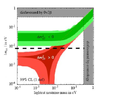
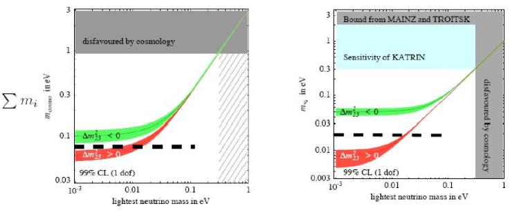
Figure 7: The effective mass measured in double $\beta$ decay, in cosmology and in Tritium $\beta$ decay versus the mass of the lightest neutrino. Below the dashed lines, only the normal hierarchy is allowed.

Neutrino-less double beta decay experiments, see [23] for a review, do not measure the absolute mass of the neutrino directly but a combination of neutrino masses and mixings,

$$m_{\beta\beta}=\mid\sum m_{i}U_{ei}^{2}\mid=\mid m_{a}c_{13}^{2}c_{12}^{2}+m_{2}c_{13}^{2}s_{12}^{2}e^{2i\alpha}+m_{3}s_{13}^{2}e^{2i\beta}\mid,$$ (66)

where it is understood that neutrinos are taken to be Majorana particles. The new generation of experiments seeks to reach below 10 meV for $m_{\beta\beta}$ in double beta decay.

Cosmological probes measure the sum of the neutrino masses,

$$m_{\mbox{cosmo}}=\sum_{i}m_{i}.$$ (67)

If $\sum m_{i}\approx 50$ eV, the energy balance of the universe saturates the bound coming from its critical density. The current limit, [24], is a few % of this number, $\sim 1$ eV. These bounds are model dependent but they do all give numbers of the same order of magnitude. However, given the systematic uncertainties characteristic of cosmology, a solid limit of less that 100 meV seems way too aggressive.

Fig. 7 shows the allowed parameter space for the neutrino masses (as a function of the absolute scale) for both the normal and inverted hierarchy.

0.6.2 Majorana vs Dirac

A fermion mass is nothing but a coupling between a left handed state and a right handed one. Thus, if we examine a massive fermion at rest, then one can regards this state as a linear combination of two massless particles, one right handed and one left handed particle. If the particle we are examining is electrically charged, like an electron, both particles, the left handed as well as the right handed must have the same charge (we want the mass term to be electrically neutral). This is a Dirac mass term. However, for a neutral particle, like a sterile neutrino, a new possibility opens up, the left handed particle can be coupled to the right handed anti-particle, (a term which would have a net charge, if the fields are not absolutely and totally neutral) this is a Majorana mass term.

Thus a neutral particle does have two ways of getting a mass term, a la Dirac or a la Majorana, and in principle can have them both, as shown :

In the case of a neutrino, the left chiral field couples to $SU(2)\times U(1)$ implying that a Majorana mass term is forbidden by gauge symmetry. However, the right chiral field carries no quantum numbers, is totally and absolutely neutral. Then, the Majorana mass term is unprotected by any symmetry and it is expected to be very large, of the order of the largest scale in the theory. On the other hand, Dirac mass terms are expected to be of the order of the electroweak scale times a Yukawa coupling, giving a mass of the order of magnitude of the charged lepton or quark masses. Putting all the pieces together, the mass matrix for the neutrinos results as in Fig. 8.

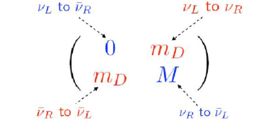
Figure 8: The neutrino mass matrix with the various right to left couplings, $M_{D}$ is the Dirac mass terms while 0 and $M$ are Majorana masses for the charged and uncharged (under $SU(2)\times U(1)$) chiral components.

To get the mass eigenstates we need to diagonalise the neutrino mass matrix. By doing so, one is left with two Majorana neutrinos, one super-heavy Majorana neutrino with mass $\simeq M$ and one light Majorana neutrino with mass $m_{D}^{2}/M$, i.e. one mass goes up while the other sinks, this is what we call the seesaw mechanism, [25, 26, 27]. The light neutrino(s) is(are) the one(s) observed in current experiments (its mass differences) while the heavy neutrino(s) are not accessible to current experiments and could be responsible for explaining the baryon asymmetry of the universe through the generation of a lepton asymmetry at very high energy scales since its decays can in principle be CP violating (they depend on the two Majorana phases on the PNMS matrix which are invisible for oscillations).

If neutrinos are Majorana particles lepton number is no longer a good quantum number and a plethora of new processes forbidden by lepton number conservation can take place, it is not only neutrino-less double beta decay. For example, a muon neutrino can produce a positively charged muon. However, this process and any processes of this kind, would be suppressed by $(m_{\nu}/E)^{2}$ which is tiny, $10^{-20}$, and therefore, although they are technically allowed, are experimentally unobservable.

0.7 Conclusions

The experimental observations of neutrino oscillations, meaning that neutrinos have mass and mix, answered questions that had endured since the establishment of the Standard Model. As those veils have disappeared, new questions open up and challenge our understanding:

• what is the nature of the neutrino? are they Majorana or Dirac? are neutrinos totally neutral?

• is the spectrum normal or inverted?

• is CP violated (is $\sin\delta\neq 0$)?

• which is the absolute mass scale of the neutrinos?

• are there new interactions?

• can neutrinos violate CPT [28]?

• are these intriguing signals in short baseline reactor neutrino experiments (the missing fluxes) a real effect? Do they imply the existence of sterile neutrinos?

We would like to answer these questions. For doing it, we are doing right now, and we plan to do new experiments. These experiments will, for sure bring some answers and clearly open new, pressing questions. Only one thing is clear. Our journey into the neutrino world is just beginning.

References

- [1] Z. Maki, M. Nakagawa and S. Sakata, Prog. Theor. Phys. 28, 870 (1962).
- [2] H. J. Lipkin, Phys. Lett. B 579, 355 (2004) [arXiv:hep-ph/0304187].
- [3] L. Stodolsky, Phys. Rev. D 58, 036006 (1998) [arXiv:hep-ph/9802387].
- [4] An analysis of CPT violation in the neutrino sector can be found in: G. Barenboim and J. D. Lykken, Phys. Lett. B 554 (2003) 73 [arXiv:hep-ph/0210411] ; G. Barenboim, J. F. Beacom, L. Borissov and B. Kayser, Phys. Lett. B 537 (2002) 227 [arXiv:hep-ph/0203261].
- [5] See for example, Neutrino mass, by B.Kayser, in D. E. Groom et al. [Particle Data Group], Eur. Phys. J. C 15, 1 (2000).
- [6] L. Wolfenstein, Phys. Rev. D 17, 2369 (1978).
- [7] S. P. Mikheev and A. Y. Smirnov, “Resonance enhancement of oscillations in matter and solar neutrino Sov. J. Nucl. Phys. 42, 913 (1985) [Yad. Fiz. 42, 1441 (1985)].
- [8] S. P. Mikheev and A. Y. Smirnov, “Neutrino oscillations in a variable-density medium and bursts due Sov. Phys. JETP 64, 4 (1986) [Zh. Eksp. Teor. Fiz. 91, 7 (1986)] [arXiv:0706.0454 [hep-ph]].
- [9] S. P. Mikheev and A. Y. Smirnov, “Resonant amplification of neutrino oscillations in matter and solar Nuovo Cim. C 9, 17 (1986).
- [10] N. Tolich [SNO Collaboration], J. Phys. Conf. Ser. 375 (2012) 042049.
- [11] F. P. An et al. [DAYA-BAY Collaboration], Phys. Rev. Lett. 108 (2012) 171803 [arXiv:1203.1669 [hep-ex]].
- [12] Y. Ashie et al. [Super-Kamiokande Collaboration], “A measurement of atmospheric neutrino oscillation parameters by Phys. Rev. D 71, 112005 (2005) [arXiv:hep-ex/0501064]; Y. Takeuchi [Super-Kamiokande Collaboration], arXiv:1112.3425 [hep-ex].
- [13] E. Aliu et al. [K2K Collaboration], “Evidence for muon neutrino oscillation in an accelerator-based Phys. Rev. Lett. 94, 081802 (2005) [arXiv:hep-ex/0411038].
- [14] M. H. Ahn et al. [K2K Collaboration], Phys. Rev. Lett. 90, 041801 (2003) [arXiv:hep-ex/0212007]; M. H. Ahn et al. [K2K Collaboration], Phys. Rev. D 74 (2006) 072003 [hep-ex/0606032].
- [15] D. Naples [MINOS Collaboration], J. Phys. Conf. Ser. 375 (2012) 042073.
- [16] K. Eguchi et al. [KamLAND Collaboration], “First results from KamLAND: Evidence for reactor anti-neutrino Phys. Rev. Lett. 90, 021802 (2003) [arXiv:hep-ex/0212021].
- [17] T. Araki et al. [KamLAND Collaboration], “Measurement of neutrino oscillation with KamLAND: Evidence of spectral Phys. Rev. Lett. 94, 081801 (2005) [arXiv:hep-ex/0406035].
- [18] B. Aharmim et al. [SNO Collaboration], “Electron energy spectra, fluxes, and day-night asymmetries of B-8 solar Phys. Rev. C 72, 055502 (2005) [arXiv:nucl-ex/0502021].
- [19] S. Fukuda et al. [Super-Kamiokande Collaboration], “Determination of solar neutrino oscillation parameters using 1496 days of Phys. Lett. B 539, 179 (2002) [arXiv:hep-ex/0205075].
- [20] S. J. Parke and T. P. Walker, Phys. Rev. Lett. 57, 2322 (1986) [Erratum-ibid. 57, 3124 (1986)].
- [21] M. Apollonio et al. [CHOOZ Collaboration], Phys. Lett. B 466, 415 (1999) [arXiv:hep-ex/9907037].
- [22] A. Osipowicz et al. [KATRIN Collaboration], [arXiv:hep-ex/0109033.]
- [23] S. R. Elliott and P. Vogel, Ann. Rev. Nucl. Part. Sci. 52, 115 (2002) [arXiv:hep-ph/0202264].
- [24] D. N. Spergel et al. [WMAP Collaboration], “Wilkinson Microwave Anisotropy Probe (WMAP) three year results: Astrophys. J. Suppl. 170, 377 (2007) [arXiv:astro-ph/0603449].
- [25] M. Gell-Mann, P. Ramond and R. Slansky, in Supergravity, edited by P.van Nieuwenhuizen and D. Freedman, (North-Holland,1979), p.315.
- [26] R. N. Mohapatra and G. Senjanovic, Phys. Rev. Lett. 44, 912 (1980).
- [27] M. Fukugita and T. Yanagida, Phys. Lett. B 174, 45 (1986).
- [28] G. Barenboim, L. Borissov, J. D. Lykken and A. Y. Smirnov, JHEP 0210 (2002) 001 [hep-ph/0108199]. G. Barenboim and J. D. Lykken, Phys. Rev. D 80 (2009) 113008 [arXiv:0908.2993 [hep-ph]].