Efficient Interference Management Policies for Femtocell Networks

Abstract

Managing interference in a network of macrocells underlaid with femtocells presents an important, yet challenging problem. A majority of spatial frequency/time reuse based approaches partition the users by coloring the interference graph, which is shown to be suboptimal. Some spatial time reuse based approaches schedule the maximal independent sets (MISs) of users in a cyclic, (weighted) round-robin fashion, which is inefficient for delay-sensitive applications. Our proposed policies schedule the MISs in a non-cyclic fashion, which aim to optimize any given network performance criterion for delay-sensitive applications while fulfilling minimum throughput requirements of the users. Importantly, we do not take the interference graph as given as in existing works; we propose an optimal construction of interference graph. We prove that under certain conditions, the proposed policy achieves the optimal network performance. For large networks, we propose a low-complexity algorithm for computing the proposed policy, and prove that under certain conditions, the policy has a competitive ratio (with respect to the optimal network performance) that is independent of the network size. The proposed policy can be implemented in a decentralized manner by the users. Compared to the existing policies, our proposed policies can achieve improvement of up to 130 % in large-scale deployments.

I Introduction

As more and more devices are connecting to cellular networks, the demand for wireless spectrum is exploding. Dealing with this increased demand is especially difficult because most of the traffic comes from bandwidth-intensive and delay-sensitive applications such as multimedia streaming, video surveillance, video conferencing, gaming etc. These demands make it increasingly challenging for the cellular operators to provide sufficient quality of service (QoS). Dense deployment of distributed low-cost femtocells (or small cells in general, such as microcells and picocells) has been viewed as one of the most promising solutions for enhancing access to the radio spectrum[1][2]. Femtocells are attractive because they can both extend the service coverage and boost the network capacity by shortening the access distance (cell splitting gain) and offloading traffic from the cellular network (offloading gain). However, in a closed access network when only registered mobile users can connect to the femtocell base station, dense deployment of femtocells operating in the same frequency band leads to strong co-tier interference. In addition, the macrocell users usually operate in the same frequency, the problem of interference (to both femtocells and macrocells) is further exacerbated due to cross-tier interference across macrocells and femtocells. In this work, we study a closed access network. Hence, it is crucial to design interference management policies to deal with both co-tier and cross-tier interference.

Interference management policies specify the transmission schedule and transmit power levels of femtocell user equipments FUEs (femtocell base stations FBSs) and macrocell user equipments MUEs (macrocell base stations MBSs) in uplink (downlink) transmissions. An efficient interference management policy should fulfill the following important requirements (we will discuss in Section II, state-of-the-art policies do not fulfill one or more of the following requiremenst):

• Interference management based on network topology: Policies must take into account that uplink transmissions from neighboring UEs create strong mutual interference, but must also recognize and take advantage of the fact that non-neighboring UEs do not. Hence, the network topology (i.e. locations of femtocells/macrocells) must play a crucial role.

• Limited signaling for interference coordination: In dense, large-scale femtocell deployments, the UEs cannot coordinate their transmissions by sending a large amount of control signals across the network. Hence, effective policies should not rely on heavy signaling and/or message exchanges across the UEs in the network.

• Scalability in large networks: Femtocell networks are often deployed on a large scale (e.g. in a city). Effective policies should scale in large networks, i.e. achieve efficient network performance while maintaining low computational complexity.

• Support for delay-sensitive applications: Effective policies must support delay-sensitive applications, which constitute the majority of wireless traffic.

• Versatility in optimizing various network performance criteria: The appropriate network performance criterion (e.g. weighted sum throughput, max-min fairness, etc.) may be different for different networks. Effective policies should be able to optimize a variety of network performance criteria while ensuring performance guarantees for each MUE and each FUE.

In this work, we propose a novel, systematic, and practical methodology for designing and implementing interference management policies that fulfill all of the above requirements. Our proposed policies aim to optimize a given network performance criterion, such as weighted sum throughput and max-min fairness, subject to each UE’s minimum throughput requirements. Our proposed policies can efficiently manage a wide range of interference. We manage strong interference between neighboring UEs by using time-division multiple access (TDMA) among them. We take advantage of weak interference between non-neighboring UEs by finding maximal sets of UEs that do not interfere with each other and allowing all the UEs in those sets to transmit at the same time. Specifically, we find the maximal independent sets (MISs) of the interference graph, and schedule different MISs to transmit in different time slots. The scheduling of MISs in our proposed policy is particularly designed for delay-sensitive applications: the schedule of MISs across time is not cyclic (i.e. the policies do not allocate transmission times to MISs in a fixed (weighted) round-robin manner), but rather follows a carefully designed nonstationary schedule, in which the MIS to transmit is determined adaptively online. For delay-sensitive applications, cyclic policies are inefficient because transmission opportunities (TXOPs) earlier in the cycle are more valuable than TXOPs later in the cycle (earlier TXOPs enhances the chances of transmission before delay deadlines). The cyclic polices are unfair to UEs allocated to later TXOPs.

Another distinctive feature of our work is that we do not take the interference graph as given as in most existing works; instead, in our work we show how to choose the interference graph that maximizes the network performance. Specifically, in our construction of interference graphs, we determine how to choose the threshold on the distance between two cells, based on which we determine if there is an edge between them, in order to maximize the network performance. Moreover, we prove that under certain conditions, the proposed policy, computed based on the optimal threshold, can achieve the optimal network performance (weighted sum throughput) within a desired small gap. Note that for large networks, in general it is computationally intractable to find all the MISs of the interference graph [3]. We propose efficient polynomial-time algorithms to find a subset of MISs, and prove that under certain conditions, the proposed policy, computed based on the constructed subset of MISs, can achieve a constant competitive ratio (with respect to optimal weighted sum throughput) that is independent of the network size.

Finally, we summarize the main contributions of our work:

1. We propose interference management policies that schedule the MISs of the interference graph. The schedule is constructed in order to maximize the network performance criterion subject to minimum throughput requirements of the UEs. Moreover, the schedule adapts to the delay sensitivity requirements of the UEs by scheduling transmissions in a non-stationary manner.

2. We construct the interference graph by comparing the distances between the BSs with a threshold (i.e. there is an edge between two cells if the distance between their BSs is smaller than the threshold). We develop a procedure to choose the optimal threshold such that the proposed scheduling of MISs leads to a high network performance. Importantly, we prove that under certain conditions, the proposed scheduling of MISs based on the optimal threshold achieves within a desired small gap of the optimal network performance (weighted sum throughput).

3. It is intractable to find all the MISs in large networks, we propose an approximate algorithm that computes a subset of MISs within polynomial time. We prove that under certain conditions, the proposed policy based on this subset of MISs has a constant competitive ratio (with respect to the optimal weighted sum throughput) that is independent of the network size.

The rest of the paper is organized as follows. In Section II we discuss the related works and their limitations followed by the system model and problem formulation in Section III and IV respectively. The design framework and its low-complexity variant for large networks are discussed in Section V and Section VI respectively. In Section VII we use simulations to compare the proposed policy with state-of-the-art followed by conclusion in Section VIII.

II Related Works

In this section we compare our proposed policy with state-of-the-art policies. Existing interference management policies can be categorized in two classes: 1) policies based on power control, and 2) policies based on spatial time/frequency reuse.

II-A Interference Management Policies Based on Power Control

The first and most widely-used interference management policies[4, 5, 6, 7, 8, 9, 10] are based on power control. In these policies, all the UEs in the network transmit at a constant power at all time (provided that the system parameters remain the same) in the entire frequency band . When the cross channel gains among BSs and UEs are high, simultaneous transmissions at the same time and in the same frequency band will cause significant interference among cells. Such strong interference is common in macrocells underlaid with femtocells. For example, in [11] it is shown that that interference from MUEs near the FBS severely affects the uplink transmissions of FUEs. Also, in offices and apartments, where FBSs are installed close to each other, inter-cell interference is particularly strong. In contrast, our proposed solutions mitigate the strong interference by letting only a subset of non-interfering UEs to transmit at the same time.

II-B Interference Management Policies Based on Spatial Time/Frequency Reuse

Some existing works mitigate strong interference by letting different subsets of UEs to transmit in different time slots (spatial time reuse) [12, 13, 14, 15, 16, 17, 18, 19, 20] or in different frequency channels (spatial frequency reuse) [21, 22, 23, 24, 25, 26, 27]. Specifically, they partition UEs into disjoint subsets such that the UEs in the same subset do not interfere with each other. Given the same partition of the UEs, the policies based on spatial time reuse and those based on spatial frequency reuse are equivalent. Hence, we focus on policies based on spatial time reuse hereafter.

Some policies based on spatial time reuse, partition the UEs based on the coloring of the interference graph h [12, 13, 14, 15, 16], which is not efficient. In general, a set of UEs with the same color (i.e. the UEs who can transmit simultaneously) may not be maximal (See Fig. 1 a), in the sense that there may be UEs who do not interfere but have different colors (we will also show this in the motivating example in Subsection IV-B). In this case, it is more efficient to also let those non-interfering UEs to transmit simultaneously, although they have different colors. Hence, the partitioning based on coloring the interference graph is not efficient, because the average number of active UEs (i.e. the average cardinality of the subsets of UEs with the same color) is low.

Some policies based on spatial time reuse[17, 18, 20, 19] partition the UEs based on the MISs of the interference graph, which is more efficient, because we cannot add any more UEs to an MIS without creating strong interference. However, they are still inefficient compared to our proposed policies for delay-sensitive applications. Specifically, they schedule different MISs in a cyclic and (weighted) round-robin manner, in which each UE transmits at a fixed position in each cycle. For delay-sensitive applications, earlier positions in the cycle are more desirable because they enhance the chances of transmitting prior to delay deadlines. Hence, a cyclic schedule is not fair to the UEs allocated to later positions. In contrast, our proposed policies schedule the MISs in an efficient, nonstationary manner for delay-sensitive applications.

Another notable difference from the existing works based on spatial time/frequency reuse is that they usually take the interference graph as given. On the contrary, our work discusses how to construct the interference graph optimally such that the network performance is maximized.

II-C Other Interference Management Policies

Besides the above two categories, there are several other related works. For instance in [28][29], the authors propose reinforcement learning and evolutionary learning techniques for the femtocells to learn efficient interference management policies. In [28], the femtocells learn the fixed transmit power levels, while in [29], the femtocells learn to randomize over different transmit power levels. However, the interference management policies in [28] and [29] cannot provide minimum throughput guarantees for the UEs. In constrast, we provide rigorous minimum throughput guarantees for the UEs. In both [28][29] the femtocell UEs need to limit their transmission powers in every time slot such that the SINR of the macrocell UE is sufficiently high. If there is strong interference between some femtocells and the macrocell, the femtocell UEs will always transmit at lower power levels, leading to a low sum throughput for them.

Another method to mitigate interference is to deploy coordinated beam scheduling [30][31]. In [30] and [31], the authors schedule a subset of beams to maximize the total reward associated with the scheduled subset, where the reward per beam reflects the channel quality and traffic. The first difference from our work is that the proposed approach schedules a fixed subset of beams and leaves the other UEs inactive. Hence, some UEs have no throughput, which means the minimum throughput as well as the delay-sensitivity of the UEs is not satisfied. Second, we rigorously prove that our proposed policy achieves good performance with low (polynomial-time) complexity , while [30][31] do not. Third, the schemes in [30][31] are proposed for a specific network performance criterion and may not be flexible enough for other network performance criteria (such as the sum throughput). Finally, [30][31] do not consider delay sensitivity of the UEs.

III System Model

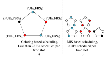
Fig. 1 a)

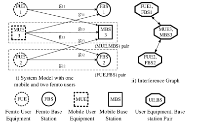
Fig. 1 b)

Figure 1: a) Coloring based scheduling in i) schedules less than two UEs per time slot on an average, while MIS based scheduling in ii) is more efficient and schedules two UEs per time slot. , b) System model illustration.

III-A Heterogeneous Network of Macrocells and Femtocells

We consider a heterogeneous network of $N$ femtocells (indexed by $\{1,2,\ldots,N\}$) and $M$ macrocells (indexed by $\{N+1,...,N+M\}$) operating in the same frequency band, a common deployment scenario considered in practice [4]. We assume that each FBS/MBS serves only one FUE/MUE . Our model can be easily generalized to the setting where each BS serves multiple UEs, at the expense of complicated notations to denote the association among UEs and BSs. For notational clarity, we focus on the case where each BS serves one UE, and will demonstrate the applicability of our work to the setting where one BS serves multiple UEs in Section VII.

Since there is only one FUE or MUE in a femtocell or a macrocell, the index of each UE and that of each BS are the same as the index of the cell they belong to. We focus on the uplink transmissions. The proposed framework can be applied directly to the downlink scenarios in which each BS serves one UE at a time. See Fig. 1b) for an illustration of a 3-cell network with $N=2$ femtocells and $M=1$ macrocell. Each UE $i$ chooses its transmit power $p_{i}$ from a compact set $\mathcal{P}_{i}\subseteq\mathbb{R}_{+}$. We assume that $0\in\mathcal{P}_{i},\;\forall i\;\in\{1,...N+M\}$, namely a UE can choose not to transmit. The joint power profile of all the UEs is denoted by $\textbf{p}=(p_{1},....p_{N+M})\in\mathcal{P},$ where $\mathcal{P}=\prod_{i=1}^{N+M}\mathcal{P}_{i}$. The power profile of all the UEs other than $i$ is denoted by $\textbf{p}_{-i}$. When a UE $i$ chooses a transmit power $p_{i}$, the signal to interference and noise ratio (SINR) experienced at BS $i$ is $\gamma_{i}(\textbf{p})=\frac{g_{ii}p_{i}}{\sum\limits_{j\not=i}g_{ji}p_{j}+\sigma_{i}^{2}}$, here $g_{ji}$ is the channel gain from UE $j$ to BS $i$, and $\sigma_{i}^{2}$ is the noise power at BS $i$. Since the BSs cannot cooperate to decode their messages, each BS $i$ treats the interference as white noise, and gets the following throughput [4] $r_{i}(\textbf{p})=\log_{2}(1+\gamma_{i}(\textbf{p}))$.

III-B Interference Management Policies

The system is time slotted at $t$ = 0,1,2…, and the UEs are assumed to be synchronized as in [32]. At the beginning of time slot $t$, each UE $i$ decides its transmit power $p_{i}^{t}$ and obtains a throughput of $r_{i}(\textbf{p}^{t})$. Each UE $i$’s strategy, denoted by $\pi_{i}:\mathbb{Z}_{+}=\{0,1,..\}\rightarrow\mathcal{P}_{i}$, is a mapping from time $t$ to a transmission power level $p_{i}\in\mathcal{P}_{i}$. The interference management policy is then the collection of all the UEs’ strategies, denoted by $\boldsymbol{\pi}=(\pi_{1},...,\pi_{N+M})$. Each UE is ${\it{delay\;sensitive}}$ and hence discounts the future throughputs as in [33]. The average discounted throughput for UE $i$ is given as $R_{i}(\boldsymbol{\pi})=(1-\delta)\sum\limits_{t=0}^{\infty}\delta^{t}r_{i}(\textbf{p}^{t}),$where $\textbf{p}^{t}=(\pi_{1}(t),...,\pi_{N+M}(t))$ is the power profile at time $t$, and $\delta\in[0,1)$ is the discount factor assumed to be the same for all the UEs as in [32, 33]. We also assume the channel gain to be fixed over the considered time horizon as in [18, 19, 22][32, 33]. We will illustrate in Section VI-D and Section VII-C that the proposed framework can be adapted to the scenarios in which the channel conditions are time-varying.

An interference management policy $\bm{\pi}^{const}$ is a policy based on power control [4], if $\bm{\pi}(t)=\textbf{p}$ for all $t$. Write the joint throughput profile of all the UEs as $\textbf{r}(\textbf{p})=(r_{1}(\textbf{p}),...,r_{N+M}(\textbf{p}))$. Then the set of all joint throughput profiles achievable by policies based on power control can be written as $\mathcal{R}^{const}=\{\textbf{r}(\textbf{p}),\;\textbf{p}\in\mathcal{P}\}$. As we have discussed before, our proposed policy is based on MISs of the interference graph. The interference graph $G$ has $M+N$ vertices, which are the $M+N$ cells. There is an edge between two cells if their cross interference is high. We will describe in detail how to construct the interference graph in Section V. Given an interference graph, we write $\textbf{I}^{G}=\{I_{1}^{G},...,I_{s(G)}^{G}\}$ as the set of all the MISs of the interference graph. Let $\textbf{p}^{I_{j}^{G}}$ be a power profile in which the UEs in the MIS $I_{j}^{G}$ transmit at their maximum power levels, namely $p_{k}=p_{k}^{max}\triangleq\max\mathcal{P}_{k}\;\text{if}\;k\in I_{j}^{G}$ and $p_{k}=0$ otherwise. Let $\mathcal{P}^{MIS(G)}=\{\textbf{p}^{I_{1}^{G}},...,\textbf{p}^{I_{s(G)}^{G}}\}$ be the set of all such power profiles. Then $\bm{\pi}$ is a policy based on MIS if $\bm{\pi}(t)\in\mathcal{P}^{MIS(G)}$ for all $t$. We denote the set of policies based on MISs by $\Pi^{MIS(G)}=\{\boldsymbol{\pi}:\mathbb{Z}_{+}\rightarrow\mathcal{P}^{MIS(G)}\}$. The set of joint $instantaneous$ throughput profiles achievable by policies based on MIS is then $\mathcal{R}^{MIS(G)}=\{\textbf{r}(\textbf{p}):\;\textbf{p}\in\mathcal{P}^{MIS(G)}\}$. We will prove in Theorem 1 that the set of joint discounted throughput profiles achievable by policies based on MIS is $\mathcal{V}^{MIS(G)}=\text{conv}\{\mathcal{R}^{MIS(G)}\}$, where $\text{conv}\{X\}$ representing the convex hull of set $X$.

IV Problem Formulation

In this section, we formalize the interference management policy design problem, and subsequently give a motivating example to highlight the advantages of the proposed policy over existing policies in solving this problem.

IV-A Policy Design Problem

The designer of the network (e.g. the network operator) aims to design an optimal interference management policy $\boldsymbol{\pi}$ that fulfills each UE $i$’s minimum throughput requirement $R_{i}^{min}$ and optimizes a chosen network performance criterion $W(R_{1}(\boldsymbol{\pi}),....,R_{N+M}(\boldsymbol{\pi}))$. The network performance criterion $W$ is an increasing function in each $R_{i}$. For instance, $W$ can be the weighted sum of all the UEs’ throughput, i.e.$\sum_{i=1}^{N}w_{i}^{FUE}R_{i}(\boldsymbol{\pi})+\sum_{j=1}^{M}w_{j}^{MUE}R_{N+j}(\boldsymbol{\pi})$ with $\sum_{i=1}^{N}w_{i}^{FUE}+\sum_{j=1}^{M}w_{j}^{MUE}=1$ and $w_{i}^{MUE},w_{j}^{FUE}\geq 0$ . We emphasize that the higher-priority of MUEs can be reflected by setting higher weights for the MUEs (i.e. $w_{i}^{MUE}\geq w_{j}^{FUE}\,\forall i=\{1,\ldots,N\},\,\forall j=\{1,\ldots,M\}$), and by setting higher minimum throughput requirements for MUEs. The performance criterion $W$ can also be max-min fairness (i.e., the worst UE’s throughput $\min_{i}R_{i}(\boldsymbol{\pi})$) or the proportional fairness. The policy design problem is given as follows.

$$\mathbf{Design\,Problem} \max_{\boldsymbol{\pi}} W(R_{1}(\boldsymbol{\pi}),....,R_{N+M}(\boldsymbol{\pi}))$$

$$s.t. R_{i}(\boldsymbol{\pi})\geq R_{i}^{min},\forall i\in\{1,...,N+M\}$$

The key steps and the challenges in solving the design problem are as follows: 1) How to determine the set of achievable throughput profiles? Note that the set depends on the discount factor $\delta$. It is an open problem to determine the set of achievable throughput profiles, even for the special case of $\delta=0$ (i.e. the set of throughput profiles achievable by policies based on power control). 2) How to construct the optimal policy that achieves the optimal target throughput profile? The optimal policy again depends on $\delta$. It is much more challenging to determine the policy for delay-sensitive applications (i.e. $\delta<1$) than for delay-insensitive applications (i.e. $\delta\rightarrow 1$), because the optimal policy is not cyclic. 3) How to construct a distributed policy with minimum communication overhead?

IV-B Motivating Example

We consider a network of 5 femtocells. On the left plot of Fig. 1 a), we have portrayed the interference graph of this network. Each vertex denotes a pair of FBS and its FUE. Each edge denotes strong local interference between the connected vertices (i.e. the distance between the FBSs is below some threshold). The interference graph is a pentagon, where each UE interferes only with two neighbors. We show the partitioning of the UEs by coloring the interference graph. There are three colors, and there is one color (i.e. black) to which only one UE belongs. On the right plot of Fig. 1 a), we show the 5 MIS’s, each of which consists of two UEs. Note that the MIS are not disjoint. For illustrative purposes, suppose that the 5 femtocells and their UEs are symmetric, in the sense that all the UEs have maximum transmit power of 30mW, direct channel gain of 1, cross channel gain of 0.25 between the neighbors, noise power at the receiver of 2mW, minimum throughput requirement of 1.2 bits/s/Hz, and discount factor of 0.8 representing delay sensitivity. For simplicity, we set the cross channel gain between non-neighbors to be 0.

We compare our proposed policy against the following policies discussed in Section II:

• Policies based on power control [4][34], in which each UE chooses a constant (time-invariant) power level all the time.

• Coloring-based TDMA policies [12][16], in which the UEs are partitioned into mutually exclusive subsets by coloring the interference graph; in each time slot, all the UEs of one color are chosen to transmit. In this example, 3 colors are required and there will always exist a color to which only one UE belongs. Hence, the average number of active UEs in each time slot is less than 2. Note that the optimal performance of coloring based frequency reuse policies is the same as the optimal performance that can be attained by any coloring based TDMA of any arbitrary cycle length. This is due to the fact that FDM and TDM are equivalent provided the frequency/time can be divided arbitrarily.

• Cyclic MIS-based TDMA policies [18][19], in which different MISs of UEs are scheduled in a cyclic manner. In this example, there are 5 MISs, each of which consists of 2 UEs. Hence, the average number of active UEs in each time slot is 2. This is the major reason why MIS-based TDMA policies are more efficient than coloring-based TDMA policies. To completely specify the policy we must also specify a cycle length and order of transmissions; note that the efficiency of the policy will depend on the cycle length due to delay sensitivity.

We illustrate the performance of the above policies vs the proposed policy in Table 1. Remarkably, the proposed policy is not only much more efficient than existing policies, it is much easier to compute. To compare with constant policies, note simply that finding the optimal constant policy is intractable [34] in general, because the optimization problem is non-convex due to the mutual interference. To compare with different classes of TDMA policies, note that for (coloring-based and MIS-based) cyclic TDMA policies, the complexity of finding the optimal cyclic policy of a given length grows exponentially with the cycle length (and exponentially with the number of MISs when the cycle length is large enough for reasonable performance). To get a hint of why this is so, note that in a cyclic policy, the UE’s performance is determined not only by the number of TXOPs in a cycle but also by the positions of the TXOPs since UEs are discounting their future utilities (due to delay sensitivity). Thus, it is not only the length of the cycle that is important but also the ordering of transmissions within each cycle. For instance, for the 5-UE case above, achieving performance within 10% of the optimal nonstationary policy requires that the cycle length L be at least 7, and so requires searching among the thousands (16800) of different nontrivial schedules (the schedules in which each UE transmits at least once in each cycle) of cycle length 7. Even this small problem is computationally intensive. For a moderate number of 10 femtocells, assuming a completely connected interference graph which has 10 MISs, and a cycle length of 20, we need to search more than ten billion (i.e. $10^{10}$) non-trivial schedules – a completely intractable problem.

Table I: Comparisons against spatial reuse TDMA based policies

Policies	Max-min throughput (bits/s/Hz)	Performance Gain %
Optimal constant power	1.32	21.2%
Optimal Coloring TDMA (arbitrary L)	1.33 (Upper Bound)	20.3 %
Optimal MIS TDMA (L=5)	1.36	17.6 %
Optimal MIS TDMA (L=7)	1.49	7.8  %
Optimal Proposed	1.60	–

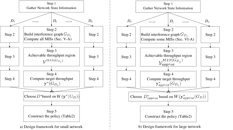
Figure 2: Steps in the design framework.

V Design Framework

In this section, we develop the general design framework for solving the design problem (1). We will provide sufficient conditions under which our proposed framework is optimal, and demonstrate a wide variety of networks that fulfill the sufficient conditions.

V-A Description of the Proposed Design Framework

The proposed methodology for solving the design problem consists of 5 steps which are illustrated in Fig. 2 . We describe them in detail as follows.

V-A1 Step 1. The Designer Gathers Network Information

The designer is informed by each BS $i$ of the minimum throughput requirement $R_{i}^{min}$ of its UE, the channel gain from each UE $j$ to its receiver $g_{ji}$, its UE’s maximum transmit power level $p_{i}^{max}$, the noise power level at its receiver $\sigma_{i}^{2}$, and its location as in [22][23]. Such information is sent to the designer via the backhaul link. In some circumstances, the information about the location of FBSs is available to the femtocell gateways [23], who can send this information to the designer.

V-A2 Step 2. The Designer Constructs the Interference Graph and Computes the MISs

The designer constructs the interference graph using the information of cell locations obtained in Step 1. Specifically, it uses a distance based threshold rule as in [13][35] to construct the graph: there is an edge between two cells if the distance between BSs in these two cells is smaller than a threshold $D$ . Given the threshold $D$, we denote the resulting graph by $G_{D}$, and the set of its MISs by $\textbf{I}^{G_{D}}$, which can be calculated as in [3]. We assume that the distance threshold $D$ is fixed for now, and will discuss how to select the threshold in the next subsection.

V-A3 Step 3. The Designer Characterizes Achievable Throughput

Based on the MISs  computed in Step 2, the designer identifies the set $\mathcal{V}^{MIS(G_{D})}(\delta)$ of throughput vectors achievable by MIS-based policies. Note that $\mathcal{V}^{MIS(G_{D})}(\delta)$ depends on the discount factor. Recall that $\mathcal{R}^{MIS(G_{D})}=\{\textbf{r}(\textbf{p}):\;\textbf{p}\in\mathcal{P}^{MIS(G_{D})}\}$ is the set of instantaneous throughput profiles achievable by MIS-based policies in $\Pi^{MIS(G_{D})}$. The theorem below proves that $\mathcal{V}^{MIS(G_{D})}(\delta)$ is a convex hull of $\mathcal{R}^{MIS(G_{D})}$, i.e. $\mathcal{V}^{MIS(G_{D})}$ when the discount factor $\delta\geq 1-\frac{1}{s(G_{D})}$, where $s(G_{D})$ is the number of MISs in the interference graph $G_{D}$.

Theorem 1: Given the interference graph $G_{D}$, for any $\delta\geq\bar{\delta}=1-\frac{1}{s(G_{D})}$, the set of throughput profiles achieved by MIS-based policies is $\mathcal{V}^{MIS(G_{D})}(\delta)=\mathcal{V}^{MIS(G_{D})}$.

See the detailed proof in the Appendix at the end.

Proof Sketch: The main step involved in proving the above is to derive the conditions on the discount factor such that each throughput vector in $\mathcal{V}^{MIS(G_{D})}$ can be decomposed into a current throughput vector which belongs to $\mathcal{R}^{MIS(G_{D})}$ and a continuation throughput which belongs to $\mathcal{V}^{MIS(G_{D})}$. To derive the conditions, we show that for any vector in $\mathcal{V}^{MIS(G_{D})}$ there exists at least one throughput vector in $\mathcal{R}^{MIS(G_{D})}$ to decompose the vector. Since the continuation throughput also belongs to $\mathcal{V}^{MIS(G_{D})}$, it can be decomposed as well in a similar fashion. Hence, all the vectors in $\mathcal{V}^{MIS(G_{D})}$ are achievable.

Theorem 1 is important, because it analytically characterizes the set of throughput profiles achievable by MIS-based policies, and gives us the requirements that need to be fulfilled by the discount factor.

V-A4 Step 4. The Designer Determines the Optimal Target Weights

Among all the achievable throughput profiles identified in Step 3, the designer selects the target throughput profile in order to optimize the network performance. Note that each UE $i$’s average throughput $R_{i}$ can be expressed as a convex combination of the instantaneous throughput vectors achieved by MIS-based policies (i.e. the throughput vectors in $\mathcal{R}^{MIS(G_{D})}$). Thus, determining the optimal target vector and its corresponding coefficient can be formulated as the following optimization problem :

$$\max_{\boldsymbol{y},\boldsymbol{\alpha}}\,\, W(y_{1}(G_{D}),...,y_{N+M}(G_{D}))$$

$$s.t.\,\, y_{i}(G_{D})\geq R_{i}^{min},\;\forall i\in\{1,...,N+M\}$$

$$y_{i}(G_{D})=\sum_{j=1}^{s(G_{D})}\alpha_{j}r_{i}(\textbf{p}^{I_{j}^{G_{D}}}),\forall i\in\{1,....,N+M\}$$ (2)

$$\sum_{j=1}^{s(G_{D})}\alpha_{j}=1,\,\alpha_{j}\geq 0,\;\forall j\in\{1,..,s(G_{D})\}$$

The above optimization problem is a convex optimization problem and is easy to solve if $W$ is concave (e.g. weighted sum throughput or max-min fairness). The resulting optimal target vector and its corresponding coefficient is given as $\textbf{y}^{*}(G_{D})=[y_{1}^{*}(G_{D}),....,y_{N+M}^{*}(G_{D})]$ and $\boldsymbol{\alpha}^{*}(G_{D})=[\alpha_{1}^{*}(G_{D}),....,\alpha_{s(G_{D})}^{*}(G_{D})]$ respectively. Note that the optimal value depends on the interference graph $G_{D}$ which we assume to be fixed in this section. The optimal coefficient for the $i^{th}$ MIS $I_{i}^{G_{D}}$, i.e $\alpha_{i}^{*}(G_{D})$ can be interpreted as the fraction of time for which $I_{i}^{G_{D}}$transmits.

V-A5 Step 5. Each UE Implements the Policy Distributedly to Achieve the Target

The designer informs each UE $i$ of the optimal coefficients, i.e. $\boldsymbol{\alpha}^{*}(G_{D})$ and the indices of MISs that UE $i$ belongs to. The designer can send the above information to each BS $i$, who will forward the information to its UE. Each UE $i$ executes the policy in Table 2. The policy in Table 2 leads to a non-stationary scheduling of the MISs. Note that each UE $i$ computes its own policy online without information exchange. Hence, the computed policy is implemented in a decentralized manner by the UEs. Next we state the condition under which the policy indeed converges to the target vector $\textbf{y}^{*}(G_{D})$.

Theorem 2: For any $\delta\geq\bar{\delta}=1-\frac{1}{s(G_{D})}$, the policy computed in Table 2 achieves the target throughput profile $\textbf{y}^{*}(G_{D})$.

See the detailed proof in the Appendix at the end.

Proof Sketch: We show that when $\delta\geq\bar{\delta}=1-\frac{1}{s(G_{D})}$, the policy developed in Table 2 ensures that the decomposition property given in Proof Sketch of Theorem 1 is satisfied in each time slot. This is used to show that the distance from the target, $\textbf{y}^{*}(G_{D})$ strictly decreases in each time slot.

We briefly discuss the intuition behind our proposed policy. We determine which MIS to transmit based on a metric that can be interpreted as the “fraction of time slots allocated to an MIS in the future”: the MIS that has the maximum fraction of time slots in the future, i.e. the highest metric, will transmit at the current time slot. The metric is updated in each time slot as follows: the fraction of time slots for the MIS who has just transmitted will decrease, and those of the other MISs will increase.

V-B Constructing Optimal Interference Graphs

In Step 2 of the design framework, we construct the interference graph by comparing the distances between two BSs with a threshold $D$. Here we show how to choose the optimal threshold $D^{*}$ and hence the optimal interference graph $G_{D^{*}}$, based on which the proposed policy achieves the highest network performance achievable by any MIS based policy in $\Pi^{MIS(G_{D})}$. Formally, the designer chooses the optimal threshold $D^{*}$ that results in the optimal interference graph $G_{D^{*}}=\text{arg}\max_{G_{D}\in\mathcal{{G}}}W(\textbf{y}^{*}(G_{D}))$, where $\mathcal{G}$ is the set of all possible interference graphs constructed based on the distance rule. The designer solves the above optimization problem by performing Steps 2-4 for each of the $|\mathcal{G}|=J$ interference graphs as shown in Fig. 2. and chooses the optimal one. Note that the number $|\mathcal{G}|$ of all such interference graphs is finite and upper bounded by $\frac{(M+N)\cdot(M+N-1)}{2}+1$, because the number of different distances between BSs is finite and upper bounded by $\frac{(M+N)\cdot(M+N-1)}{2}+1$. Note that the Steps 3-5 of our design framework can be used for any given interference graph, which is not necessarily constructed based on the distance based threshold rule. We assume a distance based threshold rule as a concrete example, in order to describe how to choose the optimal interference graph.

V-C Optimality of the Proposed Design Framework

Our proposed design framework first constructs the interference graph based on the distances between BSs, and then schedules the MISs of the constructed interference graph. Then our proposed policy let the UEs in the scheduled MIS to transmit at their maximum power levels. To some extent, the interference graph is a binary quantization of the actual interference (i.e. “no interference” among non-neighbors and “strong interference” among neighbors). Hence, the performance of the proposed policy depends crucially on how close the interference graph is to the actual interference pattern. If we choose a smaller threshold $D$, the interference graph will have fewer edges, the non-neighboring UEs will have higher cross channel gains. Hence, the UEs in a MIS may experience high accumulative interference from the non-neighbors. If we choose a higher threshold $D$, the interference graph is more conservative and will have more edges. Hence, some UEs outside a MIS may cause low interference and should be scheduled together with the UEs in the MIS. Our proposed policy will achieve performance close to optimality, if the interference graph is well constructed such that: 1) neighbors have strong interference, and 2) non-neighbors have weak interference. Next, we analytically quantify the above intuition and provide rigorous conditions for the optimality of the proposed design framework.

Let $W^{*}$ denote the optimal network performance, namely the optimal value of the design problem (1) with the performance criterion being the weighted sum throughput. We give conditions under which the proposed policy can achieve within $\epsilon$ of the optimal performance $W^{*}$. We first quantify strong local interference among neighbors as follows. Define $r_{i}^{\prime}(\textbf{p})=\log_{2}(1+\frac{g_{ii}p_{i}}{\sum_{j\in\mathcal{N}_{i}(G_{D})}g_{ji}p_{j}+\sigma_{i}^{2}})$, where $\mathcal{N}_{i}(G_{D})$ is the set of neighbors of $i$ in $G_{D}$ and let $\mathcal{R}_{a}^{const}=\{r_{i}^{{}^{\prime}}(\textbf{p}),\;\textbf{p}\in\mathcal{P}\}$ , $\mathcal{R}_{a}^{MIS(G_{D})}=\{r_{i}^{{}^{\prime}}(\textbf{p}),\;\textbf{p}\in\mathcal{P}^{MIS(G_{D})}\}$ and $\mathcal{V}_{a}^{MIS(G_{D})}=\text{conv}\{\mathcal{R}_{a}^{MIS(G_{D})}\}$. Note that $r_{i}^{\prime}(\textbf{p})$ is not the actual throughput $r_{i}(\textbf{p})$, because we do not count the interference from non-neighbors in $r_{i}^{\prime}(\textbf{p})$.

Definition 1 (Strong Local Interference): The interference graph $G_{D}$ exhibits Strong Local  Interference (SLI) if $\mathcal{V}_{a}^{MIS(G_{D})}$ dominates $\mathcal{R}_{a}^{const}$, in the sense that every throughput profile in $\mathcal{R}_{a}^{const}$ is weakly Pareto dominated by a throughput profile in $\mathcal{V}_{a}^{MIS(G_{D})}$.

Definition 1 states that for an interference graph with SLI, it is more efficient to use MIS-based policies than constant power control policies. Next, we quantify the weak interference among non-neighbors.

Definition 2 (Weak Non-neighboring Interference): The interference graph $G_{D}$ has $\epsilon-\textit{Weak}$ Non-neighboring Interference ($\epsilon$-WNI) if each UE $i$’s maximum interference from its non-neighbors is below some threshold, namely $Int_{i}^{max}(G_{D})=\sum_{j\not\in\mathcal{N}_{i}(G_{D}),j\not=i}g_{ji}p_{j}^{max}\leq(2^{\epsilon}-1)\sigma_{i}^{2},\,\forall i\in\{1,...,N+M\}$.

Now we state Theorem 3 which uses the above two definitions to ensure optimality.

Theorem 3: If the constructed interference graph $G_{D^{*}}$ exhibits SLI and $\epsilon$-WNI, then the proposed policy computed through Steps 1-5 of Subsection V-A achieves within $\epsilon$ of the optimal network performance $W^{*}$.

See the Appendix at the end for the detailed proof.

Proof Sketch: The set of throughput vector achievable by any policy is $conv\{\mathcal{R}^{const}\}$. Denote the optimal throughput vector by $\textbf{v}^{*}\in conv\{\mathcal{R}^{const}\}$, namely $W(\mathbf{v}^{*})=W^{*}$. There must exist a vector $\textbf{$\tilde{\textbf{v}}$}\in conv\{\mathcal{R}_{a}^{const}\}$ such that $\textbf{$\tilde{\textbf{v}}$}\geq\textbf{v}^{*}$, because we do not count the interference from non-neighbors when we calculate $r_{i}^{\prime}(\textbf{p})\in\mathcal{R}_{a}^{const}$. SLI indicates that there exists a vector $\textbf{v}^{\prime}\in\mathcal{V}_{a}^{MIS(G_{D^{*}})}$ such that $\textbf{v}^{\prime}\geq\textbf{$\tilde{\textbf{v}}$}\geq\textbf{v}^{*}$. This condition implies that if hypothetically there was zero interference from non-neighbors, then MIS based policies will achieve the optimal throughput vector. However, since there is interference from non-neighbors, we use $\epsilon$-WNI to bound the loss in throughput caused by the interference from non-neighbors.  Using $\epsilon$-WNI we can find a throughput profile $\textbf{v}\in\mathcal{V}^{MIS(G_{D^{*}})}$ which is within $\epsilon$ from $\textbf{v}^{\prime}\in\mathcal{V}_{a}^{MIS(G_{D^{*}})}$. Hence, we have $\textbf{v}^{{}^{\prime}}\geq\textbf{v\,$\geq$\,{v}}^{{}^{\prime}}-\epsilon$ and $\text{v}_{i}\geq R_{i}^{min}-\epsilon$. This shows that we can achieve a throughput vector that is $\epsilon$ close to the optimal one, i.e. $\textbf{v\,$\geq$\,{v}}^{*}-\epsilon$ .

Example: Consider 3 UEs and their corresponding FBS located on 3 different floors as shown in Fig. 3. Each UE can transmit at a maximum power of $100$ mW. The channel model for determining the gain from a UE $i$ to BS $j$, which includes the attenuation from the floor, is set based on [36]. Specifically, we have $G_{ii}=0.5$, $G_{ji}=0.25$ for $|j-i|=1$, $G_{ji}=0.0032$ for $|j-i|=2$, and the noise power of 2 mW. We aim to maximize the average throughput while fulfilling a minimum throughput requirement of 1.2 bits/s/Hz for each FUE. Under three different thresholds $D$, we have the following three interference graphs (there are only three interference graphs because there are only three different values of distance between the BSs): 1) the triangle graph $\{D\geq 4m\}$, 2) the chain graph $\{2m\leq D<4m\}$ and 3) the edge-free graph $\{0m\leq D<2m\}$. For each of these graphs, we apply the design framework described in Subsection V-A to obtain the corresponding policy, and achieve the following average throughput: 1) 1.56 bits/s/Hz 2) 2.7 bits/s/Hz and 3) 1.5 bits/s/Hz. Hence, the chain graph is the optimal choice among the three graphs. Also the chain graph exhibits SLI as illustrated in Fig. 3. and also exhibits $\epsilon-$WNI for $\epsilon=0.2$. Hence, the proposed policy calculated based on the chain graph yields an average throughput within $\epsilon=0.2$ of the optimal solution $W^{*}$ to the design problem in (1) (i.e. $W^{*}\leq 2.9$ bits/s/Hz).

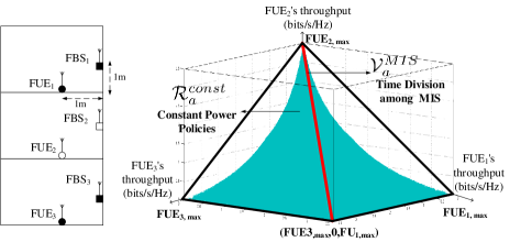
Figure 3: An example to illustrate the optimality of proposed framework.

V-D Complexity for computing the policy

We only compare the computational complexity of the proposed policies against cyclic MIS-based TDMA policies, since determining the optimal constant power based policy is a non-convex problem and has been shown to be NP-hard [34]. We compare the two for a given interference graph $G_{D}$. Both the optimal cyclic MIS TDMA and the proposed policy need to compute the set of MISs. Determining all the MISs in general requires large computational cost[3]. However, the computational complexity is acceptable if the network is small, or if the number of MIS, $s(G_{D})=\mathcal{O}((N+M)^{c}),\;c>1$ is bounded by a polynomial function in the number of vertices in $G_{D}$. We will develop an approximate algorithm to compute only a subset of MISs within polynomial time and with performance guarantees in Section VI. In our framework, the remaining amount of computation (other than computing MISs) is dominated by the amount of computation performed in Step 4, because in Step 5, the policy is computed online with a small amount $\mathcal{O}(s(G_{D}))$ of computations per time slot. In Step 4, we solve the optimization problem in (5) with the objective function $W$ and linear constraints. When $W$ is linear (e.g. weighted sum throughput) or is the minimum throughput of any UE (in which case the problem can be transformed into a linear programming), the worst-case computational complexity for solving (5) is $\mathcal{O}((s(G_{D})+N+M)^{3.5}B^{2})$[37] where $B$ is the number of bits to encode a variable. In contrast, the complexity of computing the optimal cyclic MIS-based TDMA policy of cycle length $L$ scales by $[s(G_{D})]^{L}$. The complexity quickly becomes intractable when cycle lengths are moderately higher than $N+M$, which is usually needed for acceptable performance. In summary, the complexity of computing our policies is much lower than that of computing cyclic MIS-based TDMA policies.

V-E Impact of the density of femtocells and macrocells

The density of the network is defined as the average number of neighbors of a UE in the interference graph. To obtain sharp analytical results, we restrict our attention to a class of interference graphs with $N+M$ vertices and $H$ cliques of the same size. Note that a clique is a subset of vertices, where any two vertices are connected. Assuming that no two cliques are connected, we can compute the density as $d=\frac{{N+M}}{H}-1$. When the total number $N+M$ of UEs remains the same and the density $d$ increases, the number $H$ of cliques will decrease. Since the vertices in a MIS can only come from different cliques, the number of MISs decreases as $H$ decreases. As a result, the complexity of the policy will decrease. When the density increases, the multi-user interference increases, leading to a decrease in the throughput and in the network performance.

VI Efficient Interference Management With Provable Performance Guarantees for Large-Scale Networks

VI-A Efficient Computation of A Subset of MISs

In our design framework proposed in Section V, we require the designer to compute all the MISs in Step 2. However, computing all the MISs is in general computationally prohibitive for large networks. We propose an approximate algorithm to compute a subset of MISs for a given interference graph $G_{D}$ in polynomial time and provide performance guarantees for our algorithm. Note that the graph $G_{D}$ belongs to the class of unit-disk graphs [38].

The subset of MISs are computed as follows.

i). Approximate Vertex Coloring: The designer first colors the vertices of interference graph $G_{D}$ using the approximate minimum vertex coloring scheme in [38]. Let $\mathcal{C}_{1}=\{1,...,C(G_{D})\}$ be the indices of the colors. It is proven in [38] that the number of colors used is bounded by $C^{*}(G_{D})\leq C(G_{D})\leq 3C^{*}(G_{D})\;\text{where}\;C^{*}(G_{D})\;$is the minimum number of colors that can be used to color the vertices of $G_{D}$.

ii). Generating MISs in a Greedy Manner: Each color $i$ corresponds to an independent set $I_{i}^{{}^{\prime}}$. For each independent set $I_{i}^{{}^{\prime}}$, the designer adds vertices in a greedy fashion until the set is maximally independent. The procedure is described in Table 3. Let the output MIS obtained from Table 3 be $I_{k(i)}^{G_{D}}$, where $k(i)$ is the index of the MIS in the original set of MISs  $\textbf{I}^{G_{D}}$. We write all the MISs augmented from $I_{i}^{{}^{\prime}},\,i=1,\ldots,C(G_{D})$ as $\{I_{k(1)}^{G_{D}},...I_{k(C(G_{D}))}^{G_{D}}\}.$

iii). $\textit{Generating the Approximate Maximum Weighted MIS}:$ Define a weight corresponding to each UE/vertex $i$ as $\bar{w_{i}}=r_{i}^{max}$, where $r_{i}^{max}$ is the maximum throughput achievable by UE $i$ when all the other UEs do not transmit. Given these weights, the designer ideally will like to find the maximum weighted MIS,  namely the MIS with the maximum sum weight of its vertices. However, finding the maximum weighted MIS is NP-hard [39]. Hence, the designer will find the $\eta$-approximate maximum weighted MIS, denoted $I_{k(C(G_{D})+1)}^{G_{D}}$, using the algorithm in [40].

The set of MISs computed from the above steps is then $\textbf{I}_{approx}^{G_{D}}=\{I_{k(1)}^{G_{D}},...I_{k(C(G_{D})+1)}^{G_{D}}\}$. Note that $\{I_{k(1)}^{G_{D}},...I_{k(C(G_{D}))}^{G_{D}}\}$ ensure that all the UEs are included in the scheduled MISs, and $I_{k(C(G_{D})+1)}^{G_{D}}$ is included for performance improvement. Given this subset of MISs, we can define $\mathcal{P}_{approx}^{MIS(G_{D})}=[\textbf{p}^{I_{k(1)}^{G_{D}}},...,\textbf{p}^{I_{k(C(G_{D})+1)}^{G_{D}}}]$, $\mathcal{R}_{approx}^{MIS(G_{D})}=\{\textbf{r}(\textbf{p}),\;\textbf{p}\in\mathcal{P}_{approx}^{MIS(G_{D})}\}$ and $\mathcal{V}_{approx}^{MIS(G_{D})}=\text{conv}\{\mathcal{R}_{approx}^{MIS(G_{D})}\}$. Let $\Pi_{approx}(G_{D})=\{\boldsymbol{\pi}:\mathbb{Z}_{+}\rightarrow\mathcal{P}_{approx}^{MIS(G_{D})}\}$ be the set of policies in which only the subset of MISs are scheduled. Steps 3,4 and 5 of the design framework in Section V are performed given this subset (See Fig. 2). The results of Theorem 1 and 2 still apply to the policies in $\Pi_{approx}(G_{D})$ and the set of achievable throughput profiles is $\mathcal{V}_{approx}^{MIS(G_{D})}$ given the $\delta\geq 1-\frac{1}{C(G_{D})+1}$ (See Corollary 1 and 2 in Appendix at the end). The target vector in $\mathcal{V}_{approx}^{MIS(G_{D})}$ and the corresponding coefficient is computed as in Step 4 of Section V and is denoted as $\textbf{y}_{approx}^{*}(G_{D})$, $\boldsymbol{\alpha}_{approx}^{*}(G_{D})$ respectively. The coefficient vector $\boldsymbol{\alpha}_{approx}^{*}(G_{D})$ along with the indices of the MISs that UE $i$ belongs to is transmitted to the BS $i$ as in the Step 5 of Section V.

The main intuition for the procedure developed above is as follows. Steps i) and ii) find MISs that contain all the UEs, and hence ensure that the minimum throughput requirements are satisfied. Step iii) finds the MIS that contains UEs with higher weights to optimize performance. Given the MISs obtained in Steps i)-iii) the Steps 3-5 of the design framework are performed.

Require: Target weights $\boldsymbol{\alpha}^{*}(G)=[\alpha_{1}^{*}(G_{D}),....,\alpha_{s(G_{D})}^{*}(G_{D})]$

Initialization: Sets $t=0$, $\alpha_{j}=\alpha_{j}^{*}$ for all $j\in\{1,...,s(G_{D})\}$.

repeat

Finds the MIS with the maximum weight

$r^{*}=\arg\max_{j\in\{1,..,s(G_{D})\}}\alpha_{j}$

if $i\in I_{r^{*}}^{G_{D}}$ then

Transmits at power level $p_{i}^{t}=p_{i}^{max}$

end if

Updates $\alpha_{j}$ for all $j\in\{1,...,s(G_{D})\}$ as follows

$\alpha_{r^{*}}=\frac{\alpha_{r^{*}}-(1-\delta)}{\delta}$,

$\alpha_{j}=\frac{\alpha_{j}}{\delta}$ $\forall j\not=r^{*}$

$t\leftarrow t+1$

until $\varnothing$

Table II: Algorithm run by each UE

Require: $V=\{1,..,N+M\}$ set of vertices, $\bar{w}$

vector of weights of vertices, Independent set $I_{i}^{{}^{\prime}}$ and

$\text{Adj}(I_{i}^{{}^{\prime}})$ where Adj(X) is the set of neighbors of $X$

Initialization: $I_{k(i)}^{G_{D}}=I_{i}^{{}^{\prime}}$, $\mathcal{N}_{i}^{{}^{\prime}}=V\cap(I_{i}^{{}^{\prime}}\cup\text{Adj}(I_{i}^{{}^{\prime}}))^{c}$,

here $(X)^{c}$ is the complement of $X$

While( $\mathcal{N}_{i}^{{}^{\prime}}\neq\phi$)

$\mathcal{N}_{i}^{{}^{\prime}}=\text{sort}(\mathcal{N}_{i}^{{}^{\prime}})$ , sort the vertices

in $\mathcal{N}_{i}^{{}^{\prime}}$ in the decreasing order of the weights $\bar{w}_{j}$

$v^{{}^{\prime}}=\mathcal{N}_{i,1}^{{}^{\prime}}$ , here $\mathcal{N}_{i,1}^{{}^{\prime}}$ is the first vertex in $\mathcal{N}_{i}^{{}^{\prime}}$

$I_{k(i)}^{G_{D}}=I_{k(i)}^{G_{D}}\cup v^{{}^{\prime}}$

$\mathcal{N}_{i}^{{}^{\prime}}=\mathcal{N}_{i}^{{}^{\prime}}\cap(\{v^{{}^{\prime}}\}\cup\text{Adj}(\{v^{{}^{\prime}}\})^{c}$

end

Table III: Algorithm run by the designer

VI-B Performance Guarantees for Large Networks

In this subsection, we consider the network performance criterion as the weighted sum throughput, and give performance guarantees for the policy when we compute the subset of MISs by Steps i)-iii) in the Subsection VI-A. Note that as we will show in the Section VII, the subset of MISs perform well in large networks for other network performance metrics as well. In particular the performance guarantee implies that the performance scales with the optimum $W(\textbf{y}^{*}(G_{D}))$ as the network size $N+M$ increases. Define $D_{ij}^{UE}$ as the distance from UE-$i$ to BS-$j$. We make the following homogeneity assumption, $p_{i}^{max}=p^{max}$, $\sigma_{i}^{2}=\sigma^{2}$, $R_{i}^{min}=R^{min}$, $\max_{i}D_{ii}^{UE}\leq\Delta$ and $w_{i}=\frac{1}{N+M}$ . Here $\Delta$ is fixed and does not depend on the size of the network. We fix these parameters in order to understand the performance guarantee as a function of the network size. Let the channel gain $g_{ij}=\frac{1}{(D_{ij}^{UE})^{np}}$, where $np$ is the path loss coefficient.

We choose the trade-off variables $\rho,\zeta,\kappa$ that satisfy $\rho+1<\min\{\frac{\log_{2}(1+\frac{p^{max}}{\Delta^{np}2^{\zeta}\sigma^{2}})}{3R^{min}},\frac{\kappa}{\zeta(1+\eta)}\log_{2}(1+\frac{p^{max}}{\Delta^{np}\sigma^{2}})\}$ and $0<\kappa<1$. Any eligible triplet $\rho,\zeta,\kappa$ will define a class of interference graphs that exhibit $\zeta$-WNI and have maximum degrees upper bounded by $\rho$. Note that such interference graphs can have arbitrarily large sizes (see the example at the end of this subsection). Then the following theorem provides performance guarantees for the policy described in Subsection VI-A for this class of interference graphs.

Theorem 4: For any interference graph that has a maximum degree no larger than $\rho$ and exhibits $\zeta$-WNI with $\rho+1<\min\{\frac{\log_{2}(1+\frac{p^{max}}{\Delta^{np}2^{\zeta}\sigma^{2}})}{3R^{min}},\frac{\kappa}{\zeta(1+\eta)}\log_{2}(1+\frac{p^{max}}{\Delta^{np}\sigma^{2}})\}$ the policy in Subsection VI-A achieves a performance $\textbf{W(y}_{approx}^{*}(G_{D}))$ with a guarantee that $\textbf{W(y}_{approx}^{*}(G_{D}))\geq\frac{(1-\gamma)(1-\kappa)}{(1+\eta)}\cdot\textbf{W(y}^{*}(G_{D}))$, where $\gamma=(3(\rho+1))\frac{R^{min}}{\log_{2}(1+\frac{p^{max}}{\Delta^{np}2^{\zeta}\sigma^{2}})}$.

See the Appendix at the end for the detailed proof.

Proof Sketch: The condition that the graph does not have a degree more than $\rho<\frac{\log_{2}(1+\frac{p^{max}}{\Delta^{np}2^{\zeta}\sigma^{2}})}{3R^{min}}-1$and the $\zeta$-WNI condition ensure that the algorithm proposed in Subsection VI-A yields a feasible solution satisfying each UE’s minimum throughput constraint. Also, it is shown that the minimum coefficient/fraction of time allocated to $I_{k(C(G_{D})+1)}^{G_{D}}$is $\alpha_{approx,k(C(G_{D})+1)}\geq(1-\gamma$). Then it is shown that if UEs in $I_{k(C(G_{D})+1)}^{G_{D}}$ were to transmit all the time then the competitive ratio achieved is no smaller than $\frac{1-\kappa}{(1+\eta)}$ . This combined with minimum coefficient of $I_{k(C(G_{D})+1)}^{G_{D}}$ leads to the competitive ratio guarantee of no less than $\frac{(1-\gamma)(1-\kappa)}{(1+\eta)}$.

The trade-off variables $\rho,\zeta,\kappa$ as their name suggests provide trade-offs between how large is the class of interference graphs for which we can provide performance guarantees, and how good are the competitive ratio guarantees. On one hand, a higher $\kappa$ allows higher $\rho$, and higher $\rho$ and $\zeta$ allow a larger class of graphs. On the other hand, as we can see from Theorem 4, higher $\rho$ and $\zeta$, provided that they are eligible (higher $\zeta$ decrease the maximum eligible $\rho$), result in higher $\gamma$, and higher $\gamma$ and $\kappa$ give lower competitive ratio guarantees. Hence, we can tune the design parameters to provide different levels of competitive ratio guarantees for different classes of interference graphs. Next, we give an example to illustrate Theorem 4.

Example: Consider a layout of FBSs in a $K\times K$ square grid, i.e. $K^{2}$ FBSs with a distance of $5$m between the nearest FBSs, and assume that each FUE is located vertically below its FBS at a distance of $1$ m. Fix the parameters $p^{max}=100$ mW, $\sigma^{2}=3$ mW, $R^{min}=0.1$bits/s/Hz, $\eta=0.1$, $np=4$ and the threshold $D=7$ m, which gives us the upper bound $\rho=4$ on the maximum degrees. We can also verify that the interference graphs under any number $K^{2}$ of FBSs exhibit $\zeta$-WNI with $\zeta=0.15$. Given $\rho=4$ and $\zeta=0.15$, we choose the minimum $\kappa=0.17$, which provides the highest competitive ratio guarantee of $0.53$. This performance guarantee holds for any interference graph of any size $K$.

To construct an efficient interference graph similar to Subsection V-B when the number of MISs are large, the designer must use the low complexity framework in Subsection VI-A. In this case the designer computes the subset of MISs as described in Subsection VI-A and compares the optimal solution obtained to decide the best threshold . Formally stated, the designer computes $G_{D_{approx}^{*}}=\text{arg}\max_{G\in\mathcal{G}}W(\textbf{y}_{approx}^{*}(G))$. See Fig. 2. for a comparison of the design framework in Subsection VI-A for large networks with that in Subsection V-A for small networks.

VI-C Complexity for computing the Subset of MISs

We show that the proposed approximation method for computing the subset of MISs described in Subsection VI-A has a complexity bounded by a polynomial in the number of vertices, i.e., $\mathcal{O}((N+M)^{c}),\;c>1$. This is because Steps i). and iii) use the algorithms developed in [38] and [40] for which the complexity has been proven to be polynomial and ii). uses a greedy strategy in which there can be a maximum of $N+M$ iterations since atleast one vertex is always removed from $\mathcal{N}_{i}^{{}^{\prime}}$ in each iteration. The worst possible number of computations in an iteration is bounded by $(N+M)^{2}$. Hence the upper bound of the complexity of Step ii). $\mathcal{O}((N+M)^{3}$). Hence, the subsets of the MISs can be computed within polynomial time, and the policy computed using this subset can guarantee a constant competitive ratio as shown in Subsection VI-B.

.

VI-D Extensions

VI-D1 Construction of interference graphs based on other rules

Our design frameworks in Section V-A and Section VI-A do not rely on a specific method for constructing the interference graph. In Step 2 of the design frameworks (i.e., the step in which the interference graph is constructed), we can replace our distance-based construction of the interference graph with construction based on other criteria, such as SINR, interference levels [22], etc. Then we can use the resulting interference graph as the input to Step 3. For construction rules based on other criteria, we can also use the procedure described in Section V-B to optimize the construction rule (e.g., to choose the optimal threshold of SINR or the interference level, above which an edge is drawn between two nodes).

Note that in the design framework in Section VI, we find a subset of MISs, instead of all MISs, because the network is large. To find this subset, we use the coloring algorithm in [40], which is known to have polynomial-time complexity for unit-disk graphs. This is where we used the fact that the interference graph is constructed based on distances (such that the resulting graph is a unit-disk graph). However, we can use other polynomial-time coloring algorithms if the interference graph is generated based on other criteria. We can use a standard greedy coloring algorithm as in [41]. In the next step we extend the ISs obtained by coloring to MISs. We can do this based on Step ii) in Section VI-A. The target weights and the corresponding schedule for these MISs can be generated based on Section VI-A. Results about the performance guarantees in terms of competitive ratio (See Theorem 4) can also be extended to this case.

VI-D2 Incorporating uncertainty in channel gains

Our design frameworks in Section V and Section VI can be extended to the deployment scenarios in which the channel gains are not static. For fast fading, we can replace the instantaneous throughput with the expected instantaneous throughput in our design frameworks. For slow fading, we can track the fading by regularly re-computing the policy. Re-computing the entire policy every time may be costly. In Section VII-C we show that the designer does not need to re-compute the entire policy to get considerable gains compared to the state-of-the-art. Specifically, the designer fixes the interference graph that is selected in the beginning, and only re-computes the target weights rather than re-compute the optimal interference graph and the corresponding target weights. We also show that the performance loss incurred with respect to the latter approach, which is based on an entire re-computation is limited (8%).

VI-D3 Incorporating beamforming

We focus on the case where each UE has one antenna. When UEs have multiple antennas, we can easily incorporate beamforming in our framework. Beamforming mitigates the interference among the UEs served by the same BS. Hence, we can remove the edges between UEs in the same cell from the interference graph. Then we can use the new interference graph as the input to Step 3 of our design framework.

VII Illustrative Results

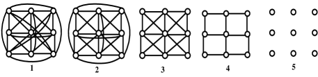
Fig. 4 a)

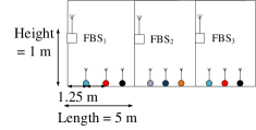
Fig. 4 b)

Figure 4: a) Different interference graphs for the 3 x 3 BS grid, b) Illustration of setup with 3 rooms.

In this section, we show via simulations that our proposed policy significantly outperforms existing interference management policies under different performance criteria. These performance gains are obtained under varying interference levels for both small and large networks. We also evaluate the proposed policy when the channel conditions are time-varying due to fading. In this case, the designer ideally needs to re-compute the optimal interference graph each time the channels change at the cost of a higher complexity. We show the robustness of the proposed policy when we choose a fixed interference graph regardless of the time-varying fading.

In each setting, we compare with the state-of-the-art policies described in Section II, namely the constant power control based policies and the cyclic MIS TDMA based policies. We do not compare with coloring based TDMA/Frequency reuse policies as it was already shown in Subsection IV-B that the MIS based TDMA policies will always lead to better network performance. Throughout this section, we will set the discount factor as the minimum one required when we use our original design framework in Section V (namely $\delta=1-\frac{1}{s(G_{D})}$ according to Theorems 1-2), and the minimum one required when we use the approximate design framework for large networks in Section VI (namely $\delta=1-\frac{1}{C(G_{D})+1}$). In this way, we evaluate the performance of our proposed policies under the most delay-sensitive applications.

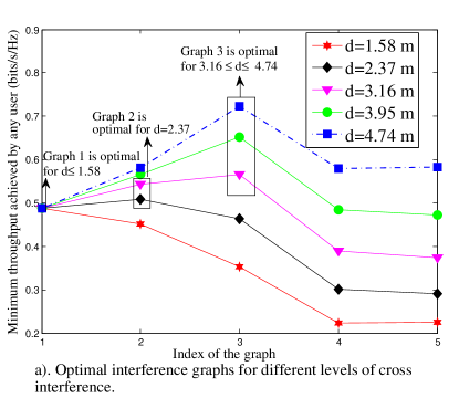
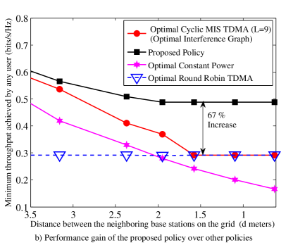
Figure 5: a) Optimal interference graph selection for 3 x 3 grid. b) Performance comparison of the proposed policy for different size of the grid.

VII-A Performance Gains Under Varying Interference Levels

Consider a $3\text{x}3$ square grid of 9 BSs and corresponding UEs with the minimum distance between any two BSs given as $d$ (see Fig. 4 a.). Each UE $i$ has $\delta=0.89$ and a maximum power of $200$ mW. Assume that the UEs an the BSs are in two horizontal hyperplanes, and each BS is vertically above its UE with a distance of $3.16m$. Then the distance from UE $i$ to another BS $j$ is $D_{ij}^{UE}=\sqrt{3.16^{2}+(D_{ij}^{BS})^{2}}$ , where $D_{ij}^{BS}$ is the distance between BSs $i$ and $j$. The channel gain from UE $i$ to BS $j$ is $g_{ij}=\frac{1}{(D_{ij}^{UE})^{2}}$. The performance criterion is the max-min fairness. Under different thresholds $D$ chosen by the designer, there are 5 possible topologies of the interference graph, as shown in the Fig. 4 a. For each grid size $d$, the optimal solution to (2) is computed for each interference graph as described in Subsection V-B. Fig. 5 a). shows that under different grid sizes (i.e. different interference levels), the optimal interference graph (i.e. the optimal threshold) changes. As the interference level increases, the corresponding optimal interference graph has more edges. Fig. 5 b). compare the performances of different policies under different grid sizes $d$ (i.e. different interference levels), where the interference graph is the optimal one. We can see that the proposed policy achieves up to 67$\%$ performance gain over the second best policy. Through the above results, we see that 1) it is important to construct different interference graphs based on the interference level, and 2) the proposed non-stationary schedule of MISs outperform the cyclic schedules.

VII-B Performance Scaling in Large Networks

We study a dense deployment scenario to evaluate the performance gain of our proposed scheme over the state-of-the-art. We allow more than one UE to transmit to a single BS, and will increase the number of UEs associated with a BS. Consider the uplink of a femtocell network in a building with 12 rooms adjacent to each other. Fig. 4 b). illustrates 3 of the 12 rooms with 3 UEs in each room. For simplicity, we consider a 2-dimensional geometry, in which the rooms and the FUEs are located on a line. Each room has a length of 6 meters. In each room, there are $P$ uniformly spaced FUEs, and one FBS installed on the left wall of the room at a height of 2m. The distance from the left wall to the first FUE, as well as the distance between two adjacent FUEs in a room, is $\frac{6}{(1+P)}$ meters. Based on the path loss model in [36], the channel gain from each FBS $i$ to a FUE $j$ is $\frac{1}{(D_{ij}^{UE})^{2}\Delta^{n_{ij}}}$, where $\Delta=10^{0.25}$ is the coefficient representing the loss from the wall, and $n_{ij}$ is the number of walls between FUE $i$ and FBS $j$. Each UE has a maximum transmit power level of $1000$ mW and a minimum throughput requirement of $R_{i}^{min}=0.05$ bits/s/Hz. For each $P$, the designer chooses the optimal threshold to construct the optimal interference graph. Note that the UEs in the same room accessing the same BSs are all connected to each other in the interference graph, since the distances between their receiving BSs is $0$.

We vary the number $P$ of FUEs in each room from $5$ to $15$. We fix the $\delta=0.97$ , i.e. the least value it can take based on the largest number of UEs per room, i.e. $P=15$. For each $P$, the designer constructs the optimal graph G as described in Subsection VI-A using the low complexity method as the number of UEs is large. Under all considered values of $P$, the optimal interference graph connects all the UEs in adjacent rooms with edges and does not connect the UEs in non-adjacent rooms. We use the same optimal graph to compute the optimal cyclic MIS TDMA of cycle length L. The cycle length is varied from $12$ to $58$ depending upon the number of UEs (we try to choose as large cycle lengths as possible to maximize performance within a feasible computational complexity). The number of non-trivial cyclic policies under different $P$ may vary from $10^{8}$ to even more than $10^{50}$ which renders exhaustive search to be intractable. Hence, for each $P$ we do a randomized search in $4$ million policies to search for the optimal one. Fig. 6. compares the performance of different policies in terms of both the max-min fairness and the sum throughput. The constant power policy cannot satisfy the feasibility conditions for any number of UEs in each room. The performance gain over cyclic MIS TDMA policies increases as the network becomes larger. When there are 15 UEs in each room, we can improve the worst UE’s throughput by $131\%$ compared to cyclic MIS TDMA policies.

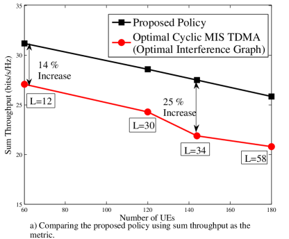
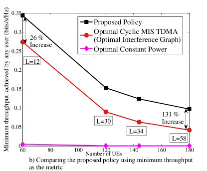
Figure 6: Comparing the proposed policy against others for a) sum throughput as the metric, b) minimum throughput as the metric.

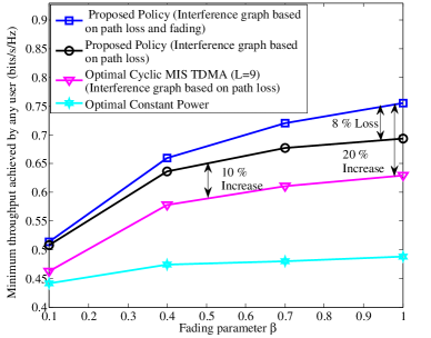
Figure 7: Illustrating the robustness of interference graph selection based on path loss.

VII-C Performance under Dynamic Channel Conditions

We consider a 9-cell network with a grid size $d=4.74$ m, where each BS is vertically above its UE at a distance of $3.16$ m as in Subsection VII-A. Each UE has a maximum power level of 1000 mW, noise power of 1 mW and $\delta=0.89$. The channel gain is the product of path loss as in Subsection VII-A and fading component, $f_{ij}\sim Rayleigh(\beta)$ . Here, we assume that the fading component changes every $50$ time slots independently and the new channel conditions are reported to the designer by each FBS as in Step-1 in Subsection V-A. The designer has the choice of re-computing the optimal interference graph and thereby the optimal target every 50 time slots at the cost of a higher complexity, or choosing a fixed optimal interference graph based on the channel gains computed from the path loss model (which will be graph 3 in Fig. 4 a) and selecting the optimal target every 50 time slots based on it. In Fig. 7 we compare the loss due to choosing a fixed interference graph with choosing the optimal interference graph every 50 time slots. We average the performance for a duration over a total of 10000 time slots for a fixed $\beta$. In Fig. 7, we see that for a low $\beta$, i.e. $\beta=0.1$ which implies a lower variance in fading the loss is only $1$% and even when $\beta$ is large, i.e. $\beta=1$ then as well the loss is $8$%. We also compare with Cyclic MIS TDMA , cycle length $L=9$ and optimal constant power policy, the performance gain with the proposed policy using a fixed interference graph is consistently 10 $\%$ for varying fading conditions $\beta$, while choosing the optimal interference graph can lead to a maximum gain of $20$%.

VIII Conclusion

In this work, we proposed a novel and systematic method for designing efficient interference management policies in a network of macrocell underlaid with femtocells. The proposed framework relies on constructing optimal interference graphs and optimally scheduling the MIS of the constructed graph to maximize the network performance given the minimum throughput requirements. Importantly, the proposed policy is non-stationary and can address the requirements of delay sensitive users. We prove the optimality of the proposed policies under various deployment scenarios. The proposed policy can be implemented in a decentralized manner with low overhead of information exchange between BSs and UEs. For large networks, we develop a low-complexity design framework that is provably efficient. Our proposed policies achieve significant (up to 130 $\%$) performance improvement over existing policies, especially for dense and large-scale deployments of femtocells.

IX Appendix

We would begin by defining a self-generating set similar to what is defined in repeated game theory [42]. However, our definition is less restrictive since it does not involve incentive compatibility as required in strategic user setting in repeated games.

Definition 1. Decomposability : A throughput vector $\textbf{v}\in\mathbb{R}^{N+M}$ is decomposable on a set $\mathcal{W}$ with respect to a discount factor $\delta$, if there exists a power profile $\textbf{p}\in\mathcal{P}^{MIS(G_{D})}$ and a mapping $\boldsymbol{\gamma}:\mathcal{P}^{MIS(G_{D})}\rightarrow\mathcal{W}$ such that $\forall i\;\in\{1,...N+M\}$

$$v_{i}=(1-\delta)r_{i}(\textbf{p})+\delta\gamma_{i}(\textbf{p})$$ (3)

Define $\mathcal{D}(\mathcal{W},\delta)=\{\textbf{v}:\textbf{v}\text{\;\ is pure action decomposable on\;}\mathcal{W}\}$.

Definition 2. Self-Generation : $\mathcal{W}$ is self-generating with respect to discount factor $\delta$, if each throughput vector $\textbf{v}\in\mathcal{W}$ is decomposable on $\mathcal{W}$, thus $\mathcal{W}\subseteq\mathcal{D}(\mathcal{W},\delta)$

Theorem 1: Given the interference graph $G_{D}$, for any $\delta\geq\bar{\delta}=1-\frac{1}{s(G_{D})}$, the set of throughput profiles achieved by MIS-based policies is $\mathcal{V}^{MIS(G_{D})}(\delta)=\mathcal{V}^{MIS(G_{D})}$.

Proof: $\mathcal{V}^{MIS(G_{D})}=\text{conv}\{\mathcal{R}^{MIS(G_{D})}\}$, where $\mathcal{R}^{MIS(G_{D})}=\{\textbf{r}(\textbf{p}^{I_{j}^{G_{D}}}),\forall j\in\{1,...,s(G_{D})\}\}$ and $\text{conv}\{X\}$ is the convex hull of the set $X$. We will show that $\mathcal{V}^{MIS(G_{D})}$ is self-generating for $\delta\geq\bar{\delta}$. If we can show that the set is self-generating then we can contruct an MIS-based policy which achieves any given target vector in that set. This is explained as follows. Let us assume that $\mathcal{V}^{MIS(G_{D})}$ is self-generating with respect to certain $\delta$, then given a vector $\textbf{v}\in\mathcal{V}^{MIS(G_{D})}$ it can be decomposed as, $\textbf{v}=(1-\delta)\textbf{r}(\textbf{p}^{I_{j}^{G_{D}}})+\delta\boldsymbol{\gamma}(\textbf{p}^{I_{j}^{G_{D}}})$. The vector $\boldsymbol{\gamma}(\textbf{p}^{I_{j}^{G_{D}}})$ obtained on decomposition is treated as the target vector for the transmissions starting the next period. We know that $\boldsymbol{\gamma}(\textbf{p}^{I_{j}^{G_{D}}})\in\mathcal{V}^{MIS(G_{D})}$ and $\mathcal{V}^{MIS(G_{D})}$ is assumed to be self-generating, which means $\boldsymbol{\gamma}(\textbf{p}^{I_{j}^{G_{D}}})$ can also be decomposed in the same manner by a certain MIS based power profile $\textbf{p}^{I_{j}^{G_{D}}}\in\mathcal{R}^{MIS(G_{D})}$. This step can be recursively followed for all the future periods to generate a policy and hence, the target v is achieved. Next, we show the conditions under which the set $\mathcal{V}^{MIS(G_{D})}$ is indeed self-generating.

Let $\textbf{v}\in\mathcal{V}^{MIS(G_{D})}$ and we can express $\textbf{v}=\sum_{k=1}^{s(G_{D})}\alpha_{k}\textbf{r}(\textbf{p}^{I_{k}^{G_{D}}}),\;\alpha_{k}\geq 0,\;\forall k\in\{1,....,s(G_{D})\}\;\text{and }$

$\sum_{k=1}^{s(G_{D})}\alpha_{k}=1$. If $\mathcal{V}^{MIS(G_{D})}$ is self-generating with respect to certain discount factor $\delta$ then $\exists\;\textbf{p}^{I_{j}^{G_{D}}}\;\text{and}\;\boldsymbol{\gamma}(\textbf{p}^{I_{j}})\in\mathcal{V}^{MIS(G_{D})}$ about which v can be decomposed as follows

$$\textbf{v}=(1-\delta)\textbf{r}(\textbf{p}^{I_{j}^{G_{D}}})+\delta\boldsymbol{\gamma}(\textbf{p}^{I_{j}^{G_{D}}})$$ (4)

Next, we come up with sufficient conditions for $\boldsymbol{\gamma}(\textbf{p}^{I_{j}^{G_{D}}})\in\mathcal{V}^{MIS(G_{D})}$

$$\boldsymbol{\gamma}(\textbf{p}^{I_{j}^{G_{D}}})=\frac{\textbf{v}-(1-\delta)\textbf{r}(\textbf{p}^{I_{j}^{G_{D}}})}{\delta}$$

$$=\sum_{k=1,k\not=j}^{s}\frac{\alpha_{k}}{\delta}\textbf{r}(\textbf{p}^{I_{k}^{G_{D}}})+\frac{\alpha_{j}-(1-\delta)}{\delta}\textbf{r}(\textbf{p}^{I_{j}^{G_{D}}})$$

Observe that $\sum_{k=1}^{s}\frac{\alpha_{k}}{\delta}+\frac{\alpha_{j}-(1-\delta)}{\delta}=1$. If $0\leq\frac{\alpha_{k}}{\delta}\leq 1,\forall k\in\{1,...,s(G_{D})\},k\not=j$ and $0\leq\frac{\alpha_{j}-(1-\delta)}{\delta}\leq 1$ then $\boldsymbol{\gamma}(\textbf{p}^{I_{j}^{G_{D}}})\in\mathcal{V}^{MIS(G_{D})}$. This can be combined into one condition on $\delta$ given as

$$\delta\geq\{\max_{k\not=j}\{\alpha_{k}\},1-\alpha_{j}\}$$

Note that decomposition condition requires for the existence of atleast one profile $\textbf{p}^{I_{j}^{G_{D}}}$. This means we can choose the least possible bound on $\delta$, which is sufficient to ensure that there will exist at least one profile $\textbf{p}^{I_{j}^{G_{D}}}$for decomposition.

$$\delta \geq\min_{j\in\{1,..s(G_{D})\}}\{\max_{k\not=j}\{\alpha_{k}\},1-\alpha_{j}\},$$

$$=1-\alpha_{[s(G_{D})]},$$

where $\alpha_{[s(G_{D})]}=\max_{j\in\{1,...,s(G_{D})\}}\{\alpha_{1},...,\alpha_{s(G_{D})}\}$. Also, $\sum_{k=1}^{s(G_{D})}\alpha_{k}=1,\;\alpha_{k}\geq 0,\;\forall k\in\{1,...,s(G_{D})\}$ yields that $\alpha_{[s(G_{D})]}\geq\frac{1}{s(G_{D})}$. Hence, the condition $\delta\geq 1-\frac{1}{s(G_{D})}$ is sufficient to ensure decomposition of every vector in the convex hull. Thus, $\mathcal{V}^{MIS(G_{D})}$ is self-generating for all the discount factors $\delta\geq\bar{\delta}=1-\frac{1}{s(G_{D})}$. Hence, we have been able to show that for a discount factor $\delta\geq 1-\frac{1}{s(G_{D})}$ each vector in $\mathcal{V}^{MIS(G_{D})}$ can be achieved by an MIS based policy, i.e. $\mathcal{V}^{MIS(G_{D})}\subseteq\mathcal{V}^{MIS(G_{D})}(\delta)$. The throughput achieved by any MIS based policy is $\boldsymbol{R}(\boldsymbol{\pi})=(1-\delta)\sum_{t=0}^{\infty}\delta^{t}\textbf{r}(\boldsymbol{p}^{t})$, here $\textbf{r}(\boldsymbol{p}^{t})\in\mathcal{R}^{MIS(G_{D})}$. Since the coefficients $(1-\delta)\delta^{t}\geq 0$ and the sum of the coefficients of the throughput vector sum to 1, i.e. $\sum_{t=0}^{\infty}(1-\delta)\delta^{t}=1$, this implies $\boldsymbol{R}(\boldsymbol{\pi})\in\mathcal{V}^{MIS(G_{D})}$. Hence, $\mathcal{V}^{MIS(G_{D})}(\delta)\subseteq\mathcal{V}^{MIS(G_{D})}$. Therefore, $\mathcal{V}^{MIS(G_{D})}(\delta)=\mathcal{V}^{MIS(G_{D})}$ for $\delta\geq 1-\frac{1}{s(G_{D})}$. Next, we give a corollary of the above Theorem 1, which states the restriction on the discount factor and the corresponding achievable set for the policy based on the subset of MISs in Section VI.

(Q.E.D)

Corollary 1: Given the interference graph $G_{D}$, if the $\delta\geq 1-\frac{1}{C(G_{D})+1}$ then the throughput vectors achieved by the policies in $\Pi_{approx}^{MIS(G_{D})}$ is $\mathcal{V}_{approx}^{MIS(G_{D})}$.

Proof: This follows on the same lines as Theorem 1. $\mathcal{V}_{approx}^{MIS(G_{D})}=\text{conv}\{\mathcal{R}_{approx}^{MIS(G_{D})}\}$, where $\mathcal{R}_{approx}^{MIS(G_{D})}=\{\textbf{r}(\textbf{p}^{I_{j}^{G_{D}}}),\forall j\in\{k(1),...,k(C(G_{D})+1)\}\}$. It can be shown on the same lines that $\mathcal{V}_{approx}^{MIS(G_{D})}$ is self-generating if $\delta\geq 1-\frac{1}{C(G_{D})+1}$. This is due to the fact that $\mathcal{V}_{approx}^{MIS(G_{D})}$ has $C(G_{D})+1$ extreme points.

(Q.E.D)

Theorem 2: For any $\delta\geq\bar{\delta}=1-\frac{1}{s(G_{D})}$ the policy computed in Table 2 (given in Section V) achieves the target throughput $\textbf{y}^{*}(G_{D})$.

Proof: The policy in Table 2 (given in the paper) is based on the decomposition property of $\mathcal{V}^{MIS(G_{D})}$ (explained in the proof of Theorem 1). Define $\boldsymbol{\gamma}(t)=\sum\limits_{k=1}^{s(G_{D})}\alpha_{k}(t)\textbf{r}(\textbf{p}^{I_{k}^{G_{D}}})$, where $\alpha_{k}(t),\;\forall k\in\{1,...,s(G_{D})\},\;\forall\;t\geq 0$ correspond to the coefficient $\boldsymbol{\alpha}=(\alpha_{1},...,\alpha_{N+M})$ at the beginning of time slot $t$ in the policy in Table 2. Also, let $\textbf{p}^{I_{r_{t}}^{G_{D}}}$ correspond to the power vector used for transmission at time $t$ for $t\geq 0$. First, we show that if $\delta\geq\bar{\delta}$ then $\boldsymbol{\gamma}(t+1)\in\mathcal{V}^{MIS(G_{D})},\;\forall t\geq 0$. Expressing $\gamma(t+1)$ in terms of coefficients of $\alpha_{k}(t),\;\forall k\in\{1,..s(G_{D})\}$ as in Table 2.

$$\boldsymbol{\gamma}(t+1)=\sum_{k=1}^{s(G_{D})}\alpha_{k}(t+1)\textbf{r}(\textbf{p}^{I_{k}^{G_{D}}})=\sum\limits_{k=1,k\not=r_{t}}^{s(G_{D})}\frac{\alpha_{k}(t)}{\delta}\textbf{r}(\textbf{p}^{I_{k}^{G_{D}}})+\frac{\alpha_{r_{t}}(t)-(1-\delta)}{\delta}\textbf{r}(\textbf{p}^{I_{r_{t}}^{G_{D}}})$$ (5)

where $\alpha_{r_{t}}(t)=\max_{k}\alpha_{k}(t)$. If $0\leq\frac{\alpha_{k}(t)}{\delta}\leq 1,\forall k\in\{1,...,s(G_{D})\},k\not=r_{t}$ and $0\leq\frac{\alpha_{r_{t}}(t)-(1-\delta)}{\delta}\leq 1$ then $\boldsymbol{\gamma}(t+1)\in\mathcal{V}^{MIS(G_{D})}$. If $\delta\geq\max_{t\geq 0}1-\alpha_{r_{t}}(t)$ then $\bm{\gamma}(t+1)\in\mathcal{V}^{MIS(G_{D})}\,\forall t$. We know that $\alpha_{r_{t}}(t)\geq\frac{1}{s(G_{D})},\forall t$, this is true because $\alpha_{r_{t}}(t)=\max_{k}\alpha_{k}(t)$. The condition on $\delta\geq 1-\frac{1}{s(G_{D})}$ implies that $\boldsymbol{\gamma}(t+1)\in\mathcal{V}^{MIS(G_{D})}$,$\forall t\geq 0$. Therefore, we can express

$$\boldsymbol{\gamma}(t)=(1-\delta)\textbf{r}(\textbf{p}^{I_{r_{t}}^{G_{D}}})+\delta\boldsymbol{\gamma}(t+1)$$

here $\boldsymbol{\gamma}(t+1)\in\mathcal{V}^{MIS(G_{D})}$ . Hence using this recursively we get,

$$\boldsymbol{\gamma}(0)-(1-\delta)\sum\limits_{\tau=0}^{t}\delta^{\tau}\textbf{r}(\textbf{p}^{I_{r_{\tau}}^{G_{D}}})=\delta^{t+1}\boldsymbol{\gamma}(t+1)$$ (6)

Here, $\boldsymbol{\gamma}(t+1)\in\mathcal{V}^{MIS(G_{D})}$ and $\boldsymbol{\gamma}(0)=\textbf{y}^{*}(G_{D})$ The above expression in (4) specifies the difference from the target vector and the vector achieved till time $t$. Next, we find the time $T$ after which the norm of difference in 6 is below $\epsilon$. $\boldsymbol{\gamma}(t+1)$ can be bounded above (since $\mathcal{V}^{MIS(G_{D})}$is closed and bounded), $||\boldsymbol{\gamma}(t+1)||\leq\theta^{bd}$, $\forall t\geq 0$. Hence, $T=\frac{\log(\frac{\epsilon}{\theta^{bd}})}{\log(\delta)}-1$ is sufficiently high to ensure the norm of difference in 6 is below $\epsilon$. Hence as $\epsilon$ is chosen small, the policy would converge to the target payoff.

Next, we give a corollary, which states the condition on the policy based on the subset of the MISs computed in Subsection VI-A.

(Q.E.D)

Corollary 2: For any $\delta\geq 1-\frac{1}{C(G_{D})+1}$ the policy computed in Table 2 based on the subset of MISs computed in Subsection VI-A achieves the target throughput $\textbf{y}_{approx}^{*}(G_{D}))$

Proof: The policy in Table 2 using the target weights $\boldsymbol{\alpha}_{approx}^{*}(G_{D})$ is based on the decomposition property of $\mathcal{V}_{approx}^{MIS(G_{D})}$. Here also using the decomposition property repeatedly it can be shown that the difference between the target and the target vector achieved till time $t$ decreases exponentially which proves convergence.

Next, we state two lemmas which will be used to prove Theorem 3 and 4. Also, note that any inequality between two vectors would represent a component-wise inequality.

Lemma 1: In a bounded degree graph with $N+M$ vertices and bound on the maximum degree $\rho$ there exists a maximal independent set with size $\frac{N+M}{\rho+1}$

Proof: In a bounded degree graph the maximum chromatic number for the conventional vertex coloring is $\rho+1$ [41]. Let the independent sets corresponding to each color class obtained by using the minimum coloring with atmost $\rho+1$ colors be given as $\{I_{1}^{{}^{\prime}},....,I_{\rho+1}^{{}^{\prime}}\}$ and let the sets of the sizes corresponding to each of these independent sets be given as $\{n_{1},....,n_{\rho+1}\}$. Let the set of maximum size be $I_{[1]}^{{}^{\prime}}$ and the corresponding size be given as $n_{[1]}$. We know that $\sum_{i=1}^{\rho+1}n_{i}=N+M$ and $n_{[1]}\geq n_{i},\forall i\in\{1,...,\rho+1\}$. From these conditions we can obtain $(\rho+1)n_{[1]}\geq N+M$. Hence, $n_{[1]}\geq\frac{N+M}{\rho+1}$.

(Q.E.D)

Lemma 2: If the interference graph exhibits $\epsilon$-WNI then the expression $r_{i}^{{}^{\prime}}(\textbf{p})$ (as defined in Subsection V-C in the paper) is an $\epsilon$ approximation to the actual rate $r_{i}(\textbf{p})$ and this holds for all $i\in\{1,...,N+M\}$ and $\textbf{$\forall$\ p}\in\mathcal{P}$.

Proof: To show that $r_{i}^{{}^{\prime}}(\textbf{p})$ is an $\epsilon$ approximation, it is sufficient to show that $\max_{\textbf{p}\in\mathcal{P}}|e_{i}(\textbf{p})|\leq\epsilon$, where $e_{i}(\textbf{p})=r_{i}^{{}^{\prime}}(\textbf{p})-r_{i}(\textbf{p})$. Solving for $\text{arg}\max_{\textbf{p}\in\mathcal{P}}|e_{i}(\textbf{p})|$, we get $p_{i}=p_{i}^{max}$, $p_{j}=0,\;\forall j\;\in\mathcal{N}_{i}(G_{D})$ and $p_{k}=p_{k}^{max},\;\forall k\in(\mathcal{N}_{i}(G_{D})\cup\{i\})^{c}$. This is explained as follows. Since the accumulative interference from non-neighbors is not accounted for in $r_{i}^{{}^{\prime}}(\textbf{p})$ this means $r_{i}^{{}^{\prime}}(\textbf{p})\geq r_{i}(\textbf{p})\,\implies$ $e_{i}(\textbf{p})\geq 0,\forall\textbf{p}\in\mathcal{P}$. Note that $e_{i}(\textbf{p})=\log_{2}(\frac{1+\frac{g_{ii}p_{i}}{\sum_{j\in\mathcal{N}_{i}(G_{D})}g_{ji}p_{j}+\sigma_{i}^{2}}}{1+\frac{g_{ii}p_{i}}{\sum_{j\not=i}g_{ji}p_{j}+\sigma_{i}^{2}}})$ is an increasing function in $p_{i}$ and $p_{k},\;\forall k\in(\mathcal{N}_{i}(G_{D})\cup\{i\})^{c}$ and a decreasing function of $p_{j},\;\forall j\in\mathcal{N}_{i}(G_{D})$. From this we get that $e_{i}(\textbf{p})$ takes its maximum value when $p_{i}=p_{i}^{max}$ and $p_{k}=p_{k}^{max},\;\forall k\in(\mathcal{N}_{i}(G_{D})\cup\{i\})^{c}$ and $p_{j}=0,\;\forall j\in\mathcal{N}_{i}(G_{D})$. The corresponding maximum value is $e_{i}^{max}=\log_{2}(\frac{1+\frac{g_{ii}p_{i}^{max}}{\sigma^{2}}}{1+\frac{g_{ii}p_{i}^{max}}{\sum_{\forall k\in(\mathcal{N}_{i}(G_{D})\cup\{i\})^{c}}g_{ki}p_{k}^{max}+\sigma^{2}}})$. This combined with $\epsilon$-WNI, i.e. $Int_{i}^{max}(G_{D})=\sum_{k\in(\mathcal{N}_{i}(G_{D})\cup\{i\})^{c}}g_{ki}p_{j}^{max}\leq(2^{\epsilon}-1)\sigma_{i}^{2}$ gives that $e_{i}^{max}\leq\epsilon$. The same argument holds for any $i$.

(Q.E.D)

Theorem 3: If the constructed interference graph $G_{D^{*}}$ exhibits SLI and $\epsilon$-WNI, then the proposed policy computed through Steps 1-5 of Section V-A achieves within $\epsilon$ of the optimal network performance $W^{*}$.

Proof: With constraint tolerance of $\epsilon$, the optimization problem in Step 5 of the design framework is stated as follows.

$$\max_{\textbf{y},\boldsymbol{\alpha}}W(y_{1}(G_{D}),....,y_{N+M}(G_{D}))$$ (7)

$$y_{i}(G_{D})\geq R_{i}^{min}-\epsilon,\;\forall i\in\{1,...,N+M\}$$

$$y_{i}(G_{D})=\sum_{k=1}^{s(G_{D})}\alpha_{k}r_{i}(\textbf{p}^{I_{k}^{G_{D}}}),\;\forall i\in\{1,...,N+M\}$$

$$\alpha_{k}\geq 0,\forall k\in\{1,...s(G_{D})\}$$

$$\sum_{k=1}^{s(G_{D})}\alpha_{k}=1$$

The optimal argument of the above problem is $\textbf{y}^{*}(G_{D})$. Define $\textbf{y}^{*}(G_{D^{*}})=\text{arg}\max_{D\leq D_{max}^{BS}}W(\textbf{y}^{*}(G_{D}))$.

Consider the design problem in in Subsection IV-A (given in the paper). The feasible region for average throughput vectors for the design problem is a subset of $\text{conv}\{\mathcal{R}^{const}\}$. This is explained as follows. The throughput vector achieved by an interference management policy can be written as: $\textbf{R}(\boldsymbol{\pi})=(1-\delta)\sum_{t=0}^{\infty}\delta^{t}\textbf{r}(\textbf{p}^{t})$, here $\textbf{R}(\boldsymbol{\pi})=(R_{1}(\boldsymbol{\pi}),...,R_{N+M}(\boldsymbol{\pi}))$. The coefficients of $\textbf{r}(\textbf{p}^{t})$ are positive and the sum of these coefficients is 1 and $\textbf{r}(\textbf{p}^{t})\in\mathcal{R}^{const}$, which implies that $\textbf{R}(\boldsymbol{\pi})\in conv\{\mathcal{R}^{const}\}$. Let $\textbf{v}^{*}\in\text{conv}\{\mathcal{R}^{const}\}$ be the optimal solution to the design problem in Subsection IV-A (given in the paper) with weighted sum throughput as the objective and the corresponding optimal value of the objective is $W^{*}=\sum_{i=1}^{N+M}w_{i}v_{i}^{*}$, where $w_{i}\geq 0\;\forall i\in\{1,...,N+M\}$ and $\sum_{i=1}^{N+M}w_{i}=1$. Note that we have assumed that the design problem in Subsection IV-A is feasible, otherwise if it is not feasible then clearly the proposed framework will be infeasible as well. Expressing $\textbf{v}^{*}$ in terms of throughput vectors in $\mathcal{R}^{const}$ as follows, $\textbf{v}^{*}=\sum_{j=1}^{q}\theta_{j}\textbf{r}^{j,*}$ where $\textbf{r}^{j,*}\in\mathcal{R}^{const}$ , $\theta_{j}\geq 0,\;\forall j\in\{1,...,N+M\}$ and $\sum_{j=1}^{q}\theta_{j}=1$. Here, $\textbf{v}^{*}\geq\textbf{R}^{min}$ where $\textbf{R}^{min}=[R_{1}^{min},...,R_{N+M}^{min}]$ and the inequality between the vectors is a component-wise inequality. Our aim is to show that there exists $\textbf{v}\in\mathcal{V}^{MIS(G_{D^{*}})}$ which is $\epsilon$ close to the optimal and satisfies the minimum throughput constraint within a tolerance of $\epsilon$. Let $\textbf{r}(\textbf{p}^{j,*})=\textbf{r}^{j,*}$ and let $\textbf{r}^{{}^{\prime}}(\textbf{p}^{j,*})\in\mathcal{R}_{a}^{const}$ be the corresponding throughput taking only the interference from neighbors into account (given in Subsection V-C in the paper). Let $\tilde{\textbf{v}}\in conv\{\mathcal{R}_{a}^{const}\}$ defined as follows $\tilde{\textbf{v}}=\sum_{j=1}^{q}\theta_{j}\textbf{r}^{{}^{\prime}}(\textbf{p}^{j,*})$. Since $\textbf{r}^{{}^{\prime}}$ is computed only from the interference contribution of the neighbors we have $\textbf{r}^{{}^{\prime}}(\textbf{p}^{j,*})\geq\textbf{r}(\textbf{p}^{j,*})$ and from SLI we know that there exists $\textbf{v}^{{}^{\prime},j}\in\mathcal{V}_{a}^{MIS(G_{D^{*}})}$ which satisfies

$$\textbf{v}^{{}^{\prime},j}\geq\textbf{r}^{{}^{\prime}}(\textbf{p}^{j,*})\geq\textbf{r}(\textbf{p}^{j,*}),\forall j\in\{1,....,q\}$$ (8)

Let $\textbf{v}^{{}^{\prime}}=\sum_{j=1}^{q}\theta_{j}\textbf{v}^{{}^{\prime},j}$. Using above (8) we get,

$$\textbf{v}^{{}^{\prime}}\geq\tilde{\textbf{v}}\geq\textbf{v}^{*}$$ (9)

Expressing $\textbf{v}^{{}^{\prime},j}$ in terms of the throughput vectors in $\mathcal{R}_{a}^{MIS(G_{D^{*}})}$ we get $\textbf{v}^{{}^{\prime},j}=\sum_{k=1}^{s(G_{D^{*}})}\beta_{k}^{j}\textbf{r}^{{}^{\prime}}(\textbf{p}^{I_{k}^{G_{D^{*}}}})$ and the corresponding actual throughput is given as $\textbf{v}^{j}=\sum_{k=1}^{s(G_{D^{*}})}\beta_{k}^{j}\textbf{r}(\textbf{p}^{I_{k}^{G_{D^{*}}}})$. From the condition in the Theorem we know $G_{D^{*}}$ exhibits $\epsilon$-WNI which means $Int_{i}^{max}(G_{D^{*}})\leq(2^{\epsilon}-1)\sigma_{i}^{2}\;\forall i\;\in\{1,..,N+M\}$. Hence using Lemma 2, we have $r_{i}^{{}^{\prime}}(\textbf{p})$ is an $\epsilon$ approximation to $r_{i}(\textbf{p})$ and this holds for all $i\in\{1,...,N+M\}.$ Using $\textbf{r}(\textbf{p}^{I_{k}^{G_{D^{*}}}})\geq\textbf{r}^{{}^{\prime}}(\textbf{p}^{I_{k}^{G_{D^{*}}}})-\epsilon,\;\forall k\in\{1,..,s(G_{D^{*}})\}$ we get

$$\textbf{v}^{j}\geq\textbf{v}^{{}^{\prime},j}-\epsilon.$$ (10)

Hence, using the lower bound on $\textbf{v}^{{}^{\prime},j}\geq\textbf{r}(\textbf{p}^{j,*})$ we get $\textbf{v}^{j}\geq\textbf{r}(\textbf{p}^{j,*})-\epsilon$. Also, the same can be done in general $\forall j\in\{1,...,q\}$. Using this we get $\sum_{j=1}^{q}\theta_{j}\textbf{v}^{j}=\sum_{k=1}^{s(G_{D^{*}})}\sum_{j=1}^{q}\theta_{j}\beta_{k}^{j}\textbf{r}(\textbf{p}^{I_{k}^{G_{D^{*}}}})\geq\textbf{v}^{*}-\epsilon$. Let $\textbf{v}=\sum_{j=1}^{q}\theta_{j}\textbf{v}^{j}$ and let $\textbf{v}=[v_{1},..,v_{N+M}]$. We can get the following relationship.

$$\textbf{v}\geq\textbf{v}^{*}-\epsilon$$ (11)

It can be seen that we can write $\textbf{v}=\sum_{k=1}^{s(G_{D^{*}})}\alpha_{k}\textbf{r}(\textbf{p}^{I_{k}^{G_{D^{*}}}})$ with $\alpha_{k}=\sum_{j=1}^{q}\theta_{j}\beta_{k}^{j}$. Since $\alpha_{k}\geq 0,\forall k\in\{1,....,s(G_{D^{*}})\}$ and $\sum_{k=1}^{s(G_{D^{*}})}\alpha_{k}=1$, which means $\textbf{v}\in\mathcal{V}^{MIS(G_{D^{*}})}$. This gives $\sum_{i=1}^{N+M}w_{i}v_{i}\geq\sum_{i=1}^{N+M}w_{i}v_{i}^{*}-\epsilon$ and $\textbf{v}\geq\textbf{R}^{min}-\epsilon$. Hence, v is a feasible throughput vector for (7). Since $\textbf{y}^{*}(G_{D^{*}})$ is the optimal solution to the above problem in (7), we can state the following,

$$\sum_{i=1}^{N+M}w_{i}y_{i}^{*}(G_{D^{*}})\geq\sum_{i=1}^{N+M}w_{i}v_{i}\geq\sum_{i=1}^{N+M}w_{i}v_{i}^{*}-\epsilon^{\prime}$$ (12)

This proves the result.

(Q.E.D)

Theorem 4: For any homogeneous network with interference graph that has a maximum degree no larger than $\rho$ and exhibits $\zeta$-WNI with $(\rho+1)\leq\min\{\frac{\log_{2}(1+\frac{p^{max}}{\Delta^{np}2^{\zeta}\sigma^{2}})}{3R^{min}},\frac{\kappa}{(1+\rho)(\zeta)}\log_{2}(\frac{p^{max}}{\Delta^{np}\sigma^{2}})\}$, the policy in Subsection VI-A achieves a performance $W(\textbf{y}_{approx}^{*}(G_{D}))$, with a guarantee that $W(\textbf{y}_{approx}^{*}(G_{D}))\geq\frac{(1-\gamma)(1-\kappa)}{(1+\eta)}W(\textbf{y}^{*}(G_{D})$, where $\gamma=(3(\rho+1))\frac{R^{min}}{\log_{2}(1+\frac{p^{max}}{\Delta^{np}2^{\epsilon}\sigma^{2}})}$.

Proof: We make the following homogeneity assumption $p_{i}^{max}=p^{max},R_{i}^{min}=R^{min},\max(D^{UE})_{ii}\leq\Delta,w_{i}=\frac{1}{N+M}$. These quantities are fixed to understand the effect of scaling of network size, i.e. $N+M$. Let $r_{i}^{max}=r_{i}(p_{i}=p^{max},\textbf{p}_{-i}=\textbf{0})$ The optimization in Step 4 in Section V-A is stated with weighted sum throughput as the objective.

$$\max_{\textbf{y},\boldsymbol{\alpha}} \sum\limits_{i=1}^{N+M}w_{i}y_{i}$$ (13)

subject to $$y_{i}=\sum_{j=1}^{s(G_{D})}\alpha_{j}r_{i}(\textbf{p}^{I_{j}^{G_{D}}}),\;\forall i\in\{1,...,N+M\}$$

$$y_{i}\geq R^{min}$$

$$\sum_{j=1}^{s(G_{D})}\alpha_{j}=1$$

$$\alpha_{j}\geq 0,\;\forall j\in\{1,...,s(G_{D})\}$$

We formulate another optimization problem whose solution is an upper bound to the above.

$$\max_{\textbf{y},\boldsymbol{\alpha}} \sum\limits_{i=1}^{N+M}w_{i}y_{i}$$ (14)

subject to $$y_{i}=\sum_{j=1}^{s(G_{D})}\alpha_{j}r_{i}^{max}\textbf{1}_{i\in I_{j}^{G_{D}}},\;\forall i\in\{1,...,N+M\}$$

$$\sum_{j=1}^{s(G_{D})}\alpha_{j}=1$$

$$\alpha_{j}\geq 0,\;\forall j\in\{1,...,s(G_{D})\}$$

Here $\textbf{1}_{i\in I_{j}^{G_{D}}}$ is an indicator function which takes value 1 if $i\in I_{j}^{G_{D}}$ and $0$ otherwise. Note that the solving the above optimization problem in (14) is equivalent to finding the maximum weighted independent set [40] with the weights assigned to each vertex $i$ given as $\bar{w}_{i}=\frac{1}{N+M}r_{i}^{max}$. Let $\textbf{y}^{*}(G_{D})$ be the optimal solution to (13) and the corresponding optimal value is $\sum_{i=1}^{N+M}w_{i}y_{i}^{*}(G_{D})$. Let the maximum weighted independent set which is a solution to (14) be denoted as $I_{p*}^{G_{D}}$ and hence the optimal value of the objective in (14) is $\sum_{i=1}^{N}w_{i}r_{i}^{max}\textbf{1}_{i\in I_{p*}^{G_{D}}}$. The solution to the problem in (14) is an upper bound to the solution of (13) , this is formally stated as

$$\sum_{i=1}^{N}w_{i}r_{i}^{max}\textbf{1}_{i\in I_{p*}^{G_{D}}}\geq\sum_{i=1}^{N+M}w_{i}y_{i}^{*}(G_{D})$$ (15)

This is explained as follows. Let the feasible sets of problem (13) and (14) be given as $\mathcal{F}_{1}$, $\mathcal{F}_{2}$ respectively. If $[\boldsymbol{\alpha}^{{}^{\prime}},\textbf{y}^{{}^{\prime}}]\in\mathcal{F}_{1}$ then for the same $\boldsymbol{\alpha}^{{}^{\prime}}$ the corresponding $\textbf{y}^{\prime\prime}=\sum_{j=1}^{s}\alpha_{j}^{{}^{\prime}}\textbf{r}^{max}\textbf{1}_{i\in I_{j}^{G_{D}}}$ satisfies $\textbf{y}^{{}^{\prime\prime}}\geq\textbf{y}^{{}^{\prime}}$ since $r_{i}^{max}\geq r_{i}(\textbf{p}^{I_{j}^{G_{D}}})$.

Next, we use the fact that if the interference graph exhibits $\zeta$-WNI, i.e. $\{Int_{i}^{max}(G_{D})=\sum_{j\not\in\mathcal{N}_{i}j\not=i}g_{ji}p^{max}\leq(2^{\zeta}-1)\sigma^{2}\}$ then $r_{i}(\textbf{p})^{{}^{\prime}}=\log_{2}(1+\frac{g_{ii}p^{max}}{\sum_{j\in\mathcal{N}_{i}(G_{D})}g_{ji}p_{j}+\sigma^{2}})$ is an $\zeta$ approximation of $r_{i}(\textbf{p})$. This follows from Lemma 2. Thus, we have

$$r_{i}^{max}\textbf{1}_{i\in I_{j}^{G_{D}}}-r_{i}(\textbf{p}^{I_{j}^{G_{D}}})\leq\zeta$$ (16)

The weight of approximate weighted maximum independent set $I_{k(C(G_{D})+1)}^{G_{D}}$ is given as

$\sum_{i=1}^{N+M}w_{i}r_{i}^{max}\textbf{1}_{i\in I_{k(C(G_{D})+1)}^{G_{D}}}$. $I_{k(C(G_{D})+1)}^{G_{D}}$ is $\eta$ approximate independent set computed using the algorithm in [40], hence, we can write

$$\sum_{i=1}^{N+M}w_{i}r_{i}^{max}\textbf{1}_{i\in I_{k(C(G_{D})+1)}^{G_{D}}}\geq\frac{1}{1+\eta}(\sum_{i=1}^{N+M}w_{i}r_{i}^{max}\textbf{1}_{i\in I_{p*}^{G_{D}}})$$ (17)

If $\alpha_{k(C(G_{D})+1)}=1$ and $\alpha_{j}=0,\;\forall j\not=k(C(G_{D})+1)$ then the resulting value of the objective function is $\sum_{i=1}^{N+M}w_{i}r_{i}(\textbf{p}^{I_{k(C(G_{D})+1)}^{G_{D}}})$. From (16) and (17) we have,

$$\sum_{i=1}^{N+M}w_{i}r_{i}(\textbf{p}^{I_{k(C(G_{D})+1)}^{G_{D}}})\geq\sum_{i=1}^{N+M}w_{i}r_{i}^{max}\textbf{1}_{i\in I_{k(C(G_{D})+1)}^{G_{D}}}-\zeta\geq\frac{1}{1+\eta}(\sum_{i=1}^{N+M}w_{i}r_{i}^{max}\textbf{1}_{i\in I_{p*}^{G_{D}}})-\zeta$$ (18)

The minimum value that the expression $(\frac{1}{1+\eta}\sum_{i=1}^{N+M}w_{i}r_{i}^{max}\textbf{1}_{i\in I_{p*}^{G_{D}}})$ can take is given as $\frac{1}{(\rho+1)(\eta+1)}\log_{2}(1+\frac{1}{\Delta^{np}}\frac{p^{max}}{\sigma^{2}})$. To derive this, first substitute the value of $w_{i}=\frac{1}{N+M}$. From Lemma 1 we know that there exists a maximal independent set with size no less than $\frac{N+M}{\rho+1}$. Also, using the minimum value of the direct channel gain $g_{ii}\geq\frac{1}{\Delta^{np}}$ we get $r_{i}^{max}\geq\log_{2}(1+\frac{1}{\Delta^{np}}\frac{p^{max}}{\sigma^{2}})$. Combining the fact that maximal independent set has a size no less than $\frac{N+M}{\rho+1}$ and $r_{i}^{max}\geq\log_{2}(1+\frac{1}{\Delta^{np}}\frac{p^{max}}{\sigma^{2}})$ we get the minimum value of the expression.

From the condition in the Theorem we have $\zeta<\frac{\kappa}{(\rho+1)(\eta+1)}\log_{2}(1+\frac{1}{\Delta^{np}}\frac{p^{max}}{\sigma^{2}})$, where $0<\kappa<1$ determines the distance from the optimal solution. If $\zeta$ is selected based on this threshold then, $\sum_{i=1}^{N+M}w_{i}r_{i}(\textbf{p}^{I_{k(C(G_{D})+1)}}\geq\frac{1-\kappa}{1+\eta}(\sum_{i=1}^{N+M}w_{i}r_{i}^{max}\textbf{1}_{v_{i}\in I_{p*}^{G_{D}}})$. Using the fact that solution to (14) is an upper bound to (13) as stated in (15), we get the following.

$$\sum_{i=1}^{N+M}w_{i}r_{i}(\textbf{p}^{I_{k(C(G_{D})+1)}})\geq\frac{1-\kappa}{1+\eta}(\sum_{i=1}^{N+M}w_{i}r_{i}^{max}\textbf{1}_{i\in I_{p*}})\geq\frac{1-\kappa}{1+\eta}\sum_{i=1}^{N+M}w_{i}y_{i}^{*}(G_{D})$$ (19)

Next, we state the optimization problem to compute $W(\textbf{y}_{approx}^{*}(G_{D}))$ which is similar to the problem in Step-4 in the Section V-A but uses the subset of the MISs computed in Subsection VI-A, here $\textbf{y}_{approx}^{*}(G_{D})$ is the corresponding optimal argument. Note that $W(\textbf{y}_{approx}^{*}(G_{D}))$ is the optimal value that can be attained by the policy based on the subset of MISs computed in Subsection VI-A in the paper.

$$\max_{\textbf{y},\boldsymbol{\alpha}} \sum\limits_{i=1}^{N+M}w_{i}y_{i}$$ (20)

subject to $$y_{i}=\sum_{j=1}^{C(G_{D})+1}\alpha_{j}r_{i}(\textbf{p}^{I_{k(j)}^{G_{D}}}),\;\forall i\in\{1,...,N+M\}$$

$$y_{i}\geq R^{min},\;\forall i\in\{1,...,N+M\}$$

$$\sum_{j=1}^{C(G_{D})+1}\alpha_{j}=1$$

$$\alpha_{j}\geq 0,\;\forall j\in\{1,...,C(G_{D})+1\}$$

Using $g_{ii}\geq\frac{1}{\Delta^{np}}$ and the fact that $Int_{i}^{max}(G_{D})\leq(2^{\zeta}-1)\sigma^{2}$ $(\zeta$-WNI) ensures that following is true

$$r_{i}(\textbf{p}^{I_{k(j)}^{G_{D}}})\geq\log_{2}(1+\frac{p^{max}}{\Delta^{np}2^{\zeta}\sigma^{2}})\textbf{1}_{i\in I_{k(j)}^{G_{D}}},\forall j\in\{1,...,C(G_{D})\}$$ (21)

We now develop a feasible solution to the above problem in (20). Assign $\beta_{approx,k(j)}=\frac{R^{min}}{\log_{2}(1+\frac{p^{max}}{\Delta^{np}2^{\zeta}\sigma^{2}})},\;\forall j\in\{1,...,C(G_{D})\}$. Hence, we can write

$$\sum_{j=1}^{C(G_{D})}\beta_{approx,k(j)}r_{i}(\textbf{p}^{I_{k(j)}^{G_{D}}})\geq R^{min}\sum_{j=1}^{C(G_{D})}\textbf{1}_{i\in I_{k(j)}^{G_{D}}},\forall j\in\{1,...,C(G_{D})\}$$ (22)

The maximal independent sets $\{I_{k(1)}^{G_{D}},....,I_{k(C(G_{D}))}^{G_{D}}\}$ are obtained by adding vertices in a greedy manner in ii) to the independent sets constituting color classes, as in Subsection VI-A. Hence, all these MISs together contain all the vertices in the graph, this ensures $\sum_{j=1}^{C(G_{D})}\textbf{1}_{i\in I_{k(j)}^{G_{D}}}\geq 1$. Therefore, this assignment of $\beta_{approx,k(j)}$ ensures the minimum throughput constraint in (20) is satisfied. However, the it still needs to be checked if $\sum_{j=1}^{C(G_{D})}\beta_{approx,k(i)}\leq 1$. Since $C(G_{D})\leq 3.(\rho+1)$ from [38]. The condition on $\rho$, i.e. $\rho<\frac{\log_{2}(1+\frac{p^{max}}{\Delta^{np}2^{\epsilon}\sigma^{2}})}{3R^{min}}-1$ ensures $\sum_{j=1}^{C(G_{D})}\beta_{approx,k(i)}=\gamma=(3(\rho+1))\frac{R^{min}}{\log_{2}(1+\frac{p^{max}}{\Delta^{np}2^{\epsilon}\sigma^{2}})}<1$. Hence, the solution obtained is feasible. The remaining fraction $1-\gamma$ is assigned in such a way to ensure a constant competitive ratio.

Assign $\beta_{approx,k(C(G_{D})+1)}=(1-\gamma)$ then the lower bound is given as $W(\textbf{y}_{approx}^{*}(G_{D}))\geq(1-\gamma)\sum_{i=1}^{N+M}w_{i}r_{i}(\textbf{p}^{I_{k(C(G_{D})+1)}^{G_{D}}})$. This combined with the lower bound in (19) derived above gives:

$$W(\textbf{y}_{approx}^{*}(G_{D}))\geq\frac{(1-\kappa)(1-\gamma)}{1+\eta}\sum_{i=1}^{N+M}w_{i}y_{i}^{*}(G_{D})$$ (23)

(Q.E.D)

Discussion on Coloring based policies vs MIS based policies

For this discussion we assume non-neighboring UEs in the interference graph do not interfere at all. In a coloring based policy, the set of UEs that are scheduled form an IS of the interference graph, which need not be maximal. Each such IS which is not maximal can be extended to MIS. The throughput vector obtained by scheduling UEs in a particular IS is dominated by the throughput vector corresponding to the MIS obtained by extending the same IS. This is because the non-neighboring UEs which are added in order to extend IS to MIS will now have a positive throughput and the UEs already in the IS will not be affected because the non-neighboring UEs do not interfere.

References

- [1] A. Ghosh, N. Mangalvedhe, R. Ratasuk, B. Mondal, M. Cudak, E. Visotsky, T. A. Thomas, J. G. Andrews, P. Xia, H. S. Jo et al., “Heterogeneous cellular networks: From theory to practice,” Communications Magazine, IEEE, vol. 50, no. 6, pp. 54–64, 2012.
- [2] J. G. Andrews, H. Claussen, M. Dohler, S. Rangan, and M. C. Reed, “Femtocells: Past, present, and future,” Selected Areas in Communications, IEEE Journal on, vol. 30, no. 3, pp. 497–508, 2012.
- [3] D. S. Johnson, M. Yannakakis, and C. H. Papadimitriou, “On generating all maximal independent sets,” Information Processing Letters, vol. 27, no. 3, pp. 119–123, 1988.
- [4] E. J. Hong, S. Y. Yun, and D.-H. Cho, “Decentralized power control scheme in femtocell networks: A game theoretic approach,” in Personal, Indoor and Mobile Radio Communications, 2009 IEEE 20th International Symposium on, Sept 2009, pp. 415–419.
- [5] L. Giupponi and C. Ibars, “Distributed interference control in ofdma-based femtocells,” in Personal Indoor and Mobile Radio Communications (PIMRC), 2010 IEEE 21st International Symposium on. IEEE, 2010, pp. 1201–1206.
- [6] A. Ladanyi, D. Lopez-Perez, A. Juttner, X. Chu, and J. Zhang, “Distributed resource allocation for femtocell interference coordination via power minimisation,” in GLOBECOM Workshops (GC Wkshps), 2011 IEEE, Dec 2011, pp. 744–749.
- [7] L. Giupponi and C. Ibars, “Distributed interference control in ofdma-based femtocells,” in Personal Indoor and Mobile Radio Communications (PIMRC), 2010 IEEE 21st International Symposium on. IEEE, 2010, pp. 1201–1206.
- [8] M. Bennis, S. M. Perlaza, P. Blasco, Z. Han, and H. V. Poor, “Self-organization in small cell networks: A reinforcement learning approach,” Wireless Communications, IEEE Transactions on, vol. 12, no. 7, pp. 3202–3212, 2013.
- [9] H.-S. Jo, C. Mun, J. Moon, and J.-G. Yook, “Interference mitigation using uplink power control for two-tier femtocell networks,” Wireless Communications, IEEE Transactions on, vol. 8, no. 10, pp. 4906–4910, 2009.
- [10] V. Chandrasekhar, J. G. Andrews, T. Muharemovict, Z. Shen, and A. Gatherer, “Power control in two-tier femtocell networks,” Wireless Communications, IEEE Transactions on, vol. 8, no. 8, pp. 4316–4328, 2009.
- [11] D. Choi, P. Monajemi, S. Kang, and J. Villasenor, “Dealing with loud neighbors: The benefits and tradeoffs of adaptive femtocell access,” in Global Telecommunications Conference, 2008. IEEE GLOBECOM 2008. IEEE. IEEE, 2008, pp. 1–5.
- [12] S. Ramanathan and E. L. Lloyd, “Scheduling algorithms for multihop radio networks,” IEEE/ACM Transactions on Networking (TON), vol. 1, no. 2, pp. 166–177, 1993.
- [13] M. L. Huson and A. Sen, “Broadcast scheduling algorithms for radio networks,” in Military Communications Conference, 1995. MILCOM’95, Conference Record, IEEE, vol. 2. IEEE, 1995, pp. 647–651.
- [14] R. Ramaswami and K. K. Parhi, “Distributed scheduling of broadcasts in a radio network,” in INFOCOM’89. Proceedings of the Eighth Annual Joint Conference of the IEEE Computer and Communications Societies. Technology: Emerging or Converging, IEEE. IEEE, 1989, pp. 497–504.
- [15] I. Cidon and M. Sidi, “Distributed assignment algorithms for multihop packet radio networks,” Computers, IEEE Transactions on, vol. 38, no. 10, pp. 1353–1361, 1989.
- [16] E. Pateromichelakis, M. Shariat, R. Tafazolli et al., “Dynamic graph-based multi-cell scheduling for femtocell networks,” in Wireless Communications and Networking Conference Workshops (WCNCW), 2012 IEEE. IEEE, 2012, pp. 98–102.
- [17] G. Brar, D. M. Blough, and P. Santi, “Computationally efficient scheduling with the physical interference model for throughput improvement in wireless mesh networks,” in Proceedings of the 12th annual international conference on Mobile computing and networking. ACM, 2006, pp. 2–13.
- [18] A. Ephremides and T. V. Truong, “Scheduling broadcasts in multihop radio networks,” Communications, IEEE Transactions on, vol. 38, no. 4, pp. 456–460, 1990.
- [19] V. Aggarwal, A. S. Avestimehr, and A. Sabharwal, “On achieving local view capacity via maximal independent graph scheduling,” Information Theory, IEEE Transactions on, vol. 57, no. 5, pp. 2711–2729, 2011.
- [20] K. Jain, J. Padhye, V. N. Padmanabhan, and L. Qiu, “Impact of interference on multi-hop wireless network performance,” Wireless networks, vol. 11, no. 4, pp. 471–487, 2005.
- [21] H. Li, X. Xu, D. Hu, X. Qu, X. Tao, and P. Zhang, “Graph method based clustering strategy for femtocell interference management and spectrum efficiency improvement,” in Wireless Communications Networking and Mobile Computing (WiCOM), 2010 6th International Conference on. IEEE, 2010, pp. 1–5.
- [22] S. Uygungelen, G. Auer, and Z. Bharucha, “Graph-based dynamic frequency reuse in femtocell networks,” in Vehicular Technology Conference (VTC Spring), 2011 IEEE 73rd. IEEE, 2011, pp. 1–6.
- [23] P. Lee, T. Lee, J. Jeong, and J. Shin, “Interference management in lte femtocell systems using fractional frequency reuse,” in Advanced Communication Technology (ICACT), 2010 The 12th International Conference on, vol. 2. IEEE, 2010, pp. 1047–1051.
- [24] D. López-Pérez, A. Valcarce, G. De La Roche, and J. Zhang, “Ofdma femtocells: a roadmap on interference avoidance,” Communications Magazine, IEEE, vol. 47, no. 9, pp. 41–48, 2009.
- [25] T.-H. Kim and T.-J. Lee, “Throughput enhancement of macro and femto networks by frequency reuse and pilot sensing,” in Performance, Computing and Communications Conference, 2008. IPCCC 2008. IEEE International. IEEE, 2008, pp. 390–394.
- [26] N. Saquib, E. Hossain, L. B. Le, and D. I. Kim, “Interference management in ofdma femtocell networks: Issues and approaches,” Wireless Communications, IEEE, vol. 19, no. 3, pp. 86–95, 2012.
- [27] M. C. Necker, “A graph-based scheme for distributed interference coordination in cellular ofdma networks,” in Vehicular Technology Conference, 2008. VTC Spring 2008. IEEE. IEEE, 2008, pp. 713–718.
- [28] M. Nazir, M. Bennis, K. Ghaboosi, A. B. MacKenzie, and M. Latva-aho, “Learning based mechanisms for interference mitigation in self-organized femtocell networks,” in Signals, Systems and Computers (ASILOMAR), 2010 Conference Record of the Forty Fourth Asilomar Conference on. IEEE, 2010, pp. 1886–1890.
- [29] M. Bennis, S. M. Perlaza, P. Blasco, Z. Han, and H. V. Poor, “Self-organization in small cell networks: A reinforcement learning approach,” Wireless Communications, IEEE Transactions on, vol. 12, no. 7, pp. 3202–3212, 2013.
- [30] C.-B. Chae, I. Hwang, R. W. Heath, and V. Tarokh, “Interference aware-coordinated beamforming in a multi-cell system,” Wireless Communications, IEEE Transactions on, vol. 11, no. 10, pp. 3692–3703, 2012.
- [31] K. Yang, D. Calin, C.-B. Chae, and S. Yiu, “Distributed beam scheduling in multi-cell networks via auction over competitive markets,” in Communications (ICC), 2011 IEEE International Conference on. IEEE, 2011, pp. 1–6.
- [32] R. Etkin, A. Parekh, and D. Tse, “Spectrum sharing for unlicensed bands,” Selected Areas in Communications, IEEE Journal on, vol. 25, no. 3, pp. 517–528, 2007.
- [33] Y. Xiao and M. van der Schaar, “Dynamic spectrum sharing among repeatedly interacting selfish users with imperfect monitoring,” Selected Areas in Communications, IEEE Journal on, vol. 30, no. 10, pp. 1890–1899, 2012.
- [34] C. W. Tan, S. Friedland, and S. H. Low, “Spectrum management in multiuser cognitive wireless networks: Optimality and algorithm,” Selected Areas in Communications, IEEE Journal on, vol. 29, no. 2, pp. 421–430, 2011.
- [35] W. K. Hale, “Frequency assignment: Theory and applications,” Proceedings of the IEEE, vol. 68, no. 12, pp. 1497–1514, 1980.
- [36] S. Y. Seidel and T. S. Rappaport, “914 mhz path loss prediction models for indoor wireless communications in multifloored buildings,” Antennas and Propagation, IEEE Transactions on, vol. 40, no. 2, pp. 207–217, 1992.
- [37] N. Karmarkar, “A new polynomial-time algorithm for linear programming,” in Proceedings of the sixteenth annual ACM symposium on Theory of computing. ACM, 1984, pp. 302–311.
- [38] M. V. Marathe, H. Breu, H. B. Hunt, S. S. Ravi, and D. J. Rosenkrantz, “Simple heuristics for unit disk graphs,” Networks, vol. 25, no. 2, pp. 59–68, 1995.
- [39] J. M. Robson, “Algorithms for maximum independent sets,” Journal of Algorithms, vol. 7, no. 3, pp. 425–440, 1986.
- [40] T. Nieberg, J. Hurink, and W. Kern, “A robust ptas for maximum weight independent sets in unit disk graphs,” in Graph-theoretic concepts in computer science. Springer, 2005, pp. 214–221.
- [41] K. Erciyes, Distributed Graph Algorithms for Computer Networks. Springer, 2013.
- [42] G. J. Mailath and L. Samuelson, “Repeated games and reputations: long-run relationships,” OUP Catalogue, 2006.