Detecting Markov Random Fields Hidden in White Noise

Abstract

Motivated by change point problems in time series and the detection of textured objects in images, we consider the problem of detecting a piece of a Gaussian Markov random field hidden in white Gaussian noise. We derive minimax lower bounds and propose near-optimal tests.

1 Introduction

Anomaly detection is important in a number of applications, including surveillance and environment monitoring systems using sensor networks, object tracking from video or satellite images, and tumor detection in medical imaging. The most common model is that of an object or signal of unusually high amplitude hidden in noise. In other words, one is interested in detecting the presence of an object in which the mean of the signal is different from that of the background. We refer to this as the detection-of-means problem. In many situations, anomaly manifests as unusual dependencies in the data. This detection-of-correlations problem is the one that we consider in this paper.

1.1 Setting and hypothesis testing problem

It is common to model dependencies by a Gaussian random field $X=(X_{i}:i\in\mathcal{V})$, where $\mathcal{V}\subset\mathcal{V}_{\infty}$ is of size $|\mathcal{V}|=n$, while $\mathcal{V}_{\infty}$ is countably infinite. We focus on the important example of a $d$-dimensional integer lattice

$$\mathcal{V}=\{1,\dots,m\}^{d}\subset\mathcal{V}_{\infty}=\mathbb{Z}^{d}.$$ (1)

We formalize the task of detection as the following hypothesis testing problem. One observes a realization of $X=(X_{i}:i\in\mathcal{V})$, where the $X_{i}$’s are known to be standard normal. Under the null hypothesis $\mathcal{H}_{0}$, the $X_{i}$’s are independent. Under the alternative hypothesis $\mathcal{H}_{1}$, the $X_{i}$’s are correlated in one of the following ways. Let $\mathcal{C}$ be a class of subsets of $\mathcal{V}$. Each set $S\in\mathcal{C}$ represents a possible anomalous subset of the components of $X$. Specifically, when $S\in\mathcal{C}$ is the anomalous subset of nodes, each $X_{i}$ with $i\notin S$ is still independent of all the other variables, while $(X_{i}:i\in S)$ coincides with $(Y_{i}:i\in S)$, where $Y=(Y_{i}:i\in\mathcal{V}_{\infty})$ is a stationary Gaussian Markov random field. We emphasize that, in this formulation, the anomalous subset $S$ is only known to belong to $\mathcal{C}$.

We are thus addressing the problem of detecting a region of a Gaussian Markov random field against a background of white noise. This testing problem models important detection problems such as the detection of a piece of a time series in a signal and the detection of a textured object in an image, which we describe below. Before doing that, we further detail the model and set some foundational notation and terminology.

1.2 Tests and minimax risk

We denote the distribution of $X$ under $\mathcal{H}_{0}$ by $\mathbb{P}_{0}$. The distribution of the zero-mean stationary Gaussian Markov random field $Y$ is determined by its covariance operator ${\boldsymbol{\Gamma}}=({\boldsymbol{\Gamma}}_{i,j}:i,j\in\mathcal{V}_{\infty})$ defined by ${\boldsymbol{\Gamma}}_{i,j}=\mathbb{E}[Y_{i}Y_{j}]$. We denote the distribution of $X$ under $\mathcal{H}_{1}$ by $\mathbb{P}_{S,{\boldsymbol{\Gamma}}}$ when $S\in\mathcal{C}$ is the anomalous set and ${\boldsymbol{\Gamma}}$ is the covariance operator of the Gaussian Markov random field $Y$.

A test is a measurable function $f:\mathbb{R}^{\mathcal{V}}\to\{0,1\}$. When $f(X)=0$, the test accepts the null hypothesis and it rejects it otherwise. The probability of type I error of a test $f$ is $\mathbb{P}_{0}\{f(X)=1\}$. When $S\in\mathcal{C}$ is the anomalous set and $Y$ has covariance operator ${\boldsymbol{\Gamma}}$, the probability of type II error is $\mathbb{P}_{S,{\boldsymbol{\Gamma}}}\{f(X)=0\}$. In this paper we evaluate tests based on their worst-case risks. The risk of a test $f$ corresponding to a covariance operator ${\boldsymbol{\Gamma}}$ and class of sets $\mathcal{C}$ is defined as

$$R_{\mathcal{C},{\boldsymbol{\Gamma}}}(f)=\mathbb{P}_{0}\{f(X)=1\}+\max_{S\in\mathcal{C}}\,\mathbb{P}_{S,{{\boldsymbol{\Gamma}}}}\{f(X)=0\}~{}.$$ (2)

Defining the risk this way is meaningful when the distribution of $Y$ is known, meaning that ${\boldsymbol{\Gamma}}$ is available to the statistician. In this case, the minimax risk is defined as

$$R^{*}_{\mathcal{C},{\boldsymbol{\Gamma}}}=\inf_{f}R_{\mathcal{C},{\boldsymbol{\Gamma}}}(f)~{},$$ (3)

where the infimum is over all tests $f$. When ${\boldsymbol{\Gamma}}$ is only known to belong to some class of covariance operators $\mathfrak{G}$, it is more meaningful to define the risk of a test $f$ as

$$R_{\mathcal{C},\mathfrak{G}}(f)=\mathbb{P}_{0}\{f(X)=1\}+\max_{{\boldsymbol{\Gamma}}\in\mathfrak{G}}\max_{S\in\mathcal{C}}\,\mathbb{P}_{S,{{\boldsymbol{\Gamma}}}}\{f(X)=0\}~{}.$$ (4)

The corresponding minimax risk is defined as

$$R_{\mathcal{C},\mathfrak{G}}^{*}=\inf_{f}R_{\mathcal{C},\mathfrak{G}}(f)~{}.$$ (5)

In this paper we consider situations in which the covariance operator $\Gamma$ is known (i.e., the test $f$ is allowed to be constructed using this information) and other situations when $\Gamma$ is unknown but it is assumed to belong to a class $\mathfrak{G}$. When ${\boldsymbol{\Gamma}}$ is known (resp. unknown), we say that a test $f$ asymptotically separates the two hypotheses if $R_{\mathcal{C},{\boldsymbol{\Gamma}}}(f)\to 0$ (resp. $R_{\mathcal{C},\mathfrak{G}}(f)\to 0$), and we say that the hypotheses merge asymptotically if $R_{\mathcal{C},{\boldsymbol{\Gamma}}}^{*}\to 1$ (resp. $R_{\mathcal{C},\mathfrak{G}}^{*}\to 1$), as $n=|\mathcal{V}|\to\infty$. We note that, as long as ${\boldsymbol{\Gamma}}\in\mathfrak{G}$, $R_{\mathcal{C},{\boldsymbol{\Gamma}}}^{*}\leq R_{\mathcal{C},\mathfrak{G}}^{*}$, and that $R_{\mathcal{C},\mathfrak{G}}^{*}\leq 1$, since the test $f\equiv 1$ (which always rejects) has risk equal to $1$.

At a high-level, our results are as follows. We characterize the minimax testing risk for both known ($R^{*}_{\mathcal{C},{\boldsymbol{\Gamma}}}$) and unknown ($R_{\mathcal{C},\mathfrak{G}}^{*}$) covariances when the anomaly is a Gaussian Markov random field. More precisely, we give conditions on ${\boldsymbol{\Gamma}}$ or $\mathfrak{G}$ enforcing the hypotheses to merge asymptotically so that detection problem is nearly impossible. Under nearly matching conditions, we exhibit tests that asymptotically separate the hypotheses. Our general results are illustrated in the following subsections.

1.3 Example: detecting a piece of time series

As a first example of the general problem described above, consider the case of observing a time series $X_{1},\ldots,X_{n}$. This corresponds to the setting of the lattice (1) in dimension $d=1$. Under the null hypothesis, the $X_{i}$’s are i.i.d. standard normal random variables. We assume that the anomaly comes in the form of temporal correlations over an (unknown) interval $S=\{i+1,\dots,i+k\}$ of, say, known length $k<n$. Here, $i\in\{0,1\ldots,n-k\}$ is thus unknown. Specifically, when $S$ is the anomalous interval, $(X_{i+1},\dots,X_{i+k})\sim(Y_{i+1},\dots,Y_{i+k})$, where $(Y_{i}:i\in\mathbb{Z})$ is an autoregressive process of order $h$ (abbreviated ${\rm AR}_{h}$) with zero mean and unit variance, that is,

$$Y_{i}=\psi_{1}Y_{i-1}+\cdots+\psi_{h}Y_{i-h}+\sigma Z_{i},\quad\forall i\in\mathbb{Z},$$ (6)

where $(Z_{i}:i\in\mathbb{Z})$ are i.i.d. standard normal random variables, $\psi_{1},\dots,\psi_{h}\in\mathbb{R}$ are the coefficients of the process—assumed to be stationary—and $\sigma>0$ is such that $\operatorname{Var}(Y_{i})=1$ for all $i$. Note that $\sigma$ is a function of $\psi_{1},\dots,\psi_{h}$, so that the model has effectively $h$ parameters. It is well-known that the parameters $\psi_{1},\ldots,\psi_{h}$ define a stationary process when the roots of the polynomial $z^{p}-\sum_{i=1}^{p}\psi_{i}z^{p-i}$ in the complex plane lie within the open unit circle. See Brockwell and Davis (1991) for a standard reference on time series.

In the simplest setting $h=1$ and the parameter space for $\psi$ is $(-1,1)$. Then, the hypothesis testing problem is to distinguish

$$\mathcal{H}_{0}:X_{1},\dots,X_{n}\stackrel{{\scriptstyle\rm iid}}{{\sim}}\mathcal{N}(0,1),$$

versus

$$\mathcal{H}_{1}:\exists i\in\{0,1,\ldots,n-k\}\text{ such that }$$

$$X_{1},\dots,X_{i},X_{i+k+1},\dots,X_{n}\stackrel{{\scriptstyle\rm iid}}{{\sim}}\mathcal{N}(0,1)$$

and $(X_{i+1},\dots,X_{i+k})$ is independent of $X_{1},\dots,X_{i},X_{i+k+1},\dots,X_{n}$ with

$$X_{i+j+1}-\psi X_{i+j}\stackrel{{\scriptstyle\rm iid}}{{\sim}}\mathcal{N}(0,1-\psi^{2}),\quad\forall j\in\{1,\dots,k-1\}\ .$$

Typical realizations of the observed vector under the null and alternative hypotheses are illustrated in Figure 1.

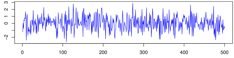
Figure 1: Top: a realization of the observed time series under the null hypothesis (white noise). Bottom: a realization under the alternative with anomalous interval $S=\{201,\dots,250\}$, assuming an ${\rm AR}_{1}$ covariance model with parameter $\psi=0.9$.

Gaussian autoregressive processes and other correlation models are special cases of Gaussian Markov random fields, and therefore this setting is a special case of our general framework, with $\mathcal{C}$ being the class of discrete intervals of length $k$. In the simplest case, the length of the anomalous interval is known beforehand. In more complex settings, it is unknown, in which case $\mathcal{C}$ may be taken to be the class of all intervals within $\mathcal{V}$ of length at least $k_{\rm min}$.

This testing problem has been extensively studied in the slightly different context of change-point analysis, where under the null hypothesis $X_{1},\dots,X_{n}$ are generated from an ${\rm AR}_{h}(\psi^{0})$ process for some $\psi^{0}\in\mathbb{R}^{h}$, while under the alternative hypothesis there is an $i\in\mathcal{V}$ such that $X_{1},\dots,X_{i}$ and $X_{i+1},\dots,X_{n}$ are generated from ${\rm AR}_{h}(\psi^{0})$ and ${\rm AR}_{h}(\psi^{1})$, with $\psi^{0}\neq\psi^{1}$, respectively. The order $h$ is often given. In fact, instead of assuming autoregressive models, nonparametric models are often favored. See, for example, Priestley and Subba Rao (1969); Davis et al. (1995); Giraitis and Leipus (1992); Lavielle and Ludeña (2000); Paparoditis (2009); Hušková et al. (2007); Picard (1985); Horváth (1993) and many other references therein. These papers often suggest maximum likelihood tests whose limiting distributions are studied under the null and (sometimes fixed) alternative hypotheses. For example, in the special case of $h=1$, such a test would reject $\mathcal{H}_{0}$ when $|\hat{\psi}|$ is large, where $\hat{\psi}$ is the maximum likelihood estimate for $\psi$. In particular, from Picard (1985), we can speculate that such a test can asymptotically separate the hypotheses in the simplest setting described above when $\psi k^{\alpha}\to\infty$ for some $\alpha<1/2$ fixed. See also Hušková et al. (2007); Paparoditis (2009) for power analyses against fixed alternatives.

Our general results imply the following in the special case when the anomaly comes in the form of an autoregressive process with unknown parameter $\psi\in\mathbb{R}^{h}$. We note that the order of the autoregressive model $h$ is allowed to grow with $n$ in this asymptotic result.

Corollary 1.

Assume $n,k\to\infty$, and that $h=o\big{(}\sqrt{k/\log(n)}\wedge k^{1/4}\big{)}$. Denote by $\mathfrak{F}(h,r)$ the class of covariance operators corresponding to $AR_{h}$ processes with valid parameter $\psi=(\psi_{1},\ldots,\psi_{h})$ satisfying $\|\psi\|_{2}^{2}\geq r^{2}$. Then $R_{\mathcal{C},\mathfrak{F}(h,r)}^{*}\to 1$ when

$$r^{2}\leq C_{1}\big{(}\log(n/k)/k+\sqrt{h\log(n/k)}/k\big{)}\ .$$ (7)

Conversely, if $f$ denotes the pseudo-likelihood test of Section 4.2, then $R_{\mathcal{C},\mathfrak{F}(h,r)}(f)\to 0$ when

$$r^{2}\geq C_{2}\big{(}\log(n)/k+\sqrt{h\log(n)}/k\big{)}\ .$$ (8)

In both cases, $C_{1}$ and $C_{2}$ denote numerical constants.

Remark 1.

In the interesting setting where $k=n^{\kappa}$ for some $\kappa>0$ fixed, the lower and upper bounds provided by Corollary 1 match up to a multiplicative constant that depends only on $\kappa$.

Despite an extensive literature on the topic, we are not aware of any other minimax optimality result for time series detection.

1.4 Example: detecting a textured region

In image processing, the detection of textured objects against a textured background is relevant in a number of applications, such as in the detection of local fabric defects in the textile industry by automated visual inspection (Kumar, 2008), the detection of a moving object in a textured background (Yilmaz et al., 2006; Kim et al., 2005), the identification of tumors in medical imaging (Karkanis et al., 2003; James et al., 2001), the detection of man-made objects in natural scenery (Kumar and Hebert, 2003), the detection of sites of interest in archeology (Litton and Buck, 1995) and of weeds in crops (Dryden et al., 2003). In all these applications, the object is generally small compared to the size of the image.

Common models for texture include Markov random fields (Cross and Jain, 1983) and joint distributions over filter banks such as wavelet pyramids (Manjunath and Ma, 1996; Portilla and Simoncelli, 2000). We focus here on textures that are generated via Gaussian Markov random fields (Chellappa and Chatterjee, 1985; Zhu et al., 1998). Our goal is to detect a textured object hidden in white noise. For this discussion, we place ourselves in the lattice setting (1) in dimension $d=2$. Just like before, under $\mathcal{H}_{0}$, the $(X_{i}:i\in\mathcal{V})$ are independent standard normal random variables. Under $\mathcal{H}_{1}$, when the region $S\subset\mathcal{V}$ is anomalous, the $(X_{i}:i\notin S)$ are still i.i.d. standard normal, while $(X_{i}:i\in S)\sim(Y_{i}:i\in S)$, where $(Y_{i}:i\in\mathbb{Z}^{2})$ is such that for each $i\in\mathbb{Z}^{2}$, the conditional distribution of $Y_{i}$ given the rest of the variables $Y^{(-i)}:=(Y_{j}:j\neq i)$ is normal with mean

$$\sum_{(t_{1},t_{2})\in[-h,h]^{2}\setminus\{(0,0)\}}\phi_{t_{1},t_{2}}Y_{i+(t_{1},t_{2})}$$ (9)

and variance $\sigma_{\phi}^{2}$, where the $\phi_{t_{1},t_{2}}$’s are the coefficients of the process and $\sigma_{\phi}$ is such that $\operatorname{Var}(Y_{i})=1$ for all $i$. The set of valid parameters $\phi$ is defined in Section 2.1. A simple sufficient condition is $\|\phi\|_{1}=\sum_{(t_{1},t_{2})\in[-h,h]^{2}\setminus\{(0,0)\}}|\phi_{t_{1},t_{2}}|<1$. In this model, the dependency neighborhood of $i\in\mathbb{Z}^{2}$ is $i+[-h,h]^{2}\cap\mathbb{Z}^{2}$. One of the simplest cases is when $h=1$ and $\phi_{t_{1},t_{2}}=\phi$ when $(t_{1},t_{2})\in\{(\pm 1,0),(0,\pm 1)\}$ for some $\phi\in(-1/4,1/4)$, and the anomalous region is a discrete square; see Figure 2 for a realization of the resulting process.

This is a special case of our setting. While intervals are natural in the case of time series, squares are rather restrictive models of anomalous regions in images. We consider instead the “blob-like” regions (to be defined later) that include convex and star-shaped regions.

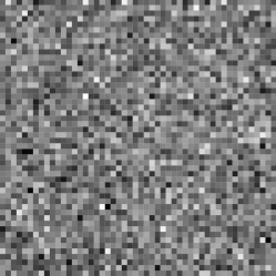
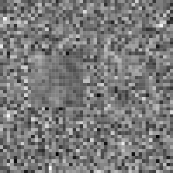
Figure 2: Left: white noise, no anomalous region is present. Right: a squared anomalous region is present. In this example on the $50\times 50$ grid, the anomalous region is a $15\times 15$ square piece from a Gaussian Markov random field with neighborhood radius $h=1$ and coefficient vector $\phi_{t_{1},t_{2}}=\phi:=\frac{1}{4}(1-10^{-4})$ when $(t_{1},t_{2})\in\{(\pm 1,0),(0,\pm 1)\}$, and zero otherwise.

A number of publications address the related problems of texture classification (Kervrann and Heitz, 1995; Zhu et al., 1998; Varma and Zisserman, 2005) and texture segmentation (Jain and Farrokhnia, 1991; Hofmann et al., 1998; Grigorescu et al., 2002; Galun et al., 2003; Malik et al., 2001). In fact, this literature is quite extensive. Only very few papers address the corresponding change-point problem (Shahrokni et al., 2004; Palenichka et al., 2000) and we do not know of any theoretical results in this literature. Our general results (in particular, Corollary 4) imply the following.

Corollary 2.

Assume $n,k\to\infty$, and that $h=o\big{(}\sqrt{k/\log(n)}\wedge k^{1/5}\big{)}$. Denote by $\mathfrak{G}(h,r)$ the class of covariance operators corresponding to stationary Gaussian Markov Random Fields with valid parameter (see Section 2.1 for more details) $\phi=(\phi_{i,j})_{(i,j)\in\{-h,\ldots,h\}^{2}\setminus\{0\}}$ satisfying $\|\phi\|_{2}^{2}\geq r^{2}$. Then $R_{\mathcal{C},\mathfrak{G}(h,r)}^{*}\to 1$ when

$$r^{2}\leq C_{1}\left[\frac{\log(n/k)}{k}+\frac{\sqrt{h^{2}\log(n/k)}}{k}\right]\ .$$ (10)

Conversely, if $f$ denotes the pseudo-likelihood test of Section 4.2, then $R_{\mathcal{C},\mathfrak{G}(h,r)}(f)\to 0$ when

$$r^{2}\geq C_{2}\left[\frac{\log(n/k)}{k}+\frac{\sqrt{h^{2}\log(n/k)}}{k}\right]\ .$$ (11)

In both cases, $C_{1}$ and $C_{2}$ denote positive numerical constants.

Informally, the lower bound on the magnitude of the coefficient vector $\phi$, namely $r^{2}$, quantifies the extent to which the variables $Y_{i}$ are explained by the rest of variables $Y^{(-i)}$ as in (9).

Although not in the literature on change-point or object detection, Anandkumar et al. (2009) is the only other paper developing theory in a similar context. It considers a spatial model where points $\{x_{i},i\in[N]\}$ are sampled uniformly at random in some bounded region and a nearest-neighbor graph is formed. On the resulting graph, variables are observed at the nodes. Under the (simple) null hypothesis, the variables are i.i.d. zero mean normal. Under the (simple) alternative, the variables arise from a Gaussian Markov random with covariance operator of the form $\Gamma_{i,j}\propto g(\|x_{i}-x_{j}\|)$, where $g$ is a known function. The paper analyzes the large-sample behavior of the likelihood ratio test.

1.5 More related work

As we mentioned earlier, the detection-of-means setting is much more prevalent in the literature. When the anomaly has no a priori structure, the problem is that of multiple testing; see, for example, Ingster (1999); Baraud (2002); Donoho and Jin (2004) for papers testing the global null hypothesis. Much closer to what interests us here, the problem of detecting objects with various geometries or combinatorial properties has been extensively analyzed, for example, in some of our earlier work (Arias-Castro et al., 2008; Addario-Berry et al., 2010; Arias-Castro et al., 2011) and elsewhere (Walther, 2010; Desolneux et al., 2003). We only cite a few publications that focus on theory. The applied literature is vast; see Arias-Castro et al. (2011) for some pointers.

Despite its importance in practice, as illustrated by the examples and references given in Sections 1.3 and 1.4, the detection-of-correlations setting has received comparatively much less attention, at least from theoreticians. Here we find some of our own work (Arias-Castro et al., 2012, 2015). In the first of these papers, we consider a sequence $X_{1},\dots,X_{n}$ of standard normal random variables. Under the null, they are independent. Under the alternative, there is a set $S$ in a class of interest $\mathcal{C}$ where the variables are correlated. We consider the unstructured case where $\mathcal{C}$ is the class of all sets of size $k$ (given) and also various structured cases, and in particular, that of intervals. This would appear to be the same as in the present lattice setting in dimension $d=1$, but the important difference is that that correlation operator ${\boldsymbol{\Gamma}}$ is not constrained, and in particular no Markov random field structure is assumed. The second paper extends the setting to higher dimensions, thus testing whether some coordinates of a high-dimensional Gaussian vector are correlated or not. When the correlation structure in the anomaly is arbitrary, the setting overlaps with that of sparse principal component analysis (Berthet and Rigollet, 2013; Cai et al., 2013). The problem is also connected to covariance testing in high-dimensions; see, e.g., Cai and Ma (2013). We refer the reader to the above-mentioned papers for further references.

1.6 Contribution and content

The present paper thus extends previous work on the detection-of-means setting to the detection-of-correlations setting in the (structured) context of detecting signals/objects in time series/images. The paper also extends some of our own work on the detection-of-correlations to Markov random field models, which are typically much more appropriate in the context of detection in signals and images. The theory in the detection-of-correlations setting is more complicated than in the the detection-of-means setting, and in particular deriving exact minimax (first-order) results remains an open problem. Compared to our previous work on the detection-of-correlations setting, the Markovian assumption makes the problem significantly more complex as it requires handling Markov random fields which are conceptually more complex objects. As a result, the proof technique is by-and-large novel, at least in the detection literature.

The rest of the paper is organized as follows. In Section 2 we lay down some foundations on Gaussian Markov Random Fields, and in particular, their covariance operators, and we also derive a general minimax lower bound that is used several times in the paper. In the remainder of the paper, we consider detecting correlations in a finite-dimensional lattice (1), which includes the important special cases of time series and textures in images. We establish lower bounds, both when the covariance matrix is known (Section 3) or unknown (Section 4) and propose test procedures that are shown to achieve the lower bounds up to multiplicative constants. In Section 5, we specialize our general results to specific classes of anomalous regions such as classes of cubes, and more generally, “blobs.” In Section 6 we outline possible generalizations and further work. The proofs are gathered in Section 7.

2 Preliminaries

In this paper we derive upper and lower bounds for the minimax risk, both when ${\boldsymbol{\Gamma}}$ is known as in (3) and when it is unknown as in (5), the latter requiring a substantial amount of additional work. For the sake of exposition, we sketch here the general strategy for obtaining minimax lower bounds by adapting the general strategy initiated in Ingster (1993) to detection-of-correlation problems. This allows us to separate the technique used to derive minimax lower bounds from the technique required to handle Gaussian Markov random fields.

2.1 Some background on Gaussian Markov random fields

We elaborate on the setting described in Sections 1.1 and 1.2. As the process $Y$ is indexed by $\mathbb{Z}^{d}$, note that all the indices $i$ of $\phi$ and ${\boldsymbol{\Gamma}}$ are $d$-dimensional. Given a positive integer $h$, denote by $\mathbb{N}_{h}$ the integer lattice $\{-h,\dots,h\}^{d}\setminus\{0\}^{d}$ with $(2h+1)^{d}-1$ nodes. For any nonsingular covariance operator ${\boldsymbol{\Gamma}}$ of a stationary Gaussian Markov random field over $\mathbb{Z}^{d}$ with unit variance and neighborhood $\mathbb{N}_{h}$, there exists a unique vector $\phi$ indexed by the nodes of $\mathbb{N}_{h}$ satisfying $\phi_{i}=\phi_{-i}$ such that, for all $i,j\in\mathbb{Z}^{d}$,

$${\boldsymbol{\Gamma}}^{-1}_{i,j}/{\boldsymbol{\Gamma}}^{-1}_{i,i}=\begin{cases}-\phi_{i-j}&\text{ if }1\leq|i-j|_{\infty}\leq h,\\ 1&\text{ if }i=j,\\ 0&\text{otherwise~{},}\end{cases}$$ (12)

where ${\boldsymbol{\Gamma}}^{-1}$ denotes the inverse of the covariance operator ${\boldsymbol{\Gamma}}$. Consequently, there exists a bijective map from the collection of invertible covariance operators of stationary Gaussian Markov random fields over $\mathbb{Z}^{d}$ with unit variance and neighborhood $\mathbb{N}_{h}$ to some subset $\Phi_{h}\subset\mathbb{R}^{\mathbb{N}_{h}}$. Given $\phi\in\Phi_{h}$, ${\boldsymbol{\Gamma}}(\phi)$ denotes the unique covariance operator satisfying ${\boldsymbol{\Gamma}}_{i,i}=1$ and (12). It is well known that $\Phi_{h}$ contains the set of vectors $\phi$ whose $\ell_{1}$-norm is smaller than one, that is,

$$\{\phi\in\mathbb{R}^{\mathbb{N}_{h}}:\|\phi\|_{1}<1\}\subset\Phi_{h}\ ,$$

as the corresponding operator ${\boldsymbol{\Gamma}}^{-1}(\phi)$ is diagonally dominant in that case. In fact, the parameter space $\Phi_{h}$ is characterized by the Fast Fourier Transform (FFT) as follows

$$\Phi_{h}=\Big{\{}\phi:\quad 1+\sum_{1\leq|i|_{\infty}\leq h}\phi_{i}\cos(\langle i,\omega\rangle)>0,\quad\forall\omega\in(-\pi,\pi]^{d}\Big{\}}\ ,$$

where and $i\in\mathbb{Z}^{d}$ and $\langle\cdot,\cdot\rangle$ denotes the scalar product in $\mathbb{R}^{d}$. The interested reader is referred to (Guyon, 1995, Sect.1.3) or (Rue and Held, 2005, Sect.2.6) for further details and discussions. For $\phi\in\Phi_{h}$, define $\sigma^{2}_{\phi}=1/{\boldsymbol{\Gamma}}_{i,i}^{-1}(\phi)$.

The correlated process $Y=(Y_{i}:i\in\mathbb{Z}^{d})$ is centered Gaussian with covariance operator ${\boldsymbol{\Gamma}}(\phi)$ is such that, for each $i\in\mathbb{Z}^{d}$, the conditional distribution of $Y_{i}$ given the rest of the variables $Y^{(-i)}$ is

$$Y_{i}|Y^{(-i)}\ \sim\ \mathcal{N}\Big{(}\sum_{j\in\mathbb{N}_{h}}\phi_{j}Y_{i+j},\sigma^{2}_{\phi}\Big{)}\ .$$ (13)

Define the $h$-boundary of $S$, denoted $\Delta_{h}(S)$, as the collection of vertices in $S$ whose distance to $\mathbb{Z}^{d}\setminus S$ is at most $h$. We also define the $h$-interior $S$ as $S^{h}=S\setminus\Delta_{h}(S)$. If $S\subset\mathcal{V}$ is a finite set, we denote by ${\boldsymbol{\Gamma}}_{S}$ the principal submatrix of the covariance operator ${\boldsymbol{\Gamma}}$ indexed by $S$. If ${\boldsymbol{\Gamma}}$ is nonsingular, each such submatrix is invertible.

2.2 A general minimax lower bound

As is standard, an upper bound is obtained by exhibiting a test $f$ and then upper-bounding its risk—either (2) or (4) according to whether ${\boldsymbol{\Gamma}}$ is known or unknown. In order to derive a lower bound for the minimax risk, we follow the standard argument of choosing a prior distribution on the class of alternatives and then lower-bounding the minimax risk with the resulting average risk. When ${\boldsymbol{\Gamma}}$ is known, this leads us to select a prior on $\mathcal{C}$, denoted by $\nu$, and consider

$$\bar{R}_{\nu,{\boldsymbol{\Gamma}}}(f)=\mathbb{P}_{0}\{f(X)=1\}+\sum_{S\in\mathcal{C}}\nu(S)\mathbb{P}_{S,{\boldsymbol{\Gamma}}}\{f(X)=0\}\quad\text{and}\quad\bar{R}^{*}_{\nu,{\boldsymbol{\Gamma}}}=\inf_{f}\bar{R}_{\nu,{\boldsymbol{\Gamma}}}(f)~{}.$$ (14)

The latter is the Bayes risk associated with $\nu$. By placing a prior on the class of alternative distributions, the alternative hypothesis becomes effectively simple (as opposed to composite). The advantage of this is that the optimal test may be determined explicitly. Indeed, the Neyman-Pearson fundamental lemma implies that the likelihood ratio test $f_{\nu,{\boldsymbol{\Gamma}}}^{*}(x)=\mathbb{I}\{L_{\nu,{\boldsymbol{\Gamma}}}(x)>1\}$, with

$$L_{\nu,{\boldsymbol{\Gamma}}}=\sum_{S\in\mathcal{C}}\nu(S)\frac{{\rm d}\mathbb{P}_{S,{\boldsymbol{\Gamma}}}}{{\rm d}\mathbb{P}_{0}}~{},$$

minimizes the average risk. In most of the paper, $\nu$ will be chosen as the uniform distribution on the class $\mathcal{C}$. In this because the sets in $\mathcal{C}$ play almost the same role (although not exactly because of boundary effects).

When ${\boldsymbol{\Gamma}}$ is only known to belong to some class $\mathfrak{G}$ we also need to choose a prior on $\mathfrak{G}$, which we denote by $\pi$, leading to

$$\bar{R}_{\nu,\pi}(f)=\mathbb{P}_{0}\{f(X)=1\}+\sum_{S\in\mathcal{C}}\nu(S)\int\mathbb{P}_{S,{\boldsymbol{\Gamma}}}\{f(X)=0\}\pi({\rm d}{\boldsymbol{\Gamma}})\quad\text{and}\quad\bar{R}^{*}_{\nu,\pi}=\inf_{f}\bar{R}_{\nu,\pi}(f)~{}.$$ (15)

In this case, the likelihood ratio test becomes $f_{\nu,\pi}^{*}(x)=\mathbb{I}\{L_{\nu,\pi}(x)>1\}$, where

$$L_{\nu,\pi}=\sum_{S\in\mathcal{C}}\nu(S)\frac{{\rm d}\mathbb{P}_{S,\pi}}{{\rm d}\mathbb{P}_{0}}~{},\quad\mathbb{P}_{S,\pi}=\int\mathbb{P}_{S,{\boldsymbol{\Gamma}}}\pi({\rm d}{\boldsymbol{\Gamma}})~{},$$

minimizes the average risk.

In both cases, we then proceed to bound the second moment of the resulting likelihood ratio under the null. Indeed, in a general setting, if $L$ is the likelihood ratio for $\operatorname{\mathbb{P}}_{0}$ versus $\operatorname{\mathbb{P}}_{1}$ and $R$ denotes its risk, then (Lehmann and Romano, 2005, Problem 3.10)

$$R=1-\frac{1}{2}\operatorname{\mathbb{E}}_{0}|L(X)-1|\geq 1-\frac{1}{2}\sqrt{\operatorname{\mathbb{E}}_{0}[L(X)^{2}]-1}\ ,$$ (16)

where the inequality follows by the Cauchy-Schwarz inequality.

Remark 2.

Working with the minimax risk (as we do here) allows us to bypass making an explicit choice of prior, although one such choice is eventually made when deriving a lower bound. Another advantage is that the minimax risk is monotone with respect to the class $\mathcal{C}$ in the sense that if $\mathcal{C}^{\prime}\subset\mathcal{C}$, then the minimax risk corresponding to $\mathcal{C}^{\prime}$ is at most as large as that corresponding to $\mathcal{C}$. This monotonicity does not necessarily hold for the Bayes risk. See Addario-Berry et al. (2010) for a discussion in the context of the detection-of-means problem.

We now state a general minimax lower bound. (Recall that all the proofs are in Section 7.) Although the result is stated for a class $\mathcal{C}$ of disjoint subsets, using the monotonicity of the minimax risk, the result can be used to derive lower bounds in more general settings. It is particularly useful in the context of detecting blob-like anomalous regions in the lattice. (The same general approach is also fruitful in the detection-of-means setting.) We emphasize that this result is quite straightforward given the work flow outlined above. The technical difficulties will come with its application to the context that interest us here, which will necessitate a good control of (17) below.

Recall the definition (15).

Proposition 1.

Let $\{{\boldsymbol{\Gamma}}(\phi):\phi\in\Phi\}$ be a class of nonsingular covariance operators and let $\mathcal{C}$ be a class of disjoint subsets of $\mathcal{V}$. Put the uniform prior $\nu$ on $\mathcal{C}$ and let $\pi$ be a prior on $\Phi$. Then

$$\bar{R}^{*}_{\nu,\pi}\geq 1-\frac{1}{2|\mathcal{C}|}\Big{(}\sum_{S\in\mathcal{C}}V_{S}\Big{)}^{1/2}\ ,$$

where

$$V_{S}:=\mathbb{E}_{\pi}\left[\left(\frac{\det({\boldsymbol{\Gamma}}_{S}^{-1}(\phi_{1}))\det({\boldsymbol{\Gamma}}_{S}^{-1}(\phi_{2}))}{\det({\boldsymbol{\Gamma}}_{S}^{-1}(\phi_{1})+{\boldsymbol{\Gamma}}_{S}^{-1}(\phi_{2})-\mathbf{I}_{S})}\right)^{1/2}\right]\ ,$$ (17)

and the expected value is with respect to $\phi_{1},\phi_{2}$ drawn i.i.d. from the distribution $\pi$.

3 Known covariance

We start with the case where the covariance operator ${\boldsymbol{\Gamma}}$ is known. Although this setting is of less practical importance, as this operator is rarely known in applications, we treat this case first for pedagogical reasons and also to contrast with the much more complex setting where the operator is unknown, treated later on.

3.1 Lower bound

Recall the definition of the minimax risk (3) and the average risk (14). (Henceforth, to lighten the notation, we replace subscripts in ${\boldsymbol{\Gamma}}(\phi)$ with subscripts in $\phi$.) For any prior $\nu$ on $\mathcal{C}$, the minimax risk is at least as large as the $\nu$-average risk, $R^{*}_{\mathcal{C},\phi}\geq\bar{R}^{*}_{\nu,\phi}$, and the following corollary of Proposition 1 provides a lower bound on the latter.

Corollary 3.

Let $\mathcal{C}$ be a class of disjoint subsets of $\mathcal{V}$ and fix $\phi\in\Phi_{h}$ satisfying $\|\phi\|_{1}<1/2$. Then, letting $\nu$ denote the uniform prior over $\mathcal{C}$, we have

$$\bar{R}^{*}_{\nu,\phi}\geq 1-\frac{1}{2|\mathcal{C}|}\left[\sum_{S\in\mathcal{C}}\exp\left(\frac{10|S|\|\phi\|_{2}^{2}}{1-2\|\phi\|_{1}}\right)\right]^{1/2}\ .$$ (18)

In particular, the corollary implies that, for any fixed $a\in(0,1)$, $R^{*}_{\mathcal{C},\phi}\geq 1-a$ as soon as

$$\frac{\|\phi\|_{2}^{2}}{1-2\|\phi\|_{1}}\leq\min_{S\in\mathcal{C}}\frac{\log\left(4|\mathcal{C}|/a^{2}\right)}{10|S|}~{}.$$ (19)

Furthermore, the hypotheses merge asymptotically (i.e., $R^{*}_{\mathcal{C},\phi}\to 1$) when

$$\log(|\mathcal{C}|)-\frac{10\|\phi\|_{2}^{2}}{1-2\|\phi\|_{1}}\max_{S\in\mathcal{C}}|S|\to\infty~{}.$$ (20)

Remark 3.

The condition $\|\phi\|_{1}<1/2$ in Corollary 3 is technical and likely an artifice of our proof method. This condition arises from the term $\det^{-1/2}(2{\boldsymbol{\Gamma}}_{S}(\phi)-\mathbf{I}_{S})$ in $V_{S}$ in (17). For this determinant to be positive, the smallest eigenvalue of ${\boldsymbol{\Gamma}}_{S}(\phi)$ has to be larger than $1/2$, which in turn is enforced by $\|\phi\|_{1}<1/2$. In order to remove, or at least improve on this constraint, we would need to adopt a more subtle approach than applying the Cauchy-Schwarz inequality in (16). We did not pursue this as typically one is interested in situations where $\phi$ is small — see, for example, how the result is applied in Section 5.

3.2 Upper bound: the generalized likelihood ratio test

When the covariance operator ${\boldsymbol{\Gamma}}(\phi)$ is known, the generalized likelihood ratio test rejects the null hypothesis for large values of

$$\max_{S\in\mathcal{C}}\ X_{S}^{\top}(\mathbf{I}_{S}-{\boldsymbol{\Gamma}}_{S}^{-1}(\phi))X_{S}~{}.$$

We use instead the statistic

$$U(X)=\max_{S\in\mathcal{C}}\ \frac{X_{S}^{\top}(\mathbf{I}_{S}-{\boldsymbol{\Gamma}}_{S}^{-1}(\phi))X_{S}-\operatorname{Tr}(\mathbf{I}_{S}-{\boldsymbol{\Gamma}}_{S}^{-1}(\phi))}{\|\mathbf{I}_{S}-{\boldsymbol{\Gamma}}_{S}^{-1}(\phi)\|_{F}\sqrt{\log(|\mathcal{C}|)}+\|\mathbf{I}_{S}-{\boldsymbol{\Gamma}}_{S}^{-1}(\phi)\|\log(|\mathcal{C}|)}~{},$$ (21)

which is based on the centering and normalization the statistics $X_{S}^{\top}(\mathbf{I}_{S}-{\boldsymbol{\Gamma}}_{S}^{-1}(\phi))X_{S}$ where $S\in\mathcal{C}$.

In the following result, we implicitly assume that $|\mathcal{C}|\to\infty$, which is the most interesting case.

Proposition 2.

Assume that $\phi\in\Phi_{h}$ satisfies $\|\phi\|_{1}\leq\eta<1$ and that $|S^{h}|\geq|S|/2$. The test $f(x)=\mathbb{I}\{U(x)>4\}$ has risk $R_{\mathcal{C},\phi}(f)\leq 2/|\mathcal{C}|$ when

$$\|\phi\|_{2}^{2}\min_{S\in\mathcal{C}}|S|\geq C_{0}\log(|\mathcal{C}|)\ ,$$ (22)

where $C_{0}>0$ only depends on the dimension $d$ of the lattice and $\eta$.

Comparing with Condition (20), we see that condition (22) matches (up to constants) the minimax lower bound, so that (at least when $\|\phi\|_{1}<1/2$) the normalized generalized likelihood ratio test based on (21) is asymptotically minimax up to a multiplicative constant. The $\ell_{1}$-norm $\|\phi\|_{1}$ arises in the proof of Corollary 3 when bounding the largest eigenvalue of ${\boldsymbol{\Gamma}}(\phi)$ (see Lemma 5).

4 Unknown covariance

We now consider the case where the covariance operator ${\boldsymbol{\Gamma}}(\phi)$ of the anomalous Gaussian Markov random field is unknown. We therefore start by defining a class of covariance operators via a class of vectors $\phi$. Given a positive integer $h>0$ and some $r>0$, define

$$\Phi_{h}(r):=\{\phi\in\Phi_{h},\ \|\phi\|_{2}\geq r\}\ ,$$ (23)

and let

$$\mathfrak{G}(h,r):=\{{\boldsymbol{\Gamma}}(\phi):\phi\in\Phi_{h}(r)\}~{},$$ (24)

which is the class of covariance operators corresponding to stationary Gaussian Markov Random Fields with parameter in the class (23).

4.1 Lower bound

The theorem below establishes a lower bound for the risk following the approach outlined in Section 2, which is based on the choice of a suitable prior $\pi$ on $\Phi_{h}$, defined as follows. By symmetry of the elements of $\Phi_{h}$, one can fix a sublattice $\mathbb{N}^{\prime}_{h}$ of size $|\mathbb{N}_{h}|/2$ such that any $\phi\in\Phi_{h}$ is uniquely defined (via symmetry) by its restriction to $\mathbb{N}^{\prime}_{h}$. Choose the distribution $\pi$ such that $\phi\sim\pi$ is the unique extension to $\mathbb{N}_{h}$ of the random vector $r|\mathbb{N}_{h}|^{-1/2}\xi$, where the coordinates of the random vector $\xi$—indexed by $\mathbb{N}^{\prime}_{h}$—are i.i.d. Rademacher random variables (i.e., symmetric $\pm 1$-valued random variables). Note that, if $r|\mathbb{N}_{h}|<1$, $\pi$ is acceptable since it concentrates on the set $\{\phi\in\Phi_{h},\ \|\phi\|_{2}=r\}\subset\Phi_{h}(r)$. Recall the definition of the minimax risk (5) and the average risk (15). As before, for any priors $\nu$ on $\mathcal{C}$ and $\pi$ on $\Phi_{h}(r)$, the minimax risk is at least as large as the average risk with these priors, $R^{*}_{\mathcal{C},\mathfrak{G}(h,r)}\geq\bar{R}^{*}_{\nu,\pi}$, and the following (much more elaborate) corollary of Proposition 1 provides a lower bound on the latter.

Theorem 1.

There exists a constant $C_{0}>0$ such that the following holds. Let $\mathcal{C}$ be a class of disjoint subsets of $\mathcal{V}$ and let $\nu$ denote the uniform prior over $\mathcal{C}$. Let $a\in(0,1)$ and assume that the neighborhood size $|\mathbb{N}_{h}|$ satisfies

$$|\mathbb{N}_{h}|\leq\min_{S\in\mathcal{C}}\left[\frac{|S|}{\log\left(|\mathcal{C}|/a\right)}\bigwedge|S|^{2/5}\log^{1/5}\left(|\mathcal{C}|/a\right)\bigwedge\left(\frac{|S|}{|\Delta_{2h}(S)|}\right)^{2}\log^{-1/6}\left(|\mathcal{C}|/a\right)\right]\ .$$ (25)

Then $\bar{R}^{*}_{\nu,\pi}\geq 1-a$ as soon as

$$r^{2}\max_{S\in\mathcal{C}}|S|\leq C_{0}\left[\sqrt{|\mathbb{N}_{h}|\log\left(|\mathcal{C}|/a\right)}\bigvee\log\left(|\mathcal{C}|/a\right)\right]\ .$$ (26)

This bound is our main impossibility result. Its proof relies on a number auxiliary results for Gaussian Markov Random Fields (Section 7.3) that may useful for other problems of estimating Gaussian Markov Random Fields. Notice that the second term in (26) is what appears in (19), which we saw arises in the case where the covariance is known. In light of this fact, we may interpret the first term in (26) as the ‘price to pay’ for adapting to an unknown covariance operator in the class of covariance operators of Gaussian Markov random fields with dependency radius $h$.

4.2 Upper bound: a Fisher-type test

We introduce a test whose performance essentially matches the minimax lower bound of Theorem 1. Comparatively, the construction and analysis of this test is much more involved than that of the generalized likelihood ratio test of Section 3.2.

Let $F_{i}=(X_{i+v}:1\leq|v|_{\infty}\leq h)$, seen as a vector, and let $\mathbf{F}_{S,h}$ be the matrix with row vectors $F_{i},i\in S^{h}$. Also, let $X_{S,h}=(X_{i}:i\in S^{h})$. Under the null hypothesis, each variable $X_{i}$ is independent of $F_{i}$, although $X_{i}$ is correlated with some $(F_{j},j\neq i)$. Under the alternative hypothesis, there exists a subset $S$ and a vector $\phi\in\Phi_{h}$ such that

$$X_{S,h}=\mathbf{F}_{S,h}\phi+\epsilon_{S,h}\ ,$$ (27)

where each component $\epsilon_{i}$ of $\epsilon_{S,h}$ is independent of the corresponding vector $F_{i}$, but the $\epsilon_{i}$’s are not necessarily independent. Equation (27) is the so-called conditional autoregressive (CAR) representation of a Gaussian Markov random field (Guyon, 1995). For Gaussian Markov random fields, the celebrated pseudo-likelihood method (Besag, 1975) amounts to estimating $\phi$ by taking least-squares in (27).

Returning to our testing problem, observe that the null hypothesis is true if and only if all the parameters of the conditional expectation of $X_{S,h}$ given $\mathbf{F}_{S,h}$ are zero. In analogy with the analysis-of-variance approach for testing whether the coefficients of a linear regression model are all zero, we consider a Fisher-type statistic

$$T^{*}=\max_{S\in\mathcal{C}}T_{S}\ ,\quad\quad T_{S}:=\frac{|S^{h}|\|\boldsymbol{\Pi}_{S,h}X_{S,h}\|_{2}^{2}}{\|X_{S,h}-\boldsymbol{\Pi}_{S,h}X_{S,h}\|_{2}^{2}}\ ,$$ (28)

where $\boldsymbol{\Pi}_{S,h}:=\mathbf{F}_{S,h}(\mathbf{F}_{S,h}^{\top}\mathbf{F}_{S,h})^{-1}\mathbf{F}^{\top}_{S,h}$ is the orthogonal projection onto the column space of $\mathbf{F}_{S,h}$. Since in the linear model (27) the response vector $X_{S,h}$ is not independent of the design matrix $\mathbf{F}_{S,h}$, the statistic $T_{S}$ does not follow an $F$-distribution. Nevertheless, we are able to control the deviations of $T^{*}$, both under null and alternative hypotheses, leading to the following performance bound. Recall the definition (4).

Theorem 2.

There exist four positive constants $C_{1},C_{2},C_{3},C_{4}$ depending only on $d$ such that the following holds. Assume that

$$|\mathbb{N}_{h}|^{4}\vee|\mathbb{N}_{h}|^{2}\log(|\mathcal{C}|)\leq C_{1}\min_{S\in\mathcal{C}}|S^{h}|\ .$$ (29)

Fix $\alpha$ and $\beta$ in $(0,1)$ such that

$$\log(\tfrac{1}{\alpha})\vee\log(\tfrac{1}{\beta})\leq C_{2}\frac{\min_{S\in\mathcal{C}}|S^{h}|}{|\mathbb{N}_{h}|^{2}\log(|\mathcal{C}|)}\ .$$ (30)

Then, under the null hypothesis,

$$\operatorname{\mathbb{P}}\left\{T^{*}\geq|\mathbb{N}_{h}|+C_{3}\left[\sqrt{|\mathbb{N}_{h}|(\log(|\mathcal{C}|)+1+\log(\alpha^{-1}))}+\log(|\mathcal{C}|)+\log(\alpha^{-1})\right]\right\}\leq\alpha\ ,$$ (31)

while under the alternative,

$$\operatorname{\mathbb{P}}\left\{T^{*}\geq|\mathbb{N}_{h}|+C_{4}\left[|S^{h}|\left(\|\phi\|_{2}^{2}\wedge\frac{1}{|\mathbb{N}^{h}|}\right)-\sqrt{\mathbb{N}_{h}}(1+\log^{4}(\beta^{-1}))\right]\right\}\geq 1-\beta\ .$$ (32)

In particular, if $\alpha_{n},\beta_{n}\to 0$ are arbitrary positive sequences, then the test $f$ that rejects the null hypothesis if

$$T^{*}\geq|\mathbb{N}_{h}|+C_{3}\left[\sqrt{|\mathbb{N}_{h}|(\log(|\mathcal{C}|)+1+\log(\alpha_{n}^{-1}))}+\log(|\mathcal{C}|)+\log(\alpha_{n}^{-1})\right]$$

satisfies $R_{\mathcal{C},\mathfrak{G}(h,r)}(f)\to 0$ as soon as

$$r^{2}>\frac{C_{0}}{\min_{S\in\mathcal{C}}|S^{h}|}\left[\sqrt{|\mathbb{N}_{h}|\left(\log(|\mathcal{C}|)+\log(\tfrac{1}{\alpha_{n}})+\log^{8}(\tfrac{1}{\beta_{n}})\right)}\bigvee\log(|\mathcal{C}|)\bigvee\log(\tfrac{1}{\alpha_{n}})\right]\ ,$$ (33)

where $C_{0}>0$ depends only on $d$.

Comparing with the minimax lower bound established in Theorem 1, we see that this test is nearly optimal with respect to $h$, the size of the collection $|\mathcal{C}|$, and the size $|S|$ of the anomalous region (under the alternative).

5 Examples: cubes and blobs

In this section we specialize our general results proved in the previous subsections to classes of cubes, and more generally, blobs.

5.1 Cubes

Consider the problem of detecting an anomalous cube-shaped region. Let $\ell\in\{1,\dots,m\}$ and assume that $m$ is an integer multiple of $\ell$ (for simplicity). Let $\mathcal{C}$ denote the class of all discrete hypercubes of side length $\ell$, that is, sets of the form $S=\prod_{s=1}^{d}\{b_{s},\ldots,b_{s}+\ell-1\}$, where $b_{s}\in\{1,\ldots,m+1-\ell\}$. Each such hypercube $S\in\mathcal{C}$ contains $|S|=k:=\ell^{d}$ nodes, and the class is of size $|\mathcal{C}|=(m-1-\ell)^{d}\leq n$.

The lower bounds for the risk established in Corollary 3 and Theorem 1 are not directly applicable here since these results require subsets of the class $\mathcal{C}$ to be disjoint. However, they apply to any subclass $\mathcal{C}^{\prime}\subset\mathcal{C}$ of disjoint subsets and, as mentioned in Section 2, any lower bound on the minimax risk over $\mathcal{C}^{\prime}$ applies to the minimax risk over $\mathcal{C}$. A natural choice for $\mathcal{C}^{\prime}$ here is that of all cubes of the form $S=\prod_{s=1}^{d}\{a_{s}\ell+1,\dots,(a_{s}+1)\ell\}$, where $a_{s}\in\{0,\dots,m/\ell-1\}$. Note that $|\mathcal{C}^{\prime}|=(m/\ell)^{d}=n/k$.

$h$ bounded. Consider first the case where the radius $h$ of the neighborhood is bounded. We may apply Corollary 3 to get

$$R^{*}_{\mathcal{C},\phi}\geq 1-\frac{k^{1/2}}{2n^{1/2}}\exp\left\{\frac{5k\|\phi\|_{2}^{2}}{1-2\|\phi\|_{1}}\right\}\ .$$

For a given $r>0$ satisfying $2|\mathbb{N}_{h}|r\leq 1$, we can choose a parameter $\phi$ constant over $\mathbb{N}_{h}$ such that $\|\phi\|_{2}=r$ and $\|\phi\|_{1}=r\sqrt{(2h+1)^{d}-1}$. Since $R^{*}_{\mathcal{C},\mathfrak{G}(h,r)}\geq R^{*}_{\mathcal{C},\phi}$, we thus have $R^{*}_{\mathcal{C},\mathfrak{G}(h,r)}\to 1$ when $n\to\infty$, if $(k,\phi)=(k(n),\phi(n))$ satisfies $\log(n)\ll k\ll n$ and $r^{2}\leq\log(n/k)/(11k)$. Comparing with the performance of the Fisher test of Section 4.2, in this particular case, Condition (29) is met, and letting $\alpha=\alpha(n)\to 0$ and $\beta=\beta(n)\to 0$ slowly, we conclude from (33) that this test (denoted $f$) has risk $R_{\mathcal{C},\mathfrak{G}(h,r)}(f)\to 0$ when $r^{2}\geq C_{0}\log(n)/k$ for some constant $C_{0}$. Thus, in this setting, the Fisher test, without knowledge of $\phi$, achieves the correct detection rate as long as $k\leq n^{b}$ for some fixed $b<1$.

$h$ unbounded. When $h$ is unbounded, we obtain a sharper bound by using Theorem 1 instead of Corollary 3. Specialized to the current setting, we derive the following.

Corollary 4.

There exist two positive constants $C_{1}$ and $C_{2}$ depending only on $d$ such that the following holds. Assume that the neighborhood size $h$ is small enough that

$$|\mathbb{N}_{h}|\leq C_{1}\left[\frac{k}{\log^{1\vee(d/2)}\left(\frac{n}{k}\right)}\bigwedge k^{2/5}\log^{1/5}\left(\frac{n}{k}\right)\bigwedge d^{-\frac{2d}{d+2}}k^{\frac{2}{d+2}}\log^{\frac{d}{3d+6}}\left(\frac{n}{k}\right)\right]\ .$$ (34)

Then the minimax risk tends to one when $n\to\infty$ as soon as $(k,h,r)=(k(n),h(n),r(n))$ satisfies $n/k\rightarrow\infty$ and

$$r^{2}\leq C_{2}\left[\frac{\log(\tfrac{n}{k})}{k}\bigvee\frac{\sqrt{|\mathbb{N}_{h}|\log(\tfrac{n}{k})}}{k}\right]\ .$$ (35)

Note that, in the case of a square neighborhood, $|\mathbb{N}_{h}|=(2h+1)^{d}-1$. Comparing with the performance of the Fisher test, in this particular case, Condition (29) is equivalent to $|\mathbb{N}_{h}|\leq C_{0}\big{(}k^{1/4}\wedge\sqrt{k/\log(n)}\big{)}$ for some constant $C_{0}$. When $k$ is polynomial in $n$, this condition is stronger than Condition (34) unless $d\leq 5$. In any case, assuming $h$ is small enough that both (29) and (34) hold, and letting $\alpha=\alpha(n)\to 0$ and $\beta=\beta(n)\to 0$ slowly, we conclude from (33) that the Fisher test has risk $R_{\mathcal{C},\mathfrak{G}(h,r)}$ tending to zero when

$$r^{2}\geq C_{0}\left[\frac{\log(n)}{k}\bigvee\frac{\sqrt{|\mathbb{N}_{h}|\log(n)}}{k}\right],$$

for some large-enough constant $C_{0}>0$, matching the lower bound (35) up to a multiplicative constant as long as $k\leq n^{b}$ for some fixed $b<1$.

In conclusion, whether $h$ is fixed or unbounded but growing slowly enough, the Fisher test achieves a risk matching the lower bound up to a multiplicative constant.

5.2 Blobs

So far, we only considered hypercubes, but our results generalize immediately to much larger classes of blob-like regions. Here, we follow the same strategy used in the detection-of-means setting, for example, in Arias-Castro et al. (2005); Arias-Castro et al. (2011); Huo and Ni (2009).

Fix two positive integers $\ell_{\circ}\leq\ell^{\circ}$ and let $\mathcal{C}$ be a class of subsets $S$ such that there are hypercubes $S_{\circ}$ and $S^{\circ}$, of respective side lengths $\ell_{\circ}$ and $\ell^{\circ}$, such that $S_{\circ}\subset S\subset S^{\circ}$. Letting $\mathcal{C}_{\circ}$ and $\mathcal{C}^{\circ}$ denote the classes of hypercubes of side lengths $\ell_{\circ}$ and $\ell^{\circ}$, respectively, our lower bound for the worst-case risk associated with the class $\mathcal{C}^{\circ}$ obtained from Corollary 4 applies directly to $\mathcal{C}$—although not completely obvious, this follows from our analysis—while scanning over $\mathcal{C}_{\circ}$ in the Fisher test yields the performance stated above for the class of cubes. In particular, if $\ell_{\circ}/\ell^{\circ}$ remains bounded away from $0$, the problem of detecting a region in $\mathcal{C}$ is of difficulty comparable to detecting a hypercube in $\mathcal{C}_{\circ}$ or $\mathcal{C}^{\circ}$.

When the size of the anomalous region $k$ is unknown, meaning that the class $\mathcal{C}$ of interest includes regions of different sizes, we can simply scan over dyadic hypercubes as done in the first step of the multiscale method of Arias-Castro et al. (2005). This does not change the rate as there are less than $2n$ dyadic hypercubes. See also Arias-Castro et al. (2011).

We note that when $\ell_{\circ}/\ell^{\circ}=o(1)$, scanning over hypercubes may not be very powerful. For example, for “convex” sets, meaning when

$$\mathcal{C}=\Big{\{}S=K\cap\mathcal{V}:K\subset\mathbb{R}^{d}\text{ convex},|K\cap\mathcal{V}|=k\Big{\}}~{},$$

it is more appropriate to scan over ellipsoids due to John’s ellipsoid theorem (John, 1948), which implies that for each convex set $K\subset\mathbb{R}^{d}$, there is an ellipsoid $E\subset K$ such that ${\rm vol}(E)\geq d^{-d}{\rm vol}(K)$. For the case where $d=2$ and the detection-of-means problem, Huo and Ni (2009)—expanding on ideas proposed in Arias-Castro et al. (2005)—scan over parallelograms, which can be done faster than scanning over ellipses.

Finally, we mention that what we said in this section may apply to other types of regular lattices, and also to lattice-like graphs such as typical realizations of a random geometric graph. See Arias-Castro et al. (2011); Walther (2010) for detailed treatments in the detection-of-means setting.

6 Discussion

We provided lower bounds and proposed near-optimal procedures for testing for the presence of a piece of a Gaussian Markov random field. These results constitute some of the first mathematical results for the problem of detecting a textured object in a noisy image. We leave open some questions and generalization of interest.

More refined results. We leave behind the delicate and interesting problem of finding the exact detection rates, with tight multiplicative constants. This is particularly appealing for simple settings such as finding an interval of an autoregressive process, as described in Section 1.3. Our proof techniques, despite their complexity, are not sufficiently refined to get such sharp bounds. We already know that, in the detection-of-means setting, bounding the variance of the likelihood ratio does not yield the right constant. The variant which consists of bounding the first two moments of a carefully truncated likelihood ratio, possibly pioneered in Ingster (1999), is applicable here, but the calculations are quite complicated and we leave them for future research.

Texture over texture. Throughout the paper we assumed that the background is Gaussian white noise. This is not essential, but makes the narrative and results more accessible. A more general, and also more realistic setting, would be that of detecting a region where the dependency structure is markedly different from the remainder of the image. This setting has been studied in the context of time series, for example, in some of the references given in Section 1.3. However, we are not aware of existing theoretical results in higher-dimensional settings such as in images.

Other dependency structures. We focused on Markov random fields with limited neighborhood range (quantified by $h$ earlier in the paper). This is a natural first step, particularly since these are popular models for time series and textures. However, one could envision studying other dependency structures, such as short-range dependency, defined in Samorodnitsky (2006) as situations where the covariances are summable in the following sense

$$\sup_{i\in\mathcal{V}_{\infty}}\sum_{j\in\mathcal{V}_{\infty}\setminus i}|{\boldsymbol{\Gamma}}_{i,j}|<\infty\ .$$

7 Proofs

7.1 Proof of Proposition 1

The Bayes risk is achieved by the likelihood ratio test $f_{\nu,\pi}^{*}(x)=\mathbb{I}\{L_{\nu,\pi}(x)>1\}$ where

$$L_{\nu,\pi}(x)=\frac{1}{|\mathcal{C}|}\sum_{S\in\mathcal{C}}L_{S}(x)~{},\text{ with}\quad L_{S}(x)=\int\frac{{\rm d}\mathbb{P}_{S,{\boldsymbol{\Gamma}}(\phi)}(x)}{{\rm d}\mathbb{P}_{0}(x)}\pi({\rm d}\phi)~{}.$$

In our Gaussian model,

$$L_{S}(x)=\mathbb{E}_{\pi}\left[\exp\left(\tfrac{1}{2}x_{S}^{\top}(\mathbf{I}_{S}-{\boldsymbol{\Gamma}}_{S}^{-1}(\phi))x_{S}-\tfrac{1}{2}\log\det({\boldsymbol{\Gamma}}_{S}(\phi))\right)\right]~{},$$ (36)

where the expectation is taken with respect to the random draw of $\phi\sim\pi$. Then, by (16),

$$\bar{R}^{*}_{\nu,\pi}=1-\frac{1}{2}\operatorname{\mathbb{E}}_{0}|L_{\nu,\pi}(X)-1|\geq 1-\frac{1}{2}\sqrt{\operatorname{\mathbb{E}}_{0}[L_{\nu,\pi}(X)^{2}]-1}\ .$$ (37)

(Recall that $\mathbb{E}_{0}$ stands for expectation with respect to the standard normal random vector $X$.)

We proceed to bound the second moment of the likelihood ratio under the null hypothesis. Summing over $S,T\in\mathcal{C}$, we have

$$\operatorname{\mathbb{E}}_{0}[L_{\nu,\pi}(X)^{2}]$$

$$= \frac{1}{|\mathcal{C}|^{2}}\sum_{S,T\in\mathcal{C}}\operatorname{\mathbb{E}}_{0}[L_{S}(X)L_{T}(X)]$$

$$= \frac{1}{|\mathcal{C}|^{2}}\sum_{S\neq T}\operatorname{\mathbb{E}}_{0}[L_{S}(X)]\operatorname{\mathbb{E}}_{0}[L_{T}(X)]+\frac{1}{|\mathcal{C}|^{2}}\sum_{S\in\mathcal{C}}\operatorname{\mathbb{E}}_{0}[L_{S}^{2}(X)]$$

$$= \frac{|\mathcal{C}|-1}{|\mathcal{C}|}+\frac{1}{|\mathcal{C}|^{2}}\sum_{S\in\mathcal{C}}\operatorname{\mathbb{E}}_{0}\mathbb{E}_{\pi}\Big{[}\exp\Big{(}X_{S}^{\top}\big{(}\mathbf{I}_{S}-\tfrac{1}{2}{\boldsymbol{\Gamma}}_{S}^{-1}(\phi_{1})-\tfrac{1}{2}{\boldsymbol{\Gamma}}_{S}^{-1}(\phi_{2})\big{)}X_{S}$$

$$\qquad\qquad\qquad\qquad\qquad\qquad-\tfrac{1}{2}\log\det({\boldsymbol{\Gamma}}_{S}(\phi_{1}))-\tfrac{1}{2}\log\det({\boldsymbol{\Gamma}}_{S}(\phi_{2}))\Big{)}\Big{]}$$

$$\leq 1+\frac{1}{|\mathcal{C}|^{2}}\sum_{S}\mathbb{E}_{\pi}\Big{[}\exp\Big{(}-\tfrac{1}{2}\log\det({\boldsymbol{\Gamma}}_{S}^{-1}(\phi_{1})+{\boldsymbol{\Gamma}}_{S}^{-1}(\phi_{2})-\mathbf{I}_{S})-\tfrac{1}{2}\log\det({\boldsymbol{\Gamma}}_{S}(\phi_{1}){\boldsymbol{\Gamma}}_{S}(\phi_{2}))\Big{)}\Big{]}$$

$$= 1+\frac{1}{|\mathcal{C}|^{2}}\sum_{S}V_{S}\ ,$$

where in the second equality we used the fact that $S\neq T$ are disjoint, and therefore $L_{S}(X)$ and $L_{T}(X)$ are independent, and in the third we used the fact that $\operatorname{\mathbb{E}}_{0}[L_{S}(X)]=1$ for all $S\in\mathcal{C}$.

7.2 Deviation inequalities

Here we collect a few more-or-less standard inequalities that we need in the proofs. We start with the following standard tail bounds for Gaussian quadratic forms. See, e.g., Example 2.12 and Exercise 2.9 in Boucheron et al. (2013).

Lemma 1.

Let $Z$ be a standard normal vector in $\mathbb{R}^{d}$ and let $\mathbf{R}$ be a symmetric $d\times d$ matrix. Then

$$\mathbb{P}\left\{Z^{\top}\mathbf{R}Z-\operatorname{Tr}(\mathbf{R})\geq 2\|\mathbf{R}\|_{F}\sqrt{t}+2\|\mathbf{R}\|t\,\right\}\leq e^{-t},\quad\forall t\geq 0~{}.$$

Furthermore, if the matrix $\mathbf{R}$ is positive semidefinite, then

$$\mathbb{P}\left\{Z^{\top}\mathbf{R}Z-\operatorname{Tr}(\mathbf{R})\leq-2\|\mathbf{R}\|_{F}\sqrt{t}\,\right\}\leq e^{-t},\quad\forall t\geq 0.$$

Lemma 2.

There exists a positive constant $C$ such that the following holds. For any Gaussian chaos $Z$ up to order $4$ and any $t>0$,

$$\operatorname{\mathbb{P}}\left\{|Z-\operatorname{\mathbb{E}}[Z]|\geq C\operatorname{Var}^{1/2}(Z)t^{2}\right\}\leq e^{-t}\ .$$

Proof.

This deviation inequality is a consequence of the hypercontractivity of Gaussian chaos. More precisely, Theorem 3.2.10 and Corollary 3.2.6 in de la Peña and Giné (1999) state that

$$\operatorname{\mathbb{E}}\exp\left[\left(\frac{Z-\operatorname{\mathbb{E}}[Z]}{C\operatorname{Var}^{1/2}(Z)}\right)^{1/2}\right]\leq 2\ ,$$

where $C$ is a numerical constant. Then, we apply Markov inequality to prove the lemma. ∎

Lemma 3.

There exists a positive constant $C$ such that the following holds. Let $F$ be a compact set of symmetric $r\times r$ matrices and let $Y\sim\mathcal{N}(0,\mathbf{I}_{r})$. For any $t>0$, the random variable $Z:=\sup_{\mathbf{R}\in F}\operatorname{Tr}\left[\mathbf{R}YY^{\top}\right]$ satisfies

$$\mathbb{P}\{Z\geq\mathbb{E}(Z)+t\}\leq\exp\left(-C\left(\frac{t^{2}}{\mathbb{E}(W)}\bigwedge\frac{t}{B}\right)\right),$$ (38)

where $W:=\sup_{\mathbf{R}\in F}\operatorname{Tr}(\mathbf{R}YY^{\top}\mathbf{R})$ and $B:=\sup_{\mathbf{R}\in F}\|\mathbf{R}\|$.

A slight variation of this result where $Z$ is replaced by $\sup_{\mathbf{R}\in F}\operatorname{Tr}\left[\mathbf{R}(YY^{\top}-\mathbf{I}_{r})\right]$ is proved in Verzelen (2010) using the exponential Efron-Stein inequalities of Boucheron et al. (2005). Their arguments straightforwardly adapt to Lemma 3.

Lemma 4 (Davidson and Szarek (2001)).

Let $\mathbf{W}$ be a standard Wishart matrix with parameters $(n,d)$ satisfying $n>d$. Then for any number $0<x<1$,

$$\mathbb{P}\left\{\lambda^{\rm max}(\mathbf{W})\geq n\left(1+\sqrt{d/n}+\sqrt{2x/n}\right)^{2}\right\} \leq e^{-x}\ ,$$

$$\mathbb{P}\left\{\lambda^{\rm min}(\mathbf{W})\leq n\left(1-\sqrt{d/n}-\sqrt{2x/n}\right)_{+}^{2}\right\} \leq e^{-x}\ .$$

7.3 Auxiliary results for Gaussian Markov random fields on the lattice

He we gather some technical tools and proofs for Gaussian Markov random fields on the lattice. Recall the notation introduced in Section 2.1.

Lemma 5.

For any positive integer $h$ and $\phi\in\Phi_{h}$ with $\|\phi\|_{1}<1$, we have that if $\lambda$ is an eigenvalue of the covariance operator ${\boldsymbol{\Gamma}}(\phi)$, then

$$\frac{\sigma_{\phi}^{2}}{1+\|\phi\|_{1}}\leq\lambda\leq\frac{\sigma_{\phi}^{2}}{1-\|\phi\|_{1}}~{}.$$

Also, we have

$$\frac{\|\phi\|_{2}^{2}}{1+\|\phi\|_{1}}\leq\frac{1-\sigma^{2}_{\phi}}{\sigma^{2}_{\phi}}\leq\frac{\|\phi\|_{2}^{2}}{1-\|\phi\|_{1}}\ \quad\quad\text{ and }\quad\quad 1-\|\phi\|_{1}\leq\sigma_{\phi}^{2}\leq 1~{}.$$ (39)

Proof.

Recall that $\|\cdot\|$ denotes the $\ell^{2}\to\ell^{2}$ operator norm. First note that by the definition of $\phi$, $\sigma_{\phi}^{2}{\boldsymbol{\Gamma}}^{-1}(\phi)-\mathbf{I}=(\phi_{i-j})_{i,j\in\mathbb{Z}^{d}}$, and therefore

$$\|\sigma_{\phi}^{2}{\boldsymbol{\Gamma}}^{-1}(\phi)-\mathbf{I}\|\leq\|\phi\|_{1}~{},$$ (40)

where whe used the bound $\|\mathbf{A}\|\leq\sup_{i\in\mathbb{Z}^{d}}\sum_{j\in\mathbb{Z}^{d}}|\mathbf{A}_{ij}|$. This implies that the largest eigenvalue of ${\boldsymbol{\Gamma}}(\phi)$ is bounded by $\sigma^{2}_{\phi}/(1-\|\phi\|_{1})$ if $\|\phi\|_{1}<1$ and that the smallest eigenvalue of ${\boldsymbol{\Gamma}}(\phi)$ is at least $\sigma^{2}_{\phi}/(1+\|\phi\|_{1})$. Considering the conditional regression of $Y_{i}$ given $Y_{-i}$ mentioned above, that is,

$$Y_{i}=-\sum_{1\leq|j|_{\infty}\leq h}\phi_{j}Y_{i+j}+\epsilon_{i}$$

(with $\epsilon_{i}$ being standard normal independent of the $Y_{j}$ for $j\neq i$) and taking the variance of both sides, we obtain

$$1-\sigma^{2}_{\phi}=\operatorname{Var}\left[\sum_{1<|j|_{\infty}\leq h}\phi_{j}Y_{i+j}\right]=\phi^{\top}{\boldsymbol{\Gamma}}(\phi)\phi\leq\|{\boldsymbol{\Gamma}}(\phi)\|\|\phi\|_{2}^{2}\leq\frac{\|\phi\|_{2}^{2}}{1-\|\phi\|_{1}}\sigma^{2}_{\phi}~{},$$

and therefore

$$1-\sigma^{2}_{\phi}\leq\frac{\|\phi\|_{2}^{2}}{1-\|\phi\|_{1}}\sigma^{2}_{\phi}\ .$$

Rearranging this inequality and using the fact that $\|\phi\|_{2}^{2}\leq\|\phi\|_{1}^{2}\leq\|\phi\|_{1}$, we conclude that $\sigma^{2}_{\phi}\geq 1-\|\phi\|_{1}$. The remaining bound $\frac{\|\phi\|_{2}^{2}}{1+\|\phi\|_{1}}\leq\frac{1-\sigma^{2}_{\phi}}{\sigma^{2}_{\phi}}$ is obtained similarly. ∎

Recall that for any $v\in\mathbb{Z}^{d}$, $\gamma_{v}$ is the correlation between $Y_{i}$ and $Y_{i+v}$ and is therefore equal to ${\boldsymbol{\Gamma}}_{i,i+v}$. This definition does not depend on the node $i$ since ${\boldsymbol{\Gamma}}$ is the covariance of a stationary process.

Lemma 6.

For any $h$ and any $\phi\in\Phi_{h}$, let $Y\sim\mathcal{N}(0,{\boldsymbol{\Gamma}}(\phi))$. As long as $\|\phi\|_{1}<1$, the $l_{2}$ norm of the correlations satisfies

$$\sum_{v\neq 0}\gamma_{v}^{2}\leq\frac{\|\phi\|^{2}_{2}}{(1-\|\phi\|_{1})^{2}}+\left(\frac{\|\phi\|_{2}^{2}\sigma_{\phi}^{2}}{(1-\|\phi\|_{1})^{2}}\right)^{2}$$ (41)

Proof.

In order to compute $\|\gamma\|^{2}_{2}$, we use the spectral density of $Y$ defined by

$$f(\omega_{1},\ldots,\omega_{d})=\frac{1}{(2\pi)^{d}}\sum_{(v_{1},\ldots,v_{d})\in\mathbb{Z}^{d}}\gamma_{v_{1},\ldots v_{d}}\exp\left(\iota\sum_{i=1}^{d}v_{i}\omega_{i}\right)\ ,\quad(\omega_{1},\ldots,\omega_{d})\in(-\pi,\pi]^{d}\ .$$

Following (Guyon, 1995, Sect.1.3) or (Rue and Held, 2005, Sect.2.6.5), we express the spectral density in terms of $\phi$ and $\sigma_{\phi}^{2}$:

$$\frac{1}{f(\omega_{1},\ldots,\omega_{d})}=\frac{(2\pi)^{d}}{\sigma_{\phi}^{2}}\left[1-\sum_{v,1\leq|v|_{\infty}\leq h\in\mathbb{Z}^{d}}\phi_{v}e^{\iota\langle v,\omega\rangle}\right]\ ,$$

where $\langle\cdot,\cdot\rangle$ denotes the scalar product in $\mathbb{R}^{d}$. As a consequence,

$$|f(\omega_{1},\ldots,\omega_{d})|\leq\sigma_{\phi}^{2}[(2\pi)^{d}(1-\|\phi\|_{1})]^{-1}~{}.$$

Relying on Parseval formula, we conclude

$$\sum_{v\neq 0}\gamma_{v}^{2} = (2\pi)^{d}\int_{[-\pi;\pi]^{d}}\Big{[}f(\omega_{1},\ldots,\omega_{d})-\frac{1}{(2\pi)^{d}}\Big{]}^{2}d\omega_{1}\ldots d\omega_{d}$$

$$\leq \frac{\sigma_{\phi}^{4}}{(2\pi)^{d}(1-\|\phi\|_{1})^{2}}\int_{[-\pi;\pi]^{d}}\Big{|}\frac{1}{(2\pi)^{d}f(\omega_{1},\ldots,\omega_{d})}-1\Big{|}^{2}d\omega_{1}\ldots d\omega_{d}$$

$$\leq \frac{\sigma_{\phi}^{4}}{(2\pi)^{d}(1-\|\phi\|_{1})^{2}}\int_{[-\pi;\pi]^{d}}\Big{|}\frac{1}{\sigma_{\phi}^{2}}-1-\frac{1}{\sigma_{\phi}^{2}}\sum_{v,1\leq|v|_{\infty}\leq h\in\mathbb{Z}^{d}}\phi_{v}e^{\iota\langle v,\omega\rangle}\Big{|}^{2}d\omega_{1}\ldots d\omega_{d}$$

$$\leq \frac{\sigma_{\phi}^{4}}{(2\pi)^{d}(1-\|\phi\|_{1})^{2}}\left[(2\pi)^{d}\left(\frac{1}{\sigma^{2}_{\phi}}-1\right)^{2}+\sum_{v,1\leq|v|_{\infty}}\frac{(2\pi)^{d}\phi_{v}^{2}}{\sigma_{\phi}^{4}}\right]$$

$$\leq \left(\frac{1-\sigma_{\phi}^{2}}{1-\|\phi\|_{1}}\right)^{2}+\frac{\|\phi\|^{2}_{2}}{(1-\|\phi\|_{1})^{2}}$$

$$\leq \left(\frac{\|\phi\|_{2}^{2}\sigma_{\phi}^{2}}{(1-\|\phi\|_{1})^{2}}\right)^{2}+\frac{\|\phi\|^{2}_{2}}{(1-\|\phi\|_{1})^{2}}\ ,$$

where we used (39) in the last line. ∎

Lemma 7 (Conditional representation).

For any $h$ and any $\phi\in\Phi_{h}$, let $Y\sim\mathcal{N}(0,{\boldsymbol{\Gamma}}(\phi))$. Then for any $i\in\mathbb{Z}^{d}$, the random variable $\epsilon_{i}$ defined by the conditional regression $Y_{i}=\sum_{v\in\mathbb{N}_{h}}\phi_{v}Y_{i+v}+\epsilon_{i}$ satisfies that

1. $\epsilon_{i}$ is independent of all $X_{j}\ ,j\neq i$ and $\operatorname{Cov}(\epsilon_{i},X_{i})=\operatorname{Var}(\epsilon_{i})=\sigma_{\phi}^{2}$.

2. For any $i\neq j$, $\operatorname{Cov}(\epsilon_{i},\epsilon_{j})=-\phi_{i-j}\sigma_{\phi}^{2}$ if $|i-j|_{\infty}\leq h$ and 0 otherwise.

Proof.

The first independence property is a classical consequence of the conditional regression representation for Gaussian random vectors, see, for example, Lauritzen (1996). Since $\operatorname{Var}(\epsilon_{i})$ is the conditional variance of $Y_{i}$ given $Y^{(-i)}$, it equals $[({\boldsymbol{\Gamma}}^{-1}(\phi))_{i,i}]^{-1}=\sigma_{\phi}^{2}$. Furthermore,

$$\operatorname{Cov}(\epsilon_{i},Y_{i})=\operatorname{Var}(\epsilon_{i})+\sum_{v\in\mathbb{N}_{h}}\phi_{j}\operatorname{Cov}(\epsilon_{i},Y_{i+v})=\operatorname{Var}(\epsilon_{i})\ ,$$

by the independence of $\epsilon_{i}$ and $Y^{(-i)}$. Finally, consider any $i\neq j$,

$$\operatorname{Cov}(\epsilon_{i},\epsilon_{j})=\operatorname{Cov}(\epsilon_{i},Y_{j})-\sum_{v\in\mathbb{N}_{h}}\phi_{v}\operatorname{Cov}(\epsilon_{i},Y_{j+v})\ ,$$

where all the terms are equal to zero with the possible exception of $v=i-j$. The result follows. ∎

Lemma 8 (Comparison of ${\boldsymbol{\Gamma}}^{-1}(\phi)$ and ${\boldsymbol{\Gamma}}_{S}^{-1}(\phi)$).

As long as $\|\phi\|_{1}<1$, the following properties hold:

1. If $i\in S^{h}$ or if $j\in S^{h}$, then $({\boldsymbol{\Gamma}}_{S}^{-1}(\phi))_{i,j}=({\boldsymbol{\Gamma}}^{-1}(\phi))_{i,j}$.

2. If $i\in S^{h}$ and $j\in\Delta_{h}(S)$, then $1\leq({\boldsymbol{\Gamma}}_{S}^{-1}(\phi))_{j,j}\leq({\boldsymbol{\Gamma}}_{S}^{-1}(\phi))_{i,i}$.

3. If $i\in\Delta_{h}(S)$, then $\sum_{j\in S:j\neq i}({\boldsymbol{\Gamma}}_{S}^{-1}(\phi))_{i,j}^{2}\leq\frac{2\|\phi\|_{2}^{2}}{(1-\|\phi\|_{1})^{3}}$.

Proof.

We prove each part in turn.

Part 1. Consider $i\in S^{h}$ and any $j\in S$. By the Markov property, conditionally to $(Y_{i+k},\ 1\leq|k|_{\infty}\leq h)$, $Y_{i}$ is independent of all the remaining variables. Since all vertices $i+k$ with $1\leq|k|_{\infty}\leq h$ belong to $S$, the conditional distribution of $Y_{i}$ given $Y^{(-i)}$ is the same as the conditional distribution of $Y_{i}$ given $(Y_{j},j\in S\setminus\{i\})$. This conditional distribution characterizes the $i$-th row of the inverse covariance matrix ${\boldsymbol{\Gamma}}^{-1}_{S}$. Also, the conditional variance of $Y_{i}$ given $Y^{(-i)}$ is $[({\boldsymbol{\Gamma}}^{-1}(\phi))_{i,i}]^{-1}$ and the conditional variance of $Y_{i}$ given $Y_{S}$ is $[({\boldsymbol{\Gamma}}_{S}^{-1}(\phi))_{i,i}]^{-1}$. Furthermore, $-({\boldsymbol{\Gamma}}^{-1}(\phi))_{i,j}/({\boldsymbol{\Gamma}}^{-1}(\phi))_{i,i}$ is the $j$-th parameter of the condition regression of $Y_{i}$ given $Y^{(i)}$, and therefore we conclude that $({\boldsymbol{\Gamma}}^{-1}(\phi))_{i,i}=(\sigma^{2}_{\phi})^{-1}=({\boldsymbol{\Gamma}}_{S}^{-1}(\phi))_{i,i}$ and $({\boldsymbol{\Gamma}}^{-1}(\phi))_{i,j}/({\boldsymbol{\Gamma}}^{-1}(\phi))_{i,i}=-\phi_{i-j}=({\boldsymbol{\Gamma}}_{S}^{-1}(\phi))_{i,j}/({\boldsymbol{\Gamma}}_{S}^{-1}(\phi))_{i,i}$.

Part 2. Consider any vertex $i\in S^{h}$ and $j\in\Delta_{h}(S)$. Since $1/{\boldsymbol{\Gamma}}_{S}^{-1}(\phi))_{j,j}$ and $1/{\boldsymbol{\Gamma}}_{S}^{-1}(\phi))_{j,j}$ are the conditional variances of $Y_{i}$ and $Y_{j}$ given $Y_{k},k\in S\setminus\{j\}$ and $Y_{k},k\in S\setminus\{i\}$, respectively, we have

$$1/{\boldsymbol{\Gamma}}_{S}^{-1}(\phi))_{j,j} = \operatorname{Var}\big{(}Y_{j}\big{|}Y_{k}:k\in S\setminus\{j\}\big{)}$$

$$\geq \operatorname{Var}\big{(}Y_{j}\big{|}Y^{(-j)}\big{)}$$

$$= \operatorname{Var}\big{(}Y_{i}\big{|}Y^{(-i)}\big{)}\quad\quad\quad\text{(by stationarity of $Y$)}$$

$$= \operatorname{Var}\big{(}Y_{i}\big{|}Y_{k}:k\in S\setminus\{i\}\big{)}\quad\quad\text{(since the neighborhood of $i$ is included in S)}$$

$$= 1/{\boldsymbol{\Gamma}}_{S}^{-1}(\phi))_{i,i}~{}.$$

Part 3. Consider $i\in\Delta_{h}(S)$. The vector $({\boldsymbol{\Gamma}}_{S}^{-1}(\phi))_{i,-i}\stackrel{{\scriptstyle\rm def}}{{=}}\left(-({\boldsymbol{\Gamma}}_{S}^{-1}(\phi))_{i,j}/({\boldsymbol{\Gamma}}_{S}^{-1}(\phi))_{i,i}\right)_{j\in S:j\neq i}$ is formed by the regression coefficients of $Y_{i}$ on $(Y_{j},j\in S\setminus\{i\})$. Since the conditional variance of $Y_{i}$ given $(Y_{j},j\in S\setminus\{i\})$ is at least $\sigma_{\phi}^{2}$ (by Parts 1 and 2), we get

$$1-\sigma_{\phi}^{2} \geq 1-\operatorname{Var}\left(Y_{i}|Y_{j}:\ j\in S\setminus\{i\}\right)$$

$$= \operatorname{Var}\Big{(}\operatorname{\mathbb{E}}\left\{Y_{i}|Y_{j},\ j\in S\setminus\{i\}\right\}\Big{)}$$

$$= \operatorname{Var}\left(\sum_{j\in S\setminus\{i\}}-\frac{({\boldsymbol{\Gamma}}_{S}^{-1}(\phi))_{i,j}}{({\boldsymbol{\Gamma}}_{S}^{-1}(\phi))_{i,i}}Y_{j}\right)$$

$$\geq \sigma_{\phi}^{4}\operatorname{Var}\Big{(}\sum_{j\in S\setminus\{i\}}-({\boldsymbol{\Gamma}}_{S}^{-1}(\phi))_{i,j}Y_{j}\Big{)}$$

$$= \sigma_{\phi}^{4}({\boldsymbol{\Gamma}}_{S}^{-1}(\phi))_{i,-i}^{\top}{\boldsymbol{\Gamma}}_{S}(\phi)({\boldsymbol{\Gamma}}_{S}^{-1}(\phi))_{i,-i}$$

$$\geq \frac{\sigma_{\phi}^{6}}{1+\|\phi\|_{1}}\|({\boldsymbol{\Gamma}}_{S}^{-1}(\phi))_{i,-i}\|_{2}^{2}\ ,$$

where the equality in the second line above we use $\operatorname{Var}(Y_{j})=1$ and the law of total variance (i.e., $\operatorname{Var}(Y)=\mathbb{E}[Var(Y|\mathcal{B})]+Var(E[Y|\mathcal{B}])$) and in the last line we use that the smallest eigenvalue of ${\boldsymbol{\Gamma}}(\phi)$ (and also of ${\boldsymbol{\Gamma}}_{S}(\phi)$) is larger than $\sigma_{\phi}^{2}/(1+\|\phi\|_{1})$ (Lemma 5). Rearranging this inequality and using the fact that $\|\phi\|_{1}<1$, we arrive at

$$\|({\boldsymbol{\Gamma}}_{S}^{-1}(\phi))_{i,-i}\|_{2}^{2} \leq \frac{1-\sigma_{\phi}^{2}}{\sigma_{\phi}^{6}}(1+\|\phi\|_{1})\leq 2\frac{1-\sigma_{\phi}^{2}}{\sigma_{\phi}^{6}}$$

$$\leq \frac{2\|\phi\|_{2}^{2}}{\sigma_{\phi}^{4}(1-\|\phi\|_{1})}\quad\quad\text{(by \eqref{eq:lb_sigma})}$$

$$\leq \frac{2\|\phi\|_{2}^{2}}{(1-\|\phi\|_{1})^{3}}\quad\quad\text{(using Lemma \ref{lem:spectrum_gamma}).}$$

∎

Lemma 9.

For any $\phi_{1},\phi_{2}\in\Phi_{h}$, define

$$B_{\phi_{1},\phi_{2}}:=\left(\frac{\det({\boldsymbol{\Gamma}}_{S}^{-1}(\phi_{1}))\det({\boldsymbol{\Gamma}}_{S}^{-1}(\phi_{2}))}{\det({\boldsymbol{\Gamma}}_{S}^{-1}(\phi_{1})+{\boldsymbol{\Gamma}}_{S}^{-1}(\phi_{2})-\mathbf{I}_{S})}\right)^{1/2}\ .$$

(Note that $V_{S}$ defined in Proposition 1 equals the expected value of $B_{\phi_{1},\phi_{2}}$ when $\phi_{1}$ and $\phi_{2}$ are drawn independently from the distribution $\pi$.) Assuming that $\|\phi_{1}\|_{1}\vee\|\phi_{2}\|_{1}<1/5$, we have

$$\log B_{\phi_{1},\phi_{2}}\leq\frac{1}{2}|S|\langle\phi_{1},\phi_{2}\rangle+8Q_{S}\ ,$$

where

$$Q_{S} := |S|\sum_{s_{1},s_{2},s_{3}=1}^{2}\big{|}\sum_{j,k\in\mathbb{N}_{h}}\phi_{s_{1},j}\phi_{s_{2},k}\phi_{s_{3},k-j}\big{|}+15|S|(\|\phi_{1}\|_{2}^{3}\vee\|\phi_{2}\|_{2}^{3})+|\Delta_{h}(S)|(\|\phi_{1}\|_{2}^{2}\vee\|\phi_{2}\|_{2}^{2})$$

$$+~{}28|\Delta_{2h}(S)|\left(|\Delta_{2h}(S)|\vee(|\mathbb{N}_{h}|+1)\right)^{1/2}(\|\phi_{1}\|_{2}^{3}\vee\|\phi_{2}\|_{2}^{3})\ .$$

Proof.

Since for any $\phi$, the spectrum of ${\boldsymbol{\Gamma}}_{S}^{-1}(\phi)$ lies between the extrema of the spectrum of ${\boldsymbol{\Gamma}}^{-1}(\phi)$, by Lemma 5, we have

$$\frac{1-\|\phi\|_{1}}{\sigma^{2}_{\phi}}-1\leq\lambda^{\min}\left({\boldsymbol{\Gamma}}_{S}^{-1}(\phi)-\mathbf{I}_{S}\right)\leq\lambda^{\rm max}\left({\boldsymbol{\Gamma}}_{S}^{-1}(\phi)-\mathbf{I}_{S}\right)\leq\frac{1+\|\phi\|_{1}}{\sigma^{2}_{\phi}}-1\ ,$$

where $\lambda^{\min}(\mathbf{A})$ and $\lambda^{\max}(\mathbf{A})$ denote the smallest and largest eigenvalues of a matrix $\mathbf{A}$. Since $\sigma^{2}_{\phi}\leq\operatorname{Var}\left(Y_{i}\right)=1$, the left-hand side is larger than $-\|\phi\|_{1}$, while relying on (39), we derive

$$\frac{1+\|\phi\|_{1}}{\sigma^{2}_{\phi}}-1\leq(\|\phi\|_{1}+1)\left[1+\frac{\|\phi\|_{2}^{2}}{1-\|\phi\|_{1}}\right]-1\leq\frac{2\|\phi\|_{1}}{1-\|\phi\|_{1}}\ .$$

Consequently, as long as $\|\phi\|_{1}<1/5$, the spectrum of ${\boldsymbol{\Gamma}}_{S}^{-1}(\phi)$ lies in $(\tfrac{4}{5},\tfrac{3}{2})$. This allows us to use the Taylor series of the logarithm, which for a matrix $\mathbf{A}$ with spectrum in $(\tfrac{1}{2},2)$, gives

$$\left|\log\big{(}\det(\mathbf{A})\big{)}-\operatorname{Tr}\big{[}\mathbf{A}-\mathbf{I}_{S}\big{]}+\frac{1}{2}\operatorname{Tr}\left[\big{(}\mathbf{A}-\mathbf{I}_{S}\big{)}^{2}\right]\right|\leq\frac{8}{3}\left|\operatorname{Tr}\left[\big{(}\mathbf{A}-\mathbf{I}_{S}\big{)}^{3}\right]\right|\ .$$

Applying this expansion to ${\boldsymbol{\Gamma}}_{S}^{-1}(\phi_{1})$, ${\boldsymbol{\Gamma}}_{S}^{-1}(\phi_{2})$ and ${\boldsymbol{\Gamma}}_{S}^{-1}(\phi_{1})+{\boldsymbol{\Gamma}}_{S}^{-1}(\phi_{2})-\mathbf{I}_{S}$,

$$2\log B_{\phi_{1},\phi_{2}} \leq V_{1}+\frac{16}{3}V_{2}+8V_{3}+8V_{4}\ ,$$

$$V_{1} := \operatorname{Tr}\Big{[}\big{(}{\boldsymbol{\Gamma}}_{S}^{-1}(\phi_{1})-\mathbf{I}_{S}\big{)}\big{(}{\boldsymbol{\Gamma}}_{S}^{-1}(\phi_{2})-\mathbf{I}_{S}\big{)}\Big{]}\ ,$$

$$V_{2} := \Big{|}\operatorname{Tr}\Big{[}\big{(}{\boldsymbol{\Gamma}}_{S}^{-1}(\phi_{1})-\mathbf{I}_{S}\big{)}^{3}\Big{]}\Big{|}+\Big{|}\operatorname{Tr}\Big{[}\big{(}{\boldsymbol{\Gamma}}_{S}^{-1}(\phi_{2})-\mathbf{I}_{S}\big{)}^{3}\Big{]}\Big{|}\ ,$$

$$V_{3} := \Big{|}\operatorname{Tr}\Big{[}\big{(}{\boldsymbol{\Gamma}}_{S}^{-1}(\phi_{1})-\mathbf{I}_{S}\big{)}\big{(}{\boldsymbol{\Gamma}}_{S}^{-1}(\phi_{2})-\mathbf{I}_{S}\big{)}\big{(}{\boldsymbol{\Gamma}}_{S}^{-1}(\phi_{1})-\mathbf{I}_{S}\big{)}\Big{]}\Big{|}\ ,$$

$$V_{4} := \Big{|}\operatorname{Tr}\Big{[}\big{(}{\boldsymbol{\Gamma}}_{S}^{-1}(\phi_{2})-\mathbf{I}_{S}\big{)}\big{(}{\boldsymbol{\Gamma}}_{S}^{-1}(\phi_{1})-\mathbf{I}_{S}\big{)}\big{(}{\boldsymbol{\Gamma}}_{S}^{-1}(\phi_{2})-\mathbf{I}_{S}\big{)}\Big{]}\Big{|}\ .$$

Control of $V_{1}$.

We use the fact that

$$\operatorname{Tr}\Big{[}\big{(}{\boldsymbol{\Gamma}}_{S}^{-1}(\phi_{1})-\mathbf{I}_{S}\big{)}\big{(}{\boldsymbol{\Gamma}}_{S}^{-1}(\phi_{2})-\mathbf{I}_{S}\big{)}\Big{]}=\sum_{i,j\in S}\big{(}({\boldsymbol{\Gamma}}_{S}^{-1}(\phi_{1}))_{i,j}-\delta_{i,j}\big{)}\big{(}({\boldsymbol{\Gamma}}_{S}^{-1}(\phi_{2}))_{i,j}-\delta_{i,j}\big{)}~{}.$$

To bound the right-hand side, first consider any node $i\in S^{h}$ in the $h$-interior of $S$. By the first part of Lemma 8, the $i$-th row of ${\boldsymbol{\Gamma}}_{S}^{-1}(\phi)$ equals the restriction to $S$ of the $i$-th row of ${\boldsymbol{\Gamma}}^{-1}(\phi)$. Using the definition of $\phi_{1},\phi_{2}$, we therefore have

$$\sum_{j\in S}\big{(}({\boldsymbol{\Gamma}}_{S}^{-1}(\phi_{1}))_{i,j}-\delta_{i,j}\big{)}\big{(}({\boldsymbol{\Gamma}}_{S}^{-1}(\phi_{2}))_{i,j}-\delta_{i,j}\big{)}$$

$$= ({\boldsymbol{\Gamma}}^{-1}(\phi_{1}))_{i,i}({\boldsymbol{\Gamma}}^{-1}(\phi_{2}))_{i,i}\langle\phi_{1},\phi_{2}\rangle+(({\boldsymbol{\Gamma}}^{-1}(\phi_{1}))_{i,i}-1)(({\boldsymbol{\Gamma}}^{-1}(\phi_{2}))_{i,i}-1)$$

$$= \frac{\langle\phi_{1},\phi_{2}\rangle}{\sigma_{\phi_{1}}^{2}\sigma_{\phi_{2}}^{2}}+\frac{(1-\sigma_{\phi_{1}}^{2})(1-\sigma_{\phi_{2}}^{2})}{\sigma_{\phi_{1}}^{2}\sigma_{\phi_{2}}^{2}}$$

$$= \langle\phi_{1},\phi_{2}\rangle+\langle\phi_{1},\phi_{2}\rangle\frac{1-\sigma_{\phi_{1}}^{2}\sigma_{\phi_{2}}^{2}}{\sigma_{\phi_{1}}^{2}\sigma_{\phi_{2}}^{2}}+\frac{(1-\sigma_{\phi_{1}}^{2})(1-\sigma_{\phi_{2}}^{2})}{\sigma_{\phi_{1}}^{2}\sigma_{\phi_{2}}^{2}}$$

$$\leq \langle\phi_{1},\phi_{2}\rangle+\frac{3}{2}\frac{\|\phi_{1}\|_{2}^{4}+\|\phi_{2}\|_{2}^{4}}{(1-\|\phi_{1}\|_{1})(1-|\phi_{2}\|_{1})}\ ,$$

using Lemma 5 in the last line. Next, consider a node $i\in\Delta_{h}(S)$, near the boundary of $S$. Relying on Lemmas 5 and 8, we get

$$\sum_{j\in S}\big{(}({\boldsymbol{\Gamma}}_{S}^{-1}(\phi_{1}))_{i,j}-\delta_{i,j}\big{)}^{2} \leq \frac{2\|\phi_{1}\|_{2}^{2}}{(1-\|\phi_{1}\|_{1})^{3}}+\big{(}1/\sigma_{\phi_{1}}^{2}-1\big{)}^{2}$$ (43)

$$\leq \frac{2\|\phi_{1}\|_{2}^{2}}{(1-\|\phi_{1}\|_{1})^{3}}+\frac{\|\phi_{1}\|_{2}^{4}}{(1-\|\phi_{1}\|_{1})^{2}}\leq\frac{3\|\phi_{1}\|_{2}^{2}}{(1-\|\phi_{1}\|_{1})^{3}}\ ,$$

since we assume that $\|\phi\|_{1}<1$. By the Cauchy-Schwarz inequality,

$$\sum_{j\in S}\big{(}({\boldsymbol{\Gamma}}_{S}^{-1}(\phi_{1}))_{i,j}-\delta_{i,j}\big{)}\big{(}({\boldsymbol{\Gamma}}_{S}^{-1}(\phi_{2}))_{i,j}-\delta_{i,j}\big{)}\leq 3\frac{\|\phi_{1}\|_{2}^{2}\vee\|\phi_{2}\|_{2}^{2}}{(1-\|\phi_{1}\|_{1}\vee\|\phi_{2}\|_{1})^{3}}\ .$$ (44)

Summing (7.3) over $i\in S^{h}$ and (44) over $i\in\Delta_{h}(S)$, we get

$$V_{1}\leq|S|\langle\phi_{1},\phi_{2}\rangle+\frac{3}{2}|S|\frac{\|\phi_{1}\|_{2}^{4}+\|\phi_{2}\|_{2}^{4}}{(1-\|\phi_{1}\|_{1})(1-\|\phi_{2}\|_{1})}+3|\Delta_{h}(S)|\frac{\|\phi_{1}\|_{2}^{2}\vee\|\phi_{2}\|_{2}^{2}}{(1-\|\phi_{1}\|_{1}\vee\|\phi_{2}\|_{1})^{3}}\ .$$

Control of $V_{2}$.

We proceed similarly as in the previous step. Note that

$$\operatorname{Tr}\Big{[}\big{(}{\boldsymbol{\Gamma}}_{S}^{-1}(\phi_{1})-\mathbf{I}_{S}\big{)}^{3}\Big{]} = \sum_{i,j,k\in S}\big{(}({\boldsymbol{\Gamma}}_{S}^{-1}(\phi_{1}))_{i,j}-\delta_{i,j}\big{)}\big{(}({\boldsymbol{\Gamma}}_{S}^{-1}(\phi_{1}))_{j,k}-\delta_{j,k}\big{)}\big{(}({\boldsymbol{\Gamma}}_{S}^{-1}(\phi_{1}))_{k,i}-\delta_{k,i}\big{)}$$

$$\leq \sum_{i\in S}\left|\sum_{j,k\in S}\big{(}({\boldsymbol{\Gamma}}_{S}^{-1}(\phi_{1}))_{i,j}-\delta_{i,j}\big{)}\big{(}({\boldsymbol{\Gamma}}_{S}^{-1}(\phi_{1}))_{j,k}-\delta_{j,k}\big{)}\big{(}({\boldsymbol{\Gamma}}_{S}^{-1}(\phi_{1}))_{k,i}-\delta_{k,i}\big{)}\right|~{}.$$

First, consider a node $i$ in $S\setminus\Delta_{2h}(S)$. Here, we use $\Delta_{2h}(S)$ instead of $\Delta_{h}(S)$ so that we may replace ${\boldsymbol{\Gamma}}_{S}^{-1}(\phi)$ below with ${\boldsymbol{\Gamma}}^{-1}(\phi)$. We use again Lemma 8 to replace $({\boldsymbol{\Gamma}}_{S}^{-1}(\phi))_{i,j}$ by $({\boldsymbol{\Gamma}}^{-1}(\phi))_{i,j}$ in the sum

$$\Big{|}\sum_{j\in S}\sum_{k\in S}\big{(}({\boldsymbol{\Gamma}}_{S}^{-1}(\phi_{1}))_{i,j}-\delta_{i,j}\big{)}\big{(}({\boldsymbol{\Gamma}}_{S}^{-1}(\phi_{1}))_{j,k}-\delta_{j,k}\big{)}\big{(}({\boldsymbol{\Gamma}}_{S}^{-1}(\phi_{1}))_{k,i}-\delta_{k,i}\big{)}\Big{|}$$

$$\leq \Big{|}\sum_{j,k\in\mathbb{N}_{h}}\frac{-\phi_{1,j}\phi_{1,k}\phi_{1,k-j}}{\sigma_{\phi_{1}}^{6}}\Big{|}+3\sum_{j\in\mathbb{N}_{h}}|\phi_{1,j}|^{2}\frac{1-\sigma^{2}_{\phi_{1}}}{\sigma^{6}_{\phi_{1}}}+\frac{\big{(}1-\sigma^{2}_{\phi_{1}}\big{)}^{3}}{\sigma^{6}_{\phi_{1}}}$$

$$\leq \Big{|}\sum_{j,k\in\mathbb{N}_{h}}\frac{-\phi_{1,j}\phi_{1,k}\phi_{1,k-j}}{(1-\|\phi_{1}\|_{1})^{3}}\Big{|}+4\frac{\|\phi_{1}\|_{2}^{3}}{(1-\|\phi_{1}\|_{1})^{3}}\ ,$$

using Lemma 6 in the last line. Next, consider a node $i\in\Delta_{2h}(S)$. If $i\notin\Delta_{h}(S)$, then the support of $({\boldsymbol{\Gamma}}_{S}^{-1}(\phi_{1}))_{i,-i}$ is of size $|\mathbb{N}_{h}|$. If $i\in\Delta_{h}(S)$, then $\Delta_{2h}(S)\setminus\{i\}$ separates $\{i\}$ from $S\setminus\Delta_{2h}(S)$ in the dependency graph and the Global Markov property (Lauritzen, 1996) entails that

$$Y_{i}\mathchoice{\mathrel{\hbox to0.0pt{$\displaystyle\perp$\hss}\mkern 2.0mu{\displaystyle\perp}}}{\mathrel{\hbox to0.0pt{$\textstyle\perp$\hss}\mkern 2.0mu{\textstyle\perp}}}{\mathrel{\hbox to0.0pt{$\scriptstyle\perp$\hss}\mkern 2.0mu{\scriptstyle\perp}}}{\mathrel{\hbox to0.0pt{$\scriptscriptstyle\perp$\hss}\mkern 2.0mu{\scriptscriptstyle\perp}}}(Y_{k},\ k\in S\setminus\Delta_{2h}(S))|(Y_{k},\ k\in\Delta_{2h}(S)\setminus\{i\})\ ,$$

and therefore the support of $({\boldsymbol{\Gamma}}_{S}^{-1}(\phi_{1}))_{i,-i}$ is of size smaller than $|\Delta_{2h}(S)|$. Using the Cauchy-Schwarz inequality and (43), we get

$$\sum_{j\in S}\sum_{k\in S}\big{(}({\boldsymbol{\Gamma}}_{S}^{-1}(\phi_{1}))_{i,j}-\delta_{i,j}\big{)}\big{(}({\boldsymbol{\Gamma}}_{S}^{-1}(\phi_{1}))_{j,k}-\delta_{j,k}\big{)}\big{(}({\boldsymbol{\Gamma}}_{S}^{-1}(\phi_{1}))_{k,i}-\delta_{k,i}\big{)}$$

$$\leq \sum_{j\in S}\big{|}({\boldsymbol{\Gamma}}_{S}^{-1}(\phi_{1}))_{i,j}-\delta_{i,j}\big{|}\big{\|}({\boldsymbol{\Gamma}}_{S}^{-1}(\phi_{1}))_{i,.}-\delta_{i,.}\big{\|}_{2}\big{\|}({\boldsymbol{\Gamma}}_{S}^{-1}(\phi_{1}))_{j,.}-\delta_{j,.}\big{\|}_{2}$$

$$\leq \sqrt{|\Delta_{2h}(S)|\vee(|\mathbb{N}_{h}|+1)}\big{\|}({\boldsymbol{\Gamma}}_{S}^{-1}(\phi_{1}))_{i,.}-\delta_{i,.}\big{\|}_{2}\big{\|}({\boldsymbol{\Gamma}}_{S}^{-1}(\phi_{1}))_{i,.}-\delta_{i,.}\big{\|}_{2}\sup_{j\in S}\big{\|}({\boldsymbol{\Gamma}}_{S}^{-1}(\phi_{1}))_{j,.}-\delta_{j,.}\big{\|}_{2}$$

$$\leq \sqrt{|\Delta_{2h}(S)|\vee(|\mathbb{N}_{h}|+1)}3^{3/2}\frac{\|\phi_{1}\|_{2}^{3}}{(1-\|\phi_{1}\|_{1})^{9/2}}\ .$$

In conclusion,

$$V_{2} \leq |S|\frac{\big{|}\sum_{j,k\in\mathbb{N}_{h}}\phi_{1,j}\phi_{1,k}\phi_{1,k-j}\big{|}+\big{|}\sum_{j,k\in\mathbb{N}_{h}}\phi_{2,j}\phi_{2,k}\phi_{2,k-j}\big{|}}{(1-\|\phi_{1}\|_{1}\vee\|\phi_{2}\|_{1})^{3}}+8|S|\frac{\|\phi_{1}\|_{2}^{3}\vee\|\phi_{2}\|_{2}^{3}}{(1-\|\phi_{1}\|_{1}\vee\|\phi_{2}\|_{1})^{3}}$$

$$+11|\Delta_{2h}(S)|(|\Delta_{2h}(S)|\vee(|\mathbb{N}_{h}|+1))^{1/2}\frac{\|\phi_{1}\|_{2}^{3}\vee\|\phi_{2}\|_{2}^{3}}{(1-\|\phi_{1}\|_{1}\vee\|\phi_{2}\|_{1})^{9/2}}\ .$$

Control of $V_{3}+V_{4}$.

Arguing as above, we obtain

$$V_{3}+V_{4} \leq |S|\frac{\big{|}\sum_{j,k\in\mathbb{N}_{h}}\phi_{1,j}\phi_{1,k}\phi_{2,k-j}\big{|}+\big{|}\sum_{j,k\in\mathbb{N}_{h}}\phi_{1,j}\phi_{1,k}\phi_{2,k-j}\big{|}}{(1-\|\phi_{1}\|_{1}\vee\|\phi_{2}\|_{1})^{3}}+8|S|\frac{\|\phi_{1}\|_{2}^{3}\vee\|\phi_{2}\|_{2}^{3}}{(1-\|\phi_{1}\|_{1}\vee\|\phi_{2}\|_{1})^{3}}$$

$$+ 11|\Delta_{2h}(S)|(|\Delta_{2h}(S)|\vee(|\mathbb{N}_{h}|+1))^{1/2}\frac{\|\phi_{1}\|_{2}^{3}\vee\|\phi_{2}\|_{2}^{3}}{(1-\|\phi_{1}\|_{1}\vee\|\phi_{2}\|_{1})^{9/2}}\ .$$

∎

7.4 Proof of Corollary 3

As stated in Lemma 5, all eigenvalues of the covariance operator ${\boldsymbol{\Gamma}}^{-1}(\phi)$ lie in $(1-\|\phi\|_{1},\tfrac{1+\|\phi\|_{1}}{1-\|\phi\|_{1}})$. Since the spectrum of ${\boldsymbol{\Gamma}}^{-1}_{S}(\phi)$ lies between the extrema of the spectrum of ${\boldsymbol{\Gamma}}^{-1}(\phi)$, and using the assumption that $\|\phi\|_{1}<1/2$, this entails

$$\|{\boldsymbol{\Gamma}}_{S}(\phi)-\mathbf{I}_{S}\|\leq\max\left[\frac{2\|\phi\|_{1}}{1+\|\phi\|_{1}},\frac{\|\phi\|_{1}}{1-\|\phi\|_{1}}\right]<1\ ,$$ (45)

We now apply Proposition 1 with the probability measure $\pi$ concentrating on $\phi$. In this case,

$$V_{S}=\frac{\det({\boldsymbol{\Gamma}}_{S}^{-1}(\phi))}{\det(2{\boldsymbol{\Gamma}}_{S}^{-1}(\phi)-\mathbf{I}_{S})^{1/2}}=\det(\mathbf{I}_{S}-(\mathbf{I}_{S}-{\boldsymbol{\Gamma}}_{S}(\phi))^{2})^{-1/2},$$

and we get

$$\bar{R}^{*}_{\nu,\phi} \geq 1-\frac{1}{2|\mathcal{C}|}\left[\sum_{S\in\mathcal{C}}\det(\mathbf{I}_{S}-(\mathbf{I}_{S}-{\boldsymbol{\Gamma}}_{S}(\phi))^{2})^{-1/2}\right]^{1/2}$$

$$\geq 1-\frac{1}{2|\mathcal{C}|}\left[\sum_{S\in\mathcal{C}}\exp\left(\frac{\|{\boldsymbol{\Gamma}}_{S}(\phi)-\mathbf{I}_{S}\|_{F}^{2}}{2(1-\|{\boldsymbol{\Gamma}}_{S}(\phi)-\mathbf{I}_{S}\|)}\right)\right]^{1/2}$$

$$\geq 1-\frac{1}{2|\mathcal{C}|}\left[\sum_{S\in\mathcal{C}}\exp\left(\frac{\|{\boldsymbol{\Gamma}}_{S}(\phi)-\mathbf{I}_{S}\|_{F}^{2}}{2(1-2\|\phi\|_{1})}\right)\right]^{1/2}\ ,$$

where $\|\cdot\|_{F}$ denotes the Frobenius norm. The second inequality above is obtained by applying the inequality $1/(1-\lambda)\leq e^{\lambda/(1-\lambda)}$ for $0\leq\lambda<1$ to the eigenvalues of $({\boldsymbol{\Gamma}}_{S}(\phi)-\mathbf{I}_{S})^{2}$, while the third inequality follows from (45) and the fact that $\|\phi\|_{1}<1/2$. It remains to bound $\|{\boldsymbol{\Gamma}}_{S}(\phi)-\mathbf{I}_{S}\|_{F}^{2}$:

$$\|{\boldsymbol{\Gamma}}_{S}(\phi)-\mathbf{I}_{S}\|_{F}^{2} = \sum_{(i,j\in S),\ i\neq j}\operatorname{Cor}^{2}(Y_{i},Y_{j})$$

$$\leq |S|\sum_{v\neq 0}\gamma_{v}^{2}$$

$$\leq 20|S|\|\phi\|_{2}^{2}\ ,$$

where we used Lemma 6, $\sigma_{\phi}^{2}\leq 1$, and $\|\phi\|_{2}\leq\|\phi\|_{1}\leq 1/2$ in the last line.

7.5 Proof of Theorem 1

Recall the definition of the prior $\pi$ defined just before the statement of the theorem. Taking the numerical constant $C$ in (26) sufficiently small and relying on condition (25), we have $\|\phi\|_{1}=r\sqrt{\mathbb{N}_{h}}<1/5$. Consequently, the support of $\pi$ is a subset of the parameter space $\Phi_{h}$ and we are in position to invoke Lemma 9.

Let $\phi_{1},\phi_{2}$ be drawn independently according to the distribution $\pi$ and denote by $\xi_{1}$ and $\xi_{2}$ the corresponding random vectors defined on $\mathbb{N}^{\prime}_{h}$. By Lemma 9,

$$\log B_{\phi_{1},\phi_{2}}\leq|S|r^{2}\mathbb{N}_{h}^{-1}\langle\xi_{1},\xi_{2}\rangle+8Q_{S}\ ,$$

where

$$Q_{S}\leq 23|S|r^{3}\sqrt{|\mathbb{N}_{h}|}+|\Delta_{h}(S)|r^{2}+28|\Delta_{2h}(S)|(|\Delta_{2h}(S)|\vee(|\mathbb{N}_{h}|+1))^{1/2}r^{3}\ .$$

Since $\langle\xi_{1},\xi_{2}\rangle$ is distributed as the sum of $|\mathbb{N}_{h}|/2$ independent Rademacher random variables, we deduce that

$$V_{S} \leq \cosh\left(\frac{r^{2}|S|}{|\mathbb{N}_{h}|}\right)^{|\mathbb{N}_{h}|/2}\exp\left(383(|S|\sqrt{|\mathbb{N}_{h}|}\vee|\Delta_{2h}(S)|^{3/2})r^{3}+8|\Delta_{h}(S)|r^{2}\right)$$

$$\leq \exp\left(\frac{r^{4}|S|^{2}}{4|\mathbb{N}_{h}|}\bigwedge\frac{r^{2}|S|}{2}+383(|S|\sqrt{|\mathbb{N}_{h}|}\vee|\Delta_{2h}(S)|^{3/2})+8|\Delta_{h}(S)|r^{2}\right)\ ,$$

since $\cosh(x)\leq\exp(x)\wedge\exp(x^{2}/2)$ for any $x>0$. Combining this bound with Proposition 1, we conclude that the Bayes risk $\bar{R}^{*}_{\nu,\pi}$ is bounded from below by

$$1-\frac{1}{2\sqrt{|\mathcal{C}|}}\max_{S\in\mathcal{C}}\exp\left(\frac{|S|^{2}r^{4}}{4|\mathbb{N}_{h}|}\bigwedge\frac{|S|r^{2}}{2}+383\left(|S|\sqrt{|\mathbb{N}_{h}|+1}\vee|\Delta_{2h}(S)|^{3/2}\right)r^{3}+8|\Delta_{h}(S)|r^{2}\right)\ .$$ (46)

If the numerical constant $C$ in Condition (26) is sufficiently small, then $\tfrac{|S|^{2}r^{4}}{4|\mathbb{N}_{h}|}\bigwedge\tfrac{|S|r^{2}}{2}\leq 0.5\log(|\mathcal{C}|/a)$. Also, choosing $C_{0}$ small enough in condition (26), relying on condition (25) and on $|\mathbb{N}_{h}|\geq 1$, we also have

$$383\left(|S|\sqrt{|\mathbb{N}_{h}|+1}\vee|\Delta_{2h}(S)|^{3/2}\right)r^{3}+8|\Delta_{h}(S)|r^{2}\leq 0.5\log(|\mathcal{C}|/a)\ .$$

Thus, we conclude that $\bar{R}^{*}_{\nu,\pi}\geq 1-a$.

7.6 Proof of Corollary 4

We deduce the result by closely following the proof of Theorem 1. We first prove that $5r\sqrt{|\mathbb{N}_{h}|}\leq 1$ is satisfied for $n$ large enough. Starting from (35), we have, for $n$ large enough,

$$5r\sqrt{|\mathbb{N}_{h}|} \leq 5C_{2}^{1/2}\left(\frac{|\mathbb{N}_{h}|\log(\tfrac{n}{k})}{k}\bigvee\frac{|\mathbb{N}_{h}|^{3/2}\sqrt{\log(\tfrac{n}{k})}}{k}\right)^{1/2}$$

$$\leq 5C_{2}^{1/2}\left(C_{1}\bigvee\frac{|\mathbb{N}_{h}|^{3/2}\sqrt{\log(\tfrac{n}{k})}}{k}\right)^{1/2}\ ,$$

where we used Condition (34) in the second line. Taking $C_{1}$ and $C_{2}$ small enough, we only have to bound $|\mathbb{N}_{h}|^{3/2}\sqrt{\log(\tfrac{n}{k})}/k$. We distinguish two cases.

• Case 1: $|\mathbb{N}_{h}|\leq\log(n/k)$. Since $|\mathbb{N}_{h}|\leq C_{1}k/\log\left(\frac{n}{k}\right)$, it follows that $|\mathbb{N}_{h}|^{3/2}\sqrt{\log(\tfrac{n}{k})}/k\leq C_{1}$.

• Case 2: $|\mathbb{N}_{h}|\geq\log(n/k)$. Then the second part of Condition (34) enforces $\log^{4/5}(n/k)\leq C_{1}k^{2/5}$. Using again the second part of Condition (34) yields

  $$\frac{|\mathbb{N}_{h}|^{3/2}\sqrt{\log(\tfrac{n}{k})}}{k}\leq C_{1}^{3/2}\frac{\log^{4/5}(n/k)}{k^{2/5}}\leq C_{1}^{3/2}\ .$$

As $5r\sqrt{|\mathbb{N}_{h}|}\leq 1$, we can use the same prior $\pi$ as in the proof of Theorem 1 and arrive at the same lower bound (46) on $R^{*}_{\pi}$. It remains to prove that this lower bound goes to one, namely that

$$\frac{2|S|^{2}r^{4}}{|\mathbb{N}_{h}|}\bigwedge(|S|r^{2})+765\left(|S|\sqrt{|\mathbb{N}_{h}|+1}\vee|\Delta_{2h}(S)|^{3/2}\right)r^{3}+16|\Delta_{2h}(S)|r^{2}-\frac{1}{2}\log(n/k)\to-\infty\ ,$$

where $S$ is a hypercube of size $k$. Taking the constant $C_{2}$ small enough in (35) leads to $\frac{2k^{2}r^{4}}{|\mathbb{N}_{h}|}\bigwedge(kr^{2})\leq\log(n/k)/4$ for $n$ large enough.

$$kr^{3}\sqrt{|\mathbb{N}_{h}|}\leq C_{2}^{3/2}\left[\frac{\log(n/k)^{3}|\mathbb{N}_{h}|}{k}\bigvee\frac{\log(n/k)^{3/2}|\mathbb{N}_{h}|^{5/2}}{k}\right]^{1/2}\leq C_{2}^{3/2}\left(C_{1}^{1/2}\vee C_{1}^{5/4}\right)\log(n/k)\ ,$$

where we used again the second part of Condition (34). Taking $C_{1}$ and $C_{2}$ small enough ensures that $765kr^{3}\sqrt{|\mathbb{N}_{h}|+1}\leq\log(n/k)/8$ for $n$ large enough. Finally, it suffices to control $|\Delta_{2h}(S)|^{3/2}r^{3}$ since $|\Delta_{2h}(S)|r^{2}\leq|\Delta_{2h}(S)|^{3/2}r^{3}\vee 1$. Observe that

$$|\Delta_{2h}(S)|=\ell^{d}-(\ell-4h)^{d}=\ell^{d}\left[1-(1-4h/\ell)^{d}\right]\leq 4\ell^{d}dh/\ell\leq 4d|\mathbb{N}_{h}|^{1/d}k^{\frac{d-1}{d}}.$$

It then follows from Condition (35) that

$$(d|\mathbb{N}_{h}|^{1/d}k^{\frac{d-1}{d}})^{3/2}r^{3} \leq C_{2}^{3/2}\left[\frac{d^{3/2}|\mathbb{N}_{h}|^{3/(2d)}}{k^{3/(2d)}}\log^{1/2}\left(\frac{n}{k}\right)\bigvee\frac{d^{3/2}|\mathbb{N}_{h}|^{3/(2d)+3/4}}{k^{3/(2d)}\log^{1/4}\left(\frac{n}{k}\right)}\right]\log\left(\frac{n}{k}\right)$$

$$\leq C_{2}^{3/2}\left[C_{1}^{3/(2d)}d^{3/2}\log^{-1/4}\left(\frac{n}{k}\right)\bigvee C_{1}^{\frac{6+3d}{4d}}\right]\log\left(\frac{n}{k}\right)$$

where we used again (34) in the second line. Choosing $C_{1}$ and $C_{2}$ small enough concludes the proof.

7.7 Proof of Proposition 2

We leave $\phi$ implicit throughout. Define

$$U^{\prime}_{S}=X_{S}^{\top}(\mathbf{I}_{S}-{\boldsymbol{\Gamma}}_{S}^{-1})X_{S}-\operatorname{Tr}(\mathbf{I}_{S}-{\boldsymbol{\Gamma}}_{S}^{-1}).$$

Under the null, $X$ is standard normal, so applying the union bound and Lemma 1 gives

$$\mathbb{P}\left\{U>4\right\}\leq\sum_{\mathcal{S}\in\mathcal{C}}\operatorname{\mathbb{P}}\Big{\{}U^{\prime}_{S}>4\|\mathbf{I}_{S}-{\boldsymbol{\Gamma}}_{S}^{-1}\|_{F}\sqrt{\log(|\mathcal{C}|)}+4\|\mathbf{I}_{S}-{\boldsymbol{\Gamma}}_{S}^{-1}\|\log(|\mathcal{C}|)\Big{\}}\leq|\mathcal{C}|^{-1}~{}.$$

Under the alternative where $S\in\mathcal{C}$ is anomalous, $X_{S}$ has covariance ${\boldsymbol{\Gamma}}_{S}$, so that we have $X_{S}^{\top}(\mathbf{I}_{S}-{\boldsymbol{\Gamma}}_{S}^{-1})X_{S}\sim Z^{\top}({\boldsymbol{\Gamma}}_{S}-\mathbf{I}_{S})Z$, where $Z$ is standard normal in dimension $|S|$. Since $\operatorname{Var}(Y_{i})=1$, the diagonal elements of ${\boldsymbol{\Gamma}}_{S}-\mathbf{I}_{S}$ are all equal to zero. We apply Lemma 1 to get that

$$\operatorname{\mathbb{P}}\left[X_{S}^{\top}(\mathbf{I}_{S}-{\boldsymbol{\Gamma}}_{S}^{-1})X_{S}\leq-2\|{\boldsymbol{\Gamma}}_{S}-\mathbf{I}_{S}\|_{F}\sqrt{\log(|\mathcal{C}|)}-2\|{\boldsymbol{\Gamma}}_{S}-\mathbf{I}_{S}\|\log(|\mathcal{C}|)\right]\leq|\mathcal{C}|^{-1}\ ,$$

In view of the definition of $U$, we have $\operatorname{\mathbb{P}}[U>4]\geq 1-|\mathcal{C}|^{-1}$ as soon as

$$\operatorname{Tr}[{\boldsymbol{\Gamma}}_{S}^{-1}-\mathbf{I}_{S}]\geq 4\big{[}\|{\boldsymbol{\Gamma}}_{S}-\mathbf{I}_{S}\|_{F}\vee\|{\boldsymbol{\Gamma}}_{S}^{-1}-\mathbf{I}_{S}\|_{F}\big{]}\sqrt{\log(|\mathcal{C}|)}+6\big{[}\|{\boldsymbol{\Gamma}}-\mathbf{I}\|\vee\|{\boldsymbol{\Gamma}}^{-1}-\mathbf{I}\|\big{]}\log(|\mathcal{C}|)\ .$$ (47)

Therefore, it suffices to bound $\|{\boldsymbol{\Gamma}}_{S}-\mathbf{I}_{S}\|_{F}$, $\|{\boldsymbol{\Gamma}}_{S}^{-1}-\mathbf{I}_{S}\|_{F}$, $\|{\boldsymbol{\Gamma}}-\mathbf{I}\|$, $\|{\boldsymbol{\Gamma}}^{-1}-\mathbf{I}\|$ and $\operatorname{Tr}[{\boldsymbol{\Gamma}}_{S}^{-1}-\mathbf{I}_{S}]$. In the sequel, the $C$ denotes a large enough positive constant depending only on $\eta$, whose value may vary from line to line. From Lemma 6, we deduce that

$$\|{\boldsymbol{\Gamma}}_{S}-\mathbf{I}_{S}\|^{2}_{F}\leq C|S|\|\phi\|_{2}^{2}\ .$$

Lemma 5 implies that

$$\|{\boldsymbol{\Gamma}}-\mathbf{I}\|\vee\|{\boldsymbol{\Gamma}}^{-1}-\mathbf{I}\|\leq C\ .$$

We apply Lemma 8 to obtain

$$\|{\boldsymbol{\Gamma}}_{S}^{-1}-\mathbf{I}_{S}\|_{F}^{2} \leq C|S|\|\phi\|_{2}^{2}+|S|(\sigma_{\phi}^{-2}-1)^{2}$$

$$\leq C|S|\|\phi\|_{2}^{2}\ ,$$

where we used Lemma 5 in the second line. Finally, we use again Lemmas 8 and 5 to obtain

$$\operatorname{Tr}[{\boldsymbol{\Gamma}}_{S}^{-1}-\mathbf{I}_{S}] = |S^{h}|\frac{\sigma^{2}_{\phi}-1}{\sigma^{2}_{\phi}}+\sum_{j\in\Delta_{h}(S)}({\boldsymbol{\Gamma}}^{-1}_{S})_{j,j}-1$$

$$\geq |S^{h}|\frac{\sigma^{2}_{\phi}-1}{\sigma^{2}_{\phi}}\geq C|S|\|\phi\|^{2}_{2}\ .$$

Consequently, (47) holds as soon as $|S|\|\phi\|_{2}^{2}\geq C\log(|\mathcal{C}|)$.

7.8 Proof of Theorem 2

We use $C,C^{\prime},C^{\prime\prime}$ as generic positive constants, whose actual values may change with each appearance.

Under the null hypothesis. First, we bound the $1-\alpha$ quantile of $T^{*}$ under the null hypothesis. Denote $Z_{S}:=\|\boldsymbol{\Pi}_{S,h}X_{S,h}\|_{2}^{2}$ so that $T_{S}=Z_{S}|S^{h}|[\|X_{S,h}\|_{2}^{2}-Z_{S}]^{-1}$. Since $Z_{S}$ is the squared norm of the projection of $X_{S,h}$ onto the column space of $\mathbf{F}_{S,h}$, we can express $Z_{S}$ as a least-squares criterion:

$$Z_{S}=\max_{\phi\in\mathbb{R}^{\mathbb{N}_{h}}}\|X_{S,h}\|_{2}^{2}-\sum_{i\in S^{h}}\Big{(}X_{i}-\sum_{j\in\mathbb{N}_{h}}\phi_{j}X_{i+j}\Big{)}^{2}\ .$$

Given $\phi\in\mathbb{R}^{\mathbb{N}_{h}}$, define the matrix $\mathbf{B}_{\phi,S}\in\mathbb{R}^{S\times S}$ such that for any $i\in S^{h}$, and any $j$, $(\mathbf{B}_{\phi,S})_{i,i+j}=\phi_{j}$, and all the remaining entries of $\mathbf{B}_{\phi,S}$ are zero. It then follows that

$$Z_{S}=\max_{\phi\in\mathbb{R}^{\mathbb{N}_{h}}}\operatorname{Tr}\left[\mathbf{R}_{\phi,S}X_{S}X_{S}^{\top}\right]\ ,\quad\quad\mathbf{R}_{\phi,S}:=(\mathbf{I}_{S}-\mathbf{B}^{\top}_{\phi,S})(\mathbf{I}_{S}-\mathbf{B}_{\phi,S})-\mathbf{I}_{S}\ .$$ (48)

Observe that $Z_{S}$ can be seen as the supremum of a Gaussian chaos of order 2. As the collection of matrices in the supremum of (48) is not bounded, we cannot directly apply Lemma 3. Nevertheless, upon defining defining $\tilde{Z}_{S}:=\max_{\|\phi\|_{1}\leq 1}\operatorname{Tr}\left[\mathbf{R}_{\phi,S}X_{S}X_{S}^{\top}\right]$, we have for any $t>0$,

$$\operatorname{\mathbb{P}}[Z_{S}\geq t]\leq\operatorname{\mathbb{P}}[\tilde{Z}_{S}\geq t]+\operatorname{\mathbb{P}}[\tilde{Z}_{S}\neq Z_{S}]\ ,$$ (49)

and we can control the deviations of $\tilde{Z}_{S}$ using Lemma 3. Observe that for any $\phi$ with $\|\phi\|_{1}\leq 1$, $\|\mathbf{I}_{S}-\mathbf{B}_{\phi,S}\|\leq 2$, so that $\|\mathbf{R}_{\phi,S}\|\leq 3$. Choose $\widehat{\phi}_{S}$ among the $\phi$’s achieving the maximum in (48), and note that $\operatorname{\mathbb{P}}[\tilde{Z}_{S}\neq Z_{S}]=\operatorname{\mathbb{P}}[\|\widehat{\phi}_{S}\|_{1}>1]$. We bound the right-hand side below. In view of Lemma 3, we also need to bound $\operatorname{\mathbb{E}}[\tilde{Z}_{S}]$ and $\operatorname{\mathbb{E}}\big{[}\sup_{\|\phi\|_{1}\leq 1}\operatorname{Tr}(\mathbf{R}_{\phi,S}X_{S}X_{S}^{\top}\mathbf{R}_{\phi,S})\big{]}$ in order to control $\operatorname{\mathbb{P}}[\tilde{Z}_{S}\geq t]$.

Control of $\operatorname{\mathbb{P}}[\|\widehat{\phi}_{S}\|_{1}>1]$. When $\mathbf{F}_{S,h}^{\top}\mathbf{F}_{S,h}$ is invertible, $\widehat{\phi}_{S}=(\mathbf{F}_{S,h}^{\top}\mathbf{F}_{S,h})^{-1}\mathbf{F}_{S,h}X_{S,h}$. By the Cauchy-Schwarz inequality,

$$\operatorname{\mathbb{P}}\big{[}\|\widehat{\phi}_{S}\|_{1}>1\big{]} \leq \operatorname{\mathbb{P}}\big{[}\|\widehat{\phi}_{S}\|_{2}>|\mathbb{N}_{h}|^{-1/2}\big{]}$$ (50)

$$\leq \operatorname{\mathbb{P}}\left[\lambda^{\min}(\mathbf{F}_{S,h}^{\top}\mathbf{F}_{S,h})\leq\tfrac{1}{2}|S^{h}|\right]+\operatorname{\mathbb{P}}\left[\|\mathbf{F}_{S,h}X_{S,h}\|_{2}\geq\frac{|S^{h}|}{2|\mathbb{N}_{h}|^{1/2}}\right]$$

$$\leq \operatorname{\mathbb{P}}\left[\lambda^{\min}(\mathbf{F}_{S,h}^{\top}\mathbf{F}_{S,h})\leq\tfrac{1}{2}|S^{h}|\right]+\operatorname{\mathbb{P}}\left[\|\mathbf{F}_{S,h}X_{S,h}\|_{\infty}\geq\frac{|S^{h}|}{2|\mathbb{N}_{h}|}\right]\ .$$

First, we control the smallest eigenvalue of $\mathbf{F}_{S,h}^{\top}\mathbf{F}_{S,h}$. Under the null hypothesis, the vectors $F_{i}$ follow the standard normal distribution, but $\mathbf{F}_{S,h}^{\top}\mathbf{F}_{S,h}$ is not a Wishart matrix since the vectors $F_{i}$ are correlated. However, $\mathbf{F}_{S,h}^{\top}\mathbf{F}_{S,h}$ decomposes as a sum of $|\mathbb{N}_{h}|+1$ (possibly dependent) standard Wishart matrices. Indeed, define

$$S_{i}=S^{h}\cap\{i+(2h+1)u,\ u\in\mathbb{Z}^{d}\},\quad i\in\mathbb{N}_{h}\cup\{0\}\ ,$$ (51)

and then $\mathbf{A}_{i}=\sum_{j\in S_{i}}F_{j}F_{j}^{\top}$. The vectors $(F_{j},\ j\in S_{i})$ are independent since the minimum $\ell_{\infty}$ distance between any two nodes in $S_{i}$ is at least $2h+1$, so that $\mathbf{A}_{i}$ is standard Wishart. Denoting $n_{i}=|S_{i}|$, we are in position to apply Lemma 4, to get

$$\operatorname{\mathbb{P}}\left[\lambda^{\min}(\mathbf{A}_{i})\leq n_{i}-2\sqrt{|\mathbb{N}_{h}|n_{i}}-2\sqrt{2xn_{i}}\right]\leq e^{-x}\ ,\quad\forall x>0\ .$$

Since the $\{S_{i}:i\in\mathbb{N}_{h}\cup\{0\}\}$ forms a partition of $S^{h}$, we have $\mathbf{F}_{S,h}^{\top}\mathbf{F}_{S,h}=\sum_{i\in\mathbb{N}_{h}\cup\{0\}}\mathbf{A}_{i}$, and in particular, $\lambda_{\rm min}(\mathbf{F}_{S,h}^{\top}\mathbf{F}_{S,h})\geq\sum_{i}\lambda_{\rm min}(\mathbf{A}_{i})$. Using this, the tail bound for $\lambda^{\min}(\mathbf{A}_{i})$ with $x\leftarrow x+\log(|\mathbb{N}_{h}|+1)$, some simplifying algebra, and the union bound, we conclude that, for all $x>0$,

$$\operatorname{\mathbb{P}}\left[\lambda^{\min}(\mathbf{F}_{S,h}^{\top}\mathbf{F}_{S,h})\leq|S^{h}|-5(|\mathbb{N}_{h}|+1)\sqrt{|S^{h}|}-3\sqrt{(|\mathbb{N}_{h}|+1)|S^{h}|x}\right]\leq e^{-x}\ ,$$ (52)

since

$$\sum_{i\in\mathbb{N}_{h}\cup\{0\}}\Big{(}n_{i}-2\sqrt{|\mathbb{N}_{h}|n_{i}}-2\sqrt{2xn_{i}}\Big{)}\geq\sum_{i\in\mathbb{N}_{h}\cup\{0\}}n_{i}-2(\sqrt{|\mathbb{N}_{h}|}+\sqrt{2x})\sum_{i\in\mathbb{N}_{h}\cup\{0\}}\sqrt{n_{i}}\ ,$$

with $\sum_{i\in\mathbb{N}_{h}\cup\{0\}}n_{i}=|S^{h}|$, and $\sum_{i\in\mathbb{N}_{h}\cup\{0\}}\sqrt{n_{i}}\leq\sqrt{|S^{h}|(|\mathbb{N}_{h}|+1)}$, by the Cauchy-Schwarz inequality. Taking $x=C|S^{h}|/(|\mathbb{N}_{h}|+1)$ in the above inequality for a sufficiently small constant $C$ and relying on Condition (29), we get

$$\operatorname{\mathbb{P}}\left\{\lambda^{\min}(\mathbf{F}_{S,h}^{\top}\mathbf{F}_{S,h}^{\top})\leq\tfrac{1}{2}|S^{h}|\right\}\leq\exp\left(-C|S^{h}|/(|\mathbb{N}_{h}|+1)\right)\ .$$

We now turn to bounding $\|\mathbf{F}_{S,h}X_{S,h}\|_{\infty}$. Each component of $\mathbf{F}_{S,h}X_{S,h}$ is of the form $Q_{v}:=\sum_{i\in S^{h}}X_{i}X_{i+v}$ for some $v\in\mathbb{N}_{h}$. Note that $Q_{v}$ is a quadratic form of $|S|$ standard normal variables, and the corresponding symmetric matrix has zero trace, Frobenius norm equal to $\sqrt{|S^{h}|/2}$, and operator norm smaller than $1$ by diagonal dominance. Combining Lemma 1 with a union bound, we get

$$\operatorname{\mathbb{P}}\left\{\|\mathbf{F}_{S,h}X_{S,h}\|_{\infty}\geq\sqrt{2|S^{h}|(x+|\mathbb{N}_{h}|)}+2(x+|\mathbb{N}_{h}|)\right\}\leq 2e^{-x}\ ,\forall x>0\ .$$

Taking $x=C|S^{h}|/|\mathbb{N}_{h}|^{2}$ in the above inequality for a sufficiently small constant $C$ and using once again Condition (29) allows us to get the bound

$$\operatorname{\mathbb{P}}\left\{\|\mathbf{F}_{S,h}X_{S,h}\|_{\infty}\geq\frac{|S^{h}|}{2|\mathbb{N}_{h}|}\right\}\leq\exp[-C|S^{h}|/|\mathbb{N}_{h}|^{2}]\ .$$

Plugging these bounds into (50), we conclude that

$$\operatorname{\mathbb{P}}\left\{\|\widehat{\phi}_{S}\|_{1}>1\right\}\leq 3\exp\left(-C\frac{|S^{h}|}{|\mathbb{N}_{h}|^{2}}\right)\ .$$ (53)

Control of $\operatorname{\mathbb{E}}[\tilde{Z}_{S}]$. Since

$$\tilde{Z}_{S}\leq Z_{S}=\|\boldsymbol{\Pi}_{S,h}X_{S,h}\|_{2}^{2}\leq\|(\mathbf{F}_{S,h}^{\top}\mathbf{F}_{S,h})^{-1}\|\|\mathbf{F}_{S,h}X_{S,h}\|_{2}^{2}\leq\|X_{S,h}\|_{2}^{2}\ ,$$

we have, for any $a>0$,

$$\operatorname{\mathbb{E}}[\tilde{Z}_{S}] \leq a\operatorname{\mathbb{E}}\left[\|\mathbf{F}_{S,h}X_{S,h}\|_{2}^{2}\right]+\operatorname{\mathbb{E}}\left[\|X_{S,h}\|_{2}^{2}\mathbb{I}\{\|(\mathbf{F}_{S,h}^{\top}\mathbf{F}_{S,h})^{-1}\|\geq a\}\right]$$

$$\leq a\operatorname{\mathbb{E}}\left[\|\mathbf{F}_{S,h}X_{S,h}\|_{2}^{2}\right]+\sqrt{\operatorname{\mathbb{P}}\left\{\|(\mathbf{F}_{S,h}^{\top}\mathbf{F}_{S,h})^{-1}\|\geq a\right\}\operatorname{\mathbb{E}}\left[\|X_{S,h}\|_{2}^{4}\right]}\ ,$$

where we used the Cauchy-Schwarz inequality in the second line. Since, under the null, $X_{S}\sim\mathcal{N}(0,\mathbf{I}_{S})$, it follows that $\operatorname{\mathbb{E}}\left[\|\mathbf{F}_{S,h}X_{S,h}\|_{2}^{2}\right]=|\mathbb{N}_{h}(S)||S^{h}|$ and $\operatorname{\mathbb{E}}\left[\|X_{S,h}\|_{2}^{4}\right]=|S^{h}|(|S^{h}|+2)$. Gathering this, the deviation inequality (52) with $x=C|S^{h}|/|\mathbb{N}_{h}|^{2}$ with a small constant $C>0$, and Condition (29), and choosing as threshold $a=(|S^{h}|(1-|\mathbb{N}_{h}|^{-1/2})^{-1}$, leads to

$$\operatorname{\mathbb{E}}[\tilde{Z}_{S}] \leq \frac{|\mathbb{N}_{h}|}{1-|\mathbb{N}_{h}|^{-1/2}}+\sqrt{3}|S^{h}|\sqrt{\operatorname{\mathbb{P}}\left\{\lambda^{\min}(\mathbf{F}_{S,h}^{\top}\mathbf{F}_{S,h})\leq 1/a\right\}}$$ (54)

$$\leq |\mathbb{N}_{h}|+C^{\prime}|\mathbb{N}_{h}|^{1/2}+\sqrt{3}|S^{h}|\exp\left(-C\frac{|S^{h}|}{|\mathbb{N}_{h}|^{2}}\right)$$

$$\leq |\mathbb{N}_{h}|+C|\mathbb{N}_{h}|^{1/2}\ .$$

Control of $\operatorname{\mathbb{E}}\big{[}\sup_{\|\phi\|_{1}\leq 1}\operatorname{Tr}(\mathbf{R}_{\phi,S}X_{S}X_{S}^{\top}\mathbf{R}_{\phi,S})\big{]}$. As explained above, $\|\mathbf{R}_{\phi,S}\|\leq 3$ and we are therefore able to bound this expectation in terms of $\operatorname{\mathbb{E}}[\tilde{Z}_{S}]$ as follows:

$$\operatorname{\mathbb{E}}\left[\sup_{\|\phi\|_{1}\leq 1}\operatorname{Tr}(\mathbf{R}_{\phi,S}X_{S}X_{S}^{\top}\mathbf{R}_{\phi,S})\right]\leq 3\operatorname{\mathbb{E}}\big{[}\tilde{Z}_{S}\big{]}\leq C|\mathbb{N}_{h}|\ ,$$ (55)

where we used (54) in the last inequality.

Combining the decomposition (49) with Lemma 3 and (53), (54) and (55), we obtain

$$\operatorname{\mathbb{P}}\left\{Z_{S}\geq|\mathbb{N}_{h}|+C\left(|\mathbb{N}_{h}|^{1/2}+\sqrt{|\mathbb{N}_{h}|t}+t\right)\right\}\leq e^{-t}+3\exp\left(-C^{\prime}\frac{|S^{h}|}{|\mathbb{N}_{h}|^{2}}\right)\ ,\quad\forall t>0\ .$$

Since

$$T_{S}=\frac{|S^{h}|Z_{S}}{\|X_{S,h}\|_{2}^{2}-Z_{S}},\text{ where $\|X_{S,h}\|_{2}^{2}$ follows a $\chi^{2}$ distribution with $|S^{h}|$ degrees of freedom}\ ,$$

from Lemma 1, we derive

$$\operatorname{\mathbb{P}}\Big{[}\|X_{S,h}\|_{2}^{2}\geq|S^{h}|-2\sqrt{|S^{h}|t}-2t\Big{]}\leq e^{-t}\ ,$$

for any $t>0$, and from these two deviation inequalities, we get, for all $t\leq C^{\prime\prime}|S^{h}|$,

$$\operatorname{\mathbb{P}}\left[T_{S}\geq\frac{|\mathbb{N}_{h}|+C\big{(}|\mathbb{N}_{h}|^{1/2}+\sqrt{|\mathbb{N}_{h}|t}+t\big{)}}{1-C\left[\sqrt{\frac{t}{|S^{h}|}}\vee\frac{|\mathbb{N}_{h}|}{|S^{h}|}\right]}\right]\leq 2e^{-t}+3\exp\left[-C^{\prime}\frac{|S^{h}|}{|\mathbb{N}_{h}|^{2}}\right]\ .$$

Finally, we take a union bound over all $S\in\mathcal{C}$ and invoke again Condition (29) to conclude that, for any $t\leq C^{\prime\prime}|S^{h}|$,

$$\operatorname{\mathbb{P}}\left\{\max_{S\in\mathcal{C}}T_{S}\geq|\mathbb{N}_{h}|+C\left(\sqrt{|\mathbb{N}_{h}|(\log(|\mathcal{C}|)+1+t)}+\log(|\mathcal{C}|)+t\right)\right\}\leq 2e^{-t}+3|\mathcal{C}|\exp\left(-C^{\prime}\frac{|S^{h}|}{|\mathbb{N}_{h}|^{2}}\right)\ .$$

To conclude, we let $t=\log(1/(4\alpha))$ in the above inequality, and use the condition on $\alpha$ in the statement of the theorem together with Condition (29), to get the following control of $T^{*}$ under the null hypothesis:

$$\operatorname{\mathbb{P}}\left\{\max_{S\in\mathcal{C}}T_{S}\geq|\mathbb{N}_{h}|+C\left(\sqrt{|\mathbb{N}_{h}|(\log(|\mathcal{C}|)+1+\log(\alpha^{-1}))}+\log(|\mathcal{C}|)+\log(\alpha^{-1})\right)\right\}\leq\alpha\ .$$

Under the alternative hypothesis. Next we study the behavior of the test statistic $T^{*}$ under the assumption that there exists some $S\in\mathcal{C}$ such that $X_{S}=Y_{S}\sim\mathcal{N}(0,{\boldsymbol{\Gamma}}_{S}(\phi))$. Since $T^{*}\geq T_{S}$, it suffices to focus on this particular $T_{S}$. For any $i\in S^{h}$, recall that $Y_{i}=\phi^{\top}F_{i}+\epsilon_{i}$ where $F_{i}=(Y_{i+v}:1\leq|v|_{\infty}\leq h)$ and $\epsilon_{i}$ is independent of $F_{i}$. Hence, $Z_{S}$ decomposes as

$$Z_{S} = \|\boldsymbol{\Pi}_{S,h}Y_{S,h}\|_{2}^{2}$$

$$= \|\mathbf{F}_{S,h}\phi+\boldsymbol{\Pi}_{S,h}\epsilon_{S,h}\|_{2}^{2}$$

$$= \|\mathbf{F}_{S,h}\phi\|_{2}^{2}+2\phi^{\top}\mathbf{F}_{S,h}^{\top}\epsilon_{S,h}+\|\boldsymbol{\Pi}_{S,h}\epsilon_{S,h}\|_{2}^{2}=({\rm I})+({\rm II})+({\rm III})\ .$$

To bound the numerator of $T_{S}$, we bound each of these three terms. (I) and (II) are simply quadratic functions of multivariate normal random vectors and we control their deviations using Lemma 1. In contrast, (III) is more intricate and we use an ad-hoc method. In order to structure the proof, we state four lemmas needed in our calculations. We provide proofs of the lemmas further down.

Lemma 10.

Under condition (29), there exists a numerical constant $C>0$ such that

$$\operatorname{\mathbb{P}}\left\{({\rm I})\geq\frac{|S^{h}|\|\phi\|_{2}^{2}}{2(1+\|\phi\|_{1})}\sigma_{\phi}^{2}\right\}\geq 1-\exp\left(-C\frac{|S^{h}|}{|\mathbb{N}_{h}|}\right)\ .$$ (56)

Lemma 11.

For any $t>0$,

$$\operatorname{\mathbb{P}}\left\{({\rm II})\geq-2\sigma_{\phi}\|\phi\|_{2}\sqrt{2|S^{h}|\|{\boldsymbol{\Gamma}}(\phi)\|(2+\|\phi\|_{1})t}-12\big{[}\|{\boldsymbol{\Gamma}}(\phi)\|\vee(1+\|\phi\|_{1})\sigma_{\phi}^{2}\big{]}t\right\} \geq 1-e^{-t}\ ,$$ (57)

$$\operatorname{\mathbb{P}}\left\{({\rm II})\geq-2\sqrt{2}\sigma_{\phi}\sqrt{(|\mathbb{N}_{h}|+1)[\log(|\mathbb{N}_{h}|+1)+t]}\|\mathbf{F}_{S,h}\phi\|_{2}\right\} \geq 1-e^{-t}\ .$$ (58)

Recall that $\gamma_{j}=({\boldsymbol{\Gamma}}(\phi))_{0,j}$ denotes the covariance between $Y_{0}$ and $Y_{j}$.

Lemma 12.

Denote by ${\boldsymbol{\Gamma}}_{\mathbb{N}_{h}}(\phi)$ the covariance matrix of $(Y_{i},\ i\in\mathbb{N}_{h})$. For any $t\leq|S^{h}|$,

$$\lambda^{\rm max}\left({\boldsymbol{\Gamma}}_{\mathbb{N}_{h}}(\phi)^{-1/2}\frac{\mathbf{F}_{S,h}^{\top}\mathbf{F}_{S,h}}{|S^{h}|}{\boldsymbol{\Gamma}}_{\mathbb{N}_{h}}(\phi)^{-1/2}\right)\leq 1+4\|{\boldsymbol{\Gamma}}(\phi)\|\|{\boldsymbol{\Gamma}}^{-1}(\phi)\|\frac{|\mathbb{N}_{h}|}{|S^{h}|^{1/2}}\left(\sqrt{t}+\log(|\mathbb{N}_{h}|)\right)$$ (59)

with probability larger than $1-2e^{-t}$. Also, for any $t\geq 1$,

$$\frac{\|{\boldsymbol{\Gamma}}_{\mathbb{N}_{h}}(\phi)^{-1/2}\mathbf{F}_{S,h}^{\top}\epsilon_{S,h}\|_{2}^{2}}{|S^{h}|\sigma_{\phi}^{2}}\geq|\mathbb{N}_{h}|-C\left(|\mathbb{N}_{h}|\|\phi\|_{1}+\|{\boldsymbol{\Gamma}}^{-1}(\phi)\|\|\phi\|_{2}^{2}+\frac{|\mathbb{N}_{h}|^{5/2}+|\mathbb{N}_{h}|^{2}(\sum_{j\neq 0}\gamma_{j}^{2})}{\sqrt{|S^{h}|}}\right)t^{2}$$ (60)

with probability larger than $1-2e^{-t}$.

To bound the denominator of $T_{S}$, we start from the inequality

$$\|Y_{S,h}\|_{2}^{2}-\|\boldsymbol{\Pi}_{S,h}Y_{S,h}\|_{2}^{2}=\|\epsilon_{S,h}\|_{2}^{2}-\|\boldsymbol{\Pi}_{S,h}\epsilon_{S,h}\|_{2}^{2}\leq\|\epsilon_{S,h}\|_{2}^{2}$$

and then use the following result.

Lemma 13.

Under condition (29), we have

$$\operatorname{\mathbb{P}}\left\{\|\epsilon_{S,h}\|^{2}\leq\sigma_{\phi}^{2}|S^{h}|(1+|\mathbb{N}_{h}|^{-1/2})\right\}\geq 1-\exp\left(-C\frac{|S^{h}|}{|\mathbb{N}_{h}|^{2}}\right)\ .$$ (61)

With these lemmas in hand, we divide the analysis into two cases depending on the value of $\|\phi\|_{2}^{2}$. For small $\|\phi\|^{2}_{2}$, the operator norm of the covariance operator ${\boldsymbol{\Gamma}}(\phi)$ remains bounded, which simplifies some deviation inequalities. For large $\|\phi\|^{2}_{2}$, we are only able to get looser bounds which are nevertheless sufficient as in that case $\|\phi\|_{2}^{2}$ is far above the detection threshold.

Case 1: $\|\phi\|_{2}^{2}\leq(4|\mathbb{N}_{h}|)^{-1}$. This implies that $\|\phi\|_{1}\leq 1/2$ and also that $\|{\boldsymbol{\Gamma}}(\phi)\|\leq 2\sigma_{\phi}^{2}$ by Lemma 5. Combining (56) and (57) together with the inequality $2xy\leq x^{2}+y^{2}$, we derive that for any $t>0$,

$$\frac{({\rm I})+({\rm II})}{\sigma^{2}_{\phi}}\geq C\left(|S^{h}|\|\phi\|_{2}^{2}-t\right)$$ (62)

with probability larger than $1-e^{-t}-\exp\left(-C\frac{|S^{h}|}{(|\mathbb{N}_{h}|+1)}\right)$. Turning to the third term, we have

$$\frac{({\rm III})}{\sigma_{\phi}^{2}}\geq\lambda^{\rm max}\left({\boldsymbol{\Gamma}}_{\mathbb{N}_{h}}(\phi)^{-1/2}\frac{\mathbf{F}_{S,h}^{\top}\mathbf{F}_{S,h}}{|S^{h}|}{\boldsymbol{\Gamma}}_{\mathbb{N}_{h}}(\phi)^{-1/2}\right)^{-1}\frac{\|{\boldsymbol{\Gamma}}_{\mathbb{N}_{h}}(\phi)^{-1/2}\mathbf{F}_{S,h}^{\top}\epsilon_{S,h}\|_{2}^{2}}{\sigma_{\phi}^{2}|S^{h}|}\ .$$

Let $a>0$ be a positive constant whose value we determine later. For any $t>0$, with probability larger than $1-4e^{-t}$, we have

$$\frac{({\rm III})}{\sigma_{\phi}^{2}} \geq \frac{|\mathbb{N}_{h}|-C\left(|\mathbb{N}_{h}|\|\phi\|_{1}+\|{\boldsymbol{\Gamma}}^{-1}(\phi)\|\|\phi\|_{2}^{2}+\frac{|\mathbb{N}_{h}|^{5/2}+|\mathbb{N}_{h}|^{2}(\sum_{j\neq 0}\gamma_{j}^{2})}{\sqrt{|S^{h}|}}\right)t^{2}}{1+4\|{\boldsymbol{\Gamma}}(\phi)\|\|{\boldsymbol{\Gamma}}^{-1}(\phi)\|\frac{|\mathbb{N}_{h}|}{\sqrt{|S^{h}|}}\left(\sqrt{t}+\log(|\mathbb{N}_{h}|)\right)}$$

$$\geq |\mathbb{N}_{h}|-C\left(|\mathbb{N}_{h}|^{3/2}\|\phi\|_{2}+\|\phi\|_{2}^{2}+\frac{|\mathbb{N}_{h}|^{5/2}+|\mathbb{N}_{h}|^{2}(\sum_{j\neq 0}\gamma_{j}^{2})}{\sqrt{|S^{h}|}}\right)t^{2}-16\frac{|\mathbb{N}_{h}|}{\sqrt{|S^{h}|}}\left(\sqrt{t}+\log(|\mathbb{N}_{h}|)\right)$$

$$\geq |\mathbb{N}_{h}|-C\left(|\mathbb{N}_{h}|^{3/2}\|\phi\|_{2}+\frac{|\mathbb{N}_{h}|^{5/2}}{\sqrt{|S^{h}|}}\right)t^{2}-C^{\prime}\frac{|\mathbb{N}_{h}|\log(|\mathbb{N}_{h}|)}{\sqrt{|S^{h}|}}\left(1+t^{4}\right)$$

$$\geq |\mathbb{N}_{h}|-a|S^{h}|\|\phi\|^{2}_{2}-C\left(a^{-1}\frac{|\mathbb{N}_{h}|^{3}}{|S^{h}|}t^{4}+\frac{|\mathbb{N}_{h}|^{5/2}}{\sqrt{|S^{h}|}}t^{2}+\frac{|\mathbb{N}_{h}|\log(|\mathbb{N}_{h}|)}{\sqrt{|S^{h}|}}\left(1+t^{4}\right)\right)$$

$$\geq |\mathbb{N}_{h}|-a|S^{h}|\|\phi\|^{2}_{2}-C\sqrt{|\mathbb{N}_{h}|}\left(1+(a^{-1}+1)t^{4}\right)\ .$$

Here in the first line, we used Lemma 12. In the second line, we used the fact that $(1-y)/(1+x)\geq 1-x-y$ for all $x,y\geq 0$, $\|\phi\|_{1}\leq\sqrt{|\mathbb{N}_{h}|}\|\phi\|_{2}$ by the Cauchy-Schwarz inequality, and $\|{\boldsymbol{\Gamma}}(\phi)\|\vee\|{\boldsymbol{\Gamma}}^{-1}(\phi)\|\leq 2$. In the third line, we applied the inequality $\sum_{j\neq 0}\gamma_{j}^{2}\leq 4\|\phi\|_{2}^{4}+16\|\phi\|_{2}^{2}\leq 20$, which is a consequence of $\|\phi\|_{1}\leq 1/2$ and Lemma 6. The last line is a consequence of Condition (29). Then, we take $a=C/2$ with $C$ as in (62) and apply Lemma 13 to control the denominator of $T_{S}$. This leads to

$$\operatorname{\mathbb{P}}\left\{T_{S}\geq C|S^{h}|\|\phi\|_{2}^{2}+|\mathbb{N}_{h}|-C^{\prime}\sqrt{\mathbb{N}_{h}}(1\vee t^{4})\right\}\geq 1-4e^{-t}-2e^{-C^{\prime\prime}\frac{|S^{h}|}{|\mathbb{N}_{h}|^{2}}}\ .$$

Taking $t=\log(8/\beta)$ and letting $C_{2}$ be small enough in (30), we get

$$\operatorname{\mathbb{P}}\left\{T_{S}\geq C|S^{h}|\|\phi\|_{2}^{2}+|\mathbb{N}_{h}|-C^{\prime}\sqrt{\mathbb{N}_{h}}(1+\log^{4}(\beta^{-1}))\right\}\geq 1-\beta\ ,$$

proving (32) in Case 1.

Case 2: $\|\phi\|_{2}^{2}\geq(4|\mathbb{N}_{h}|)^{-1}$. This condition entails

$$\frac{2\|\phi\|_{2}^{2}}{1+\|\phi\|_{1}}\geq\frac{\|\phi\|_{2}}{\sqrt{|\mathbb{N}_{h}|}}\ .$$

Since the term $({\rm III})$ is non-negative, we can start from the lower bound $Z_{S}\geq({\rm I})+({\rm II})$. We derive from Lemma 10 and the above inequality that

$$\operatorname{\mathbb{P}}\left\{({\rm I})\geq|S^{h}|\frac{\sigma_{\phi}^{2}\|\phi\|_{2}}{4\sqrt{|\mathbb{N}_{h}|}}\right\}\geq 1-\exp\left(-C\frac{|S^{h}|}{|\mathbb{N}_{h}|}\right)\ .$$ (63)

Taking $t=C|S^{h}|/|\mathbb{N}_{h}|^{2}$ in (58) for a constant $C$ sufficiently small, and using Condition (29), we get that $({\rm II})\geq-3\sqrt{C}\sigma_{\phi}\sqrt{|S^{h}|/|\mathbb{N}_{h}|}\sqrt{({\rm I})}$ with probability at least $1-e^{-t}$. Also, $\|\phi\|_{2}^{2}\geq(4|\mathbb{N}_{h}|)^{-1}$ implies that the right-hand side exceeds $-\frac{1}{2}({\rm I})$ when the event in (63) holds and $C$ is small enough. Hence, we get

$$\operatorname{\mathbb{P}}\left\{({\rm I})+({\rm II})\geq|S^{h}|\frac{\sigma_{\phi}^{2}\|\phi\|_{2}}{8\sqrt{|\mathbb{N}_{h}|}}\right\}\geq 1-2\exp\Big{(}-C\frac{|S^{h}|}{|\mathbb{N}_{h}|^{2}}\Big{)}\ .$$

Finally, we combine this bound with (61) and the condition $\|\phi\|_{2}^{2}\geq(4|\mathbb{N}_{h}|)^{-1}$, to get

$$\operatorname{\mathbb{P}}\left\{T_{S}\geq\frac{|S^{h}|}{32|\mathbb{N}_{h}|}\right\}\geq 1-3\exp\left(-C\frac{|S^{h}|}{|\mathbb{N}_{h}|^{2}}\right)\geq 1-\beta,$$

where we used the condition on $\beta$. In view of Condition (29), we have proved (32). This concludes the proof of Theorem 2. It remains to prove the auxiliary lemmas.

7.8.1 Proof of Lemma 10

Recall the definition of $S_{i}$ in (51). Let $\mathbf{F}_{S_{i}}$ denote the matrix with row vectors $F_{j},j\in S_{i}$. We have

$$({\rm I})=\|\mathbf{F}_{S,h}\phi\|^{2}_{2}=\sum_{i\in\mathbb{N}_{h}\cup\{0\}}\|\mathbf{F}_{S_{i}}\phi\|^{2}_{2}\ .$$

For any $u\in\mathbb{R}^{S_{i}}$,

$$\operatorname{Var}\left[\sum_{j\in S_{i}}u_{j}\mathbf{F}_{S_{i}}\phi\right]=\operatorname{Var}\left[\sum_{j\in S_{i}}\sum_{v\in\mathbb{N}_{h}}u_{j}\phi_{v}Y_{v+j}\right]\geq\|u\|_{2}^{2}\|\phi\|_{2}^{2}\lambda^{\min}({\boldsymbol{\Gamma}}(\phi))\ ,$$

since the indices $(v+j:v\in\mathbb{N}_{h},j\in S_{i})$ are all distinct. Since $\lambda^{\min}({\boldsymbol{\Gamma}}(\phi))\geq\frac{\sigma_{\phi}^{2}}{1+\|\phi\|_{1}}$ by Lemma 5, $\frac{1+\|\phi\|_{1}}{\sigma_{\phi}^{2}\|\phi\|_{2}^{2}}\|\phi^{\top}\mathbf{F}_{S_{i}}\|_{2}^{2}$ is stochastically lower bounded by a $\chi^{2}$ distribution with $|S_{i}|$ degrees of freedom. By Lemma 1 and the union bound, we have that for any $t>0$,

$$({\rm I}) \geq \frac{\|\phi\|_{2}^{2}}{1+\|\phi\|_{1}}\sigma_{\phi}^{2}\sum_{i\in\mathbb{N}_{h}\cup\{0\}}|S_{i}|-2\sqrt{|S_{i}|[\log(|\mathbb{N}_{h}|+1)+t]}$$

$$\geq \frac{\|\phi\|_{2}^{2}}{1+\|\phi\|_{1}}\sigma_{\phi^{2}}\left(|S^{h}|-2\sqrt{|S^{h}|(|\mathbb{N}_{h}|+1)[\log(|\mathbb{N}_{h}|+1)+t]}\right)\ ,$$

with probability larger than $1-e^{-t}$. Finally we set $t=\tfrac{|S^{h}|}{32(|\mathbb{N}_{h}|+1)}$ and use Condition (29) to conclude.

7.8.2 Proof of Lemma 11

We first prove (57). Denote by $\tilde{{\boldsymbol{\Sigma}}}_{\phi,S}$ the covariance matrix of the random vector $(\epsilon^{\top}_{\phi,S},\phi^{\top}\mathbf{F}_{S,h}^{\top})$ of size $2|S^{h}|$. Let $\mathbf{R}$ be the block matrix defined by

$$\mathbf{R}=\begin{pmatrix}0&\mathbf{I}_{S^{h}}\\ \mathbf{I}_{S^{h}}&0\end{pmatrix}.$$

Letting $Z$ be a standard Gaussian vector of size $2|S^{h}|$, we have $2\phi^{\top}\mathbf{F}_{S,h}^{\top}\epsilon_{S,h}\sim Z^{\top}\tilde{{\boldsymbol{\Sigma}}}^{1/2}_{\phi,S}\mathbf{R}\tilde{{\boldsymbol{\Sigma}}}^{1/2}_{\phi,S}Z\ .$ From Lemma 1 we get that for all $t>0$, with probability at least $1-e^{-t}$,

$$2\phi^{\top}\mathbf{F}_{S,h}^{\top}\epsilon_{S,h} \leq \operatorname{Tr}[\tilde{{\boldsymbol{\Sigma}}}^{1/2}_{\phi,S}\mathbf{R}\tilde{{\boldsymbol{\Sigma}}}^{1/2}_{\phi,S}]-2\|\tilde{{\boldsymbol{\Sigma}}}^{1/2}_{\phi,S}\mathbf{R}\tilde{{\boldsymbol{\Sigma}}}^{1/2}_{\phi,S}\|_{F}\sqrt{t}-2\|\tilde{{\boldsymbol{\Sigma}}}^{1/2}_{\phi,S}\mathbf{R}\tilde{{\boldsymbol{\Sigma}}}^{1/2}_{\phi,S}\|t\ ,$$ (64)

$$\leq -2\|\tilde{{\boldsymbol{\Sigma}}}^{1/2}_{\phi,S}\mathbf{R}\tilde{{\boldsymbol{\Sigma}}}^{1/2}_{\phi,S}\|_{F}\sqrt{t}-2\|\tilde{{\boldsymbol{\Sigma}}}_{\phi,S}\|t\ ,$$

where we used the fact that $\operatorname{Tr}[\tilde{{\boldsymbol{\Sigma}}}^{1/2}_{\phi,S}\mathbf{R}\tilde{{\boldsymbol{\Sigma}}}^{1/2}_{\phi,S}]=\operatorname{\mathbb{E}}[\phi^{\top}\mathbf{F}_{S,h}^{\top}\epsilon_{S,h}]=0$ and that $\|\mathbf{R}\|=1$. In order to bound the Frobenius norm above, we start from the identity

$$\|\tilde{{\boldsymbol{\Sigma}}}^{1/2}_{\phi,S}\mathbf{R}\tilde{{\boldsymbol{\Sigma}}}^{1/2}_{\phi,S}\|^{2}_{F}=\operatorname{Var}[2\phi^{\top}\mathbf{F}_{S,h}^{\top}\epsilon_{S,h}]=\operatorname{\mathbb{E}}\left[(2\phi^{\top}\mathbf{F}_{S,h}^{\top}\epsilon_{S,h})^{2}\right]=4\sum_{i,j\in S^{h}}\operatorname{\mathbb{E}}[\epsilon_{i}\epsilon_{j}(\phi^{\top}F_{i})(\phi^{\top}F_{j})]\ ,$$

with $\epsilon_{i}$ being the $i$th component of $\epsilon_{S,h}$. For $i=j$, the expectation of the right-hand side is $\sigma_{\phi}^{2}\operatorname{\mathbb{E}}[(\phi^{\top}F_{i})^{2}]$, while if the distance between $i$ and $j$ is larger than $h$, then $\epsilon_{i}$ and $(\epsilon_{j},F_{i},F_{j})$ are independent and the expectation of the right-hand side is zero. If $1\leq|i-j|\leq h$, then we use Isserlis’ theorem, together with the fact that $\epsilon_{i}\perp F_{i}$, to obtain

$$|\operatorname{\mathbb{E}}[\epsilon_{i}\epsilon_{j}(\phi^{\top}F_{i})(\phi^{\top}F_{j})]| = \big{|}\operatorname{\mathbb{E}}[\epsilon_{i}\epsilon_{j}]\operatorname{\mathbb{E}}[(\phi^{\top}F_{i})(\phi^{\top}F_{j})]+\operatorname{\mathbb{E}}[\epsilon_{i}\phi^{\top}F_{j}]E[\epsilon_{j}\phi^{\top}F_{i}]\big{|}$$

$$\leq \sigma_{\phi}^{2}|\phi_{i-j}|\operatorname{\mathbb{E}}[(\phi^{\top}F_{i})^{2}]+\phi^{2}_{j-i}\sigma_{\phi}^{2}\ .$$

Putting all the terms together, we obtain

$$\|\tilde{{\boldsymbol{\Sigma}}}^{1/2}_{\phi,S}\mathbf{R}\tilde{{\boldsymbol{\Sigma}}}^{1/2}_{\phi,S}\|^{2}_{F} \leq 4|S^{h}|\sigma_{\phi}^{2}\Big{\{}\operatorname{\mathbb{E}}[(\phi^{\top}F_{i})^{2}](1+\|\phi\|_{1})+\|\phi\|_{2}^{2}\Big{\}}$$

$$\leq 4\sigma_{\phi}^{2}|S^{h}|\|\phi\|_{2}^{2}\|{\boldsymbol{\Gamma}}(\phi)\|(2+\|\phi\|_{1})\ ,$$

using the fact that $\|{\boldsymbol{\Gamma}}(\phi)\|\geq 1$.

Turning to $\|\tilde{{\boldsymbol{\Sigma}}}_{\phi,S}\|$, denote ${\boldsymbol{\Gamma}}(\phi)^{\epsilon}$ the covariance of the process $(\epsilon_{i},\ i\in\mathbb{Z}^{d})$. By Lemma 7, $({\boldsymbol{\Gamma}}(\phi)^{\epsilon})_{i,j}=\left[-\phi_{i-j}+{\rm 1}\kern-2.40005pt{\rm I}_{i=j}\right]\sigma_{\phi}^{2}$, and it follows that $\|{\boldsymbol{\Gamma}}(\phi)^{\epsilon}\|\leq(1+\|\phi\|_{1})\sigma_{\phi}^{2}$. Then, for all vectors $u,v\in\mathbb{R}^{S^{h}}$,

$$\operatorname{Var}\left(\sum_{i\in S^{h}}u_{i}\phi^{\top}F_{i}+\sum_{i\in S^{h}}v_{i}\epsilon_{i}\right) = \operatorname{Var}\left(\sum_{i\in S^{h}}u_{i}Y_{i}+\sum_{i\in S^{h}}(v_{i}-u_{i})\epsilon_{i}\right)$$

$$\leq 2\operatorname{Var}\left(\sum_{i\in S^{h}}u_{i}Y_{i}\right)+2\operatorname{Var}\left(\sum_{i\in S^{h}}(v_{i}-u_{i})\epsilon_{i}\right)$$

$$\leq 2\|u\|_{2}^{2}\|{\boldsymbol{\Gamma}}(\phi)\|+2\|u-v\|_{2}^{2}\|{\boldsymbol{\Gamma}}(\phi)^{\epsilon}\|$$

$$\leq 6\left(\|u\|^{2}_{2}+\|v\|_{2}^{2}\right)\left[\|{\boldsymbol{\Gamma}}(\phi)\|\vee\|{\boldsymbol{\Gamma}}(\phi)^{\epsilon}\|\right]\ .$$

Consequently, $\|\tilde{{\boldsymbol{\Sigma}}}_{\phi,S}\|\leq 6[\|{\boldsymbol{\Gamma}}(\phi)\|\vee\|{\boldsymbol{\Gamma}}(\phi)^{\epsilon}\|]\leq 6[\|{\boldsymbol{\Gamma}}(\phi)\|\vee(1+\|\phi\|_{1})\sigma_{\phi}^{2}]$.

We conclude that (57) holds by virtue of the two bounds we obtained for the two terms in (64).

Turning to (58), we decompose $({\rm II})$ into $2\sum_{i\in\mathbb{N}_{h}\cup\{0\}}\phi^{\top}\mathbf{F}_{S_{i}}^{\top}\epsilon_{S_{i}}$. For any $j_{1}\neq j_{2}\in S_{i}$, $|j_{1}-j_{2}|_{\infty}\geq 2h+1$ and therefore $\epsilon_{j_{1}}$ is independent of $(Y_{j_{2}+v},\ v\in\mathbb{N}_{h}\cup\{0\})$. Since $\epsilon_{j_{2}}$ and $F_{j_{2}}\phi$ are linear combinations of this collection, we conclude that $\epsilon_{j_{1}}\perp(\epsilon_{j_{2}}^{\top},\phi^{\top}F_{j_{2}}^{\top})$. Consequently, $\epsilon_{S_{i}}/\sigma_{\phi}$ follows a standard normal distribution and is independent of $\mathbf{F}_{S_{i}}\phi$. By conditioning on $\mathbf{F}_{S_{i}}\phi$ and applying a standard Gaussian concentration inequality, we get

$$\operatorname{\mathbb{P}}\Big{\{}|\phi^{\top}\mathbf{F}_{S_{i}}^{\top}\epsilon_{S_{i}}|\leq\sigma_{\phi}\|\mathbf{F}_{S_{i}}\phi\|_{2}\sqrt{2t}\Big{\}}\leq e^{-t}\ ,$$

for any $t>0$. We then take a union bound over all $i\in\mathbb{N}_{h}\cup\{0\}$. For any $t>0$,

$$({\rm II}) \geq -2\sqrt{2}\sigma_{\phi}\sqrt{\log(|\mathbb{N}_{h}|+1)+t}\sum_{i\in\mathbb{N}_{h}\cup\{0\}}\|\phi^{\top}\mathbf{F}_{S_{i}}\|_{2}$$

$$\geq -2\sqrt{2}\sigma_{\phi}\sqrt{\log(|\mathbb{N}_{h}|+1)+t}\sqrt{|\mathbb{N}_{h}|+1}\|\mathbf{F}_{S,h}\phi\|_{2}\ ,$$

with probability larger than $1-e^{-t}$.

7.8.3 Proof of Lemma 12

Proof of (59). Fix $(v_{1},v_{2})\in\mathbb{N}_{h}$ and consider the random variable

$$(\mathbf{F}_{S,h}^{\top}\mathbf{F}_{S,h})_{v_{1},v_{2}}=\sum_{i\in S^{h}}Y_{i+v_{1}}Y_{i+v_{2}}=Y_{S}^{\top}\mathbf{R}Y_{S}=V^{\top}{\boldsymbol{\Gamma}}_{S}(\phi)^{1/2}\mathbf{R}{\boldsymbol{\Gamma}}^{1/2}_{S}(\phi)V\ ,$$

which constitutes a definition for the symmetric matrix $\mathbf{R}$, and $V\sim\mathcal{N}(0,\mathbf{I}_{S})$. Observe that $\|\mathbf{R}\|_{F}^{2}=|S^{h}|$ and $\|\mathbf{R}\|\leq 1$ as the $l_{1}$ norm of each row of $\mathbf{R}$ is smaller than one. We derive from Lemma 1, and the fact that $\|{\boldsymbol{\Gamma}}_{S}(\phi)^{1/2}\mathbf{R}{\boldsymbol{\Gamma}}^{1/2}_{S}(\phi)\|_{F}^{2}\leq\|\mathbf{R}\|_{F}^{2}\|{\boldsymbol{\Gamma}}^{1/2}_{S}(\phi)\|^{4}\leq|S^{h}|\|{\boldsymbol{\Gamma}}(\phi)\|^{2}$ and $\|{\boldsymbol{\Gamma}}_{S}(\phi)^{1/2}\mathbf{R}{\boldsymbol{\Gamma}}^{1/2}_{S}(\phi)\|\leq\|\mathbf{R}\|\|{\boldsymbol{\Gamma}}_{S}(\phi)\|\leq\|{\boldsymbol{\Gamma}}(\phi)\|$, that for any $t>0$,

$$\operatorname{\mathbb{P}}\left\{\big{|}(\mathbf{F}_{S,h}^{\top}\mathbf{F}_{S,h})_{v_{1},v_{2}}-|S^{h}|\gamma_{v_{1},v_{2}}\big{|}\leq 2\|{\boldsymbol{\Gamma}}(\phi)\|\sqrt{|S^{h}|t}+2\|{\boldsymbol{\Gamma}}(\phi)\|t\right\}\leq 2e^{-t}~{}.$$

Then we bound the $\ell_{2}$ operator norm of $|S^{h}|^{-1}\mathbf{F}_{S,h}^{\top}\mathbf{F}_{S,h}-{\boldsymbol{\Gamma}}_{\mathbb{N}_{h}}(\phi)$ by its $\ell_{1}$ operator norm and combine the above deviation inequality with a union bound over all $(v_{1},v_{2})\in\mathbb{N}_{h}$. Thus, for any $t\leq|S^{h}|$,

$$\left\|\frac{\mathbf{F}_{S,h}^{\top}\mathbf{F}_{S,h}}{|S^{h}|}-{\boldsymbol{\Gamma}}_{\mathbb{N}_{h}}(\phi)\right\| \leq \sup_{v_{1}\in\mathbb{N}_{h}}\sum_{v_{2}\in\mathbb{N}_{h}}\Bigg{|}\frac{(\mathbf{F}_{S,h}^{\top}\mathbf{F}_{S,h})_{v_{1},v_{2}}}{|S^{h}|}-\gamma_{v_{1},v_{2}}\Bigg{|}$$

$$\leq 2\|{\boldsymbol{\Gamma}}(\phi)\|\frac{|\mathbb{N}_{h}|}{|S^{h}|^{1/2}}\left(\sqrt{\log|\mathbb{N}_{h}|+t}+\frac{\log|\mathbb{N}_{h}|+t}{\sqrt{|S^{h}|}}\right)$$

$$\leq 4\|{\boldsymbol{\Gamma}}(\phi)\|\frac{|\mathbb{N}_{h}|}{|S^{h}|^{1/2}}\left(\sqrt{t}+\log(|\mathbb{N}_{h}|)\right)\ ,$$

with probability larger than $1-2e^{-t}$. Hence, under this event,

$$\lambda^{\rm max}\left({\boldsymbol{\Gamma}}_{\mathbb{N}_{h}}(\phi)^{-1/2}\frac{\mathbf{F}_{S,h}^{\top}\mathbf{F}_{S,h}}{|S^{h}|}{\boldsymbol{\Gamma}}_{\mathbb{N}_{h}}(\phi)^{-1/2}\right)\leq 1+4\|{\boldsymbol{\Gamma}}(\phi)\|\|{\boldsymbol{\Gamma}}^{-1}(\phi)\|\frac{|\mathbb{N}_{h}|}{|S^{h}|^{1/2}}\left(\sqrt{t}+\log(|\mathbb{N}_{h}|)\right)\ ,$$

since $\|{\boldsymbol{\Gamma}}_{\mathbb{N}_{h}}(\phi)^{-1}\|\leq\|{\boldsymbol{\Gamma}}^{-1}(\phi)\|$. This concludes the proof of (59).

Proof of (60). Turning to the second deviation bound, we use the following decomposition

$$\|{\boldsymbol{\Gamma}}_{\mathbb{N}_{h}}(\phi)^{-1/2}\mathbf{F}_{S,h}^{\top}\epsilon_{S,h}\|_{2}^{2}=\sum_{i\in S^{h}}\epsilon_{i}^{2}\|{\boldsymbol{\Gamma}}_{\mathbb{N}_{h}}(\phi)^{-1/2}F_{i}\|_{2}^{2}+\sum_{(i,j),\ i\neq j}\epsilon_{i}\epsilon_{j}F_{j}^{\top}{\boldsymbol{\Gamma}}_{\mathbb{N}_{h}}(\phi)^{-1}F_{i}=:A+B\ ,$$

with $\epsilon_{i}$ being the $i$th entry of $\epsilon_{S,h}$. Since both $A$ and $B$ are Gaussian chaos variables of order 4, we apply Lemma 2 to control their deviations. For any $t>0$,

$$\operatorname{\mathbb{P}}\left\{A+B\geq\operatorname{\mathbb{E}}[A+B]-C\left(\operatorname{Var}^{1/2}(A)+\operatorname{Var}^{1/2}(B)\right)t^{2}\right\}\leq 2e^{-t}\ ,$$ (65)

using the fact that $\operatorname{Var}^{1/2}(A+B)\leq\operatorname{Var}^{1/2}(A)+\operatorname{Var}^{1/2}(B)$. Thus, it suffices to compute the expectation and variance of $A$ and $B$.

First, we have $\operatorname{\mathbb{E}}[A]=|S^{h}||\mathbb{N}_{h}|\sigma_{\phi}^{2}$, by independence of $\epsilon_{i}$ and $F_{i}$, and from this we get

$$\operatorname{Var}(A) = \sum_{i,j\in S^{h}}\Big{(}\operatorname{\mathbb{E}}\left[\epsilon_{i}^{2}\epsilon_{j}^{2}\|{\boldsymbol{\Gamma}}_{\mathbb{N}_{h}}(\phi)^{-1/2}F_{i}\|_{2}^{2}\|{\boldsymbol{\Gamma}}_{\mathbb{N}_{h}}(\phi)^{-1/2}F_{j}\|_{2}^{2}\right]-\sigma^{4}_{\phi}|\mathbb{N}_{h}|^{2}\Big{)}=:\sum_{i,j\in S^{h}}A_{i,j}\ .$$

If $|i-j|_{\infty}\leq h$, we may use the Cauchy-Schwarz inequality to get

$$|A_{i,j}|\leq\operatorname{\mathbb{E}}\left[\epsilon_{i}^{4}\|{\boldsymbol{\Gamma}}_{\mathbb{N}_{h}}(\phi)^{-1/2}F_{i}\|_{2}^{4}\right]=3\sigma_{\phi}^{4}|\mathbb{N}_{h}|(|\mathbb{N}_{h}|+2)\ ,$$

again by independence of $\epsilon_{i}$ and $\|{\boldsymbol{\Gamma}}_{\mathbb{N}_{h}}(\phi)^{-1/2}F_{i}\|_{2}^{2}$. If $|i-j|_{\infty}>h$, then $\epsilon_{i}$ is independent of $(F_{i},F_{j},\epsilon_{j})$ and $\epsilon_{j}$ is independent of $(F_{i},F_{j},\epsilon_{i})$, so we get

$$\frac{A_{i,j}}{\sigma_{\phi}^{4}} = \operatorname{\mathbb{E}}\left[\|{\boldsymbol{\Gamma}}_{\mathbb{N}_{h}}(\phi)^{-1/2}F_{i}\|_{2}^{2}\|{\boldsymbol{\Gamma}}_{\mathbb{N}_{h}}(\phi)^{-1/2}F_{j}\|_{2}^{2}\right]-|\mathbb{N}_{h}|^{2}$$

$$= \sum_{v_{1},v_{2},v_{3},v_{4}\in\mathbb{N}_{h}}({\boldsymbol{\Gamma}}_{\mathbb{N}_{h}}(\phi)^{-1})_{v_{1},v_{2}}({\boldsymbol{\Gamma}}_{\mathbb{N}_{h}}(\phi)^{-1})_{v_{3},v_{4}}\left[\gamma_{v_{1}-v_{2}}\gamma_{v3-v_{4}}+\gamma_{i+v_{1}-j-v_{3}}\gamma_{i+v2-j-v_{4}}+\gamma_{i+v_{1}-j-v_{4}}\gamma_{i+v3-j-v_{2}}\right]$$

$$-|\mathbb{N}_{h}|^{2}\$$

$$= \sum_{v_{1},v_{2},v_{3},v_{4}\in\mathbb{N}_{h}}({\boldsymbol{\Gamma}}_{\mathbb{N}_{h}}(\phi)^{-1})_{v_{1},v_{2}}({\boldsymbol{\Gamma}}_{\mathbb{N}_{h}}(\phi)^{-1})_{v_{3},v_{4}}\left[\gamma_{i+v_{1}-j-v_{2}}\gamma_{i+v3-j-v_{4}}+\gamma_{i+v_{1}-j-v_{4}}\gamma_{i+v3-j-v_{2}}\right]$$

where we apply Isserlis’ theorem in the second line and use the definition of ${\boldsymbol{\Gamma}}_{\mathbb{N}_{h}}(\phi)$ in the last line. By symmetry, we get

$$\frac{|A_{i,j}|}{\sigma_{\phi}^{4}} \leq 2\|{\boldsymbol{\Gamma}}_{\mathbb{N}_{h}}(\phi)^{-1}\|_{\infty}^{2}\sum_{v_{1},v_{2},v_{3},v_{4}\in\mathbb{N}_{h}}|\gamma_{i+v_{1}-j-v_{3}}\gamma_{i+v2-j-v_{4}}|$$

$$\leq 2\|{\boldsymbol{\Gamma}}_{\mathbb{N}_{h}}(\phi)^{-1}\|^{2}|\mathbb{N}_{h}|\sum_{v_{1},v_{2}\in\mathbb{N}_{h}}\gamma^{2}_{i-j+v_{1}-v_{2}}$$

$$\leq 2\|{\boldsymbol{\Gamma}}^{-1}(\phi)\|^{2}|\mathbb{N}_{h}|^{2}\sum_{v\in\mathbb{N}_{2h}}\gamma^{2}_{i-j+v}\ ,$$

using the Cauchy-Schwarz inequality in the second line. Here $\|\mathbf{A}\|_{\infty}$ denotes the supremum norm of the entries of $\mathbf{A}$. Then, summing over all $j$ lying at a distance larger than $h$ from $i$,

$$\sum_{j\in S^{h},\,|j-i|_{\infty}>h}\frac{|A_{i,j}|}{\sigma_{\phi}^{4}} \leq 2\|{\boldsymbol{\Gamma}}^{-1}(\phi)\|^{2}|\mathbb{N}_{h}|^{2}\sum_{j\in S^{h},\,|j-i|_{\infty}>h}\ \sum_{v\in\mathbb{N}_{2h}}\gamma^{2}_{i-j+v}$$

$$\leq 2^{d+1}\|{\boldsymbol{\Gamma}}^{-1}(\phi)\|^{2}|\mathbb{N}_{h}|^{3}\sum_{j\in\mathbb{Z}^{d}\setminus\{0\}}\gamma_{j}^{2}\ .$$

Putting the terms together, we conclude that

$$\operatorname{Var}(A)\leq\sigma_{\phi}^{4}|S^{h}||\mathbb{N}_{h}|^{3}\left(6+2^{d+1}\sum_{j\in\mathbb{Z}^{d}\setminus\{0\}}\gamma_{j}^{2}\right)\ .$$ (66)

Next we bound the first two moments of $B$. Consider $(i,j)\in S^{h}$ such that $|i-j|_{\infty}>h$. Then $\operatorname{\mathbb{E}}\big{[}\epsilon_{i}\epsilon_{j}F_{j}^{\top}{\boldsymbol{\Gamma}}_{\mathbb{N}_{h}}(\phi)^{-1}F_{i}\big{]}=0$ by independence of $\epsilon_{i}$ with the other variables in the expectation. Suppose now that $|i-j|_{\infty}\leq h$. By Isserlis’ theorem, and the independence of $\epsilon_{i}$ and $F_{i}$, as well as $\epsilon_{j}$ and $F_{j}$, and symmetry, to get

$$\operatorname{\mathbb{E}}\left[\epsilon_{i}\epsilon_{j}F_{j}^{\top}{\boldsymbol{\Gamma}}_{\mathbb{N}_{h}}(\phi)^{-1}F_{i}\right] = \operatorname{\mathbb{E}}\left[\epsilon_{i}F_{j}^{T}\right]{\boldsymbol{\Gamma}}_{\mathbb{N}_{h}}(\phi)^{-1}\operatorname{\mathbb{E}}\left[F_{i}\epsilon_{j}\right]+\operatorname{\mathbb{E}}\left[\epsilon_{i}\epsilon_{j}\right]\operatorname{\mathbb{E}}\left[F_{j}^{\top}{\boldsymbol{\Gamma}}_{\mathbb{N}_{h}}(\phi)^{-1}F_{i}\right]$$

$$\geq -\sigma^{4}_{\phi}|\phi_{i-j}|^{2}\|{\boldsymbol{\Gamma}}_{\mathbb{N}_{h}}(\phi)^{-1}\|-\sigma_{\phi}^{2}|\phi_{i-j}||\mathbb{N}_{h}|\ ,$$

using the Cauchy-Schwarz inequality and Lemma 7. As a consequence,

$$\operatorname{\mathbb{E}}[B]\geq-\sigma_{\phi}^{4}|S^{h}|\|\phi\|_{2}^{2}\|{\boldsymbol{\Gamma}}^{-1}(\phi)\|-\sigma_{\phi}^{2}|S^{h}||\mathbb{N}_{h}|\|\phi\|_{1}\ .$$ (67)

Turning to the variance, we obtain

$$\operatorname{Var}(B)\leq\operatorname{\mathbb{E}}[B^{2}]=\sum_{i_{1}\neq i_{2}}\sum_{i_{3}\neq i_{4}}\operatorname{\mathbb{E}}[V_{i_{1},i_{2},i_{3},i_{4}}]\ ,$$

where

$$V_{i_{1},i_{2},i_{3},i_{4}}:=\epsilon_{i_{1}}\epsilon_{i_{2}}\epsilon_{i_{3}}\epsilon_{i_{4}}F_{i_{1}}^{\top}{\boldsymbol{\Gamma}}_{\mathbb{N}_{h}}(\phi)^{-1}F_{i_{2}}F_{i_{3}}^{\top}{\boldsymbol{\Gamma}}_{\mathbb{N}_{h}}(\phi)^{-1}F_{i_{4}}\ .$$

Fix $i_{1}$. If one index among $(i_{1},i_{2},i_{3},i_{4})$ lies at a distance larger than $h$ from the three others, then the expectation of $V_{i_{1},i_{2},i_{3},i_{4}}$ is equal to zero. If one index lies within distance $h$ of $i_{1}$ and the two remaining indices lie within distance $3h$ of $i_{1}$, we use the Cauchy-Schwarz inequality to get

$$\operatorname{\mathbb{E}}[V_{i_{1},i_{2},i_{3},i_{4}}]\leq\operatorname{\mathbb{E}}\Big{[}\prod_{k=1}^{4}|\epsilon_{i_{k}}|(F_{i_{k}}^{\top}{\boldsymbol{\Gamma}}_{\mathbb{N}_{h}}(\phi)^{-1}F_{i_{k}})^{1/2}\Big{]}\\ \leq\operatorname{\mathbb{E}}[\epsilon_{1}^{4}(F_{1}^{\top}{\boldsymbol{\Gamma}}_{\mathbb{N}_{h}}(\phi)^{-1}F_{1})^{2}]=3\sigma_{\phi}^{4}|\mathbb{N}_{h}|(|\mathbb{N}_{h}|+2)\ .$$

Finally, if say $|i_{1}-i_{2}|_{\infty}\leq h$ and $|i_{3}-i_{4}|_{\infty}\leq h$ and $|i_{k}-i_{\ell}|>h$ for $k=1,2$ and $\ell=3,4$, then we use again Isserlis’ theorem and simplify the terms to get

$$\operatorname{\mathbb{E}}[V_{i_{1},i_{2},i_{3},i_{4}}] = \operatorname{\mathbb{E}}[\epsilon_{i_{1}}\epsilon_{i_{2}}]\operatorname{\mathbb{E}}[\epsilon_{i_{3}}\epsilon_{i_{4}}]\operatorname{\mathbb{E}}[F_{i_{1}}^{\top}{\boldsymbol{\Gamma}}_{\mathbb{N}_{h}}(\phi)^{-1}F_{i_{2}}F_{i_{3}}^{\top}{\boldsymbol{\Gamma}}_{\mathbb{N}_{h}}(\phi)^{-1}F_{i_{4}}]$$

$$+ \operatorname{\mathbb{E}}[\epsilon_{i_{2}}F^{\top}_{i_{1}}]{\boldsymbol{\Gamma}}_{\mathbb{N}_{h}}(\phi)^{-1}\operatorname{\mathbb{E}}[F_{i_{2}}\epsilon_{i_{1}}]\operatorname{\mathbb{E}}[\epsilon_{i_{4}}F^{\top}_{i_{3}}]{\boldsymbol{\Gamma}}_{\mathbb{N}_{h}}(\phi)^{-1}\operatorname{\mathbb{E}}[F_{i_{4}}\epsilon_{i_{3}}]$$

$$\leq \sigma_{\phi}^{4}|\phi_{i_{2}-i_{1}}\phi_{i_{4}-i_{3}}||\mathbb{N}_{h}|(|\mathbb{N}_{h}|+2)+\|{\boldsymbol{\Gamma}}^{-1}(\phi)\|^{2}\sigma_{\phi}^{8}\phi_{i_{2}-i_{1}}^{2}\phi_{i_{4}-i_{3}}^{2}\ ,$$

where we used again Lemma 7 to control the terms involving $\epsilon$’s and the Cauchy-Schwarz inequality to bound the term in $(F_{i_{k}},k=1,\ldots,4)$. Putting all the terms together, we conclude that

$$\operatorname{Var}(B)\leq C\sigma_{\phi}^{4}\left(|S^{h}||\mathbb{N}_{h}|^{5}+|S^{h}|^{2}\|\phi\|_{1}^{2}|\mathbb{N}_{h}|^{2}+|S^{h}|^{2}\sigma_{\phi}^{2}\|\phi\|_{2}^{4}\|{\boldsymbol{\Gamma}}^{-1}(\phi)\|^{2}\right)\ ,$$ (68)

since $\sigma_{\phi}^{2}\leq\operatorname{Var}[Y_{i}]=1$.

Plugging in the bounds that we obtained for the moments of $A$ and $B$ in (65), we conclude the proof of (60).

7.8.4 Proof of Lemma 13

Recall the definition of $S_{i}$ in (51). We decompose $\|\epsilon_{S,h}\|_{2}^{2}=\sum_{i\in\mathbb{N}_{h}\cup\{0\}}\|\epsilon_{S_{i}}\|^{2}_{2}$ and note that $\|\epsilon_{S_{i}}\|^{2}_{2}\sim\sigma_{\phi}^{2}\chi^{2}_{|S_{i}|}$. Applying the second deviation bound of Lemma 1 together with a union bound, we obtain that for any $t>0$,

$$\|\epsilon_{S,h}\|_{2}^{2} \leq \sigma_{\phi}^{2}\sum_{i\in\mathbb{N}_{h}\cup\{0\}}\Big{(}|S_{i}|+2\sqrt{|S_{i}|\log(|\mathbb{N}_{h}|+1)+t}+2t+2\log(|\mathbb{N}_{h}|+1)\Big{)}$$

$$\leq \sigma_{\phi}^{2}\left(|S^{h}|+2\sqrt{|S^{h}|(|\mathbb{N}_{h}|+1)\log(|\mathbb{N}_{h}|+1)+t)}+2|\mathbb{N}_{h}|\left(t+\log(|\mathbb{N}_{h}|+1)\right)\right)\ ,$$

with probability larger $1-e^{-t}$. Relying on Condition (29), we derive that

$$\operatorname{\mathbb{P}}\left\{\|\epsilon_{S,h}^{2}\|\leq\sigma_{\phi}^{2}|S^{h}|(1+|\mathbb{N}_{h}|^{-1/2})\right\}\geq 1-\exp\left(-C\frac{|S^{h}|}{|\mathbb{N}_{h}|^{2}}\right)\ ,$$

for a numerical constant $C>0$ small enough.

7.9 Proof of Corollary 1

It is well known—see, e.g., Lauritzen (1996)—that any ${\rm AR}_{h}$ process is also a Gaussian Markov random field with neighborhood radius $h$ (and vice-versa). Denote $\tau_{\psi}^{2}$ the innovation variance of an ${\rm AR}_{h}(\psi)$ process. The bijection between the parameterizations $(\psi,\tau_{\psi}^{2})$ and $(\phi,\sigma_{\phi}^{2})$ is given by the following equations

$$\phi_{-i}~{}=~{}\phi_{i} = \frac{\psi_{i}-\sum_{k=i+1}^{h}\psi_{k}\psi_{k-i}}{1+\|\psi\|_{2}^{2}}~{},\quad\quad\text{for $i=1,\ldots,h$ ,}$$ (69)

$$\sigma^{2}_{\phi} = \frac{\tau_{\psi}^{2}}{1+\|\psi\|_{2}^{2}}\ .$$ (70)

This correspondence is maintained below.

Lower bound. In this proof, $C$ is a positive constant that may vary from line to line. It follows from the above equations that

$$\|\phi\|_{2}^{2}\leq C\frac{\|\psi\|_{2}^{2}+h\|\psi\|_{2}^{4}}{1+\|\psi\|_{2}^{2}}\ .$$

Consider any $r\leq 1/h$. In that case, if $\|\phi\|_{2}\geq r$ then the inequality above implies that $\|\psi\|_{2}\geq Cr$, and as a consequence, $R^{*}_{\mathcal{C},\mathfrak{G}(h,r)}\leq R^{*}_{\mathcal{C},\mathfrak{F}(h,Cr)}$. Therefore, since (7) and our condition on $h$ together imply that $r\leq 1/h$ eventually, it suffices to prove that $R^{*}_{\mathcal{C},\mathfrak{G}(h,r)}\to 1$. For that, we apply Corollary  4. Condition (34) there is satisfied eventually under our assumptions ((7) and our condition on $h$). Consequently, we have $R^{*}_{\mathcal{C},\mathfrak{G}(h,r)}\to 1$ as soon as (35) holds, which is the case when (7) holds.

Upper bound. It follows from (70) and the inequality $\tau_{\psi}^{2}\leq 1$ that

$$1-\sigma^{2}_{\phi}\geq\frac{\|\psi\|_{2}^{2}}{1+\|\psi\|_{2}^{2}}\ .$$

Denoting $u_{n}:=\log(n)/k+\sqrt{h\log(n)}/k$, observe as above that $u_{n}\ll 1/h$ by our assumption on $h$.

Assume that $\|\psi\|_{2}^{2}\geq r^{2}$ for some $r^{2}\geq u_{n}$. If $\|\phi\|_{1}\leq 1/2$, it follows from the inequality $1-\sigma^{2}_{\phi}\leq\|\phi\|_{2}^{2}/(1-\|\phi\|_{1})\leq 2\|\phi\|^{2}_{2}$ (Lemma 5) that $\|\phi\|_{2}^{2}\geq r^{2}/4$. And if $\|\phi\|_{1}>1/2$, then $\|\phi\|_{2}^{2}\geq(8h)^{-1}$ by the Cauchy-Schwarz inequality. Thus, when $r^{2}\leq 1/h$, we have $\|\phi\|_{2}^{2}\geq r^{2}/8$, and this implies

$$R_{\mathcal{C},\mathfrak{F}(h,r)}(f)\leq R_{\mathcal{C},\mathfrak{G}(h,r/\sqrt{8})}(f)~{},\quad\text{for any test $f$.}$$

When $r^{2}\geq 1/h$, we simply use a monotonicity argument

$$R_{\mathcal{C},\mathfrak{F}(h,r)}(f)\leq R_{\mathcal{C},\mathfrak{F}(h,h^{-1/2})}(f)\leq R_{\mathcal{C},\mathfrak{G}(h,1/\sqrt{8h})}(f)~{},\quad\text{for any test $f$.}$$

The result then follows from Theorem 2.

Acknowledgements

This work was partially supported by the US National Science Foundation (DMS-1223137, DMS-1120888) and the French Agence Nationale de la Recherche (ANR 2011 BS01 010 01 projet Calibration). The third author was supported by the Spanish Ministry of Science and Technology grant MTM2012-37195.

References

- Addario-Berry et al. (2010) Addario-Berry, L., N. Broutin, L. Devroye, and G. Lugosi (2010). On combinatorial testing problems. Ann. Statist. 38(5), 3063–3092.
- Anandkumar et al. (2009) Anandkumar, A., L. Tong, and A. Swami (2009). Detection of gauss–markov random fields with nearest-neighbor dependency. Information Theory, IEEE Transactions on 55(2), 816–827.
- Arias-Castro et al. (2012) Arias-Castro, E., S. Bubeck, and G. Lugosi (2012). Detection of correlations. Ann. Statist. 40(1), 412–435.
- Arias-Castro et al. (2015) Arias-Castro, E., S. Bubeck, and G. Lugosi (2015). Detecting positive correlations in a multivariate sample. Bernoulli 21, 209–241.
- Arias-Castro et al. (2011) Arias-Castro, E., E. J. Candès, and A. Durand (2011). Detection of an anomalous cluster in a network. Ann. Statist. 39(1), 278–304.
- Arias-Castro et al. (2008) Arias-Castro, E., E. J. Candès, H. Helgason, and O. Zeitouni (2008). Searching for a trail of evidence in a maze. Ann. Statist. 36(4), 1726–1757.
- Arias-Castro et al. (2005) Arias-Castro, E., D. Donoho, and X. Huo (2005). Near-optimal detection of geometric objects by fast multiscale methods. IEEE Trans. Inform. Theory 51(7), 2402–2425.
- Baraud (2002) Baraud, Y. (2002). Non-asymptotic minimax rates of testing in signal detection. Bernoulli 8(5), 577–606.
- Berthet and Rigollet (2013) Berthet, Q. and P. Rigollet (2013). Optimal detection of sparse principal components in high dimension. Ann. Statist. 41(4), 1780–1815.
- Besag (1975) Besag, J. E. (1975). Statistical Analysis of Non-Lattice Data. The Statistician 24(3), 179–195.
- Boucheron et al. (2005) Boucheron, S., O. Bousquet, G. Lugosi, and P. Massart (2005). Moment inequalities for functions of independent random variables. Ann. Probab. 33(2), 514–560.
- Boucheron et al. (2013) Boucheron, S., G. Lugosi, and P. Massart (2013). Concentration Inequalities: A Nonasymptotic Theory of Independence. Oxford University Press.
- Brockwell and Davis (1991) Brockwell, P. J. and R. A. Davis (1991). Time series: theory and methods (Second ed.). Springer Series in Statistics. New York: Springer-Verlag.
- Cai and Ma (2013) Cai, T. T. and Z. Ma (2013). Optimal hypothesis testing for high dimensional covariance matrices. Bernoulli 19(5B), 2359–2388.
- Cai et al. (2013) Cai, T. T., Z. Ma, and Y. Wu (2013). Sparse PCA: Optimal rates and adaptive estimation. The Annals of Statistics 41(6), 3074–3110.
- Chellappa and Chatterjee (1985) Chellappa, R. and S. Chatterjee (1985, aug). Classification of textures using gaussian markov random fields. Acoustics, Speech and Signal Processing, IEEE Transactions on 33(4), 959 – 963.
- Cross and Jain (1983) Cross, G. R. and A. K. Jain (1983, jan.). Markov random field texture models. Pattern Analysis and Machine Intelligence, IEEE Transactions on PAMI-5(1), 25 –39.
- Davidson and Szarek (2001) Davidson, K. R. and S. J. Szarek (2001). Local operator theory, random matrices and Banach spaces. In Handbook of the geometry of Banach spaces, Vol. I, pp. 317–366. Amsterdam: North-Holland.
- Davis et al. (1995) Davis, R. A., D. W. Huang, and Y.-C. Yao (1995). Testing for a change in the parameter values and order of an autoregressive model. Ann. Statist. 23(1), 282–304.
- de la Peña and Giné (1999) de la Peña, V. H. and E. Giné (1999). Decoupling. Probability and its Applications (New York). Springer-Verlag, New York. From dependence to independence, Randomly stopped processes. -statistics and processes. Martingales and beyond.
- Desolneux et al. (2003) Desolneux, A., L. Moisan, and J.-M. Morel (2003). Maximal meaningful events and applications to image analysis. Ann. Statist. 31(6), 1822–1851.
- Donoho and Jin (2004) Donoho, D. and J. Jin (2004). Higher criticism for detecting sparse heterogeneous mixtures. Ann. Statist. 32(3), 962–994.
- Dryden et al. (2003) Dryden, I. L., M. R. Scarr, and C. C. Taylor (2003). Bayesian texture segmentation of weed and crop images using reversible jump Markov chain Monte Carlo methods. J. Roy. Statist. Soc. Ser. C 52(1), 31–50.
- Galun et al. (2003) Galun, M., E. Sharon, R. Basri, and A. Brandt (2003). Texture segmentation by multiscale aggregation of filter responses and shape elements. In Proceedings IEEE International Conference on Computer Vision, Nice, France, pp. 716–723.
- Giraitis and Leipus (1992) Giraitis, L. and R. Leipus (1992). Testing and estimating in the change-point problem of the spectral function. Lithuanian Mathematical Journal 32, 15–29. 10.1007/BF00970969.
- Grigorescu et al. (2002) Grigorescu, S. E., N. Petkov, and P. Kruizinga (2002). Comparison of texture features based on Gabor filters. IEEE Trans. Image Process. 11(10), 1160–1167.
- Guyon (1995) Guyon, X. (1995). Random fields on a network. Probability and its Applications (New York). New York: Springer-Verlag. Modeling, statistics, and applications, Translated from the 1992 French original by Carenne Ludeña.
- Hofmann et al. (1998) Hofmann, T., J. Puzicha, and J. Buhmann (1998). Unsupervised texture segmentation in a deterministic annealing framework. IEEE Trans. Pattern Analysis and Machine Intelligence 20(8), 803–818.
- Horváth (1993) Horváth, L. (1993). Change in autoregressive processes. Stochastic Process. Appl. 44(2), 221–242.
- Huo and Ni (2009) Huo, X. and X. Ni (2009). Detectability of convex-shaped objects in digital images, its fundamental limit and multiscale analysis. Statist. Sinica 19(4), 1439–1462.
- Hušková et al. (2007) Hušková, M., Z. Prášková, and J. Steinebach (2007). On the detection of changes in autoregressive time series. I. Asymptotics. J. Statist. Plann. Inference 137(4), 1243–1259.
- Ingster (1993) Ingster, Y. (1993). Asymptotically minimax hypothesis testing for nonparametric alternatives I. Math. Methods Statist. 2, 85–114.
- Ingster (1999) Ingster, Y. I. (1999). Minimax detection of a signal for balls. Math. Methods Statist. 7, 401–428.
- Jain and Farrokhnia (1991) Jain, A. and F. Farrokhnia (1991). Unsupervised texture segmentation using gabor filters. Pattern recognition 24(12), 1167–1186.
- James et al. (2001) James, D., B. D. Clymer, and P. Schmalbrock (2001). Texture detection of simulated microcalcification susceptibility effects in magnetic resonance imaging of breasts. Journal of Magnetic Resonance Imaging 13(6), 876–881.
- John (1948) John, F. (1948). Extremum problems with inequalities as subsidiary conditions. In Studies and Essays Presented to R. Courant on his 60th Birthday, January 8, 1948, pp. 187–204. Interscience Publishers, Inc., New York, N. Y.
- Karkanis et al. (2003) Karkanis, S., D. Iakovidis, D. Maroulis, D. Karras, and M. Tzivras (2003, sept.). Computer-aided tumor detection in endoscopic video using color wavelet features. Information Technology in Biomedicine, IEEE Transactions on 7(3), 141 –152.
- Kervrann and Heitz (1995) Kervrann, C. and F. Heitz (1995). A markov random field model-based approach to unsupervised texture segmentation using local and global spatial statistics. Image Processing, IEEE Transactions on 4(6), 856–862.
- Kim et al. (2005) Kim, K., T. H. Chalidabhongse, D. Harwood, and L. Davis (2005). Real-time foreground-background segmentation using codebook model. Real-Time Imaging 11(3), 172 – 185. Special Issue on Video Object Processing.
- Kumar (2008) Kumar, A. (2008, jan.). Computer-vision-based fabric defect detection: A survey. Industrial Electronics, IEEE Transactions on 55(1), 348 –363.
- Kumar and Hebert (2003) Kumar, S. and M. Hebert (2003). Man-made structure detection in natural images using a causal multiscale random field. Computer Vision and Pattern Recognition, IEEE Computer Society Conference on 1, 119.
- Lauritzen (1996) Lauritzen, S. L. (1996). Graphical models, Volume 17 of Oxford Statistical Science Series. The Clarendon Press, Oxford University Press, New York. Oxford Science Publications.
- Lavielle and Ludeña (2000) Lavielle, M. and C. Ludeña (2000). The multiple change-points problem for the spectral distribution. Bernoulli 6(5), 845–869.
- Lehmann and Romano (2005) Lehmann, E. L. and J. P. Romano (2005). Testing statistical hypotheses (Third ed.). Springer Texts in Statistics. New York: Springer.
- Litton and Buck (1995) Litton, C. and C. Buck (1995). The bayesian approach to the interpretation of archaeological data. Archaeometry 37(1), 1–24.
- Malik et al. (2001) Malik, J., S. Belongie, T. Leung, and J. Shi (2001). Contour and texture analysis for image segmentation. International Journal of Computer Vision 43(1), 7–27.
- Manjunath and Ma (1996) Manjunath, B. and W. Ma (1996, aug). Texture features for browsing and retrieval of image data. Pattern Analysis and Machine Intelligence, IEEE Transactions on 18(8), 837 –842.
- Palenichka et al. (2000) Palenichka, R. M., P. Zinterhof, and M. Volgin (2000). Detection of local objects in images with textured background by using multiscale relevance function. In D. C. Wilson, H. D. Tagare, F. L. Bookstein, F. J. Preteux, and E. R. Dougherty (Eds.), Mathematical Modeling, Estimation, and Imaging, Volume 4121, pp. 158–169. SPIE.
- Paparoditis (2009) Paparoditis, E. (2009). Testing temporal constancy of the spectral structure of a time series. Bernoulli 15(4), 1190–1221.
- Picard (1985) Picard, D. (1985). Testing and estimating change-points in time series. Adv. in Appl. Probab. 17(4), 841–867.
- Portilla and Simoncelli (2000) Portilla, J. and E. P. Simoncelli (2000). A parametric texture model based on joint statistics of complex wavelet coefficients. International Journal of Computer Vision 40, 49–70. 10.1023/A:1026553619983.
- Priestley and Subba Rao (1969) Priestley, M. B. and T. Subba Rao (1969). A test for non-stationarity of time-series. J. Roy. Statist. Soc. Ser. B 31, 140–149.
- Rue and Held (2005) Rue, H. and L. Held (2005). Gaussian Markov random fields, Volume 104 of Monographs on Statistics and Applied Probability. Chapman & Hall/CRC, Boca Raton, FL. Theory and applications.
- Samorodnitsky (2006) Samorodnitsky, G. (2006). Long range dependence. Found. Trends Stoch. Syst. 1(3), 163–257.
- Shahrokni et al. (2004) Shahrokni, A., T. Drummond, and P. Fua (2004). Texture boundary detection for real-time tracking. In T. Pajdla and J. Matas (Eds.), Computer Vision - ECCV 2004, Volume 3022 of Lecture Notes in Computer Science, pp. 566–577. Springer Berlin / Heidelberg.
- Varma and Zisserman (2005) Varma, M. and A. Zisserman (2005). A statistical approach to texture classification from single images. International Journal of Computer Vision: Special Issue on Texture Analysis and Synthesis 62(1-2), 61–81.
- Verzelen (2010) Verzelen, N. (2010). Adaptive estimation of stationary Gaussian fields. Ann. Statist. 38(3), 1363–1402.
- Walther (2010) Walther, G. (2010). Optimal and fast detection of spatial clusters with scan statistics. Ann. Statist. 38(2), 1010–1033.
- Yilmaz et al. (2006) Yilmaz, A., O. Javed, and M. Shah (2006). Object tracking: A survey. Acm computing surveys (CSUR) 38(4), 13.
- Zhu et al. (1998) Zhu, S. C., Y. Wu, and D. Mumford (1998). Filters, random fields and maximum entropy (frame): Towards a unified theory for texture modeling. International Journal of Computer Vision 27, 107–126. 10.1023/A:1007925832420.